: Representing 3D Objects as Surfaces

Abstract

In this work, we present HyperFlow - a novel generative model that leverages hypernetworks to create continuous 3D object representations in a form of lightweight surfaces (meshes), directly out of point clouds. Efficient object representations are essential for many computer vision applications, including robotic manipulation and autonomous driving. However, creating those representations is often cumbersome, because it requires processing unordered sets of point clouds. Therefore, it is either computationally expensive, due to additional optimization constraints such as permutation invariance, or leads to quantization losses introduced by binning point clouds into discrete voxels. Inspired by mesh-based representations of objects used in computer graphics, we postulate a fundamentally different approach and represent 3D objects as a family of surfaces. To that end, we devise a generative model that uses a hypernetwork to return the weights of a Continuous Normalizing Flows (CNF) target network. The goal of this target network is to map points from a probability distribution into a 3D mesh. To avoid numerical instability of the CNF on compact support distributions, we propose a new Spherical Log-Normal function which models density of 3D points around object surfaces mimicking noise introduced by 3D capturing devices. As a result, we obtain continuous mesh-based object representations that yield better qualitative results than competing approaches, while reducing training time by over an order of magnitude.

1 Introduction

Representing 3D objects efficiently is a prerequisite for a multitude of contemporary computer vision and machine learning applications, including robotic manipulation [1] and autonomous driving [2]. 3D registration devices used currently to create those representations, such as LIDARs and depth cameras, sample object surfaces and output a set of 3D points called a point cloud.

Processing point clouds poses several challenges. First of all, the size of the point cloud can vary between objects and processing variable-size inputs is cumbersome for contemporary neural networks used in practical applications. Although one can subsample or upsample point clouds, it requires additional processing steps, continuous signed distance functions [3] or even separate models [4, 5]. Other solutions to that problem rely on discretizing 3D space into regular 3D voxel grids [6, 7], collections of images [8] or occupancy grids [9, 10]. These approaches, however, increase the memory footprint of object representations and lead to quantization losses. Secondly, processing point clouds with neural networks is challenging due to the lack of ordering within sets of 3D points. More precisely, permuting the points in the cloud can lead to inconsistent outputs. DeepSets [11] and PointNet [12, 13] address this problem by including permutation invariant layers in neural network architectures. Nonetheless, the same modifications cannot be used when the task requires a model to produce outputs of various sizes, e.g. in the case of point cloud reconstruction tasks.

More recent methods that create representations of 3D objects from variable-size unordered point clouds rely on generative neural networks that treat point clouds as a sample from a 3D probability distribution [14, 15, 16]. PointFlow [14] returns probability distributions of the 3D object point cloud, instead of an exact set of points. Its main limitation, however, is a computationally expensive training process caused by conditioning the Continuous Normalizing Flow (CNF) module [17] of the network with the autoencoder latent space. As a consequence, PointFlow models require a significant number of parameters which results in a high memory footprint of the model and long training procedure. To reduce this burden and simplify the model, HyperCloud [16] uses a hypernetwork, instead of a CNF module as in PointFlow, to return weights of a fully-connected target network that maps a uniform distribution on a 3D ball to a 3D point cloud. Although the simplicity of this approach leads to increased efficiency of HyperCloud, the quantitative results obtained by the model are inferior to those of PointFlow, mostly because conventional fully-connected neural networks are not capable of modeling complex 3D point cloud structures. Even though using more sophisticated CNF as a target network could address this shortcoming, the formulation of HyperCloud does not allow sampling from non-compact support prior, required by the Continuous Normalizing Flow (CNF) to work.

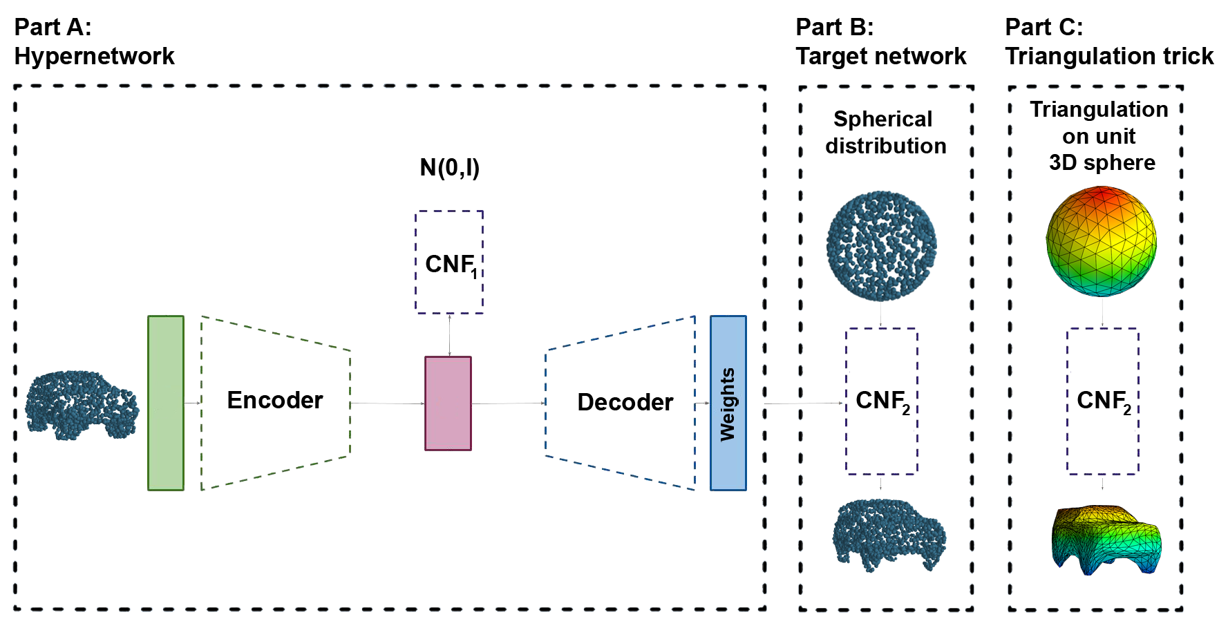
Figure 1: HyperFlow method leverages a hypernetwork architecture to take a 3D point cloud as an input and return parameters of the Continuous Normalizing Flow (CNF) target network (Part A). To represent 3D objects as families of surfaces, we use CNF to parametrize density of point clouds around surfaces with non-compact support distribution called Spherical Log-Normal (Part B). Using this parametrization in the hypernetwork configuration, we can obtain high-quality point cloud reconstructions as well as 3D object meshes (Part C), at a fraction of the training cost required by the vanilla CNF model and with a significantly lower memory footprint.

In this paper, we take a fundamentally different approach to representing 3D objects and, inspired by mesh triangulation methods used in computer graphics [18], we model objects as families of surfaces. More specifically, we consider a point cloud as a sample from a distribution on object surfaces with additive noise introduced by a registration device, such as LIDAR. To model this distribution, we propose a new Spherical Log-Normal function which mimics the topology of 3D objects and provides non-compact support. This, in turn, enables effective utilization of a CNF model as a part of a hypernetwork, instead of a fully-connected neural network as done in HyperCloud [16].

The resulting generative model we introduce in this work, dubbed HyperFlow, produces state-of-the-art generative results both for point clouds and mesh representations. Because we rely on a hypernetwork instead of conditioning a CNF with the autoencoder latent space, our model uses far fewer parameters of the CNF function. As a result, we reduce the training time and corresponding memory footprint of the model by over an order of magnitude with respect to the competing PointFlow.

Our contributions can be summarized as follows:

• We introduce a new HyperFlow generative network that models 3D objects as families of surfaces and allows to build state-of-the-art point cloud representations that can be transformed into 3D meshes by leveraging generative properties of a target network.

• We propose a new Spherical Log-Normal distribution which models a point cloud density with non-compact support and, hence, can be effectively used by a CNF model.

• To the best of our knowledge, our work is the first approach to train a CNF as a target network which reduces its training time and memory footprint by over an order of magnitude, while preserving state-of-the-art generative capabilities.

2 Spherical Log-Normal distribution and the triangulation trick

In this section, we introduce a Spherical Log-Normal distribution that models density of point clouds around surfaces of 3D object and show how it can be used to generate meshes via the so-called triangulation trick.

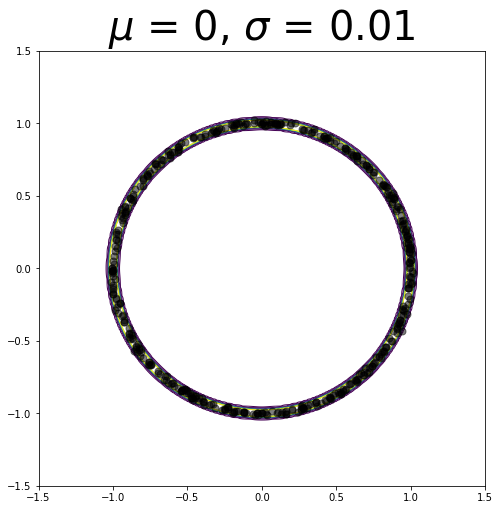
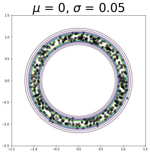
Figure 2: Level sets and samples from Spherical Log-Normal distribution with different parameters $\sigma$ and $\mu=0$. Since Spherical Log-Normal distribution does not have a compact support, it can be used in flow-based architectures.

Since our approach relies on flow-based models, a density distribution has to fulfil several conditions to be used in practice. First of all, flow-based methods cannot be trained on probability distributions with compact support. For instance, it is not possible to train a flow-based model on a 3D ball, as proposed in HyperCloud [16], since computing the log-likelihood cost function used in flows would return infinity for this distribution. As a result, the model does not converge due to numerical instability. Secondly, we would like to model the probability distribution of the surface (mesh representation), which is two-dimensional (the border of a 3D object). Therefore, a Gaussian distribution in $\mathbb{R}^{3}$ is not a good choice, since it models only elements in 3D. Finally, the density distribution should be topologically coherent with the density of the modeled object. More precisely, because of the way registration devices sample space around object surfaces, point clouds are populated with the highest density around object edges and missing points within object structure. Modeling this density with a distribution that does not allow discontinuities is infeasible as per Theorem 2.1 [19].

Theorem 2.1.

There is no continuous invertible map between the 3-ball and the 2-sphere that respects the boundary.

For modeling the surface of an object with a continuous, invertible map, one shall consider the topology of the object [20, 17, 21]. To learn a transformation that is continuous, invertible and provides results close to object boundary, one has to choose a prior that is topologically similar to the expected point cloud, i.e. has the same number of discontinuities. Therefore, we construct a probability distribution on a sphere without compact support.

Spherical Log-Normal distribution on $\mathbb{R}^{n}$.

A probability distribution on a sphere in $\mathbb{R}^{n}$ can by constructed by using one-dimensional density distribution, which takes only positive real values $f:\mathbb{R}_{+}\to\mathbb{R}_{+}.$ In such case, we can define spherical density distribution as:

$$f_{n}:\mathbb{R}^{n}\ni x\to\frac{1}{\mathrm{vol}(S_{n-1})\|x\|^{n-1}}f(\|x\|),$$ (1)

where $\mathrm{vol}(S_{n-1})$ is a surface area of a $n$-dimensional unitary sphere and $f$ is a one-dimensional density, which takes only positive real values. We use one-dimensional density distribution $f:\mathbb{R}_{+}\to\mathbb{R}_{+}$ along radius of unit sphere in all directions. In our model, we use a Log-normal distribution $f(r)=\frac{1}{r}\cdot\frac{1}{\sigma\sqrt{2\pi}}\exp\left(-{\frac{(\log r-\mu)^{2}}{2\sigma^{2}}}\right)$ that is a continuous probability distribution of a random variable, whose logarithm is normally distributed and, hence, provides a non-compact support.

Spherical Log-Normal distribution in $\mathbb{R}^{3}$.

To develop an intuition behind the proposed distribution, we start with a simple visualization in $\mathbb{R}^{2}$. Fig. 2 shows level sets and sample from Spherical Log-Normal distribution with different parameters $\sigma$. Spherical Log-Normal distribution does not have a compact support and can therefore be used in a flow-based architecture. Furthermore, we can force the distribution to concentrate as close as possible to a 2D sphere boundaries.

In $\mathbb{R}^{3}$, our Spherical Log-Normal distribution is defined as:

$$f_{3}(x)=\frac{1}{2(2\pi)^{3/2}\sigma\|x\|^{3}}\exp\left(-\frac{(\log\|x\|-\mu)^{2}}{2\sigma^{2}}\right).$$ (2)

In order to use our distribution in a flow-based model, we need to compute its log-likelihood function:

$$\log f_{3}(x)=-\log(2(2\pi)^{3/2})-\log\sigma-3\log\|x\|-\frac{1}{2\sigma^{2}}(\log\|x\|-\mu)^{2}.$$ (3)

Finally, sampling elements from our Spherical Log-Normal distribution can be done by following a simple procedure. First sample $r$ from one-dimensional Gaussian $N(0,1)$ then sample $x$ from $n$-dimensional Gaussian $N(0,I)$. Sample form Spherical Log-Normal we obtain by the following equation: $\exp(\mu+\sigma\cdot r)\cdot\frac{x}{\|x\|}.$

We avoid numerical instabilities of training by applying a straightforward strategy to find the right values of $\sigma$ parameter: we start with an arbitrary large value of $\sigma$ and reduce it linearly during training.

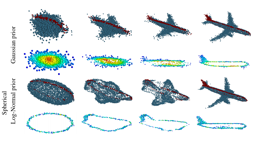
Figure 3: We compare how the prior density is modified for the model with Gaussian prior (upper two rows) and Spherical Log-Normal (bottom two rows). In the first and third row we show how the flow model transforms the original density into the target dataset. The second and fourth row show the cross-sections along the plane depicted by red points. For the Gaussian, target space points are not distributed evenly across the object (a central part of Gaussian distribution is transformed into the bottom of the plane, while its tails are used to model wing tips). For the Spherical Log-Normal, target space points are distributed evenly, across the object, showcasing that our approach truly models the distribution of the points along object surfaces.

Triangulation trick

To model 3D object surfaces as meshes using HyperFlow generative model, we need to investigate the relationship between point clouds and object surfaces. In principle, a point cloud representing a 3D object can be considered a set of samples located on the surface of the object with additive noise introduced by a registration device. We use Spherical Log-Normal to model this distribution with peak density around object surfaces (in 2D, around circle edges, in 3D close to the surface of the sphere) and limited by the radius of the distribution. Once we obtain a parametrized distribution of a point cloud which models object surface together with a registration noise, we can produce a mesh with a simple operation which we call the triangulation trick.

The triangulation trick involves transferring vertices of a sphere mesh through a target network the same way as 3D points, as shown in Part C of Fig 1. Since the target network transforms a sample from a Spherical Log-Normal distribution into a 3D point cloud, when we feed it with a sphere triangulation, it outputs a mesh. In fact, when we substitute samples from Spherical Log-Normal distribution with sphere vertices, we effectively assume minimal registration noise. Processing vertices by the target network pre-trained on point clouds allows us to directly generate denoised mesh representation of object surfaces and obtain a high-quality 3D object rendering. The generative character of our HyperFlow model enables construction of the entire mesh by processing only vertices with a target network, without the need for information about the connections between them, as done in traditional rendering methods.

Fig. 3 presents reconstructions obtained using Gaussian and Spherical Log-Normal distributions. We look at the cross-sections of the reconstructions to observe the main differences on how the input distribution is transformed into a final model by a target network. For the Gaussian distribution, its tails are transformed into object details, such as wing tips and airplane rear aileron. Therefore, we cannot claim that the peak density models surfaces of the object, while its tails model the registration noise. For Spherical Log-Normal, its distribution tails are spread along object surfaces, modeling registration noise. This allows us to produce the final mesh through the triangulation trick, effectively denoising 3D mesh-based object representation and yielding high-quality results, as shown in Fig. 4.

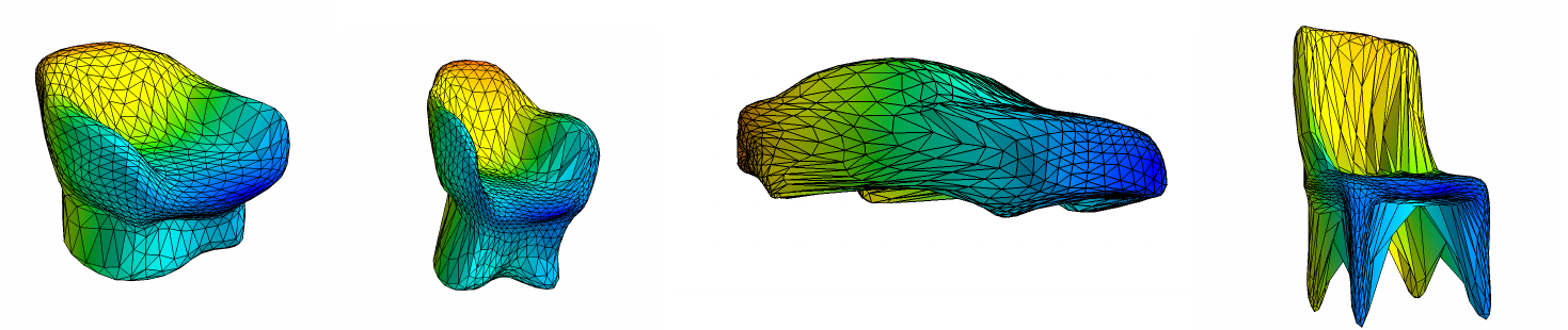
Figure 4: Mesh representations generated by our HyperFlow method. Contrary to the existing methods that return point cloud representations sparsely distributed in 3D space, our approach allows to create a continuous 3D object representation in the form of high-quality meshes.

3 HyperFlow: hypernetwork and Continuous Normalizing Flows for generating 3D point clouds

In this section, we present our HyperFlow model that leverages a hypernetwork framework to train a Continuous Normalizing Flow [17] target network and generate 3D point clouds together with its mesh-based representation. Since HyperFlow encompasses previously introduced autoencoder-based PointFlow [14] with conditioned continuous normalizing flow modules, and HyperCloud method [22], that also leverages hypernetworks, we briefly describe these two approaches before presenting ours.

Autoencoder-based generative model for 3D Point Clouds

Let us first present the autoencoder architecture. The basic aim of autoencoder is to transport the data through a typically, but not necessarily, lower dimensional latent space $\mathcal{Z}=\mathbb{R}^{D}$ while minimizing the reconstruction error. Thus, we search for an encoder $\mathcal{E}:\mathcal{X}\to\mathcal{Z}$ and decoder $\mathcal{D}:\mathcal{Z}\to\mathcal{X}$ functions, which minimizes the reconstruction error. In the Autoencoder-based generative model we additionally ensure that the data transported to the latent comes from the prior distribution (typically Gaussian one) [23, 24, 25].

Continuous normalizing flow

Generative models are one of the fastest growing areas of deep learning. Variational Autoencoders (VAE) [23] and Generative Adversarial Networks (GAN) [26] are the most popular approaches. Another model gained popularity – Normalizing Flow (NF) [20]. A flow-based generative model is constructed by a sequence of invertible transformations. Unlike the other two methods mentioned previously, the model explicitly learns the data distribution and therefore the loss function is simply the negative log-likelihood.

Normalizing Flow (NF) [20] is able to model complex probability distributions. A normalizing flow transforms a simple prior distribution (usually Gaussian one) $\mathcal{P}(Y)$ into a complex one (represented by data distribution $X$) by applying a sequence of invertible transformation functions: $f_{1},\ldots,f_{n}:Y\to X$. Flowing through a chain of transformations $x=F(y)=f_{n}\circ f_{n-1}\circ\ldots\circ f_{1}(y),$ we obtain a probability distribution of the final target variable.

Then the probability density of the output variable is given by the change of variables formula:

$$\log P(x)=\log P(y)-\sum_{k=1}^{n}\log\left|\det\frac{\partial f_{k}}{\partial y_{k-1}}\right|,$$ (4)

where $y$ can be computed from $x$ using the inverse flow: $y=f^{-1}_{1}\circ f^{-1}_{2}\circ\ldots\circ f^{-1}_{n}(x).$ In such framework, both the inverse map and the determinant of the Jacobian should be computable.

The continuous normalizing flow [27] is a modification of the above approach, where instead of a discrete sequence of iterations we allow the transformation to be defined by a solution to a differential equation $\frac{\partial y(t)}{\partial t}=f(y(t),t),$ where $f$ is a neural network that has an unrestricted architecture. Continuous Normalizing Flows (CNF ) $F_{\theta}:Y\ni y\to x\in X$ is a solution of differential equations with the initial value problem $y(t_{0})=x$, $\frac{\partial y(t)}{\partial t}=f_{\theta}(y(t),t)$. In such a case we have

$$F(y)=F_{\theta}(y(t_{0}))=y(t_{0})+\int^{t_{1}}_{t_{0}}f_{\theta}(y(t),t)dt,\mbox{ and }F_{\theta}^{-1}(x)=x+\int_{t_{1}}^{t_{0}}f_{\theta}(y(t),t)dt,$$ (5)

where $f_{\theta}$ defines the continuous-time dynamics of the flow $F_{\theta}$ and $y(t_{1})=x$.

The log probability cost function with prior distribution with density $g$ can be computed by:

$$\mathcal{C}_{F}(X;g,\theta)=\sum_{x\in X}\log g(F_{\theta}^{-1}(x))-\int^{t_{1}}_{t_{0}}\mathrm{Tr}\left(\frac{\partial f_{\theta}}{\partial y(t)}\right)dt.$$ (6)

In PointFlow [14] authors show that CNF can be used for modeling 3D objects. Instead of directly parametrizing the distribution of points in a shape (fixed size 3D point cloud), PointFlow models this distribution as an invertible parameterized transformation of 3D points from a prior distribution (e.g., a 3D Gaussian). Intuitively, under this model, generating points for a given shape involves sampling points from a generic Gaussian prior, and then moving them according to this parameterized transformation to their new location in the target shape.

Hypernetwork

Hypernetworks, introduced in [22], are defined as neural models that generate weights for a separate target network solving a specific task. Making an analogy between hypernetworks and generative models, the authors of [28], use this mechanism to generate a diverse set of target networks approximating the same function. Hypernetworks can also be used for functional representations of images [29].

In the case of generating 3D point clouds, objects are represented by a neural network. Autoencoder based architecture "produces" the neural network which transforms prior distribution into elements from a point cloud. In HyperCloud [16] autoencoder based architecture takes as an input point cloud and directly produces weights to another neural network, which models elements from a 3D object.

HyperFlow

In this section, we present details of our novel model dubbed HyperFlow which encompasses and extends prior works by training continuous normalizing flow modules to model 3D point cloud distributions with a hypernetwork framework. Our model is inspired by a Variational Autoencoder (VAE) [23, 30] framework that allows learning $\mathcal{P}(X)$ from a dataset of observations of $X$. VAE models data distribution via a latent variable $z$ with a prior distribution $\mathcal{P}_{\psi}(z)$, and a decoder $\mathcal{P}_{\theta}(X|z)$ which reconstructs the distribution of $X$ condition on a given $z$. The model is trained together with an encoder $\mathcal{Q}_{\phi}(z|X)$ by minimizing the lower bound on the log-likelihood of the observations (ELBO).

Instead of using a Gaussian prior over shape representations as done in [14], we add another CNF to model a learnable prior $\mathcal{P}_{\psi}$. The corresponding ELBO cost function can be rewritten after [14] as:

$$\mathcal{L}(X;\phi,\psi,\theta)=\underbrace{\mathbb{E}_{\mathcal{Q}_{\phi}(z|X)}\left[\log\mathcal{P}_{\theta}(X|z)\right]}_{\text{Reconstruction}}+\underbrace{\mathbb{E}_{\mathcal{Q}_{\phi}(z|X)}\left[\log\mathcal{P}_{\psi}(z)\right]+H\left[\mathcal{Q}_{\phi}(z|X)\right]}_{\text{Latent representation}},$$ (7)

where $H$ is the entropy and $\mathcal{P}_{\psi}(z)$ is the prior distribution with trainable parameters $\psi$.

We propose to adapt the above cost function to a hypernetwork framework. We therefore introduce our HyperFlow model that consists of two main parts, as shown in Fig. 1. The first one is a hypernetwork that outputs weights (Fig. 1 Part A) of another neural network. The second one is a target network (Fig. 1 Part B) which models the distribution of elements on the surface of a 3D object. Using autoencoder terminology, we define three elements: an encoder, a decoder and a prior distribution.The encoder $\mathcal{E}_{\phi}:\mathcal{X}\to\mathcal{Z}$ can reduce data dimensionality by mapping it to a lower-dimensional latent space $\mathcal{Z}\subseteq\mathbb{R}^{D}$. We follow [31] and use a simple permutation-invariant encoder to predict $\mathcal{E}_{\phi}$.

We use $\mathcal{P}_{\mathcal{Z}}$ over shape representations proposed by PointFlow [14]. The assumed probability distribution on the latent pace can be more complex than the commonly used $N(0,I)$ and not given in an explicit form. In such a framework, we use an additional continuous normalizing flow $G_{\psi}$, which transfers latent space into a Gaussian prior. Finally, we propose to use a decoder that returns weights of the target network $\mathcal{D}_{\theta}:\mathcal{Z}\ni z\to\Theta$, instead of 3D points as done in [14, 15]. The resulting hypernetwork contains an encoder $\mathcal{E}_{\phi}$, a decoder $\mathcal{D}_{\theta}$ and a flow $G_{\psi}$ (Fig. 1 Part A).

The hypernetwork takes as an input a point-cloud $X\subset\mathbb{R}^{3}$ and returns weights $\Theta$ to $f_{\Theta}$ that defines the continuous-time dynamics of the flow $F_{\Theta}$. CNF takes an element from the prior distribution $\mathcal{P}$ and transfers it to an element on the surface of the object, see Part B: target network in Fig. 1. In our work, we use a Free-form Jacobian of Reversible Dynamics (FFJORD) [17] and transformation between Spherical Log-Normal distribution and the 3D object. As presented in Sec. 2 this choice of distribution function allows one to create a continuous mesh representation with the triangulation trick.

The cost function of HyperFlow consists of two parts. The first one correspond to hypernetwork. This part of the architecture is similar to PointFlow. The second one is a cost function of CNF corresponding to target network. The final cost function of our HyperFlow model can be calculated using Eq. (7):

$$\mathcal{C}_{H}(X;\theta,\phi,\psi)=\underbrace{\mathcal{C}_{F}(X;f_{3},\Theta_{\theta,\phi,\psi})}_{\text{ Target network cost function }}+\underbrace{\mathcal{C}_{G}(\mathcal{E}_{\phi}(X);N(0,1),\psi)+H(\mathcal{E}_{\phi}(X))}_{\text{ Hypernetwork cost function }},$$

where $H$ is the entropy function, $\mathcal{C}_{F}$ is a CNF cost function between point cloud $X$ and Spherical Log-Normal density $f_{3}$ and $\mathcal{C}_{G}$ is a CNF cost function between latent representation $\mathcal{E}_{\phi}(X)$ and a Gaussian prior.

	Airplane					Chair					Car
Method	JSD	MMD		COV		JSD	MMD		COV		JSD	MMD		COV
		CD	EMD	CD	EMD		CD	EMD	CD	EMD		CD	EMD	CD	EMD
l-GAN	3.61	0.269	3.29	47.90	50.62	2.27	2.61	7.85	40.79	41.69	2.21	1.48	5.43	39.20	39.77
PC-GAN	4.63	0.287	3.57	36.46	40.94	3.90	2.75	8.20	36.50	38.98	5.85	1.12	5.83	23.56	30.29
PointFlow	4.92	0.217	3.24	46.91	48.40	1.74	2.42	7.87	46.83	46.98	0.87	0.91	5.22	44.03	46.59
HyperCloud	4.84	0.266	3.28	39.75	43.70	2.73	2.56	7.84	41.54	46.67	3.09	1.07	5.38	40.05	40.05
HyperFlow	5.39	0.226	3.16	46.66	51.60	1.50	2.30	8.01	44.71	46.37	1.07	1.14	5.30	45.74	47.44

Table 1: Generation results. MMD-CD scores are multiplied by $10^{3}$; MMD-EMD scores and JSDs are multiplied by $10^{2}$.

4 Experiments

In this section, we present the evaluation of our model against the competing methods on two tasks: 3D point clouds generation and 3D mesh generation. Furthermore, we test the efficiency of our approach in terms of training time and memory footprint. All experiments are done on a stationary unit with a Nvidia GeForce GTX 1080 GPU. If not stated otherwise, default parameters are used.

Generating 3D point clouds

We compare the generative capabilities with competing approaches: latent-GAN [31], PC-GAN [32], PointFlow [14], HyperCloud [16]. We follow the evaluation protocol of [14] and train each model using point clouds from one of the three categories in the ShapeNet dataset [33]: airplane, chair, and car. Tab. 1 presents the results and shows that HyperFlow obtains comparable or superior generative results to the state-of-the-art PointFlow method.

Generating 3D meshes

The main advantage of our method, when compare to the reference solutions, is the ability to generate high-quality 3D point clouds as well as meshes using the triangulation trick presented in Sec. 2. For evaluation of the quality of mesh grid representation, we follow the evaluation protocol of [16]. For PointFlow, we use the triangulation trick and create object meshes by feeding the target network a 3D sphere. For HyperCloud and our HyperFlow method we use a sphere with radius $R=1$. As can be seen in Tab. 2, PointFlow that uses a Gaussian distribution as a prior provides results inferior to HyperCloud and HyperFlow, while our HyperFlow method offers the best performance, thanks to using Spherical Log-Normal as a prior instead of a compact support distribution function as in HyperCloud. More qualitative mesh results as well as detailed description of metrics used in our experiments can be found in the supplementary material.

Training time and memory footprint comparison

	Airplane					Chair					Car
Sphere R	JSD	MMD		COV		JSD	MMD		COV		JSD	MMD		COV
		CD	EMD	CD	EMD		CD	EMD	CD	EMD		CD	EMD	CD	EMD
PointFlow
R=2.795	22.26	0.49	6.65	44.69	20.74	19.28	4.28	13.38	36.85	20.84	16.59	1.6	8.00	20.17	17.04
R=3.136	26.46	0.60	6.89	39.50	19.01	22.52	4.89	14.47	32.47	17.22	20.21	1.75	7.80	21.59	17.3
R=3.368	29.65	0.68	6.84	40.49	16.79	24.68	5.36	14.97	31.41	17.06	24.10	1.96	8.35	18.75	17.04
HyperCloud
R=1	9.51	0.45	5.29	30.60	28.88	4.32	2.81	9.32	40.33	40.63	5.20	1.11	6.54	37.21	28.40
HyperFlow
R=1	6.55	0.38	3.65	40.49	48.64	4.26	3.33	8.27	41.99	45.32	5.77	1.39	5.91	28.40	37.21

Table 2: The values of quality measures of 3D representations obtained by sampling from sphere of a given radius $R$ for airplane, chair and car shapes. HyperFlow generates higher quality of point cloud representation than those of PointFlow and HyperCloud.

Fig. 5 displays a comparison between our HyperFlow method and the competing PointFlow. For a fair comparison we evaluated the architectures used in the previous sections that obtain best quantitative results. The models were trained on the car dataset. Our HyperFlow approach leads to a significant reduction in both training time and memory footprint due to a more compact flow architecture enabled by a hypernetwork framework.

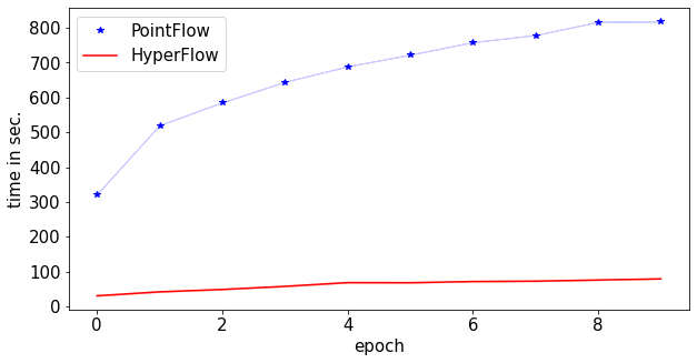
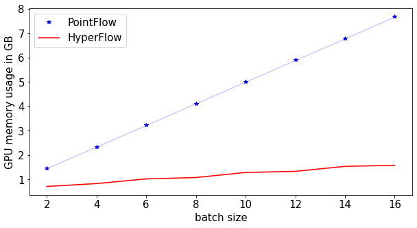
Figure 5: Comparison of training times and GPU memory used by PointFlow and HyperFlow. Our HyperFlow method offers over an order of magnitude decrease in both training time and memory.

5 Conclusions

In this work, we introduce a novel HyperFlow method that uses a hypernetwork to model 3D objects as families of surfaces and, hence, allows to build state-of-the-art point cloud reconstructions and mesh-based object representations. To model a distribution of a point cloud we propose a new Spherical Log-Normal distribution with non-compact support that can be effectively used by a CNF model. Finally, we believe our work is the first approach to train CNF as a target network which reduces training cost and opens new research paths for modeling complex 3D structures, such as indoor scenes.

Broader Impact

This research can be beneficial for researchers and engineers working in the space of 3D point clouds and related registration devices, such as LIDARs and depth cameras. As such, the proposed methods can be used in the context of autonomous driving and robotics. Further extensions of this work can be beneficial for people with disparities, especially related to sensory disorders, such as shortsightedness or blindness, as 3D capturing devices can effectively extend their way of interacting and perceiving the external world. On the other hand, robotic automation resulting from this work can potentially put at disadvantage people whose livelihoods depend on manual execution of jobs that can be substituted with robotics. In case of system failure, the consequences include problems with handling outputs of registration devices, such as LIDARs and depth cameras. Our method does not leverage any biases in the data.

6 Supplementary material

In this supplementary material, we first present the full description of evaluation metrics used in the experiments. We then describe two experiments showing the relationship between Gaussian distribution and Spherical Log-Normal distribution proposed in our work. Finally, we show an extended set of visualizations obtained by HyperFlow.

6.1 Description of evaluation metrics

Following the methodology for evaluating generative fidelity and diversification among samples proposed in [31] and [14], we use the following evaluation metrics: Jensen-Shannon Divergence, Coverage, Minimum Matching Distance 1-nearest Neighbor Accuracy.

Jensen-Shannon Divergence (JSD): a measure of the distance between two empirical distributions $P$ and $Q$, defined as:

$$\begin{array}[]{c}JSD(P\|Q)\!=\!\frac{KL(P\|M)+KL(Q\|M)}{2},\mbox{ where }M\!=\!\frac{P+Q}{2}.\end{array}$$

Coverage (COV): a measure of generative capabilities in terms of richness of generated samples from the model. For two point cloud sets $X_{1},X_{2}\subset\mathbb{R}$ coverage is defined as a fraction of points in $X_{2}$ that are in the given metric the nearest neighbor to some points in $X_{1}$.

Minimum Matching Distance (MMD): since COV only takes the closest point clouds into account and does not depend on the distance between the matchings additional metric was introduced. For point cloud sets $X_{1}$, $X_{2}$ MMD is a measure of similarity between point clouds in $X_{1}$ to those in $X_{2}$.

We examine the generative capabilities of our HyperFlow model with respect to the existing reference approaches. We strictly follow the methodology presented in [14]. We train each model using point clouds from one of the three categories in the ShapeNet dataset: airplane, chair, and car.

6.2 Scheduling parameters of Spherical Log-Normal

In our model we use Spherical Log-Normal density with $m=0$ and $\sigma=0.001$. Using Spherical Log-Normal density with small $\sigma=0.001$ might be unstable since density distributing has small tails, see Fig. 2 (in main paper). At the beginning of training a log-likelihood cost function in some points might be close to zeros (numerically unstable).

Therefore, in the training procedure we start with large $\sigma=1$ and reduce such parameter to $\sigma=0.001$. We use linear scheduling. In the case of starting $\sigma_{0}$ and final value of $\sigma_{1}$ with $n$ epochs we reduce the parameter by $\Delta\sigma=\frac{\sigma_{1}-\sigma_{0}}{n}$ in each epoch.

Our model is approximately 10 times faster than PointFlow (see experimental section in main paper), and can be easily trained on HyperFlow density. In PointFlow architecture is larger and it is diffitult to train such model on our distribution from scratch. This process can be accelerated by using pre-trained model on classical Gaussian distribution. In such a case we can start from Spherical Log-Normal distribution with parameters $\mu$ and $\sigma$ which approximate Gaussian distribution (see Theorem 6.1). In Fig. 6 we present comparison between samples from Gaussian distribution and Spherical Log-Normal distribution with such parameters. Thanks to such solution we can take a model already trained on Gaussian distribution and train it further with our strategy.

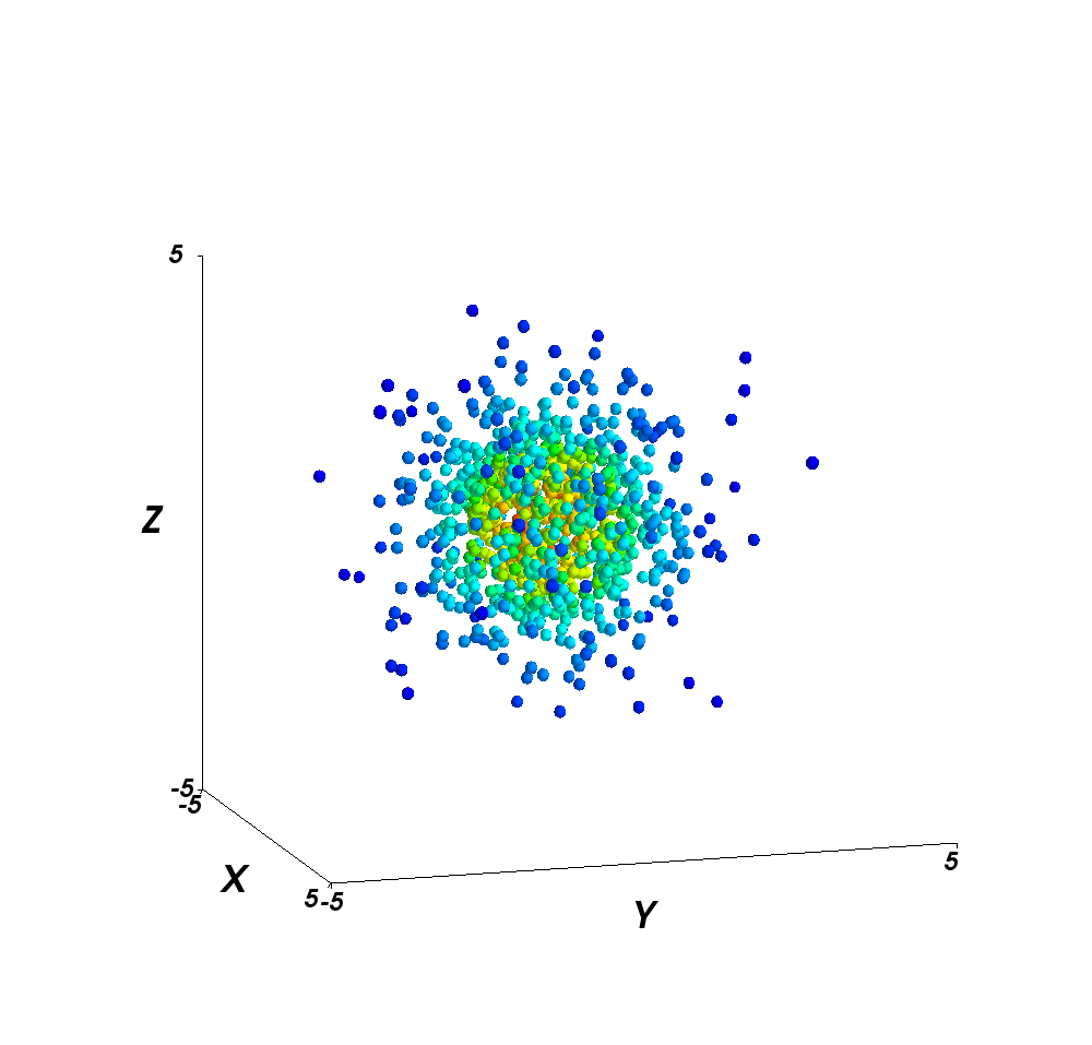
Figure 6: Comparison between samples from a Gaussian distribution (left) and Spherical Log-Normal distribution (right) which approximates normal distribution (with parameters from Theorem 6.1).

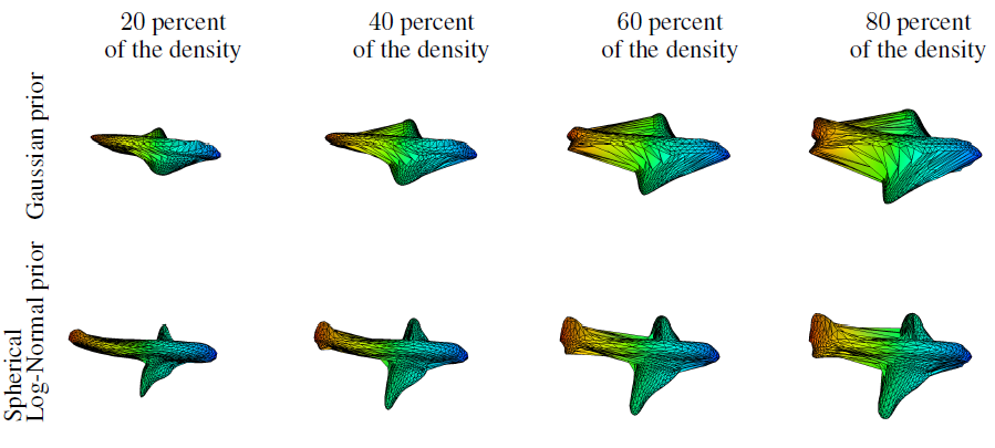
Figure 7: Object meshes generated for different radii. For the Gaussian prior, the quality and size of the mesh heavily depends on the radius size, while for Spherical Log-Normal the quality and size remains stable across radii sizes.

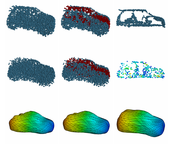
Figure 8: In the first row, we present a car from a data-set which contains elements inside objects. In the second row, we present reconstructions of the object. In the third row, we show meshes generated by radii which contains $40,60$ and $80$ percent of the density. As we can see, radius containing $80$ percent of the density generate the best mesh.

Theorem 6.1.

Classical Gaussian distribution in $\mathbb{R}^{3}$ can be approximated by Spherical Log-Normal distribution (with log normal distribution) with parameters:

$$\mu=\log(8/\pi)-\frac{1}{2}\log(3)\mbox{ and }\sigma=\log(3\pi/8).$$

Proof.

Observe that both Gaussian and Spherical Log-Normal distributions are spherical. This means that to compare them it is enough to consider the distributions of the radius. In the case of Gaussian in $\mathbb{R}^{3}$, the distribution of radius is given by $\chi_{3}$ distribution, which has mean and variance given by

$$\begin{array}[]{rcl}\mu_{\chi_{3}}&=&\sqrt{2}\cdot\Gamma[(3+1)/2]/\Gamma[3/2]=2\sqrt{2/\pi},\\[4.30554pt] \sigma^{2}_{\chi_{3}}&=&3-(\mu_{\chi_{3}})^{2}=3-\frac{8}{\pi}.\end{array}$$

On the other hand, Log-Normal (LN) distribution with parameters $m$ and $\sigma$ has mean and variance given by

$$\begin{array}[]{rcl}\mu_{LN}&=&\exp(\mu+\sigma^{2}/2),\\[4.30554pt] \sigma^{2}_{LN}&=&(\exp(\sigma^{2})-1)\exp(2(\mu+\sigma^{2}/2)).\end{array}$$

Now we have to solve above system of equations and calculate parameters $\mu,\sigma$ by $\mu_{\chi_{3}}$ i $\sigma_{\chi_{3}}$.

∎

6.3 Families of surfaces

In this section we would like to describe in a more detailed way, how HyperFlow approximates objects by families of surfaces. Let us recall that Fig. 3 of the main paper compares how the prior density is modified for the model with Gaussian prior and Spherical Log-Normal. For the Gaussian distribution, its tails are transformed into object details, such as wing tips and airplane rear aileron. Therefore, we cannot claim that the peak density models surfaces of the object, while its tails model the registration noise, as is the case for our Spherical Log-Normal distribution. For Spherical Log-Normal, the distribution tails are spread along object surfaces, modeling registration noise. This allows us to produce the final mesh through the triangulation trick, effectively denoising 3D mesh-based object representation and yielding high-quality results. In HyperFlow we use triangulation on unit sphere. It is motivated by the fact that point on surfaces has symmetric noise (gaussian noise). Nevertheless, we can use triangulation on sphere with different radii (corresponding to different percent of the density). To compare the models, for both of them we can draw the images of spheres which contain inside the same percentage of the data. In such a case we obtain families of surfaces. In Fig. 7 we present meshes obtained by different radii which contains $20,40,60$ and $80$ percent of the density. Spherical Log-Normal stabilizes triangulation, while for model with normal prior relatively high fluctuations can be observed.

Usually, it is enough to use triangulation on unit sphere. But in some cases we can obtain better meshes by changing radius of the sphere. For instance, some elements from ShapeNet do not contain only surfaces of objects. In the case of some cars, we have additional elements like steering wheel, see Fig. 8. In such a case, we can use triangulation trick with a larger radius sphere for obtaining better mesh representation, see Fig. 8.

6.4 Visualization of mesh representation obtained by HyperFlow

Below we present:

• Fig. 9: Mesh representations generated by our HyperFlow method - extended version of the meshes presented in the main paper.

• Fig. 10 and Fig. 11: Visualizations of how the triangulation on the sphere is transformed into a mesh of an object.

• Fig 12: Visualizations on how the samples from our Spherical Log-Normal prior are transformed into points on objects.

Overall, our HyperFlow method offers stable and high-quality object meshes at significantly lower computation cost than the competing point cloud generative models.

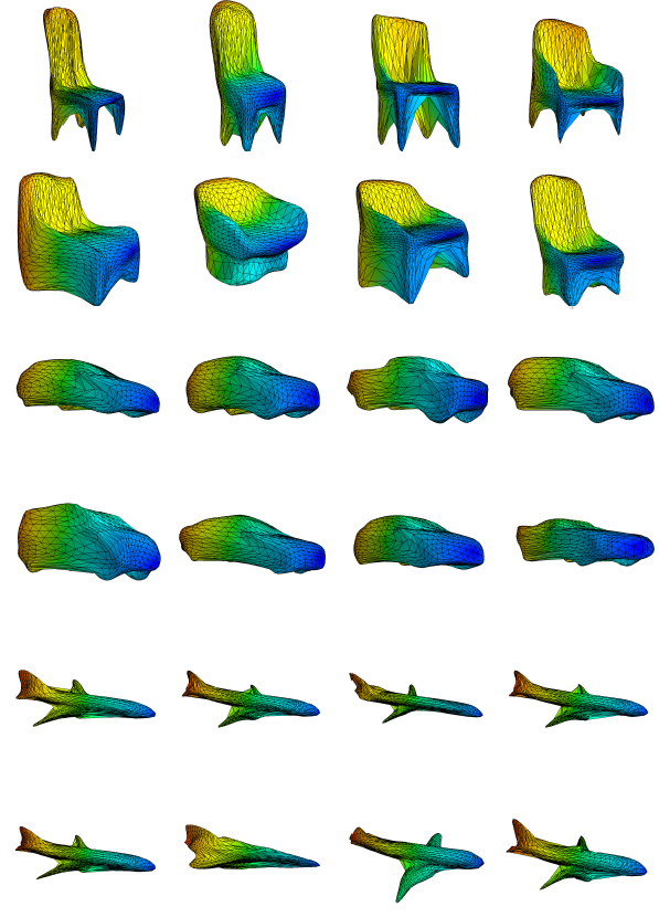
Figure 9: Mesh representations generated by our HyperFlow method. Contrary to the existing methods that return point cloud representations sparsely distributed in 3D space, our approach allows to create a continuous 3D object representation in the form of high-quality meshes.

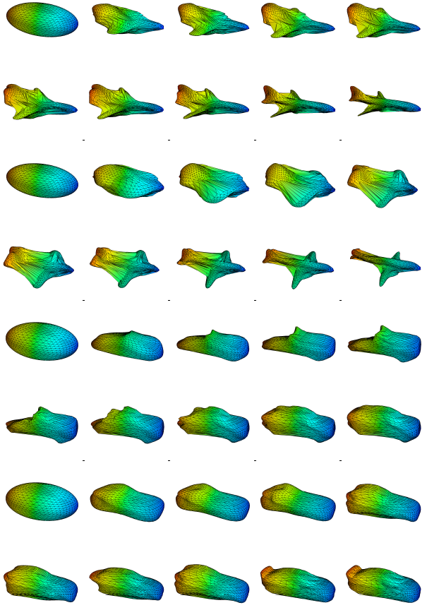
Figure 10: In the image we present how the triangulation on the sphere is transformed into mesh of object. As we can see, thanks to triangulation trick we obtain high quality mesh. Thanks to us CNF as a target network we can visualize continuous transformation between uniform sphere and surfaces of objects.

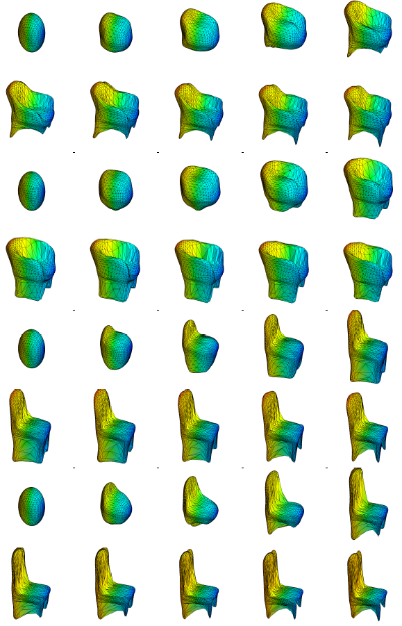
Figure 11: We show how the triangulation on the sphere is transformed into a mesh of object. Thanks to the so-called triangulation trick, we obtain high quality object meshes. Since we use a CNF as a target network, we can visualize a continuous transformation between a uniform sphere and surfaces of objects.

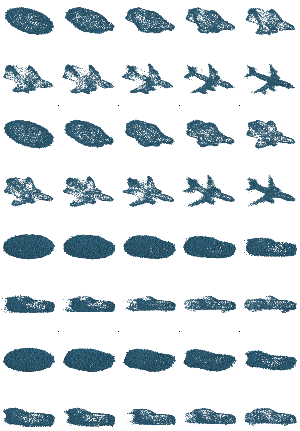
Figure 12: We visualize how the samples from prior (Spherical Log-Normal) are transformed into points on object surfaces. The transformation produces a point representation of a similar quality to PiontFlow.

References

- [1] Ben Kehoe, Sachin Patil, Pieter Abbeel, and Ken Goldberg. A survey of research on cloud robotics and automation. IEEE Transactions on automation science and engineering, 12(2):398–409, 2015.
- [2] Bin Yang, Wenjie Luo, and Raquel Urtasun. Pixor: Real-time 3d object detection from point clouds. In Proceedings of the IEEE conference on Computer Vision and Pattern Recognition, pages 7652–7660, 2018.
- [3] Jeong Joon Park, Peter Florence, Julian Straub, Richard Newcombe, and Steven Lovegrove. Deepsdf: Learning continuous signed distance functions for shape representation. In Proceedings of the IEEE Conference on Computer Vision and Pattern Recognition, pages 165–174, 2019.
- [4] Wang Yifan, Shihao Wu, Hui Huang, Daniel Cohen-Or, and Olga Sorkine-Hornung. Patch-based progressive 3d point set upsampling. In Proceedings of the IEEE Conference on Computer Vision and Pattern Recognition, pages 5958–5967, 2019.
- [5] Lequan Yu, Xianzhi Li, Chi-Wing Fu, Daniel Cohen-Or, and Pheng-Ann Heng. Pu-net: Point cloud upsampling network. In Proceedings of the IEEE Conference on Computer Vision and Pattern Recognition, pages 2790–2799, 2018.
- [6] Zhirong Wu, Shuran Song, Aditya Khosla, Fisher Yu, Linguang Zhang, Xiaoou Tang, and Jianxiong Xiao. 3d shapenets: A deep representation for volumetric shapes. In Proceedings of the IEEE conference on computer vision and pattern recognition, pages 1912–1920, 2015.
- [7] Jiajun Wu, Chengkai Zhang, Tianfan Xue, Bill Freeman, and Josh Tenenbaum. Learning a probabilistic latent space of object shapes via 3d generative-adversarial modeling. In Advances in neural information processing systems, pages 82–90, 2016.
- [8] Hang Su, Subhransu Maji, Evangelos Kalogerakis, and Erik Learned-Miller. Multi-view convolutional neural networks for 3d shape recognition. In Proceedings of the IEEE international conference on computer vision, pages 945–953, 2015.
- [9] Shuiwang Ji, Wei Xu, Ming Yang, and Kai Yu. 3d convolutional neural networks for human action recognition. IEEE transactions on pattern analysis and machine intelligence, 35(1):221–231, 2012.
- [10] Daniel Maturana and Sebastian Scherer. Voxnet: A 3d convolutional neural network for real-time object recognition. In 2015 IEEE/RSJ International Conference on Intelligent Robots and Systems (IROS), pages 922–928. IEEE, 2015.
- [11] Manzil Zaheer, Satwik Kottur, Siamak Ravanbakhsh, Barnabas Poczos, Russ R Salakhutdinov, and Alexander J Smola. Deep sets. In Advances in neural information processing systems, pages 3391–3401, 2017.
- [12] Charles R Qi, Hao Su, Kaichun Mo, and Leonidas J Guibas. Pointnet: Deep learning on point sets for 3d classification and segmentation. In Proceedings of the IEEE Conference on Computer Vision and Pattern Recognition, pages 652–660, 2017.
- [13] Charles Ruizhongtai Qi, Li Yi, Hao Su, and Leonidas J Guibas. Pointnet++: Deep hierarchical feature learning on point sets in a metric space. In Advances in neural information processing systems, pages 5099–5108, 2017.
- [14] Guandao Yang, Xun Huang, Zekun Hao, Ming-Yu Liu, Serge Belongie, and Bharath Hariharan. Pointflow: 3d point cloud generation with continuous normalizing flows. In Proceedings of the IEEE International Conference on Computer Vision, pages 4541–4550, 2019.
- [15] Michał Stypułkowski, Maciej Zamorski, Maciej Zięba, and Jan Chorowski. Conditional invertible flow for point cloud generation. arXiv preprint arXiv:1910.07344, 2019.
- [16] Przemysław Spurek, Sebastian Winczowski, Jacek Tabor, Maciej Zamorski, Maciej Zięba, and Tomasz Trzciński. Hypernetwork approach to generating point clouds. Proceedings of the 37th International Conference on Machine Learning (ICML), 2020.
- [17] Will Grathwohl, Ricky TQ Chen, Jesse Betterncourt, Ilya Sutskever, and David Duvenaud. Ffjord: Free-form continuous dynamics for scalable reversible generative models. arXiv preprint arXiv:1810.01367, 2018.
- [18] Herbert Edelsbrunner. Triangulations and meshes in computational geometry. Acta Numerica, 9:133–213, 2000.
- [19] Austin Dill, Chun-Liang Li, Songwei Ge, and Eunsu Kang. Getting topology and point cloud generation to mesh. CoRR, abs/1912.03787, 2019.
- [20] Danilo Jimenez Rezende and Shakir Mohamed. Variational inference with normalizing flows. arXiv preprint arXiv:1505.05770, 2015.
- [21] Jens Behrmann, Will Grathwohl, Ricky TQ Chen, David Duvenaud, and Jörn-Henrik Jacobsen. Invertible residual networks. arXiv preprint arXiv:1811.00995, 2018.
- [22] David Ha, Andrew Dai, and Quoc V Le. Hypernetworks. arXiv preprint arXiv:1609.09106, 2016.
- [23] Diederik P Kingma and Max Welling. Auto-encoding variational bayes. arXiv preprint arXiv:1312.6114, 2013.
- [24] Ilya Tolstikhin, Olivier Bousquet, Sylvain Gelly, and Bernhard Schoelkopf. Wasserstein auto-encoders. arXiv preprint arXiv:1711.01558, 2017.
- [25] Jacek Tabor, Szymon Knop, Przemysław Spurek, Igor Podolak, Marcin Mazur, and Stanisław Jastrzębski. Cramer-wold autoencoder. arXiv preprint arXiv:1805.09235, 2018.
- [26] Ian Goodfellow, Jean Pouget-Abadie, Mehdi Mirza, Bing Xu, David Warde-Farley, Sherjil Ozair, Aaron Courville, and Yoshua Bengio. Generative adversarial nets. In Advances in neural information processing systems, pages 2672–2680, 2014.
- [27] Tian Qi Chen, Yulia Rubanova, Jesse Bettencourt, and David K Duvenaud. Neural ordinary differential equations. In Advances in neural information processing systems, pages 6571–6583, 2018.
- [28] Abdul-Saboor Sheikh, Kashif Rasul, Andreas Merentitis, and Urs Bergmann. Stochastic maximum likelihood optimization via hypernetworks. arXiv preprint arXiv:1712.01141, 2017.
- [29] Sylwester Klocek, Lukasz Maziarka, Maciej Wolczyk, Jacek Tabor, Jakub Nowak, and Marek Smieja. Hypernetwork functional image representation. In International Conference on Artificial Neural Networks, pages 496–510. Springer, 2019.
- [30] Danilo Jimenez Rezende, Shakir Mohamed, and Daan Wierstra. Stochastic backpropagation and approximate inference in deep generative models. arXiv preprint arXiv:1401.4082, 2014.
- [31] Panos Achlioptas, Olga Diamanti, Ioannis Mitliagkas, and Leonidas Guibas. Learning representations and generative models for 3d point clouds. arXiv preprint arXiv:1707.02392, 2017.
- [32] Chun-Liang Li, Manzil Zaheer, Yang Zhang, Barnabas Poczos, and Ruslan Salakhutdinov. Point cloud gan. arXiv preprint arXiv:1810.05795, 2018.
- [33] Angel X. Chang, Thomas A. Funkhouser, Leonidas J. Guibas, Pat Hanrahan, Qi-Xing Huang, Zimo Li, Silvio Savarese, Manolis Savva, Shuran Song, Hao Su, Jianxiong Xiao, Li Yi, and Fisher Yu. Shapenet: An information-rich 3d model repository. CoRR, abs/1512.03012, 2015.