Abstract

We show that molecular dynamics (MD) simulations are capable of reproducing the drag of solute segregation atmospheres by moving grain boundaries (GBs). Although lattice diffusion is frozen out on the MD timescale, the accelerated GB diffusion provides enough atomic mobility to allow the segregated atoms to follow the moving GB. This finding opens the possibility of studying the solute drag effect with atomic precision using the MD approach. We demonstrate that a moving GB activates diffusion and alters the short-range order in the lattice regions swept during its motion. It is also shown that a moving GB drags an atmosphere of non-equilibrium vacancies, which accelerate diffusion in surrounding lattice regions.

I Introduction

Grain boundaries (GBs) are critical components of microstructure that often control properties and performance of materials (Sutton and Balluffi, 1995; Mishin et al., 2010). In alloys, GBs can interact with the chemical components by a number of different mechanisms. A stationary GB can form a segregation atmosphere that reduces its free energy and alters its mechanical responses, thermal, electronic, and other properties. When a GB moves under an applied thermodynamic driving force, its interaction with the alloy components can drastically change its mobility.

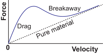
Figure 1: Schematic force-velocity diagram according to the classical model of GB solute drag (Cahn, 1962; Lücke and Stüwe, 1963, 1971). The maximum of the force separates two kinetic regimes. The moving GB drags the segregation atmosphere at low velocities and breaks away from it at high velocities.

One of the interaction mechanisms is the drag of the segregation atmosphere by a moving GB. The effect is known as the GB solute drag and has been the subject of numerous experimental, theoretical and modeling studies over the past decades. The first quantitative model of solute drag was proposed by Cahn (Cahn, 1962) and LÃŒcke et al. (Lücke and Stüwe, 1963, 1971). Their model predicts a highly nonlinear relation between the GB velocity and the drag (friction) force, with a maximum force reached at some critical velocity (Fig. 1). On the low-velocity side of the maximum, the segregation atmosphere moves together with the GB. Dragging the entire atmosphere requires a larger driving force than for moving the same GB through a uniform solution. On the high-velocity side of the maximum, the GB breaks away from the atmosphere and the drag force drops. Eventually, the GB forms a new, much lighter segregation atmosphere that poses less resistance to its motion.

The solute drag effect has been studied by a number of simulation approaches, including the phase field (Ma et al., 2003; Li et al., 2009; Shahandeh et al., 2012; Grönhagen and Agren, 2007; Abdeljawad et al., 2017) and phase-field crystal (Greenwood et al., 2012) methods, atomic-level computer simulations (Mendelev and Srolovitz, 2002; Sun and Deng, 2014; Wicaksono et al., 2013; Mendelev et al., 2001; Rahman et al., 2016; Kim and Park, 2008), and discrete quasi-1D models (Ma et al., 2003; Mishin, 2019). Another effective approach to studying the solute drag is offered by molecular dynamics (MD) simulations. MD provides access to all atomic-level details of the GB motion and permits continual tracking of both the GB velocity and the driving force. No approximations are made other than the atomic interaction model (interatomic potential), which for some systems can be quantitatively accurate. Unfortunately, the timescale of MD simulations is presently limited to tens, or at best a hundred, nanoseconds. This timescale is too short to capture lattice diffusion by the vacancy mechanism. Given the small concentration of equilibrium vacancies and the low vacancy-atom exchange rate, an average atom can only make a few jumps in a typical MD simulation. Meanwhile, the classical solute drag model (Cahn, 1962; Lücke and Stüwe, 1963, 1971) assumes that the solute atoms diffuse toward or away from the moving GB through the lattice at a finite rate. Accordingly, the lattice diffusion coefficient is one of the parameters of the model.

Because of the timescale disparity mentioned above, a common perception has been that the MD method is not suitable for direct simulations of the solute drag. More precisely, in MD simulations, it is always possible to drag a GB through a solid solution. This will generally require a larger driving force than in a single-component system. As such, the simulations will capture some solute resistance. However, this kinetic regime will lie on the far right side of the classical force-velocity curve (Fig. 1). What has been perceived as unfeasible is to reproduce the low-velocity branch of the curve, on which the GB moves together with its segregation atmosphere. To our knowledge, this kinetic regime has not been implemented in MD simulations so far.

In this paper, we demonstrate that it is, in fact, possible to reproduce both branches of the force-velocity curve by MD simulations, including the solute drag regime existing at small velocities. Although lattice diffusion remains frozen out on the MD timescale, the accelerated GB diffusion provides sufficient atomic mobility to drag the segregation atmosphere together with the boundary. A high-angle tilt GB moving in Cu-Ag solid solutions is chosen as a model system. Special attention is devoted to proving convincing evidence that the GB does indeed drag the solute atoms, and that it activates diffusion in lattice regions traversed during its motion. We also show that a moving GB carries an atmosphere of non-equilibrium vacancies, which contribute to the acceleration of diffusion processes in surrounding lattice regions.

II Methodology

Atomic interactions in the Cu-Ag system were modeled with a reliable embedded atom potential (Williams et al., 2006) reproducing a wide spectrum of properties of Cu, Ag and Cu-Ag phases. In particular, the potential predicts the Cu-Ag phase diagram in agreement with experiment. MD simulations were performed using the Large-scale Atomic/Molecular Massively Parallel Simulator (LAMMPS) (Plimpton, 1995).

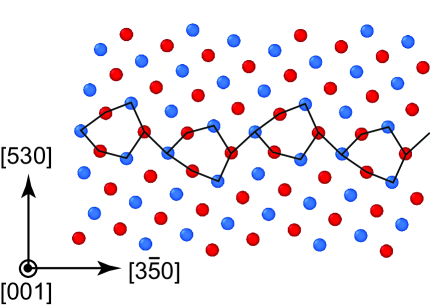
Figure 2: Atomic structure of the $\Sigma 17(530)[001]$ symmetrical tilt GB in Cu. The red and blue circles represent the atoms located in alternating (002) planes normal to the [001] tilt axis. The structural units are outlined.

As a model, we chose the symmetrical tilt $\Sigma 17(530)[001]$ GB with the misorientation angle of $61.93^{\circ}$ ($\Sigma$ is the reciprocal density of coincident sites, [001] is the tilt axis, and $(530)$ is the GB plane). The GB was created in a rectangular simulation block with edges aligned with the Cartesian axes $x$, $y$ and $z$, which in turn were normal to the GB tilt axis, and parallel to the GB tilt axis, and normal to the GB plane, respectively. The block had the approximate dimensions of $6.32\times 6.14\times 80.10$ nm³ and contained $2.64\times 10^{5}$ atoms. The boundary conditions were initially periodic in all three directions. The ground-state structure of this GB is known (Suzuki and Mishin, 2005; Cahn et al., 2006) and consists of identical kite-shape structural units arranged in a zig-zag array as shown in Fig. 2. The GB energy is 856 mJ/m².

A uniform solid solution was created by random substitution of Cu atoms by Ag atoms to achieve the desired alloy composition. The alloy compositions studied here lay within the Cu-based solid solution domain on the Cu-Ag phase diagram. Note that the initial state of the solution did not represent a thermodynamic equilibrium. Under equilibrium conditions, the GB would create a segregation of Ag atoms as was demonstrated in previous work (Frolov et al., 2015, 2016; Hickman and Mishin, 2016; Koju and Mishin, 2020). Furthermore, the solution did not have the correct short range order that forms upon equilibration. The initially uniform random solution was chosen here intentionally in order to observe the process of atmosphere formation during the GB motion. In addition, the formation of short range order was used as an indicator of solute diffusion activated by the GB motion.

The GB was moved by an applied shear strain. The driving force for the motion arises due to the shear-coupling effect (Cahn and Taylor, 2004; Suzuki and Mishin, 2005; Cahn et al., 2006), in which relative translations of the grains parallel to the GB plane cause normal GB motion. Reversely, normal GB motion produces shear deformation of the lattice region traversed by the motion. The shear-coupling effect is characterized by the coupling factor $\beta=v_{||}/v$, where $v_{||}$ is the velocity of parallel translation of the grains and $v$ is the velocity of normal GB motion. For perfect coupling, $\beta$ is a constant that only depends on crystallographic characteristics of the GB. For the particular boundary studied here, the ideal coupling factor is $\beta=-0.496$ (the negative sign reflects the sign convention (Cahn et al., 2006)). To produce GB motion, the boundary condition in the $z$-direction was replaced by free surfaces. The simulation block was re-equilibrated by an MD run in the $NpT$ ensemble (fixed number of atoms $N$, temperature $T$ and pressure $p=0$). Next, the relative positions of the atoms within 1.5 nm thick surface layers were fixed. One bottom layer was fixed permanently, while the other layer was moved, as a rigid body, with a constant translation velocity $v_{||}$ parallel to the $x$-direction. All other atoms remained dynamic. The MD ensemble was then switched to $NVT$ (fixed volume $V$) and the GB was driven in a chosen direction, starting from its initial position at the center of the block, by applying a given translation velocity $v_{||}$.

During the simulations, the GB position was tracked by finding the peak of potential energy of atoms averaged over thin layers parallel to the GB plane. Under perfect coupling conditions, the driving force causing the GB motion equals $P=\beta\tau_{xy}$, where $\tau_{xy}$ is the shear stress parallel to the GB plane (Cahn and Taylor, 2004; Cahn et al., 2006). The latter was computed from the virial equation averaged over the entire simulation block and over time in the steady-state regime. The redistribution of Ag atoms caused by the GB motion was analyzed in detail using the OVITO visualization software (Stukowski, 2010). The simulations were performed at the temperature of 1000 K and alloy compositions varying from pure Cu to the solidus line. The grain translation velocity was varied between 0.01 and 60 m/s. Implementing lower velocities would require computational resources that were not available to us.

III Results

III.1 The solute drag dynamics

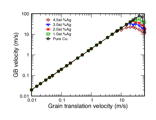
Figure 3: GB migration velocity $v$ as a function of the applied grain translation velocity $v_{||}$. The alloy compositions are indicated in the key.

The ability to predict the driving force using the equation $P=\beta\tau_{xy}$ predicates on the shear coupling being perfect. Our first step was, therefore, to find the conditions under which the coupling factor $\beta$ was close to its ideal value. Fig. 3 shows a typical plot of GB velocity versus the imposed grain translation velocity. At small enough velocities, the relation between $v$ and $v_{||}$ is linear with the slope matching the ideal value of $\beta$. After a critical velocity is reached, the GB shows downward deviations from the ideal behavior. Such deviations were observed previously (Cahn et al., 2006; Mishin et al., 2007) and are usually caused by occasional switches between coupled motion and sliding events. Once the boundary enters this regime, the driving force can no longer be extracted from the shear stress. We thus limited the present simulations to GB velocities below the onset of the downward deviations. For pure Cu, the highest velocity studied was about 40 m/s. For the alloys, the upper bound was lower (10 to 20 m/s), depending on the alloy composition.

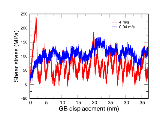
Figure 4: Representative stress-time curves in the Cu-2at.%Ag alloy at two different GB velocities.

Upon application of a grain translation velocity, the shear stress $\tau_{xy}$ initially showed a transient behavior followed by a steady state regime in which $\tau_{xy}$ continued to fluctuate around a constant average value (Fig. 4). The transient time period was somewhat longer for the alloys than for pure Cu. Since the solid solution was initially uniform, time was required to form a dynamic segregation atmosphere surrounding the moving boundary. The shear stresses, and thus the driving forces reported below, were obtained by averaging over a period of time after the onset of the steady state regime.

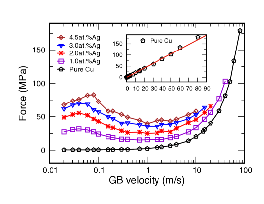
(b)

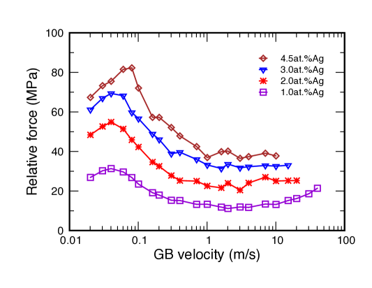
Figure 5: (a) Driving force for GB motion as a function of GB velocity at different alloy compositions. The inset is a zoom into the linear part of the force-velocity relation in pure Cu. (b) The same functions but the driving force in pure Cu has been subtracted from the driving force in the alloys.

The central result of this work is presented in Fig. 5, where the driving force for GB motion is plotted against the GB velocity. Since the GB velocities span three orders of magnitude, they are shown on the logarithmic scale. In pure Cu, the initially linear force-velocity relation becomes highly nonlinear at high velocities. Even though the GB remains perfectly coupled and moves by the same atomic mechanism, the resistance to its motion sharply increases at high velocities. This non-linearity has been seen previously and is caused by a combination of factors, such as (1) faster-than-linear suppression of the energy barrier as a function of the force (Ivanov and Mishin, 2008), and (2) finite rate of heat dissipation by the moving boundary (phonon drag). This nonlinear regime was not considered in the classical model (Cahn, 1962; Lücke and Stüwe, 1963, 1971). In the alloys, the driving force also accelerates in the high velocity limit. However, the force-velocity relation in the alloys is different from that in Cu in two major ways:

• The driving force in alloys is systematically higher than that in pure Cu and increases with the solute concentration. In other words, the driving force required for moving the GB with a given velocity increases with the solute concentration. This solute resistance effect is demonstrated more clearly in Fig. 5b, where the driving force existing in pure Cu has been subtracted from that in the alloys.

• The solute resistance exhibits a maximum at some velocity that increases with the solute concentration. This is precisely the behavior predicted by the classical solute drag models (Cahn, 1962; Lücke and Stüwe, 1963, 1971) (cf. Fig. 1). Thus, on the left of the maximum, the GB is expected to drag of the segregation atmosphere with it, while on the right of the maximum its breaks away from the atmosphere.

The curves presented in Fig. 5 clearly demonstrate that we have been able to reproduce by MD simulations the two modes of the solute resistance to GB motion: both the breakaway mode at high velocities and the solute drag mode at low velocities.

III.2 Direct evidence of solute drag

The fact that the present simulations capture the drag of the solute atoms by the GB can be demonstrated directly by tracking the positions of the solute atoms. One such test is illustrated in Fig. 6 for the Cu-2at.%Ag alloy. Ag atoms (colored in magenta) located in two parallel stripes on either side of the initial GB position were selected for tracking. The GB was driven to the left, eventually passing through the left-hand stripe. The right-hand stripe was not affected by the GB motion and only served as a control region. It was found that the atomic positions in the control region did not practically change, confirming the absence of lattice diffusion on the MD timescale. (To be precise, some atoms did make an occasional jump caused by non-equilibrium vacancies that will be discussed later.) By contrast, the atoms overrun by a slowly moving boundary were randomly scattered due to the accelerated GB diffusion. Importantly, the scattering occurs predominantly in the direction of GB motion, demonstrating that the GB binds the Ag atoms and drags them along over some distance. In other words, the selected Ag atoms are drawn into the dynamics segregation atmosphere traveling together with the boundary. Eventually, they drop out of the atmosphere due to the random diffusive jumps.

The drag effect can be quantified by plotting the final distribution of the Ag atoms in the left-hand stripe after it has been traversed by the boundary as a function of GB velocity and alloy composition (Fig. 7). Each distribution function was obtained by averaging over 20-25 passes of the GB through the stripe. The scatter of the points reflects the limited statistics due to the low solute concentration. The plots demonstrate that, as the GB velocity decreases, the concentration profile becomes increasingly asymmetric and develops a long tail in the low-velocity limit. At the smallest velocity (0.02 m/s), the tail is a factor of 5 longer than the initial width of the stripe. The effect of the alloy composition on the concentration profiles is less significant, which is not surprising given that the alloys are dilute.

For comparison, Fig. 8 shows similar concentration profiles for the host Cu atoms initially residing within the same stripe. At low GB velocities, the Cu profiles broaden and develop an asymmetric $\lambda$-shape. However, the broadening is much smaller than for the Ag atoms and does not contain the long tail in the direction of motion. The degree of broadening does not practically depend on the alloy composition. As shown in the Appendix, the characteristic $\lambda$-shape of the Cu concentration profiles is consistent with purely diffusional broadening caused by accelerated diffusion during the time when the GB is inside the stripe. This type of broadening is not related to solute drag. For Cu atoms, the drag does not exist in pure Cu and is negligible in alloys, where the Cu segregation (to be precise, “anti-segregation”, because the segregated Ag atoms substitute for Cu) is small. The drastic difference between the profile of Ag and Cu (cf. Figs. 7 and 8) confirms that the Ag atoms were subject to a strong drag effect.

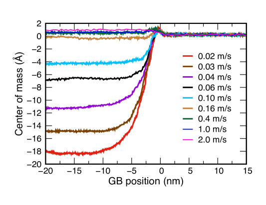
(b)

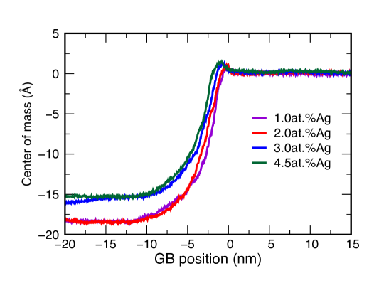
Figure 9: Position of the center of mass of Ag atoms located within a stripe overrun by a moving GB as a function of GB position $z$. The GB moves from right to left with the center of the stripe located at $z=0$. (a) for different GB velocities at a fixed alloy composition (Cu-2at.%Ag); (b) for different alloy compositions at a fixed velocity of 0.02 m/s.

Yet another demonstration of the solute drag was obtained by tracking the $z$-coordinate of the center of mass of the selected atoms. By definition of the solute drag, the GB carries over some distance the center of mass of any group of solute atoms that it overrun during its motion. This was indeed observed at small GB velocities as illustrated in Fig. 9. The center of mass of the Ag atoms located within the selected stripe initially coincides with the center of the stripe ($z=0$). As soon as the moving GB enters the stripe, the center of mass of the Ag atoms starts moving in the same direction. This motion persists for some time after the GB exists the stripe, demonstrating that the Ag atoms continued to travel along with the boundary. Since they also make random diffusive jumps, they gradually drop out the segregation atmosphere and the center of mass eventually stops moving. At slow GB velocities, the net displacement of the center of mass reaches 2 nm, which is at least twice the GB width.

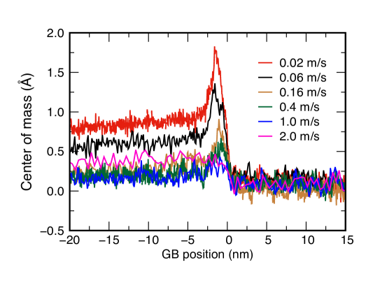
(b)

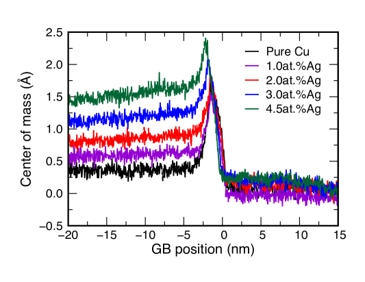
Figure 10: Position of the center of mass of Cu atoms located within a stripe overrun by a moving GB as a function of GB position $z$. The GB moves from right to left with the center of the stripe located at $z=0$. (a) for different GB velocities at a fixed alloy composition (Cu-2at.%Ag); (b) for different alloy compositions at a fixed velocity of 0.02 m/s.

In comparison, the net displacement of the center of mass of the Cu atoms located in the same stripe is drastically smaller (Fig. 10). Even at the lowest GB velocity, the displacement of the center of mass is on the order of 0.1 nm. Note also that the plots in Figs. 9 and 10 display a characteristic local maximum arising when the GB is inside the stripe. This small peak is a manifestation of a subtle diffusion effect that is not related to solute drag. Purely diffusion calculations presented in the Appendix give a similar small displacement of the center of mass, followed by its reversal after the GB exists the stripe. The predicted split of the maximum in two could not be resolved in the present simulations due to statistical errors.

III.3 The role of grain boundary diffusion

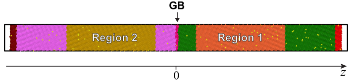
(b)

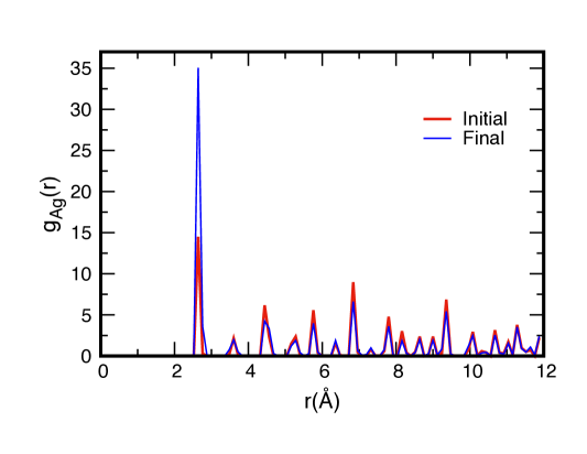
(c)

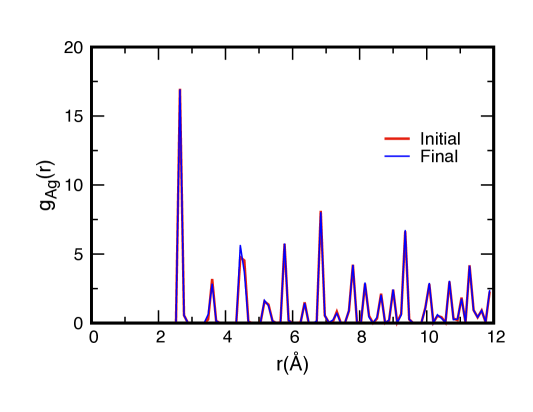
Figure 11: (a) Selection of regions 1 and 2 in the simulation block. Region 1 is traversed by the GB moving to the right starting from the middle of the simulation block, while region 2 is a control region that is not influenced by the GB. (b) and (c) show the final radial distribution functions of Ag atoms in regions 1 and 2, respectively. The alloy composition is Cu-2at.%Ag.

We next demonstrate that a moving GB accelerates diffusion in lattice regions traversed during its motion. As an indicator of lattice diffusion, we choose the change in the short range order in the solid solution. Recall that the Cu-Ag solution was created by random atomic substitution. As such, it initially has zero short range order. Since lattice diffusion is frozen, short range order cannot form. To demonstrate the GB effect on short range order, two regions were selected on either side of the GB (Fig. 11a). The GB starts out in the middle of the simulation block and moves to the right, passing through region 1. Region 2 is not influenced by the GB motion and only serves as a control region. The radial distribution function (RDF) of Ag atoms is monitored in both regions as a function of time.

The initial RDF in both regions is similar to that of a single-component face centered cubic lattice (Fig. 11b,c). The relative positions and heights of the peaks are only dictated by the crystallography. The absolute positions and heights may slightly vary with temperature due to thermal expansion and with chemical composition due to the atomic size difference between Cu and Ag. However, in this work such variations are immaterial because the Ag concentrations are too small and the temperature is fixed. As the GB sweeps through region 1, the peak heights change significantly. In particular, the first peak grows higher, indicating the preference for Ag atoms to become nearest neighbors (Fig. 11b). This clustering trend is consistent with the existence of a wide miscibility gap on the Cu-Ag phase diagram. Meanwhile, no change in the RDF was found in the control region.

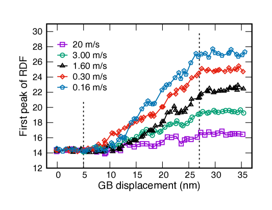
(b)

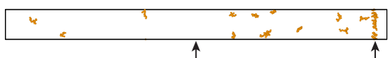
Figure 12: (a) The height of the first peak of the RDF of Ag atoms in the region traversed by the moving GB. The dashed vertical lines outline the boundaries of the region. The alloy composition is Cu-2at.%Ag. (b) Formation of Ag clusters in the region swept by the GB moving in the Cu-4.5at.%Ag alloy with the velocity of 0.04 m/s. Only Ag clusters containing 15 or more atoms are shown, while all other atoms are invisible. The arrows indicate the initial (left) and final (right) GB positions.

In Fig. 12a, the height of the first peak of the RDF averaged over region 1 is plotted as a function of GB position. The plot shows that, as soon as the GB enters the region, the height of the peak begins to rise. The rise continues until the boundary exits the region, after which the height of the peak remains constant. The net change of the peak is small when the boundary moves fast but increases significantly as the GB velocity decreases. For a visual demonstration of the short range order formation, Fig. 12b shows the distribution of Ag clusters in the alloy. A cluster is defined as a group of atoms interconnected by nearest-neighbor bonds. The probability of such clusters in the initial random alloy is nonzero but very small. The image demonstrates the formation of a trail of new clusters containing more than 15 atoms each that were left behind the moving GB. The formation of short range order in region 1 could only occur by diffusive jumps of both Ag and Cu atoms. Thus, the simulations confirm that a GB can activate otherwise frozen diffusion in lattice regions swept by its motion. The slower the motion, the longer is the time spent by atoms in the high-diffusivity GB region, and thus the higher is the effective, GB-induced diffusivity in the lattice.

III.4 Vacancy generation by a moving grain boundary

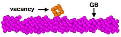
(b)

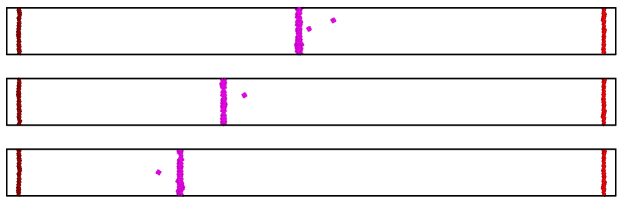
Figure 13: Example of vacancy ejection and absorption during GB motion. (a) The GB moves in the downward direction and the vacancy is at the center of the 12-atom cluster of defected atoms revealed by common neighbor analysis with OVITO (Stukowski, 2010). The GB orientation is the same as in Fig. 2 (b) Sequence of snapshots of a GB moving to the left with the velocity of 0.02 m/s. The dots represent the non-equilibrium vacancies surrounding the GB.

The simulations have also revealed that a moving GB spontaneously emits and re-absorbs vacancies, effectively creating a vacancy atmosphere moving together with the boundary (Fig. 13). The local vacancy concentration in the atmosphere exceeds the equilibrium vacancy concentration in the material.

The equilibrium number of vacancies in the simulation block can be estimated from the equation

$$N_{v}=N\exp\left(-\dfrac{E_{v}}{k_{B}T}\right),$$ (1)

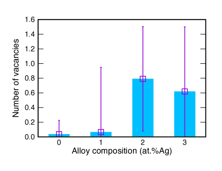
(b)

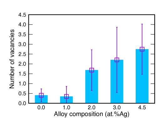
Figure 14: Time-averaged number of vacancies in the simulation block containing (a) stationary GB and (b) moving GB in pure Cu and in Cu-Ag alloys. The GB velocity is 0.02 m/s. The error bars indicate one standard deviation.

where $N$ is the number of atoms in the system, $E_{v}=1.272$ eV is the vacancy formation energy in Cu predicted by the interatomic potential, $k_{B}$ is Boltzmann’s constant, and $T=1000$ K is temperature. From this equation, $N_{v}\approx 0.1$, meaning that the chance of seeing a single vacancy in the simulation block is about 10%. To verify this estimate, MD simulations were performed on a stationary GB in both pure Cu and the alloys at 1000 K. In this setting, the GB serves as a source of vacancies. The time-averaged number of vacancies present in system is shown in Fig. 14a for several chemical compositions. The error bar is large because the system typically contains either one or no vacancy at any given time. In pure Cu, the average number of vacancies is found to be less than 0.1. This number increases in the alloys, reaching about 0.7 at 2-3 at.%Ag.

Fig. 14b shows that a moving GB increases the number of vacancies in both Cu and the alloys, reaching 2 to 3 vacancies at 2 to 4.5 at.%Ag. Visualization of the vacancies reveals that this increase primarily comes from vacancies ejected by the GB into the lattice and returning back to it after a short excursion. Thus, the averaging of the number of vacancies over the entire system strongly underestimates the actual increase in the vacancy concentration near the GB.

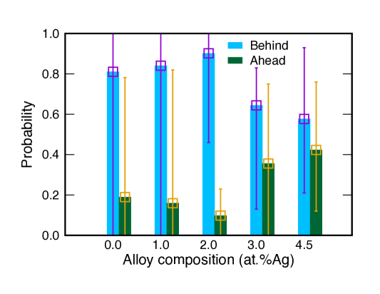
Figure 15: Probability of finding a vacancy ahead or behind the moving GB in the Cu-2at.%Ag alloy. The GB velocity is 0.02 m/s. The error bars indicate one standard deviation.

It was also noticed that the vacancy distribution on either side of the moving boundary was not equal, with more vacancies trailing the GB than jumping ahead of it. This effect is illustrated in Fig. 15 where the probability of finding a vacancy ahead of the moving GB versus in it wake is shown for several alloy compositions. The asymmetry is very significant but tends to decrease with the solute concentration.

IV Concluding remarks

The main conclusion of this work is that it is presently possible to model the solute drag by moving GBs by means of conventional MD simulations. Both the drag and the breakaway kinetic regimes can be reproduced and studied in atomic detail as a function of alloy composition. The two regimes are separated by a maximum of the drag force (Fig. 5) in full agreement with predictions of the classical solute drag model (Cahn, 1962; Lücke and Stüwe, 1963, 1971). This finding opens a research direction in which the solute drag can be investigated with atomic precision without any approximations other than those of the interatomic potential.

Further progress in this direction depends on the availability of reliable interatomic potentials capable of reproducing thermodynamic properties of alloys systems on a quantitative level. Another limiting factor is the computational power. The smallest GB velocity implemented in this work (0.02 m/s) could have been lower if we had access to more advanced computational resources, which are certainly available today. As computers become faster and/or longer MD times become more accessible, it should soon be possible to extend the solute-drag branch of the force-velocity curve (Fig. 5) to lower velocities. It is in that region that some of the most interesting processes can unfold, such as the drag of a heavy, nearly equilibrium, segregation atmosphere by a slowly moving boundary. Furthermore, the cross-section of the GB could be increased to observe the morphological evolution of the moving boundary.

The reason why it is possible to observe the solute drag in spite of the fact that the lattice diffusion is frozen out on the MD timescale is that the accelerated GB diffusion provides enough atomic mobility to allow the solute atoms to follow the moving boundary. GB diffusion is known to be many orders of magnitude faster than lattice diffusion (Kaur et al., 1995; Mishin et al., 2010; Mishin, 2015). A moving GB effectively activates solute diffusion in lattice regions swept during its motion. In this work, it was not possible to quantify this effect directly due to the small solute concentration. However, indirect evidence has been provided by showing that the moving GB creates short range order in the initially random solid solution. Since short range order formation is a diffusion process, it could only be created by activation of diffusive jumps. Under real experimental conditions, lattice diffusion can also contribute to the solute transport toward or away from the moving GB, at least for slow GB motion. This does not change the solute drag process qualitatively but may shift the maximum of the drag force toward higher velocities.

It should be noted that the short range order formation behind a moving GB gives rise to an additional driving force for forward motion. This force is equal to the difference between the free energies of the ordered and disordered states of the solution per unit volume. Attempts were made to evaluate this force by interrupting the GB motion (removing the applied shear stress) and continuing the MD simulation with a stationary GB separating the ordered and disordered lattices. No significant GB motion was observed, indicating the driving force of ordering was too small detect it in this work. But it could, in principle, be one of the factors in microstructure evolution in alloys.

Another effect found in this work is the vacancy generation by a moving GB (Fig. 13). The accepted paradigm is that the fast GB diffusion is localized within the GB core whose width is around 0.5 to 1 nm (Kaur et al., 1995). Hence, lattice atoms can only experience accelerated diffusion when they find themselves inside the core region of the moving boundary. We find that this picture is incomplete. A moving GB drags an atmosphere of non-equilibrium vacancies that enhance the diffusivity in wider lattice regions than the width of the GB core. Spontaneous ejection of vacancies into the lattice and their return to the GB after a short excursion appears to be a general phenomenon. A similar behavior of vacancies was previously found in MD simulations of edge and screw dislocations in Al (Pun and Mishin, 2009).

Although this study was focused on one particular high-angle GB chosen as a model, the phenomena discussed are generic and should be relevant to most GBs to one degree or another. Special low-energy GBs, such as $\Sigma 3$ coherent twin boundaries, may display specific features such as weaker interaction with solutes and/or lower diffusivity. The main conclusions of the work may not be applicable to them without proper modifications.

Acknowledgement: This work was supported by the National Science Foundation, Division of Materials Research, under Award No. 1708314.

Appendix

In this Appendix we provide additional evidence that the profile broadening shown in Fig. 8 is primarily caused by GB diffusion with little or no effect of the solute drag. To this end, we numerically solve the continuous diffusion equation

$$\dfrac{\partial c}{\partial t}=D(z,t)\dfrac{\partial^{2}c}{\partial z^{2}}$$ (2)

with the boundary condition $c(\pm\infty,t)=0$ and the initial condition

$$c(z,0)=\begin{cases}1,&|z|\leq a,\\ 0,&|z|>a.\end{cases}$$ (3)

Here, $c$ represents the concentration of Cu atoms selected within a stripe of width $2a$ located at $z=0$ (cf. Fig. 6). These atoms can be thought of as isotope tracer atoms implanted into the stripe. The diffusion coefficient is given by the moving Gaussian

$$D(z,t)=D_{0}\exp\left[-(z-z_{0}-vt)^{2}\right].$$ (4)

This function represents the enhanced diffusion coefficient in the GB moving with the velocity $v$ starting from its initial position at $z_{0}$. Thus, the diffusion coefficient tends to zero outside the GB and reaches the largest value $D_{0}$ at the center of the boundary. In the calculations shown here, the boundary moves to the left starting from its initial position on the right of the stripe.

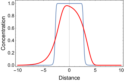
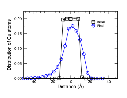
(a)                    (b)

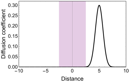
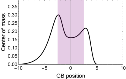
(c)                    (d)

Figure 16: Concentration profiles before and after a moving GB passes through a stripe of tracer atoms. (a) Predicted by the diffusion equation (2) with the dimensionless parameters $a=2$, $z_{0}=5$, $v=-0.3$ and $D_{0}=0.3$. The GB moves from right to left. The initial profile is shown in blue, the final in red. (b) Similar profiles obtained by atomistic simulations in pure Cu for the GB moving with the velocity of 0.02 m/s. (c) The diffusion coefficient for the initial GB position according to Eq.(4). (d) Position of the center of mass of the diffusing atoms as a function of GB position as the latter traverses the stripe. In (c) and (d), the shaded area indicates the stripe containing the diffusing atoms.

Fig. 16a compares the concentration profiles before and after the boundary passes through the stripe, with the diffusion coefficient shown in Fig. 16c. The final shape of the concentration profile is qualitatively similar to the profile observed in the simulations (Fig. 16b). Furthermore, in Fig. 16d we plot the position of the center of mass of the diffusing atoms as a function of GB position. The center of mass shows a small displacement toward the GB when the latter just enters the stripe, slightly retreats while the GB is inside the stripe, and finally moves slightly away from the boundary as the latter exits the stripe. This produces the two peaks observed in the plot. However, once the boundary passes through the stripe, the center of mass returns to its original position. As expected physically, the diffusion process does not produce a net displacement of the center of mass. Indeed, the equations solved here only describe the enhancement of diffusion by the moving boundary and do not include any interaction between the diffusing atoms and the boundary. The temporary displacements of the center of mass are smaller than the GB width and can be neglected for practical intents and purposes.

Thus, the concentration profiles of the Cu atoms observed in the simulations (Fig. 8) are well-consistent with the purely diffusion enhancement by the moving GB without any significant solute drag. The drastic difference between these profiles and those for Ag atoms (Fig. 7), featuring a long concentration tails, confirms that the Ag atoms strongly interact with the moving GB and are dragged by it in the direction of motion.

(a)

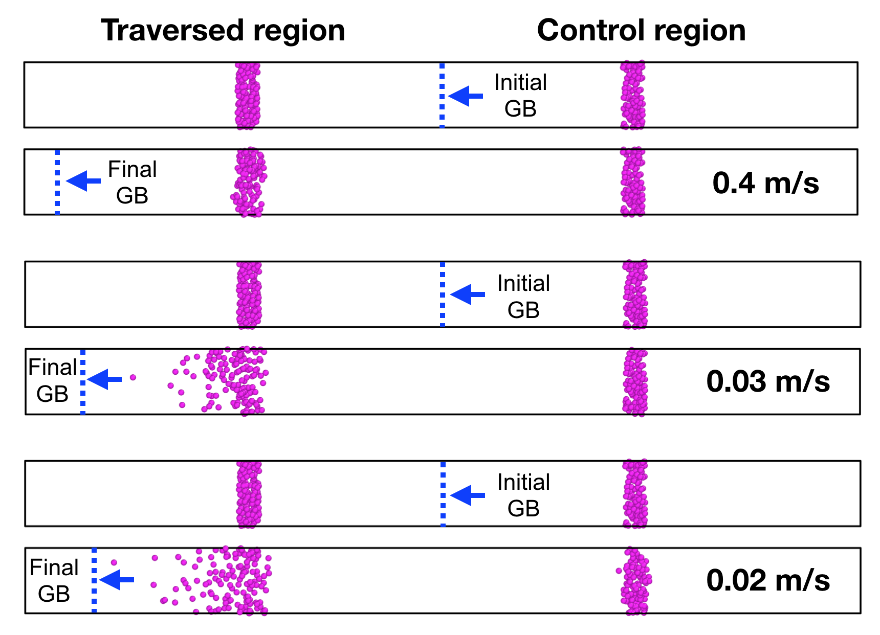
Figure 6: Demonstration of the effect of GB motion on solute distribution. Ag atoms within two 2 nm thick stripes are colored in magenta. The GB moves to the left with the velocity indicated in the legend and crosses the left-hand stripe, scattering the Ag atoms predominantly in the direction of motion. The scattering asymmetry is stronger for the smaller velocity. The right-hand stripe serves as a control region, demonstrating the absence of lattice diffusion. The alloy composition is Cu-2at.%Ag.

(a)

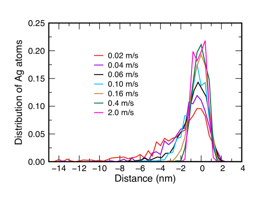
(b)

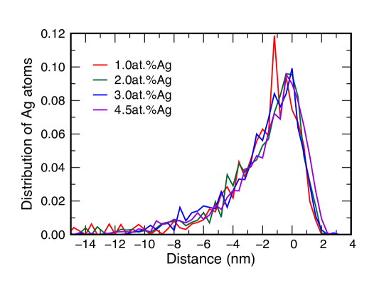
Figure 7: Distribution profiles (normalized to unity) of Ag atoms in the final state of a 2 nm stripe overrun by a moving GB: (a) for different GB velocities at a fixed alloy composition (Cu-2at.%Ag); (b) for different alloy compositions at a fixed velocity of 0.02 m/s. The center of the stripe is at $z=0$.

(a)

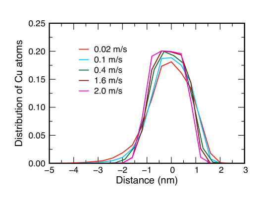
(b)

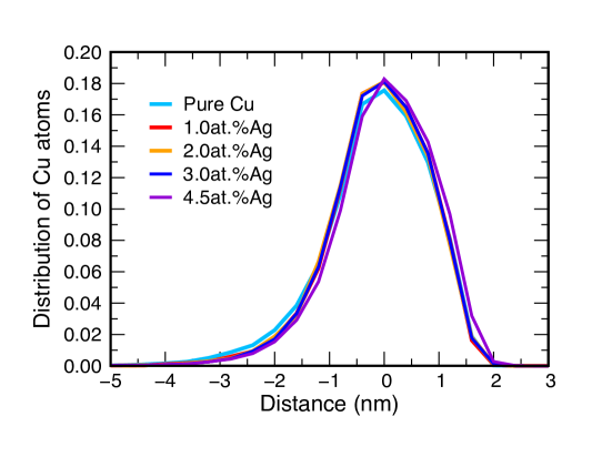
Figure 8: Distribution profiles (normalized to unity) of Cu atoms in the final state of a 2 nm stripe overrun by a moving GB: (a) for different GB velocities at a fixed alloy composition (Cu-2at.%Ag); (b) for different alloy compositions at the fixed velocity of 0.02 m/s. The center of the stripe is at $z=0$.

(a)

(a)

(a)

(a)

(a)

(a)

References

- Sutton and Balluffi (1995) A. P. Sutton, R. W. Balluffi, Interfaces in Crystalline Materials, Clarendon Press, Oxford, 1995.
- Mishin et al. (2010) Y. Mishin, M. Asta, J. Li, Atomistic modeling of interfaces and their impact on microstructure and properties, Acta Mater. 58 (2010) 1117 – 1151.
- Cahn (1962) J. W. Cahn, The impurity-drag effect in grain boundary motion, Acta Metall. 10 (1962) 789–798.
- Lücke and Stüwe (1963) K. Lücke, H. P. Stüwe, On the theory of grain boundary motion, in: L. Himmel (Ed.), Recovery and Recrystallization of Metals, Interscience Publishers, New York, 1963, pp. 171–210.
- Lücke and Stüwe (1971) K. Lücke, H. P. Stüwe, On the theory of impurity controlled grain boundary motion, Acta Metall. 19 (1971) 1087–1099.
- Ma et al. (2003) N. Ma, S. A. Dregia, Y. Wang, Solute segregation transition and drag force on grain boundaries, Acta Mater. 51 (2003) 3687–3700.
- Li et al. (2009) J. Li, J. Wang, G. Yang, Phase field modeling of grain boundary migration with solute drag, Acta Mater. 57 (2009) 2108–2120.
- Shahandeh et al. (2012) S. Shahandeh, M. Greenwood, M. Militzer, Friction pressure method for simulating solute drag and particle pinning in a multiphase-field model, Model. Simul. Mater. Sci. Eng. 20 (2012) 065008.
- Grönhagen and Agren (2007) K. Grönhagen, J. Agren, Grain-boundary segregation and dynamic solute drag theory — A phase-field approach, Acta Mater. 55 (2007) 955–960.
- Abdeljawad et al. (2017) F. Abdeljawad, P. Lu, N. Argibay, B. G. Clark, B. L. Boyce, S. M. Foiles, Grain boundary segregation in immiscible nanocrystalline alloys, Acta Mater. 126 (2017) 528–539.
- Greenwood et al. (2012) M. Greenwood, C. Sinclair, M. Militzer, Phase field crystal model of solute drag, Acta Mater. 60 (2012) 5752–5761.
- Mendelev and Srolovitz (2002) M. I. Mendelev, D. J. Srolovitz, Impurity effects on grain boundary migration, Model. Simul. Mater. Sci. Eng. 10 (2002) R79–R109.
- Sun and Deng (2014) H. Sun, C. Deng, Direct quantification of solute effects on grain boundary motion by atomistic simulations, Comp. Mater. Sci. 93 (2014) 137–143.
- Wicaksono et al. (2013) A. T. Wicaksono, C. W. Sinclair, M. Militzer, A three-dimensional atomistic kinetic Monte Carlo study of dynamic solute-interface interaction, Model. Simul. Mater. Sci. Eng. 21 (2013) 085010.
- Mendelev et al. (2001) M. I. Mendelev, D. J. Srolovitz, W. E, Grain-boundary migration in the presence of diffusing impurities: simulations and analytical models, Philos. Mag. 81 (2001) 2243–2269.
- Rahman et al. (2016) M. J. Rahman, H. S. Zurob, J. J. Hoyt, Molecular dynamics study of solute pinning effects on grain boundary migration in the aluminum magnesium alloy system, Metall. Mater. Trans. A 47 (2016) 1889–1897.
- Kim and Park (2008) S. G. Kim, Y. B. Park, Grain boundary segregation, solute drag and abnormal grain growth, Acta Mater. 56 (2008) 3739–3753.
- Mishin (2019) Y. Mishin, Solute drag and dynamic phase transformations in moving grain boundaries, Acta Mater. 179 (2019) 383–395.
- Williams et al. (2006) P. L. Williams, Y. Mishin, J. C. Hamilton, An embedded-atom potential for the Cu-Ag system, Modelling Simul. Mater. Sci. Eng. 14 (2006) 817–833.
- Plimpton (1995) S. Plimpton, Fast parallel algorithms for short-range molecular-dynamics, J. Comput. Phys. 117 (1995) 1–19.
- Suzuki and Mishin (2005) A. Suzuki, Y. Mishin, Atomic mechanisms of grain boundary diffusion: Low versus high temperatures, J. Mater. Sci. 40 (2005) 3155–3161.
- Cahn et al. (2006) J. W. Cahn, Y. Mishin, A. Suzuki, Coupling grain boundary motion to shear deformation, Acta Mater. 54 (2006) 4953–4975.
- Frolov et al. (2015) T. Frolov, M.Asta, Y. Mishin, Segregation-induced phase transformations in grain boundaries, Phys. Rev. B 92 (2015) 020103(R).
- Frolov et al. (2016) T. Frolov, M. Asta, Y. Mishin, Phase transformations at interfaces: Observations from atomistic modeling, Current Opinion in Solid State and Materials Science 20 (2016) 308–315.
- Hickman and Mishin (2016) J. Hickman, Y. Mishin, Disjoining potential and grain boundary premelting in binary alloys, Phys. Rev. B 93 (2016) 224108.
- Koju and Mishin (2020) R. K. Koju, Y. Mishin, Relationship between grain boundary segregation and grain boundary diffusion in Cu-Ag alloys, Phys. Rev. Materials 4 (2020) 07340.
- Cahn and Taylor (2004) J. W. Cahn, J. E. Taylor, A unified approach to motion of grain boundaries, relative tangential translation along grain boundaries, and grain rotation, Acta Mater. 52 (2004) 4887–4998.
- Suzuki and Mishin (2005) A. Suzuki, Y. Mishin, Atomic mechanisms of grain boundary motion, Mater. Sci. Forum 502 (2005) 157–162.
- Stukowski (2010) A. Stukowski, Visualization and analysis of atomistic simulation data with OVITO – the open visualization tool, Model. Simul. Mater. Sci. Eng 18 (2010) 015012.
- Mishin et al. (2007) Y. Mishin, A. Suzuki, B. Uberuaga, A. F. Voter, Stick-slip behavior of grain boundaries studied by accelerated molecular dynamics, Phys. Rev. B 75 (2007) 224101.
- Ivanov and Mishin (2008) V. A. Ivanov, Y. Mishin, Dynamics of grain boundary motion coupled to shear deformation: An analytical model and its verification by molecular dynamics, Phys. Rev. B 78 (2008) 064106.
- Kaur et al. (1995) I. Kaur, Y. Mishin, W. Gust, Fundamentals of Grain and Interphase Boundary Diffusion, Wiley, Chichester, West Sussex, 1995.
- Mishin (2015) Y. Mishin, An atomistic view of grain boundary diffusion, Defect and Diffusion Forum 363 (2015) 1–11.
- Pun and Mishin (2009) G. P. P. Pun, Y. Mishin, A molecular dynamics study of self-diffusion in the cores of screw and edge dislocations in aluminum, Acta Mater. 57 (2009) 5531–5542.