Abstract

Markov Decision Processes (MDPs) provide important capabilities for facilitating the dynamic adaptation and self-optimization of cyber physical systems at runtime. In recent years, this has primarily taken the form of Reinforcement Learning (RL) techniques that eliminate some MDP components for the purpose of reducing computational requirements. In this work, we show that recent advancements in Compact MDP Models (CMMs) provide sufficient cause to question this trend when designing wireless sensor network nodes. In this work, a novel CMM-based approach to designing self-aware wireless sensor nodes is presented and compared to Q-Learning, a popular RL technique. We show that a certain class of CPS nodes is not well served by RL methods, and contrast RL versus CMM methods in this context. Through both simulation and a prototype implementation, we demonstrate that CMM methods can provide significantly better runtime adaptation performance relative to Q-Learning, with comparable resource requirements.

1 Introduction

This paper presents a novel algorithm and a detailed application of techniques that enable the fast and efficient use of Markov Decision Processes (MDPs) in real-time on resource constrained Cyber Physical Systems (CPSs). By a resource-constrained CPS, we mean distributed systems containing components that have embedded computers whose physical resources are constrained to be significantly below what is available in a typical, consumer-grade desktop or laptop computing system. These limits are typically imposed in order to reduce the size, weight and power, as well as cost (SWAP-C) of each unit. While this is a relative definition of a resource-constrained CPS, what we mean in terms of present technology are embedded systems that would typically have less than 1MB of RAM, less than 10MB of non-volatile storage, and a single-core microcontroller with a clock speed under 100MHz.

MDPs can be used to control computing systems at runtime in ways that are more dynamic, robust and adaptable than alternatives. Using MDPs, engineers can create systems that effectively learn and reason using models of their own system dynamics, observations of their own inherent limitations and effectiveness of their actions towards reaching application-level goals. In this context, these systems exhibit a level of self-awareness in their behavior, with the ultimate design goals being continual autonomous optimization that leads to higher levels of runtime resiliency, robustness and efficiency.

When seeking to develop self-aware systems, researchers have recently turned to Reinforcement Learning (RL) [1], a sub-field of Machine Learning that uses MDPs. However, we believe that there is an important class of CPSs that are not well served by current RL techniques. Specifically, this class of systems is one where some components of the system’s dynamics are known at design time, and the rest are unknown at design time or expected to be time-varying at runtime.

In general, RL frameworks do not try to learn the effect that control outputs have on the system’s state. Instead, they seek to use runtime observations to find a relationship between control outputs and rewards. In general, however, a critical part of this relationship is how the control output affects the state of the system being modeled. In RL frameworks, this causality is implicit in the modeling abstraction and not defined nor learned explicitly. This method works well in many cases, for example in large systems where the state dynamics are too large and complex to be considered or modeled explicitly. However, in this work, we show that departing from this conventional method can be useful for resource-constrained CPSs that have more manageable state spaces. In particular, if engineers possess a priori knowledge about how some of the control outputs might affect the system state, it can be advantageous to codify that knowledge into the learning algorithms at design time. The approach proposed in this work provides models and algorithms that enable designers to exploit a priori knowledge in this way.

Motivated by this deficiency in RL, we define an alternative class of MDP-based system modeling techniques, which we refer to as Compact MDP Models (CMMs), and we develop CMM-based approaches as an alternative to RL for design and implementation of adaptive CPSs. In general, we envision that certain CPSs are better suited for RL, while others are better suited for CMM. Through this work, we seek to explore the causes of why one of these two approaches might be better over another for a given application, and to improve understanding to allow designers to pick the better option.

This paper builds upon a preliminary version in [2], and contributes the following additional content:

• A detailed survey of techniques from the literature that enable the compact use of MDPs on resource constrained systems. This survey leads us to define the class of CMM methods, which encapsulates several different approaches that are useful in streamlining the application of MDPs to CPS systems.

• The introduction of the Sparse Value Iteration (SVI) algorithm — a variation of the SPVI algorithm presented in  [2]. While SPVI is a parallel processing algorithm developed for GPUs, in this work we present a scaled down variation that runs effectively on small, single-threaded Microcontrollers (MCUs).

• A detailed example of how to apply MDP-based techniques to design a wireless sensor CPS.

• The results of a performance simulation, illustrating the differences between a CMM-based design approach compared to Q-Learning, a popular alternative technique from the Reinforcement Learning (RL) literature.

• An empirical study of an MDP solver running on a resource-constrained MCU, including measurements of data storage requirements, execution time and power consumption.

• A power consumption model for an LTE-M wireless modem, derived from experimental lab measurements taken on a live wireless Internet Protocol (IP) data network.

The remainder of the paper is organized as follows. We provide a cursory review of the history of techniques for controlling CPSs in Section 2. In Section 3, we provide a survey of recent advancements in CMMs. In Section 4, we present Structured Learning with Sparse Value Iteration, our novel method for CMM-based design. In Section 5, we detail a case study of a wireless sensor CPS, and explore the challenges and trade-offs inherent in creating an efficient control policy. In Section 6, we illustrate how CMMs can be used to solve the design problem introduced in Section 5 and compare that approach to a competing RL-based approach. Finally, in Section  7 we simulate the runtime performance and in Section 8 we present the results of an embedded system implementation of the competing techniques. We conclude in Section 9 with a discussion of the results and directions for future work.

2 Background and Related Work

The design of algorithms to control resource-constrained computing systems effectively at runtime has been a topic of active research for at least 20 years. A good survey for early work in this area can be found in [3]. This survey reviews a wide range of techniques, including fixed threshold-based approaches, dynamic approaches including stochastic controllers using dynamic programming, as well as some guidance on how MDPs can be used in this context.

Since the time period when that survey was written, a variety of approaches to this research problem has flourished over the years. Some researchers have sought to formulate the design challenge as a constrained optimization problem [4]. Other researchers focused on modeling the dynamics of the system’s energy consumption, and simplifying the control decisions to be simple threshold-based comparisons with respect to the energy budget (e.g., see  [5, 6]). Another popular approach has been to model the system as linear in the context of feedback control systems and then use Model Predictive Control (MPC) theory to modulate a processing duty cycle (e.g.,  [7, 8]).

All of these approaches were shown to be successful in their respective case studies, but share some common limitations when considered for use in other cases. For example, several of these approaches assume deterministic behavior from the system under test. These approaches model the behavior of the system in response to some actuation, and assume the system will always behave the same way. However, many CPSs have some stochastic behavior, either due to complex unmodeled dynamics or due to being affected by an external factors that are difficult to predict. A second common limitation is the assumption that the system being controlled can be modeled as a linear system. Computing systems often do not behave in linear ways, and attempts at formulating linear approximations to non-linear behavior is limited to only the simplest non-linearities, which significantly constrains the overall applicability and generality of this approach. A third common limitation is that the dynamics of the system being controlled often need to be well understood at design time. For many computing systems whose behaviors depend heavily on external factors, this can be an unrealistic assumption.

As efforts in this area progressed, the paradigms shifted from classical control systems theory to various forms of adaptive algorithms, and then to more generalized approaches that researchers have termed as self-configuration, self-optimization and most recently, self-awareness [9]. A wide ranging survey of these works and organization of them into these various self-X categories can be found in [10]. In that work, researchers define self-awareness as “attributes in a system that enable it to monitor its own state and behavior, as well as the external environment, so as to adapt intelligently”. Another definition can be found in [11]$\colon$ “self-aware computing describes a novel paradigm for systems and applications that proactively maintain knowledge about their internal state and its environment and then use this knowledge to reason about behaviours”.

Among the most promising directions for creating these self-awareness attributes in CPSs is through the use of MDPs. MDPs have shown success in this area because they are inherently capable of modeling stochastic behavior and non-linear responses, and they are also well equipped to deal with incomplete models and uncertainty.

2.1 Markov Decision Processes

MDPs provide a generic decision making framework that uses abstract concepts including states, actions, transition probabilities and rewards. Once these concepts are defined they are then passed to an MDP solver, which is an algorithm that produces an optimal policy with respect to those definitions. The policy is a mapping from states to actions, such that an agent using the policy looks up what action to take for any given state.

However, there is no consensus in the literature regarding exactly how to map elements of computing systems to components in the MDP framework. This mapping is in general left to the designer who is applying the MDP to solve a specific computing problem. For example, a processing system can be commanded to run a particular algorithm (and this can be modeled as a state), or that same command can be modeled as an action instead, or it could be modeled as both (an action that leads to a state). Also, the choice of granularity for these definitions is important — e.g., are two invocations of the same algorithm with a slightly different parameter value considered two different actions, or the same action?

There are several approaches in the literature to map elements of computing systems to MDP states and actions, and these different approaches lead to different results, with implications in both the final policy performance as well as how hard it is to model and solve the MDP. One of the earliest known applications of using an MDP to control resources in computing systems at runtime is [12]. Other notable examples of differing approaches in the literature include a reconfigurable router [13], a reconfigurable digital filter bank [14, 15], a power management module for a microprocessor [16], and a smartphone scheduling program that synchronizes email efficiently [17].

2.2 MDP Solvers

One of the first challenges associated with using MDPs is choosing what constitutes a state, an action and a reward. After that is decided, the associated MDP data structures must be stored on a computer and used as the inputs to the MDP solver to produce a policy. With this policy, the runtime decision framework consists of observing what state the system is in, and using that as input to the policy to determine what action to take.

The classical methods to solve MDPs are algorithms known as Value Iteration, Policy Iteration and Modified Policy Iteration [18]. All of these algorithms produce an optimal solution to the MDP problem, with different approaches leading to different implications in the execution time, power requirements and memory use of the solver routines.

These classical MDP solver algorithms suffer from the same issue as most systems that try to reason using computations of probability distributions: the framework’s data structures grow exponentially with the size of the state space. A large state space is desirable in order to have sufficient model expressiveness to tackle difficult decision problems, but this desire is at odds with the resource requirements needed to solve an MDP that has a large state space. The upper limits on memory consumption that are available on typical embedded computing systems can often easily be reached, before many important system details have been modeled.

More specifically, the total number of elements in an MDP’s State Transition Matrices (STMs) is ${{N_{S}^{2}}}N_{A}$, where $N_{S}$ and $N_{A}$ are the number of elements in the state space and action space, respectively. The STMs are the largest data structures in the MDP, and usually the most difficult structures to store and process, due to their large size. The STMs are large matrices even for modest choices of $N_{S}$ and $N_{A}$, and if one were to add a state variable with $L$ states to the state space, this addition would increase the size of the STMs by a factor of $L^{2}$. Besides the storage space and memory requirements to store large data structures, increasing the state space also causes the solver’s execution time and power consumption to grow exponentially as well.

Thus, for CPSs that operate under strict resource constraints, it is not enough to frame an MDP in a way that produces a well performing solution. There is also the practical issue of whether the solver can be successfully implemented on the targeted platform, and whether it can complete in an amount of time reasonable for the application.

This so-called curse of dimensionality [19] usually results in limiting the use of MDPs to a mode of deployment that greatly hampers their usefulness: the solver is invoked only once offline, and then the generated MDP policy only (not the entire framework required to solve the MDP) is used on the target system. This scenario is suboptimal and limiting if the problem inputs are unpredictable, constantly changing, or dependent on the environment. We are interested in the more challenging problem of solving the MDP on demand at runtime, which results in a more intelligent and adaptive class of embedded systems, which can learn, adapt and autonomously re-optimize themselves for changing conditions and use cases.

To overcome the limitations of MDPs with this goal in mind, two main approaches have been pursued: RL and CMMs. RL essentially tries to arrive at the policy without explicitly modeling all of the MDP components or invoking a solver. On the other hand, CMMs are approaches that do define all of the MDP components and invoke a solver, but do so via algorithmic optimizations that significantly reduce computational requirements. These two alternatives are sometimes referred to as model-free and model-based RL, respectively. Henceforth in this paper, when we write “RL”, we refer to model-free RL unless otherwise stated.

We discuss these two categories — RL and CMM — of techniques in Section 2.3 and Section 3, respectively.

2.3 Reinforcement Learning

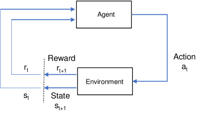
Figure 1: Block diagram of reinforcement learning paradigm.

Reinforcement Learning (RL)  [1] is an area of machine learning that enables systems to formulate optimal decision policies using observations of rewards that are received for previous decisions at runtime. These techniques use MDPs as the framework for formulating the decision problem, but seek to learn the optimal policy directly using observations of rewards in response to decisions, rather than through the explicit definition of all of the MDP components followed by invocation of an MDP solver.

More specifically, an RL framework typically contains the top level block diagram shown in Figure 1. The learning takes place by some agent, which is responsible for selecting an action out of a set of actions, given a system state. This selection is usually done in a discrete-time setting and iterated at a fixed rate. Each selected action (in a given state) leads to some consequence in the environment, and that causes it to transition into a new state in the state space. The selected action and transition to that new state are associated with a scalar reward, which is fed back to the agent (positively or negatively). The agent in turn considers the reward it has been given along with the new state that resulted, and again selects the next action, repeating indefinitely.

As mentioned in the previous Section, these techniques are sometimes referred to as model-free learning. Model-free learning techniques possess the advantage of completely bypassing the need to maintain large STMs, and run computationally intensive MDP solvers.

However, this advantage comes at a cost, as the consequences of all actions taken in all states have to be learned and constantly validated, even those that are constant and known a priori at design time. This learning comes at the cost of occasionally having to make random decisions at runtime to explore the effect of alternative decisions[20]. This cost is a central drawback of model-free techniques, and is associated with a complex trade-off called the exploration versus exploitation trade-off [1].

One popular RL technique that has shown promising results is Q-Learning [16, 21, 22, 23]. In Q-Learning, a scalar value “Q” is assigned to each action in each state, and referred to as the Q-Function. This function represents the average future rewards that can be expected by taking a given action in a given state. The Q-Learning method continually learns and updates this Q-Function using a simple technique called the method of Temporal Differences (TD)  [24], and uses it to formulate an optimal control policy that is based entirely on the system and environment involved. As the environment and the system’s dynamics change at runtime, the policy changes with it.

In one example [16], an Adaptive Power Management (APM) hardware module using Q-Learning was used to put a microcontroller in and out of low power states, and resulted in a learning controller that managed power transitions better than an expert user. In another example [21], Q-Learning was used to optimize the throughput of an energy harvesting wireless sensor node while meeting challenging constraints.

In the next section, we give an overview of CMM methods, which can be viewed as model-based RL methods that are designed with an emphasis on streamlining computational efficiency. We survey recent advancements in this area that result in performance on par with Q-Learning.

3 Survey of Compact MDP Models

As mentioned in the previous section, the deployment of MDPs in resource-constrained systems has typically been limited to usage modes where the MDP modeling and solving are done offline, and only the resulting policy is stored in the runtime system. The goal of moving the MDP model and solver into the runtime system by mitigating the longstanding barriers has been a common goal among many researchers over the years, resulting recently in very creative and effective techniques. We refer to this category of approaches as compact MDP models (CMMs), given that they provide a smaller or computationally optimized representation of the system in question than compared to a direct implementation of the MDP’s data structures. The effectiveness of these recent developments, especially when applied in combination with one another, leads us to question the conventional approach of limiting consideration to model-free RL approaches in the implementation of resource-constrained, MDP-based systems.

Some of these CMM techniques seek to reduce the storage size of the MDP’s data structures by exploiting some structural component embedded within the MDP (e.g., see [2, 25, 26, 27, 28]). Other techniques involve modeling approaches that reduce the MDP state space via generalization and abstraction of system dynamics (e.g., see [14, 15]). Another approach has been to keep algorithms and data structures as is, and take advantage of recent advancements in parallel processing using embedded GPUs, for example  [29, 2].

In our case study, we utilize three CMM techniques: factorization, exploitation of sparsity, and transition states, and we show the significant advantages that they provide when compared to both a direct classical MDP implementation and a competing model-free method. In the remainder of this section, we present an overview of four important CMM techniques from the literature, including the three techniques that are used in our case study. One of the techniques surveyed here — hierarchical decomposition — is not used in our case study, but still presented here due to its importance and widespread use in the field.

3.1 Factorization

In MDP problems, the state $s\in\mathcal{S}$ is constructed to model the problem the MDP is being applied to. Often this results in the state being an instantiation of a discrete multivariate random variable $\underline{Z}=(Z_{1},Z_{2},\ldots,Z_{N_{Z}})$, with each variable $Z_{i}$ taking on values in $\mathit{DOM}(Z_{i})$, where $\mathit{DOM}(X)$ represents the set of admissible values of the random variable $X$. A state is a set of instantiations of the $N_{Z}$ random variables, and can be written as a vector $\underline{z}\in\mathit{DOM}(\underline{Z})$. The size of the state space is defined by the cardinality of this set, which we denote as $\left|{\mathit{DOM}(\underline{Z})}\right|$. As a result, each row of each transition matrix for an MDP has width $\left|{\mathit{DOM}(\underline{Z})}\right|$, and describes the probability of reaching all possible combinations of the set of variables $(Z_{1},Z_{2},\ldots,Z_{N_{Z}})$.

We refer to MDPs with this kind of formulation as having a multivariate state space. When an MDP’s STMs are stored in a structured way that uses knowledge of the causal relationships between these state variables to reduce storage size, the MDP is said to be factored. To the best of our knowledge, the earliest publication detailing the concept of factored MDPs is Boutilier et al. in [25]. These researchers proposed factored MDPs as a method for compact representation of large, structured MDPs. Through application and empirical observations, we have found that this method can effectively reduce STM storage size considerably. However, it requires a specific conditional probability structure to be present in an MDP, and the data structures must be created by hand with specific knowledge of the exact structure. This can require a subject matter expert in the loop anytime a transition probability changes, which can complicate runtime autonomous solving of an MDP that changes over time in unknown ways. In general, this requirement can be problematic if the underlying structure is not fully understood. We acknowledge the effectiveness of the technique, but also the fact that it cannot always be used.

We applied this technique in  [2] where we used a factored MDP to create a control policy for a reconfigurable digital filter bank. Factoring the MDP resulted in a reduction of the number of elements in the STM from $121.8x10^{6}$ to $66.3x10^{3}$. This is a very important reduction, because a matrix with 66k elements can realistically be stored in a low power MCU, whereas one with 121M elements typically cannot.

With the goal of creating a custom solver that works directly on a factored MDP, Hoey et al.  [26] detail an algorithm similar to Value Iteration that can solve MDPs in factored form using Algebraic Decision Diagrams. This approach shows good results in taming the curse of dimensionality, but imposes the same restrictions as [25] and thus has the same limitations. Additionally, the state transition matrices must be manually converted into tree-shaped conditional probability structures, which we found to be considerably difficult and time-consuming.

3.2 Hierarchical Decomposition

In  [27], Jonsson and Barto present an algorithm that performs hierarchical decomposition of factored MDPs into smaller subtasks to help alleviate the growth in complexity that follows from a modestly-sized state space. This approach can be effective, but also requires a priori knowledge of the causal structure within the MDP. This knowledge can be very difficult or impossible to know for many MDPs, a shortcoming identified by the authors themselves. Also, this method requires that the MDP have this decomposability property, which is not always the case.

In a similar spirit, Lin and Dean [28] present a method to solve a large MDP by first decomposing the state space into regions, determining actions to take within those regions, and then using novel approaches to combine the resulting sub-policies into an overarching policy that solves the original, large MDP. The authors note in this work that the decomposition must be done a priori by a domain expert. This decomposition is not guaranteed to be feasible, and when it is feasible, it can be very difficult to perform.

3.3 Sparsity

Another approach in reducing the computational requirements of MDPs is the exploitation of the sparsity typically found in the MDP data structures. In this context, we refer to sparsity as a high percentage of zero-valued elements in the MDP STMs. A discussion on the reasons why sparsity typically results in MDPs can be found in [2]. In [30], Wijs et al. present a promising method to decompose MDPs into subgraphs, exploiting sparsity on GPUs. However, the method is presented in the context of model checking for formal methods in software engineering. More research is required to incorporate this method into an MDP solver.

In  [2], we introduced Sparse Parallel Value Iteration (SPVI), an MDP solver algorithm that exploits sparsity through a three-step process: 1) an algebraic manipulation of the MDP components is performed that combines the multiple STMs into a single large matrix, 2) the large matrix is stored in a sparse matrix format, and 3) a specialized form of the Value Iteration algorithm is used to operate on the MDP directly in this transformed state. The examples in [2] detailed significant improvements in both storage requirements and solver computation time, however that work also exploited parallelism in GPUs to achieve this result. In Section 8, we show that the sparse linear algebra techniques are also quite effective when running on a resource constrained single threaded MCU, not just on the much more powerful processing environment (including hundreds of parallel threads) provided by GPUs. When running in a single threaded CPU, we no longer have any parallel processing and thus refer to the algorithm more simply as Sparse Value Iteration (SVI). We believe that our SPVI and SVI solvers are the first reported MDP solver implementation (either CPU- or GPU-based) that exploit sparsity to make significant performance gains in both storage requirements and computation time.

3.4 Transition States

In [14], we introduced the concept of transition states, which is based on a similar concept initially proposed in [12]. We expanded and elaborated on the initial concept in both [14, 15].

In our design context in this paper, the system being controlled contains many discrete states. Depending on the level of modeling and decision making that is desired, as much as tens of thousands of states or more could be considered relevant. In general, the modeling process involves making design-time decisions as to what level of detail is modeled in the MDP, for each of the system characteristics and dynamics. More fine-grained detail allows for a more precise model, but this leads to a large state space and the computational challenges associated with that.

The concept of transition states allows for significant reduction of the state space to occur when the system passes through a large set of states for a limited time, and the only relevant detail is when the system enters and exits the set as a whole. In some way, these trajectories need to be modeled in the MDP. By utilizing the concept of transition states, large groups of fine-grained states are abstracted away into a single coarse-grained state referred to as a transition state. While the system is actually in one of the many fine-grained states, the system is modeled as being in transition through the single coarse-grained transition state. The transition state encapsulates a set of discrete states that are present but not relevant to the decision process being designed. The only transition probability needed is derived from an estimate of the expected time until the system leaves the set of states. A discussion on how to apply this to stochastic dynamics, and some of the trade-offs associated with this concept can be found in  [14, 15].

4 Method

4.1 Structured Learning

Creating an MDP model on a computing system consists of defining the states and actions, the STMs, and the reward function for the given decision problem and its environment. The STMs are $N_{A}$ stochastic matrices, each of size $N_{S}$ by $N_{S}$ (one matrix for each action). Each STM defines the probability of transitioning from the current state to any one of the possible other states, given an action. We generally write this as a discrete conditional probability distribution as in Equation 1:

$$p(s^{(n+1)}|s^{(n)},a^{(n)}),\forall s\in\mathcal{S},a\in\mathcal{A},$$ (1)

which gives the probability of the system transitioning to state $s^{(n+1)}$ at time index $n+1$ given that it was in state $s^{(n)}$ and action $a^{(n)}$ was selected at time index $n$. The process of instantiating the STMs is the allocation of storage for ${{N_{S}^{2}}}N_{A}$ numerical quantities and assigning them values from 0 to 1. Given this viewpoint, we group the methods in the literature into two categories: the model-based approach where all $N_{A}{N^{2}_{S}}$ terms are defined a priori and treated as constants, and the model-free approach, where none of the ${{N_{S}^{2}}}N_{A}$ are defined and in fact storage for them is never even allocated.

In this paper, we view these as two extremes of a continuum that has many other options. We propose a blend between the two, where some of the STM terms are assumed to be known a priori, and others are not. More specifically, we define:

$$\begin{split}p(s^{(n+1)}|s^{(n)},a^{(n)})\in\{\Gamma\cup\hat{\Theta}\},\\ \forall s\in\mathcal{S},a\in\mathcal{A},\end{split}$$ (2)

where we imply that all of the probability values in the STMs come from one of two parameter subsets $\Gamma$ and $\Theta$. The set $\Gamma$ is the set of STM entries that are fully known a priori and can be set to a fixed value at design time. The set $\hat{\Theta}$ contains the remaining matrix elements; they are either not known a priori or are expected to be time-varying at runtime. We use $\hat{\theta}$ to denote the latest value of a running of estimate of the true value, for each parameter $\theta\in\Theta$.

Rather than taking the entire STM as either constant, or completely unknown, we adopt a flexible middle ground and assume it to be partially known and partially unknown. In this way, the system model has some parts of it that are fixed, and other parts that are assumed to change over time. Then, the runtime adaptation process consists of learning only the set of parameters $\hat{\Theta}$, rather than the entire STM. In this way, the model contains a mix of some predetermined structure from $\Gamma$) and some online learning (from $\hat{\Theta}$). We refer to this approach as Structured Learning.

Structured Learning allows us to restrict how much effort is spent trying to learn unknown parameters, and results in higher overall awareness and adaptation performance for a certain class of CPS devices, as will be demonstrated in our case study. The advantage comes from being able to direct the system’s learning efforts to be focused on the relevant parts of the problem, and prevent redundant attempts to constantly question and re-visit assumptions about the system that a system designer knows will never change.

4.2 Temporal Difference Equations

The Structured Learning method defined above relies on a continual online learning of parameters. For this, we use a very simple technique prevalent in RL: the use of weighted averaging through Temporal Difference (TD) equations, with the central concept shown in Equation 3:

$$\hat{\theta}^{(n+1)}=\hat{\theta}^{(n)}\cdot(1-\alpha)+\theta^{(n)}\cdot\alpha,$$ (3)

where $\theta^{(n)}$ is an observed value of one of the parameters $\theta\in\Theta$ at timestep $n$, $\hat{\theta}^{(n)}$ is the value of the running estimate of $\theta$ at timestep $n$, and $\alpha$ is a learning rate parameter which controls how sensitive the running estimates are to individual observations. The method essentially consists of performing a low-pass filtering or smoothing operation on observed values, and thus maintaining a running estimate that tracks the latest observed values for a given parameter.

As the observations change over time, the running estimates track the changes while also reducing the effect of statistical outliers. Using TD, the Structured Learning method can ingest the latest observations of each of the parameters $\theta\in\Theta$, compute the running set of estimates for each $\hat{\Theta}$, and combine them with the constant set $\Gamma$ to assemble the fully populated, partially time-varying STMs at any timestep.

4.3 Sparse Value Iteration (SVI)

In Structured Learning we instantiate the full set of STMs. In order to obtain a control policy from this, we must invoke an MDP solver, and for this we use a modified version of the Value Iteration algorithm. In Value Iteration, a real number (or value) $V(s)$ is associated with each state $s$. This mapping is known as the Value Function. The value $V(s)$ represents the expected reward that can be obtained from state $s$. The Value Function $V$ is derived by using the iterative procedure shown in Equation 4, which starts out assigning a value of zero for each state and then incrementally converges from that to an optimal Value Function. Once sufficient iterations are performed, the optimal Value Function is known and the optimal MDP policy can be obtained trivially from it. This process of deriving the Value Function is a form of dynamic programming [31]:

$$\begin{split}V^{0}(s_{i})&=0\\ V^{n}(s_{i})&=\max_{a\in\mathcal{A}}\{R(s_{i},a)+\beta\sum_{s_{j}\in\mathcal{S}}[P(s_{j}|s_{i},a)V^{n-1}(s_{j})]\}.\end{split}$$ (4)

In Equation 4, ${V}^{n}(s_{i})$ is the approximation to the Value Function in state $s_{i}$ at loop iteration $n$, $\mathcal{S}$ is the discrete state space, $\mathcal{A}$ is the discrete action space, $R(s_{i},a)$ is the reward for the state-action pair $(s_{i},a)$, $\beta$ is a scalar discount factor, and $P(s_{j}|s_{i},a)$ is the probability of transitioning from state $s_{i}$ to state $s_{j}$ after taking action $a$. Arranging the conditional probabilities in a matrix with $s_{i}$ as rows and $s_{j}$ as columns gives the State Transition Matrix (STM) for action $a$.

Next, we rewrite Equation 4 into in Equation 5, using matrix and vector representations.

$$\underline{V}^{n}=\max_{a\in\mathcal{A}}\{\underline{R}+\beta\cdot\boldsymbol{M}\cdot\underline{V}^{n-1}\}.$$ (5)

Here, $\underline{R}$ represents the reward function for each state and action flattened into a length $N_{S}N_{A}$ column vector, where $N_{S}$ and $N_{A}$ are the number of elements in the state space and action space, respectively; $\beta$ is (as defined previously) the discount factor, which is a scalar; and $\boldsymbol{M}$ represents the vertical concatenation of all $N_{A}$ of the $N_{S}\times N_{S}$ transition matrices into a single $(N_{S}N_{A})\times N_{S}$ matrix.

Through execution profiling, we observed consistently that a large portion of the total computation time in Value Iteration is spent multiplying the $\underline{V}^{n-1}$ values by the transition probabilities. In other words, a large portion of the computation time in Equation 4 is spent performing the summation loop over $s_{j}\in\mathcal{S}$, which needs to be repeated (${N_{S}}{N_{A}}$) times for each iteration. Equivalently, in Equation 5, the majority of the time is spent performing the large matrix-vector multiplication $\boldsymbol{M}\cdot\underline{V}^{n-1}$.

Under the assumption that the matrix $\boldsymbol{M}$ is sparse, we conclude that the majority of the computation time in Value Iteration solvers is spent multiplying a large sparse matrix by a vector. In other words, much of the time is spent multiplying elements by zero and then summing those zeros to other zeros. SVI exploits the same principle as all sparse linear algebra software libraries — that an operation that is guaranteed to produce a known result (zero), can be skipped altogether resulting in a performance improvement in time, memory use, and power consumption. By replacing linear algebra operations with operations that are specifically optimized for sparse matrix-vector algebra, we can achieve a significant improvement in performance gain beyond the current state of the art in MDP solvers.

A sparse matrix format is a data structure that represents a matrix. However, instead of the standard approach for matrix storage (a serialization of each element in the matrix regardless of its value), a sparse matrix structure contains an array of just the non-zero elements, along with two other arrays that indicate where those elements are located in the matrix. The format implicitly assumes that elements not specified are zero by default. In this form, a matrix can be represented with no loss of information, and if the sparsity of a matrix is high, then the sparse representation can be much smaller than the matrix stored in a standard (fully serialized) format. Correspondingly, multiplying a sparse matrix by a vector can be much faster and memory-efficient if the sparsity is high.

A pseudocode description of the SVI algorithm is shown in Algorithm 1.

Input: $\mathcal{S}$, $\mathcal{A}$, $R(s_{i},a)$, $P(s_{j}|s_{i},a)$, $\beta$, $\tau$

Output: $\underline{\pi}$

1 Compute $K_{\mathit{NZ}}$, the number of non-zero elements in $\boldsymbol{M}$

2 Allocate memory for $\boldsymbol{M}_{s}$, a sparse matrix sized for $K_{\mathit{NZ}}$

3 for each element $z$ in $\boldsymbol{M}$ do

4      if $z\neq 0$ add it to $\boldsymbol{M}_{s}$

5     

6      end for

7     $\underline{V}^{0}\leftarrow\underline{0}$

8      $n\leftarrow 0$

9      repeat

10           $n\leftarrow n+1$

11           $\underline{T}\leftarrow\mathit{SPARSE\_MULT}(\boldsymbol{M}_{s},\underline{V}^{n-1})$

12           $\underline{Q}\leftarrow\mathit{SAXPY}(\beta,\underline{T},\underline{R})$

13           $\underline{V}^{n},\underline{\pi}^{n}\leftarrow\mathit{MAX\_REDUCE}(\underline{Q})$

14           $\Delta\leftarrow\mathit{INF\_NORM}(\underline{V}^{n},\underline{V}^{n-1})$

15          

16           until $\Delta<\tau$

17          $\underline{\pi}\leftarrow\underline{\pi}^{n}$

ALGORITHM 1 Sparse Value Iteration (SVI).

4.3.1 State Transition

The computation of the product $\boldsymbol{M}\cdot\underline{V}^{n-1}$ in Equation 5 is efficiently implemented in SVI using a sparse Matrix-Vector multiplication. The sparsity in the transition matrices is exploited by the conversion of the large and sparse $\boldsymbol{M}$ to a much smaller, densely packed $\boldsymbol{M}_{s}$ on lines 1 through 5. Then, a multiplication of the sparse matrix by a vector is performed using a subroutine denoted by $\mathit{SPARSE\_MULT}$ in Line 10. This subroutine is a standard sparse matrix-vector multiplication.

The sparse matrix $\boldsymbol{M}_{s}$ is created in the Compressed Sparse Row Matrix format. This conversion only needs to be performed once at initialization. Details on this sparse matrix format, as well as a thorough analysis of the history and performance advantages of performing sparse Matrix-Vector multiplications can be found in [32].

Next, the discount factor and rewards need to be applied. After computing the product $\boldsymbol{M}_{s}\cdot\underline{V}^{n-1}$, the remaining steps can be implemented by scaling the product by a scalar $\beta$ and then adding it to the vector $\underline{R}$. This is a common operation referred to as a Single-Precision A $\underline{X}$ plus $\underline{Y}$ (SAXPY), and is very efficiently implemented in most linear algebra packages. We denote this subroutine here as $\mathit{SAXPY}$ in Line 11 of Algorithm 1.

4.3.2 Action Selection

The $N_{S}$ elements of the Value Function $\underline{V}^{n}$ and policy $\underline{\pi}^{n}$ are computed from $(N_{S}N_{A})$ elements of the $\underline{Q}$ vector, which constitutes the selection of an optimal action for a given state. This computation is invoked in Line 12 of Algorithm 1. The subroutine computes the maximum value (and the action associated with it) from a subset of $\underline{Q}$, striding across the vector only on the elements associated with each state.

4.3.3 Stopping Criteria

In order to evaluate the stopping criteria for SVI, the infinity norm of the incremental approximations to the Value Function must be computed. This operation is represented by Lines 13 and 14 of Algorithm 1.

5 Application

In this section we detail a specific type of CPS, which we use as our case study for the remainder of the paper. The CPS is an embedded system with constraints on its size, weight and power (SWaP), containing the physical components shown in the following list.

• A sensor and/or actuator to interact with the physical environment.

• A wireless modem used to provide Internet access to the system.

• A low-power Microcontroller Unit (MCU) executing a program that controls the sensor and/or actuator as well as the wireless modem.

• An energy source that is used to power the system. The source can be a battery that needs to be replaced periodically, or an energy harvesting source (such as a solar panel paired with a rechargeable battery).

This type of CPS is expected to exist as one instance of a plurality of identical nodes in an installed base, and the nodes are connected to an application server via an Internet connection. We seek to empower each node with the ability to optimize its performance for its own specific environmental conditions, rather than centralizing all of this optimization responsibility in the cloud. This approach is advantageous in terms of scalability and also reducing communications overhead.

The MCU runs an application-specific program that utilizes the sensor and/or actuator to interact with its physical environment. The application is typically multi-modal, in the sense that it does not always do exactly the same application-level operations at all times. The application may, for example, have two modes such as 1) the normal sensor and actuator operating mode, and 2) a firmware update mode where security patches and product updates are routinely downloaded to the CPS node. It is expected that the application could have more than two modes.

The CPS node’s power source is typically very limited in its capacity. In the case of a solar panel, this may be due to a desire to keep the solar panel cost low and the size small. In the case of a battery, this may be due to a desire to maximize battery life in order to reduce how often the battery needs to be recharged or replaced. Regardless of the power source, the CPS node’s application is generally tasked with carrying out its functions in the most energy efficient manner possible due to limitations in its energy source.

In order to maximize battery life, a low-power MCU is used, rather than a general purpose computing system. As a result of this, the CPS node will be limited in its CPU frequency, RAM size, and non-volatile storage capacity. This fact becomes important when considering the use of computationally intensive control algorithms. A more involved program requires more computing resources, which in turn requires the use of a more capable computing system that consumes more power (even while idle). Thus, a thorough consideration of control algorithms must analyze not just the control performance, but also the computational requirements that are needed to deploy it on a self-contained and resource-limited MCU.

The MCU is also tasked with controlling the wireless modem to enable communication typically with another Internet-connected device such as another CPS node or a cloud-based application server. In this case study, we focus on one specific form of wireless network that is very common at the time of this writing: LTE-M (LTE for Machines), also known as LTE Cat-M1 [33]. This wireless protocol is a subset of the full LTE protocol, the wireless network that makes up the majority of cellular Internet connections at the time of this writing. LTE-M is a reduced form of the full protocol, and is designed specifically for resource constrained devices. In the following section, we describe the power profile of an LTE-M modem in detail in order to illustrate the power management considerations an MCU controller must balance.

5.1 LTE-M

The LTE-M modem is usually the largest consumer of power in the processing and communication subsystems. When actively communicating with a cell tower, an LTE-M modem’s average power consumption can be as much as 650 milli-Watts. This quantity is very high relative to the consumption of other components in the CPS node. As a result, leaving the LTE-M modem powered on and connected to a cell tower continuously is usually not a feasible option for CPS nodes, from the point of view of maximizing the lifetime of a limited energy supply. As a result, the MCU must turn the LTE-M modem on and off strategically in order to stay within a limited energy budget.

In order to fully understand this power management challenge, we obtained a Sequans Monarch VZM20Q LTE-M modem and a cellular data plan for the Verizon Wireless LTE-M network in the United States. This is a live Internet Protocol (IP) network with nearly nationwide coverage, and effectively provides a mobile Internet connection that can be accessed from almost any location by an MCU. In our work, we focus on the upstream flow of information. That is, the collection of data through a sensor and the transmission of that sensor data up to a cloud-based server. The resulting information flow within the CPS node is outlined in Figure 2, where the arrows interconnecting the blocks represent the flow of information from one component to another.

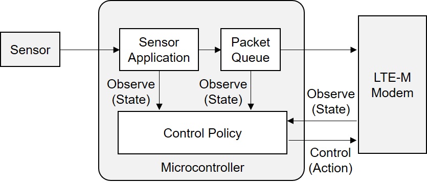
Figure 2: Block diagram of wireless sensor CPS.

Due to the LTE-M power profile, a feasible use case for a system like this would be to keep the modem powered off by default, periodically turn it on to exchange data with the Internet and then power it back down to conserve energy. To model this use case, we controlled our Sequans Monarch LTE-M modem from a test application on a laptop computer that powered the modem on, connected to the nearest Verizon Wireless cell tower, transmitted some information (representing a sensor reading) from the test application to a cloud-based server, then disconnected the cell tower connection, and finally powered down the modem. During multiple runs of this test, we measured the power consumption of the LTE-M modem. A typical current versus time trace of the energy required by the modem to perform this procedure is shown in Figure 3. The trace is a time-series of current draw in milli-Amperes at a fixed voltage of 4.0 Volts, and thus instantaneous power and total energy for the transaction can both be computed from the data.

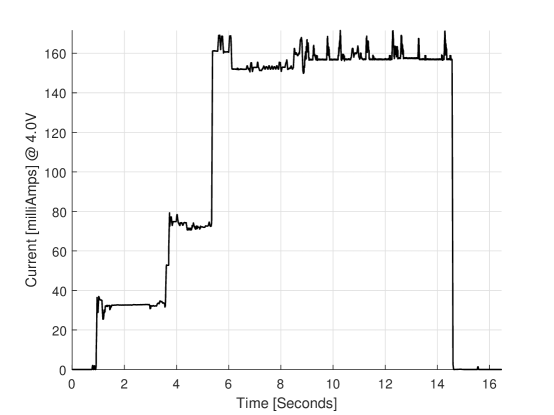
Figure 3: Current consumption of LTE-M modem during data transfer.

Additionally, we varied the quantity of data that we transmitted to the server on each test run. Specifically, we used a packet size of 256 Bytes per packet and varied how many of these fixed-sized packets were transmitted. These measurements helped us quantify the approximate energy consumption of the LTE-M modem as a function of the amount of data transmitted. This allowed us to create an approximate model of the modem power consumption, as a function of the quantity of packets transmitted. Our derived model is given by Equation 6:

$$\begin{split}E_{TX}(N_{T})=c_{1}+c_{2}({N_{T}}-1)\,[\mathit{Joules}]\\ {N_{T}}\geq 1,c_{1}=6.62,c_{2}=1.55,\end{split}$$ (6)

where $E_{TX}$ is the energy consumption in Joules and $N_{T}$ is the number of packets. This equation illustrates a defining characteristic of this type of wireless connection: the energy overhead of powering the modem on and connecting to a cell tower can be significantly higher than the incremental cost of transmitting a packet once the connection is active. Thus, if optimizing strictly for energy efficiency it is advantageous to queue up multiple packets before powering on the modem, and then transmit the queued packets together. This approach, however, is the opposite of what should be done if optimizing for transmission latency. This is a fundamental trade-off of controlling the LTE-M modem in this CPS node.

The power control challenge for a system like this consists of implementing an algorithm that strategically determines when to allow new sensor data to accumulate in the sensor, versus when to invoke a communication event (which would produce a power consumption profile similar to the one shown in Figure 3) that transfers all packets in the queue up to the cloud-based server. This decision problem involves a trade-off of energy efficiency versus communication latency.

A trivially simple policy is one where any time a new packet arrives in the queue, it is immediately transmitted up to the cloud. In fact, this could be considered a default case where no control policy analysis had occurred, and the MCU program was designed simply to transmit whenever a new packet exists. However, this is still a control policy and we consider it as such. This policy will have a low energy efficiency (which is undesirable) and low communication latency (which is desirable).

In another example, a controller could wait until a fixed number of packets accumulate in the queue before doing a batch transfer of all accumulated packets up to the cloud. This policy would have higher energy efficiency but also higher communications latency, as some packets might sit in the queue for some time before being sent to the server. Ultimately, the CPS node’s application will dictate what type of latency is desirable for the system, and it should be made as efficient as possible while meeting the specified latency goals.

The policies described above are both very simple “fixed threshold” policies. These are easy to implement and analyze for the dynamics described thus far. However, in a real-world CPS deployment, the system control dynamics are likely to be more complicated and time-varying than has been described so far. Additional complexity arises from the following phenomena:

• The application is likely to be multi-modal and thus the rate of packet generation within the CPS node is in general time-varying.

• The number of different modes that the application may contain could be much more than two.

• The modem connection time and power consumption are also time-varying due to the physical mobility of the CPS node relative to the fixed location of the cell tower as well as the presence of network congestion from other LTE-M users within the same cell during periods of heavy usage.

When these real-world factors are modeled, it becomes advantageous to consider more involved control policies that can monitor and adapt to the time-varying conditions which may not be precisely modeled prior to a system deployment. For this reason, we consider two approaches that contain online learning capabilities specifically to self-optimize continuously at runtime, adapting to the time-varying nature of the CPS node’s environment. This feature avoids having to understand and anticipate all of the runtime conditions ahead of time, which for practical purposes is an infeasible requirement for real-world deployments that have high numbers of nodes.

In Sections 6 through 8, we first describe multiple options for controlling the CPS node in our case study and then compare the performance of the policies with regard to the efficiency versus latency trade-off in simulation. Afterwards, we implement the competing options on a resource constrained MCU and detail the resulting computational requirements and deployment feasibility.

6 MDP-Based Control

In this section we detail two approaches to create control policies for the CPS node introduced in Section 5, and then compare their performance using simulation. Both approaches use discrete-time MDPs to generate a control policy, which determines when to power the LTE-M modem on and off. The controllers are both designed with the assumption that several of the system’s characteristics and dynamics are time-varying and uncontrollable. Thus, both controllers employ some form of learning, in that the policy that each controller employs is continually updated to reflect the time-varying changes in both the system it is controlling and the environment that the system interacts with at any given time. The two controllers can be viewed as being two different realizations of the agent component in the framework of Figure 1. We refer to the two methods as: 1) the Structured Learning controller and 2) the Q-Learning controller. The Structured Learning controller is a novel approach described for the first time in this paper, and the Q-Learning controller is a well known technique in the RL literature (e.g. [1]).

Table 1: Comparison of two MDP-based controllers.

	Structured Learning	Q-Learning
State Space	Common$\colon\mathcal{S}$
Action Space	Common$\colon\mathcal{A}$
Rewards	Common$\colon R(s,a)$
STM	Explicitly defined, parameterized	Not needed
Policy Generation	Solver invoked at runtime	Temporal difference equation used to estimate Q function

A summary of the differences between the controllers is shown in Table 1. The MDP components that are common between the two controllers are: the discrete state space $\mathcal{S}$, the discrete action space $\mathcal{A}$, and the reward function $R(s,a)$. The other components of the controllers are different, namely the STM and policy generation method. The Structured Learning controller contains a parameterized state transition matrix and employs an MDP solver at runtime to generate a control policy. In contrast, the Q-Learning controller does not contain an explicit state transition matrix, and instead contains a running estimate of the MDP’s Q function. This allows the Q-Learning controller to completely bypass having to store an STM and run an MDP solver.

One fundamental difference between the two techniques is that the Structured Learning controller has an STM with a pre-populated structure, and only parameters within the structure need to be learned at runtime. There are some aspects of the STM that are fixed at design time, and in this way, some structure does not need to be learned. In contrast, the Q-Learning controller has no a priori structural assumptions, and must learn the entire Q function at runtime. Depending on how much of the STM is known at design time in a given application, the Q-Learning controller may have to learn more parameters at runtime compared to the Structured Learning controller.

Table 2: Number of parameters to learn at runtime for each controller.

Structured
Learning	Q-Learning
$0\leq\left|{\Theta}\right|\leq{({N_{S}}-1){N_{S}}{N_{A}}}$	${N_{S}}{N_{A}}$

This contrast is shown in Table 2, where $\Theta$ is the number of unknown or time varying parameters in the STM, as was defined in Equation 2. This motivates a general design guideline to be considered: to determine what type of learning approach to use, an engineer should first analyze the percentage of the STM that is known versus the percentage that is unknown or expected to be time-varying. In other words, the designer should seek to minimize the number of parameters that need to be learned at runtime, which is $\left|{\Theta}\right|$ in Structured Learning, and ${N_{S}}{N_{A}}$ in Q-Learning (recall that $\left|{\Sigma}\right|$ denotes the cardinality of a set $\Sigma$). If many parameters out of the STM need to be learned at runtime, it is possible that $\left|{\Theta}\right|\geq{N_{S}}{N_{A}}$, in which case the Q-Learning approach would have less parameters to learn at runtime and likely provide better adaptation performance.

The two different controller designs investigated in this section were formulated to concretely explore trade-offs between model-based (Structured Learning) and model-free (Q-Learning) in a tangible, real-world example. In the remainder of this Section we first detail the common components of the two techniques, and then elaborate on their differences.

6.1 State and Action Spaces

Both controllers utilize a multivariate state space, a concept introduced in Section 3.1. The MDP state space is essentially the combination of each of the states of the sensor application, packet queue and LTE-M modem. This is defined as shown in Equation 7:

$$\begin{split}s=(s_{a},s_{q},s_{m})\in\mathcal{S}\\ s_{a}\in\{0,1,..,N_{SA}-1\},\\ s_{q}\in\{0,1,...,N_{SQ}-1\},\\ s_{m}\in\{0,1,..,N_{SM}-1\},\end{split}$$ (7)

where $s\in\mathcal{S}$ is the state variable, which is composed of there separate variables $s_{a},s_{q},s_{m}$: the sensor application state, queue state and modem state, respectively.

In general, we are interested in applications that can run in one of a set of alternative modes (see Section 5). Thus we define $s_{a}$ as the application mode, a state variable taking a value out of a discrete set of $N_{SA}$ modes. The packet queue has a specific number of packets in it at any given time. In order to allow the controllers to make decisions based on the current state of the queue, we define $s_{q}$ as the number of packets in the queue and make it part of the MDP state space.

We assume that the queue is of a fixed size $N_{SQ}-1$, due to our goal of housing it in a resource constrained MCU. The queue can only hold up to $N_{SQ}-1$ packets, and any attempts to queue additional packets beyond this limit will result in the newest packet being discarded. The discarding of a packet represents a loss of data and is a very undesirable event, that our controllers must seek to avoid through the decisions in their respective control policies.

Note that in other applications, some amount of data loss may be tolerable. Such applications can be accommodated readily in both controller designs by making suitable adaptations. We omit details of these adaptations in this paper for brevity.

The LTE-M modem is a complex mixed-signal System-On-Chip (SoC), containing the LTE-M protocol implementation and runtime signal processing. There is an enormous state space that could be defined for the inner workings of the modem. However, for our controllers the majority of that information is not relevant and thus we collapse the modem state into a small set of states that is detailed enough for the controller to implement a high performing control policy, without being overly burdened with the computational and storage implications of a large state space. In this spirit, we leverage the concept of Transition States introduced in Section 3.4, and collapse the large number of fine-grained LTE-M modem states into three coarse-grained states: ${M\_OFF}$, ${M\_CONNECTING}$, and ${M\_CONNECTED}$. The ${M\_CONNECTING}$ state is a transition state, and the other two are not.

${M\_OFF}$ refers to the modem being fully powered off, and the modem can remain in this state indefinitely until commanded otherwise. ${M\_CONNECTING}$ is the state that begins immediately after the modem has been powered on and ends when a successful Internet connection has been established. The modem cannot remain indefinitely in this state. By definition, it is guaranteed to transition out of this state after a specified amount of time steps. ${M\_CONNECTED}$ is the state when a working Internet connection has been established and continues to be maintained. Transmission of packets is only possible in the ${M\_CONNECTED}$ state. This modeling approach forces us to pick a scalar constant for the modem’s power consumption in each of the three states.

As can be observed from Figure 3, the power is roughly constant in the ${M\_OFF}$ and ${M\_CONNECTED}$ states. However, this is not the case in the ${M\_CONNECTING}$ state. We address this by representing power consumption during the entire transition as a fixed value: the average power consumption during the duration of the transition. This simplification is a way of providing the MDP the information that it needs to implement a high performing policy, in as compact a representation as possible. This modeling approach is a design choice, and we note that an interesting area for future study is in the trade-offs for varying levels of modeling expressiveness in this area.

In this system, the controllers are being tasked with turning the LTE-M modem on and off. This binary control implies an “on” action that powers on the LTE-M modem and commands it via the modem’s interface to attach to the cell tower and establish an Internet connection. Conversely the “off” action implies tearing down any existing Internet connections, and shutting off the LTE-M modem gracefully via the modem’s shutdown procedures. The resulting action space is shown in Equation 8. The two actions $\mathit{off}$ and $\mathit{on}$ in Equation 8 are abstractions of multi-step LTE-M modem command sequences.

$$a\in\mathcal{A}=\{\mathit{off},\mathit{on}\}$$ (8)

6.2 Rewards

In order to “motivate” the controllers to find an effective balance to the latency versus energy efficiency trade-off described in Section 5, we define the reward function as shown in Equation 9. The reward function maps each state-action pair $(s,a)$ to a scalar reward.

$$\begin{split}R(s,a)=r_{1}I(s,a)+r_{2}N_{T}(s,a)+r_{3}N_{D}(s,a),\\ r_{1}=-10,\\ r_{2}\in\{3,4,...,10,100,1000\},\\ r_{3}=-100,\end{split}$$ (9)

where $I(s,a)$ is the average electrical current consumed by the modem, $N_{T}(s,a)$ is the number of packets known to be transmitted, and $N_{D}(s,a)$ is the number of packets dropped by the modem due to an overflowing queue in the previous timestep. For each of these quantities we use the function arguments $(s,a)$ to denote the respective value of each of the terms known, expected, or averaged when action $a$ is taken in state $s$. Instead of power consumption, we use electrical current in its place due to it being equally suitable (given a constant voltage) and more straightforward to measure with an MCU in an embedded system.

With this formulation, the scalar reward is thus a linear combination of observable time-varying signals and quantities. This formulation steers both controllers to our desired goals, by rewarding them (with a positive reward value) when a packet is transmitted successfully and penalizing them (with a negative reward value) when electrical current is consumed or the packet queue overflows. The reward constants $r_{1},r_{3}$ were selected via experimentation and $r_{2}$ was left as a free parameter in order to be able to generate a set of instances for each controller. Each instance in the set places different amounts of importance on the latency requirement relative to the energy efficiency requirement. This approach allowed us to simulate a suite of controllers for each method, and plot the resulting performance for a more robust comparison. The resulting policies are ones where the respective controllers turn the modem on and off at each discrete time step, in the way they determine is the optimal approach for obtaining the maximal rewards. In other words, they attempt to transmit the packets generated by the sensor application without incurring undesired delay or consuming more electrical power than is needed, through dynamic and changing conditions.

In Section 6.3 through Section 6.4, we detail the differences between the two controllers that we are evaluating in this case study.

6.3 Structured Learning Controller

The Structured Learning controller consists of the common components described above, plus the addition of the STMs and an MDP solver. The STMs are described in this section, and the solver is described in Section 8.

The stored STMs at any given time are a combination of constants and time-varying parameter estimates. The constants are programmed in at design time, and the estimates are maintained by observing samples of the relevant quantities, and using the Temporal Difference (Equations 3) method to update the estimates. The estimates are plugged into the STM data structures, which serve to maintain fully populated STMs at each time step.

The STMs are constructed using a factored formulation, which greatly reduces the storage requirements of the MDP. The factorization procedure is shown in Equation 10 through Equation 14. The factorization serves to convert one large multivariate conditional probability distribution into a product of terms functions, each having the form of a lower dimensional conditional probability distribution. The terms correspond to the subsystems of the sensor application, packet queue and LTE-M modem, respectively. This re-arrangement causes a significant reduction on the MDP storage requirements.

$$p(s^{(n+1)}|s^{(n)},a^{(n)})=p(s_{a}^{(n+1)},s_{q}^{(n+1)},s_{m}^{(n+1)}|s^{(n)},a^{(n)})$$ (10)

$$=p(s_{a}^{(n+1)}|s_{q}^{(n+1)},s_{m}^{(n+1)},s^{(n)},a^{(n)})\cdot p(s_{q}^{(n+1)},s_{m}^{(n+1)}|s^{(n)},a^{(n)})$$ (11)

$$=p(s_{a}^{(n+1)}|s_{a}^{(n)})\cdot p(s_{q}^{(n+1)},s_{m}^{(n+1)}|s^{(n)},a^{(n)})$$ (12)

$$=p(s_{a}^{(n+1)}|s_{a}^{(n)})\cdot p(s_{q}^{(n+1)}|s_{m}^{(n+1)},s^{(n)},a^{(n)})\cdot p(s_{m}^{(n+1)}|s^{(n)},a^{(n)})$$ (13)

$$=p(s_{a}^{(n+1)}|s_{a}^{(n)})\cdot{}p(s_{q}^{(n+1)}|s^{(n)},a^{(n)})\cdot{}p(s_{m}^{(n+1)}|s_{m}^{(n)},a^{(n)})$$ (14)

6.3.1 Sensing Application

Given the observability of the sensing application’s mode, the controller can maintain parameters that statistically characterize how often the application is in a given mode, and how likely the CPS is to transition from any mode to any other given mode. These characterization parameters are listed in Equation 15. Using the latest values of these parameters, the $s_{a}$ term of the factored STM can be fully instantiated.

$$\begin{split}\hat{\sigma}_{i,j}=p(s_{a}^{(n+1)}=j|s_{a}^{(n)}=i)\forall(i,j)\in\{0,1,...,N_{SA}-1\}^{2}\\ \end{split}$$ (15)

6.3.2 Packet Queue

Since it is part of the state space, the dynamics of the queue must also be modeled as a transition matrix. This results in having to model a fully deterministic process into stochastic structures in order to fit into the MDP framework, and thus most of the probabilities are either 1 or 0. The transition probabilities are almost all known at design time, since the dynamics of the queue do not change. The only uncertainty comes from the rate of packets entering the queue from the sensing application, and the rate leaving the queue from the LTE-M modem connection.

The packet queue’s state is defined as the number of packets in it at a specific timestep. The transition probabilities amount to the likelihood of transition to another state, in other words the change in the number of packets. The transition to a state where more packets are inserted corresponds directly to the sensing application’s packet generation rate. These events are combined with the probability of packets being removed from the queue by being transmitted to the cloud server. If the modem state and action are such that the modem is not yet connected, then no packets can leave the queue and thus transitions to states where the number of packets is reduced are not possible. If the modem is connected, then packets can leave the queue.

6.3.3 LTE-M Modem

In our model, the dynamics of the LTE-M modem are a direct application of the Transition State concept. In order to instantiate this component of the STM, the controller needs to maintain a running estimate of how long the LTE-M modem takes to connect to the network. We refer to this time-varying quantity as $T_{C}$ and its most recent estimate as $\hat{T}_{C}$. With this estimate, the resulting transition probabilities are shown in Figure 4. Following the Transition States theory from the literature (e.g.  [15]), the value of the parameter $\rho$ is defined in Equation 16, where $T_{F}$ is the duration of one control frame.

As can be observed from the Figure 4 and Equation 16, this component of the STMs is parameterized by the running estimate $\hat{T}_{C}$ (through $\rho$) in two elements, and combined with known constants for the remaining elements.

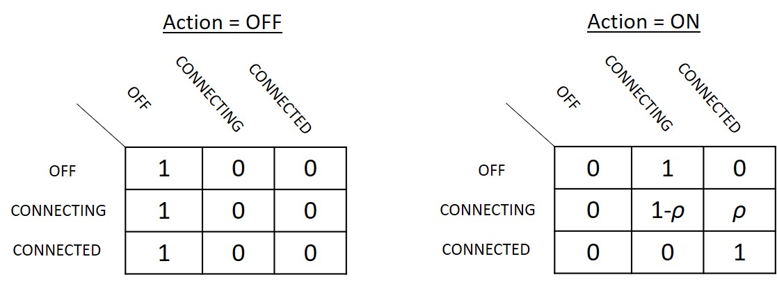
Figure 4: State transition matrices for LTE-M Modem.
Only the parameter $\rho$ is learned at runtime.
The remaining entries are specified at design time.

$$\hat{\rho}=\left[\mathit{floor}\left(\frac{\hat{T}_{C}}{T_{F}}\right)\right]^{-1}$$ (16)

6.4 Q-Learning Controller

The Q-Learning controller was implemented directly from the description of the technique in [1]. In this method, a function $Q$ is created as a mapping $Q(s,a):(S\times A)\rightarrow\mathbb{R}$, where $\mathbb{R}$ denotes the set of real numbers. Each mapping in the function represents an estimate of the total amount of reward an agent can expect to accumulate over the future, starting from a given state $s$ and taking a given action $a$. The $Q$ function is updated on each iteration of the controller using the Temporal Difference. Using the latest estimated version of $Q(s,a)$, the action is selected by comparing all actions for the given state $s$ and selecting the action with the largest value. The remaining details of the Q-Learning method can be found in [1].

7 Simulation

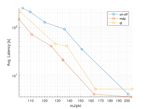
Figure 5: Simulation Results: Energy efficiency versus communication latency.

In order to objectively compare the runtime performance of the Structured Learning and Q-Learning controllers presented in Section 6, we created a MATLAB simulation containing models of all the subsystems described in the case study. In our simulation testbed, a sensor application generates packets at rates consistent with a given mode, and also simulates the transition between modes at specified transition rates. A packet queue object models a generic fixed length queue, which acts as a First In First Out (FIFO) data structure, and overflows if the maximum number of elements is exceeded. A stochastic model of the LTE-M modem was created using the collected time-series data and electrical power measurements (see Section 5.1).

The simulation was run with three separate controllers: the two MDP-based controllers described in the previous section, as well as a third manually-generated policy. The manually-generated policy simply checks the queue, and turns on the modem any time a specified number $N_{q}$ of packets are in the queue, where $N_{q}$ is a parameter of the policy. Once the modem is turned on, it remains on until the queue is fully drained.

The simulation was run multiple times for each controller, and each simulation run is represented by a single point in the graph of Figure 5. The fixed threshold (manually generated), Structured Learning, and Q-Learning approaches are denoted by the “onoff”, “mdp”, and “ql” traces, respectively. The best performance corresponds to points that have the lowest average communication latency (the vertical axis) and simultaneously the lowest average energy efficiency (the horizontal axis).

For the fixed threshold technique, we generated multiple policies by varying the $N_{q}$ threshold at which the modem was powered on. For the MDP-based controllers, we varied the $r_{2}$ constant in the reward function from Equation 9. This approach gave us a set of control policies for each controller, allowing us to fully explore the performance limits of each technique.

Our first conclusion from the data in Figure 5 is that both MDP-based controllers outperform the fixed threshold approach, for all possible values of the $N_{q}$ threshold. We believe this to be due to richer and more expressive policies generated by the MDPs; while the fixed threshold policies are a function of the packet queue state only (ignoring the application and modem characteristics), the MDP-based policies materialized as a function of the entire state space. In this case study, since the MDP is able to reason using algorithmic methods on data structures and computations on conditional probabilities, it can consider more effects and consequences systematically and produce highly optimized policies that are more expressive relative to the simple, manually-derived, fixed threshold heuristic.

Our second conclusion from the data is that the Structured Learning controller outperforms the Q-Learning controller. As an example, if we tune the rewards such that both learning controllers achieve an average packet transmission latency of 20 seconds, the Structured Learning controller is able to accomplish this with an average energy efficiency of 135 mJ per packet, compared to 163 mJ per packet on the Q-Learning controller. This amounts to a 17% savings in the transmission energy for sending the exact same packets at the same average latency. This can be an important difference since transmission energy is often the largest source of energy consumption on an LTE-M connected sensor.

We believe that Structured Learning outperforms Q-Learning in this example because we have focused its learning on only the time-varying aspects of the system (e.g. modem power, cell tower connection time, etc.) and have designed it to accept as unquestionable truth the other dynamics and attributes (e.g., that the packet queue contains one less packet after a packet is removed from it, etc.). In contrast, the Q-Learning controller is forced to learn (and continue to update indefinitely) all aspects of the system transition probabilities in response to selected actions. It must continually experiment with exploratory actions and accumulate data to learn all of the system dynamics (including well understood behavior, such as the packet queue’s dynamics), and our results demonstrate that expending learning effort on such immutable aspects is both unnecessary and detrimental to the overall system performance.

8 Implementation

In this section, we detail the results of implementation experiments performed to assess the viability of the competing MDP-based control strategies in the context of a state-of-the-art processing platform for resource-constrained CPSs. The alternatives are implemented on a typical MCU that would be used to realize our CPS case study, and are compared in terms of their execution time, memory usage and processing power consumption.

8.1 Experimental Setup

The competing controllers were implemented on the Silicon Labs EFM32GG, a small and low power ARM Cortex M3-based MCU. The processor was running on the EFM32 STK3700 development kit, which houses the CPU as well as sophisticated energy monitoring circuitry. The EFM32GG contains 128 kB of RAM and 1MB of FLASH, which make it a reasonably capable platform for the CPS in our case study at the time of this writing.

In order to compare the controllers objectively, we created the following experimental setup on the EFM32GG development board. All controllers were implemented in C and stored in the MCU’s program memory one at a time. Memory usage was computed by statically allocating all data structures and examining the map file that the MCU’s compiler generates. A common test harness was written for the EFM32GG, which was driven by a periodic timer interrupt. The interrupt rate was configured to be 100ms, which we use as the fixed-period discrete-time iteration rate for the controllers.

The C program initially puts the CPU into its low power sleep mode. It remains in that mode until the periodic interrupt fires. Once the interrupt fires, the MCU is woken from sleep and it then executes the computations needed for one iteration of the controller under test. Once the iteration has completed, the MCU returns back to sleep mode where it waits for the next firing of the periodic interrupt. Since the sleep current is extremely low compared to the run current (microAmps compared to milliAmps), this approach allowed us to precisely measure both the execution time and computational energy required to execute each controller on the MCU by observing the current versus time profile of each controller. Real-time MCU current consumption was measured by using the EFM32GG board’s energy monitoring tools, which allow very accurate current versus time data to be observed in the form of a high resolution time-series waveform capture.

Using this simple fixed rate scheduling scheme combined with the Cortex-M3 sleep modes and the development board’s current monitoring tools, we were able to observe the execution time and processing current consumed by the CPU for each control policy. This testbench provided a highly repeatable experimental setup where all settings were kept the same from case to case with the only difference being the control policy being used.

8.2 Matrix Format

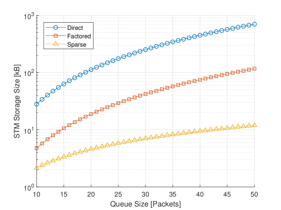
Figure 6: Transition matrix storage sizes.

In our case study’s MDP, the number of states $N_{S}$ is 66, and the number of actions $N_{A}$ is 2. The number of non-zero elements $K_{NZ}$ in the STMs is 444. This represents a sparsity of 94.9%. Aside from the direct implementation of the full STMs, we evaluated two CMM techniques: a factored implementation and a sparse implementation. In Figure 6, we show the resulting STM storage sizes for these techniques on our case study, over a range of packet queue sizes.

As can be observed from the data, both the factored and sparse implementations reduce storage size considerably. However, the sparse method is the most effective in this regard and for this reason we selected this approach for the implementation.

8.3 Measurements

8.3.1 Memory Usage

Table 3: Data storage size in kiloBytes.

	Structured	Sparse Structured
	Learning (VI)	Learning (SVI)	Q-Learning
$\mathit{STM}$	34.0 kB	2.60 kB	-
Rewards	0.51 kB	0.51 kB	0.51 kB
Q-Function	-	-	528 B
Total	34.5 kB	3.11 kB	1.03 kB

First, we compared the techniques in terms of how much data storage each required on the MCU. The results are shown in Table 3, where the column labeled Sparse Structured Learning represents the Structured Learning method implemented with sparse matrices, as described in Section 4.3.

We observe from Table 3 that the Q-Learning approach is the most favorable in this metric, and furthermore show that it requires significantly less data storage than the Structured Learning (VI) approach. However, when we apply the SVI method to Structured Learning, we see a huge reduction in the required data storage compared to VI. We conclude that in this case study, the CMM techniques reduce the storage requirements of Structured Learning to be much closer to that of Q-Learning, while not beating it in this regard.

Generalizing these results beyond the case study, it can be seen from Table 3 that all of the methods being compared require the same amount of storage for the reward function. Thus, the difference in memory usage is attributed to the storage of the STMs in the VI and SVI controllers, compared to only the Q-Function in the Q-Learning controller. This difference can be calculated in the general case as follows. Assuming STM entries are 4 byte single precision floating point values, the Q-Function can be stored in $4{N_{S}}{N_{A}}$ bytes, as it consists of a table of ${N_{S}}{N_{A}}$ floating point values. The storage size of the STMs in the Structured Learning (VI) method is $4{{N_{S}}^{2}}{N_{A}}$ bytes, as it consists of $N_{A}$ stochastic matrices, each of size $({N_{S}}\times{N_{S}})$.

The STMs in the Sparse Structured Learning (SVI) method were implemented with sparse matrices stored in coordinate format [32]. This format stores only the non-zero elements of a matrix, along with two indices representing the column and row index of the element, respectively. Assuming that $\lceil{\mathit{log}_{2}(N)/8}\rceil$ bytes are required to store an integer index that can take on one of $N$ values, the storage size required for the STMs in coordinate format is shown in Equation 17, where $K_{\mathit{NZ}}$ is the number of non-zero elements in the STMs.

$$K_{\mathit{NZ}}(\lceil{\mathit{log}_{2}(NsNa)/8}\rceil+\lceil{\mathit{log}_{2}(Ns)/8}\rceil+4)$$ (17)

Evaluating the formula above (Equation 17) using the constants from the case study ($N_{S}=66$, $N_{A}=2$, $K_{\mathit{NZ}}=444$) results in the storage sizes shown in Table 3. The formula can be used to predict the required storage sizes for other case studies by appropriately changing the values of ($N_{S},N_{A},K_{\mathit{NZ}}$).

8.3.2 Computation

Table 4: Execution time (in seconds), computation energy (in Joules)
and average power (in Watts).

	Structured	Sparse Structured
	Learning (VI)	Learning (SVI)	Q-Learning
Per Control Iteration:	3.5 $\mu$s / 117 nJ	3.5 $\mu$s / 117 nJ	211 $\mu$s / 7.06 $\mu$J
Per Solver Iteration:	50.1 s / 1.67 J	5.61 s / 187 mJ	-
Average Power	483 $\mu$W	69.8 $\mu$W	78.8 $\mu$W

Next, we measured the execution time and power consumption of the MCU when executing the control algorithms for each of the competing techniques. We observe that Q-Learning requires the same computation on every control period. This consists of updating the Q-Function based on the observed state transition and reward, and computing the best action for a given state using the latest values in the Q-Function. The Q-Learning method performs these operations on every control period.

In contrast, the Structured Learning techniques (VI and SVI) run a solver, which we invoked once per hour. These techniques compute a new control policy every hour, and the time and energy required to do this is shown in the second row of Table 4. After computing a new policy every hour, the Structured Learning techniques simply look up which action to use from a stored table for the remainder of that hour.

From Table 4, we see that the Structured Learning techniques (represented in the second and third columns of data) involve much less computation time and energy consumption during a typical control period relative to Q-Learning. Note that the first row of data for Structured Learning in Table 4 excludes the computation associated with solver execution, while the third row of data (labeled Average Power) includes the effects of solver computation.

We note that the Structured Learning implementation would likely require a priority-based pre-emptive scheduling scheme such that the control iteration execution would take higher execution priority over the solver, such that any real-time deadlines associated with the controller are not missed due to running the solver.

We conclude from the data in Table 4 that although Q-Learning does consume less average power (third row of data) than Structured Learning (VI), when we apply the SVI method to Structured Learning we achieve less average power compared to Q-Learning. SVI reduces computation time by replacing standard matrix operations by sparse matrix operations. This results in a significant reduction in computation time, given that the STMs are extremely sparse.

Generalizing these results beyond the case study, we identify the factors that affect which of the methods is favorable in terms of computation costs — e.g., processing time and energy consumption. In the Structured Learning techniques, the size of the MDP and complexity of the STMs determine how long it takes to execute a solver to produce a control policy. If the MDP is very large and complex, the solver will take longer to execute. In contrast, the Q-Learning technique is not affected at all by this attribute. In this aspect, it can be concluded that Q-Learning is better suited to deal with large MDPs than Structured Learning in terms of computation expense.

Another factor that is relevant is how often the Structured Learning techniques are required to compute an updated policy. In general, a suitable update rate is determined by the application’s adaptation requirements, and how quickly the time varying environment is changing. In the case study presented here, the policy is updated once per hour, but a system that adapts to more slowly changing dynamics may only need to update the control policy once per day or even less frequently. On the other hand, a system adapting to fast changing dynamics may need to update the policy much more often, such as once per second. A faster update rate will generally increase the computational cost of the Structured Learning techniques, whereas Q-Learning is not affected by this consideration at all. In this regard, Structured Learning is better suited to applications were the adaptation is on dynamics that are varying relatively slowly in time.

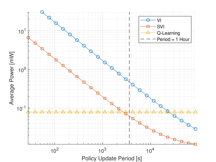
Figure 7: Average power consumed by the MCU on competing control algorithms
as a function of the policy update period.

In this case study, the data point of a 1 hour update period leads to Sparse Structured Learning having lower computational cost than Q-Learning. The crossover point where Q-Learning consumes less computational power is shown in Figure 7 to be approximately at 45 minutes. It is important to note that this crossover point is specific to the MDP size and complexity (affecting solver execution time) and the choice of MCU (affecting run current, sleep current, and solver execution time).

In summary, from the results of this and the preceding section, we see that Structured Learning with SVI is capable of applying control policies that are more robust compared to Q-Learning at a slightly lower average computational power consumption. Although the memory requirement overhead of SVI is greatly reduced compared to VI through the exploitation of sparsity, it is still slightly larger than that of Q-Learning.

9 Conclusion

In this work, we have provided a survey of recent developments in Compact MDP Models (CMMs), and by integrating several complementary CMM techniques, we have presented a novel CMM-based approach to CPS design. We have provided comparisons between CMM-based methods and Q-Learning in the context of CPS. The differences between the two approaches were explored conceptually, as well as through a detailed case study involving both simulation and a prototype implementation.

From the results of this work, we conclude that Q-Learning can be considered a more robust technique when either very little is known about the system a priori, or a large percentage of the dynamics are expected to continually change at runtime. In contrast, when a significant portion of the system’s environment or its dynamics are predictable, the CMM option can provide a substantially more efficient and robust approach.

An LTE-M connected sensor was detailed as a CPS case study to compare a CMM-based learning controller to an alternative controller that used Q-Learning. For a specified average packet transmission latency, the CMM-based controller resulted in a 17% reduction in LTE-M transmission energy, which is often the largest source of energy consumption on an LTE-M connected sensor. The energy savings are accomplished through strategic management of the LTE-M modem and connection status, using learned dynamics of the system and its environment.

Since the learning controller must be implemented in the deployed system, and its processing can be considered an overhead to the LTE-M connected sensor’s main purpose, we also analyzed the implementation costs of the two learning controllers. The implementation was on a small microcontroller that is typical of what would be used for such a CPS system. In this experiment, it was found that the CMM-based controller used 69.8 $\mu$W compared to 78.8 $\mu$W for the Q-Learning controller, an 11.4% savings. However, the CMM-based controller required more RAM to store its data structures — 3.11kB compared to 1.03kB.

Useful directions for future work include explorations into other challenging CPS case studies with larger state spaces, and continued development of compact techniques that provide self-awareness and runtime adaptation capabilities at all levels of embedded implementation.

10 Acknowledgements

This research was sponsored in part by the US National Science Foundation (CNS1514425 and CNS151304).

References

- [1] R. Sutton and A. Barto, Reinforcement Learning: an Introduction, 1st ed. MIT Press, 1998.
- [2] A. Sapio, S. Bhattacharyya, and M. Wolf, “Efficient solving of Markov decision processes on GPUs using parallelized sparse matrices,” in Proceedings of the Conference on Design and Architectures for Signal and Image Processing (DASIP), Oct 2018.
- [3] L. Benini, A. Bogliolo, and G. D. Micheli, “A survey of design techniques for system-level dynamic power management,” IEEE Transactions on Very Large Scale Integration (VLSI) Systems, June 2000.
- [4] A. Kansal, J. Hsu, S. Zahedi, and M. B. Srivastava, “Power management in energy harvesting sensor networks,” ACM Transactions on Embedded Computing Systems, vol. 6, no. 4, 2007.
- [5] Q. Liu et al., “Power-adaptive computing system design for solar-energy-powered embedded systems,” IEEE Transactions on Very Large Scale Integration (VLSI) Systems, vol. 23, no. 8, pp. 1402–1414, 2015.
- [6] C. Hsieh, F. Samie, M. S. Srouji, M. Wang, Z. Wang, and J. Henkel, “Hardware/software co-design for a wireless sensor network platform,” in Proceedings of the International Conference on Hardware/Software Codesign and System Synthesis, 2014, pp. 1–10.
- [7] C. Moser, L. Thiele, D. Brunelli, and L. Benini, “Adaptive power management in energy harvesting systems,” in Proceedings of the Design, Automation and Test in Europe Conference and Exhibition, 2007, pp. 1–6.
- [8] C. Moser, L. Thiele, D. Brunelli and L. Benini, “Adaptive power management for environmentally powered systems,” IEEE Transactions on Computers, vol. 59, no. 4, pp. 478–491, April 2010.
- [9] L. Esterle and B. Rinner, “An architecture for self -aware IoT applications,” in 2018 IEEE International Conference on Acoustics, Speech and Signal Processing (ICASSP), April 2018, pp. 6588–6592.
- [10] N. Dutt, A. Jantsch, and S. Sarma, “Toward smart embedded systems: A self-aware system-on-chip perspective,” ACM Trans. Embed. Comput. Syst., vol. 15, no. 2, pp. 22:1–22:27, Feb. 2016.
- [11] P. R. Lewis, M. Platzner, B. Rinner, J. Torresen, and X. Yao, Self-aware Computing Systems: An Engineering Approach. Springer, 2016.
- [12] L. Benini, A. Bogliolo, G. A. Paleologo, and G. De Micheli, “Policy optimization for dynamic power management,” IEEE Transactions on Computer-Aided Design of Integrated Circuits and Systems, vol. 18, no. 6, pp. 742–760, June 1999.
- [13] Y. Wei, X. Wang, F. Guo, G. Hogan, and M. Collier, “Energy saving local control policy for green reconfigurable routers,” in IEEE International Conference on Communications, 2015, pp. 221–225.
- [14] A. Sapio, M. Wolf, and S. S. Bhattacharyya, “Compact modeling and management of reconfiguration in digital channelizer implementation,” in Proceedings of the IEEE Global Conference on Signal and Information Processing, Washington, D.C., December 2016, pp. 595–599.
- [15] A. Sapio, L. Li, J. Wu, M. Wolf, and S. S. Bhattacharyya, “Reconfigurable digital channelizer design using factored Markov decision processes,” Journal of Signal Processing Systems, December 2017. [Online]. Available: https://doi.org/10.1007/s11265-017-1319-6
- [16] Y. Debizet, G. Lallement, F. Abouzeid, P. Roche, and J. Autran, “Q-learning-based adaptive power management for iot system-on-chips with embedded power states,” in Proceedings of the IEEE International Symposium on Circuits and Systems (ISCAS), May 2018, pp. 1–5.
- [17] E. Jung, F. Maker, T. L. Cheung, X. Liu, and V. Akella, “Markov decision process (MDP) framework for software power optimization using call profiles on mobile phones,” Journal of Design Automation for Embedded Systems, vol. 14, no. 2, pp. 131–159, 2010.
- [18] S. Russell and P. Norvig, Artificial Intelligence: A Modern Approach, 3rd ed. Pearson, 2009.
- [19] O. Sigaud and O. Buffet, Eds., Markov Decision Processes in Artificial Intelligence. Wiley, 2010.
- [20] A. D. Tijsma, M. M. Drugan, and M. A. Wiering, “Comparing exploration strategies for Q-Learning in random stochastic mazes,” in Proceedings of the IEEE Symposium Series on Computational Intelligence (SSCI), Dec 2016, pp. 1–8.
- [21] R. C. Hsu, C. T. Liu, and H. L. Wang, “A reinforcement learning-based ToD provisioning dynamic power management for sustainable operation of energy harvesting wireless sensor node,” IEEE Transactions on Emerging Topics in Computing, vol. 2, no. 2, pp. 181–191, June 2014.
- [22] W. Liu, Y. Tan, and Q. Qiu, “Enhanced q-learning algorithm for dynamic power management with performance constraint,” in Proceedings of the Design, Automation Test in Europe Conference Exhibition (DATE), March 2010, pp. 602–605.
- [23] S. Yue, D. Zhu, Y. Wang, and M. Pedram, “Reinforcement learning based dynamic power management with a hybrid power supply,” in Proceedings of the IEEE international Conference on Computer Design (ICCD), Sept 2012, pp. 81–86.
- [24] J. Modayil, A. White, P. M. Pilarski, and R. S. Sutton, “Acquiring a broad range of empirical knowledge in real time by temporal-difference learning,” in Proceedings of the IEEE International Conference on Systems, Man, and Cybernetics (SMC), Oct 2012, pp. 1903–1910.
- [25] C. Boutilier, R. Dearden, and M. Goldszmidt, “Exploiting structure in policy construction,” in Proceedings of the International Joint Conference on Artificial Intelligence, 1995, pp. 1104–1111.
- [26] J. Hoey, R. St-Aubin, A. Hu, and C. Boutilier, “SPUDD: stochastic planning using decision diagrams,” in Proceedings of the Fifteenth Conference on Uncertainty in Artificial Intelligence, ser. UAI’99. San Francisco, CA, USA: Morgan Kaufmann Publishers Inc., 1999, pp. 279–288.
- [27] A. Jonsson and A. Barto, “Causal graph based decomposition of factored MDPs,” Journal of Machine Learning Research, vol. 7, pp. 2259–2301, 2006.
- [28] T. Dean and S. Lin, “Decomposition techniques for planning in stochastic domains,” in Proceedings of the 14th International Joint Conference on Artificial Intelligence - Volume 2, ser. IJCAI’95, 1995, pp. 1121–1127.
- [29] S. Ruiz and B. Hernandez, “A parallel solver for Markov decision process in crowd simulations,” in Proceedings of the Fourteenth Mexican International Conference on Artificial Intelligence (MICAI), Oct 2015, pp. 107–116.
- [30] A. Wijs, J.-P. Katoen, and D. Bošnački, “Efficient GPU algorithms for parallel decomposition of graphs into strongly connected and maximal end components,” Formal Methods in System Design, vol. 48, no. 3, pp. 274–300, Jun 2016.
- [31] R. Bellman and E. Lee, “History and development of dynamic programming,” IEEE Control Systems Magazine, vol. 4, no. 4, pp. 24–28, November 1984.
- [32] S. Filippone, V. Cardellini, D. Barbieri, and A. Fanfarillo, “Sparse matrix-vector multiplication on GPGPUs,” ACM Trans. Math. Softw., vol. 43, no. 4, pp. 30:1–30:49, Jan. 2017.
- [33] S. Dawaliby, A. Bradai, and Y. Pousset, “In depth performance evaluation of LTE-M for M2M communications,” in Proceedings of the IEEE 12th International Conference on Wireless and Mobile Computing, Networking and Communications (WiMob), Oct 2016, pp. 1–8.