Fast estimation of aperture mass statistics I: aperture mass variance and an application to the CFHTLenS data

Abstract

We explore an alternative method to the usual shear correlation function approach for the estimation of aperture mass statistics in weak lensing survey data. Our approach builds on the direct estimator method of Schneider et al. (1998). In this paper, to test and validate the methodology, we focus on the aperture mass dispersion. After computing the signal and noise for a weighted set of measured ellipticites we show how the direct estimator can be made into a linear order algorithm that enables a fast and efficient computation. We then investigate the applicability of the direct estimator approach in the presence of a real survey mask with holes and chip gaps. For this we use a large ensemble of full ray-tracing mock simulations. By using various weighting schemes for combining information from different apertures we find that inverse variance weighting the individual aperture estimates with an aperture completeness greater than 70% yields an answer that is in close agreement with the standard correlation function approach. We then apply this approach to the CFHTLenS as pilot scheme and find that our method recovers to high accuracy the Kilbinger et al. (2013) result for the variance of both the E and B mode signal, after we correct the catalogue for the shear bias in the lensfit algorithm for pairs closer than 9”. We then explore the cosmological information content of the direct estimator using the Fisher information approach. We show that there is a only modest loss in cosmological information from the rejection of apertures that are of low completeness. This method unlocks the door to fast and efficient methods for recovering higher order aperture mass statistics in linear order operations.

1 Introduction

Weak gravitational lensing of the light from galaxies is a key tool for constraining the cosmological parameters and distinguishing between competing models of the Universe (Blandford et al., 1991; Kaiser, 1998; Zhang et al., 2007). The first measurements of the correlations in the shapes of distant background galaxy images are now over two decades old (Bacon, Refregier & Ellis, 2000; Kaiser, Wilson & Luppino, 2000; Van Waerbeke et al., 2000; Wittman et al., 2000) and the field of cosmic shear has rapidly matured from these early pioneering studies that mapped of the order a square degree, to the modern surveys KiDS, DES and HSC, which are mapping thousands of square degrees (Hildebrandt et al., 2017; Troxel et al., 2018; Aihara et al., 2018; Hikage et al., 2019). The next decade will herald in new surveys like Euclid and LSST that will map volumes close to the entire physical volume of our observable Universe (Laureijs et al., 2011; LSST, 2009). This will mean that our ability to extract information from such rich data sets will depend almost entirely on our ability to understand and model the complex nonlinear physics involved and our ability to optimally correct or mitigate the systematic errors.

In the last decade, much effort has been invested in extracting cosmological information from the two-point shear correlation functions, and attempts have been made to carefully account for all systematic effects, such as PSF corrections, bias in the ellipticiy estimator, intrinsic alignments (Schneider, 2006; Massey et al., 2013; Troxel & Ishak, 2015). The two-point shear correlation functions are the lowest order statistics that are of interest and if the convergence field were a Gaussian random field, then they would contain a complete description of the statistical properties of the cosmic shear signal. However, the distribution of observed galaxy ellipticities are non-Gaussian due to various effects: firstly, the nonlinear growth of large-scale structure induces the coupling of density modes on different scales (Schneider et al., 1998); secondly, the estimator for shear from ellipticity is a nonlinear mapping; thirdly, the violation of the Born approximation and the lens-lens coupling also lead to non-Gaussianity in the shear maps. This all leads to a ‘flow’ of information into the higher order statistics (Taylor & Watts, 2001). A consequence of this is that the errors on measurements of the convergence power spectrum become highly correlated on small scales, limiting the amount of additional information that can be recovered by pushing down to smaller scales (Sato et al., 2011; Hilbert et al., 2012; Kayo, Takada & Jain, 2013; Marian et al., 2013).

The need to go beyond the simple two-point analysis of the data has been highlighted by a number of authors (see for example Sefusatti et al., 2006; Byun et al., 2017). For example, it is well known that $\xi_{+}$ and $\xi_{-}$ exhibit a degeneracy between the amplitude of matter fluctuations $\sigma_{8}$ and the matter density parameter $\Omega_{\rm m}$, which scales as $\sigma_{8}\Omega_{\rm m}^{0.5}$. One way to break this degeneracy is by combining the information from the 2-point and 3-point shear correlation functions (Kilbinger & Schneider, 2005; Semboloni et al., 2011; Fu et al., 2014); another way is through adding in the information found in the statistical properties of the peaks in the shear field (Marian et al., 2013; Kacprzak et al., 2016). Given the potential of the non-Gaussian probes to tighten constraints on cosmology and break model and nuisance parameter degeneracies, it is important to study how to optimally measure them, determine how systematics affect them, and to improve the modelling of them. This work will be essential to undertake, if we are to take full advantage of surveys like KiDS, DES, HSC, Euclid and LSST.

One of the bottlenecks for accessing the information in the higher-order statistics is that they are challenging quantities to work with. For example, owing to the fact that the shear is a spin-2 field, there are in principle $2^{n}$ correlation functions to measure for each $n$th order cumulant (Schneider & Lombardi, 2003; Takada & Jain, 2003; Jarvis, Bernstein & Jain, 2004; Kilbinger & Schneider, 2005). Building the necessary computational tools to measure the 3- and 4-point shear correlation functions is technically challenging and will require large amounts of CPU time to compute all possible configurations (Jarvis, Bernstein & Jain, 2004; Kilbinger, Bonnett & Coupon, 2014). This is especially true if measurement-noise covariance matrices are to be derived from mock catalogues. In addition, the shear correlation functions are not necessarily the best quantity to measure since they are not E/B mode decomposed (Schneider, van Waerbeke & Mellier, 2002; Schneider & Kilbinger, 2007).

A powerful method to disentangle systematic effects from cosmic shear signals is the E/B decomposition (Crittenden et al., 2001; Schneider, van Waerbeke & Mellier, 2002). At leading order, pure weak lensing signals are sourced by a scalar lensing potential, which means that their deflection fields are curl free. Equivalently, the ring-averaged cross component of the shear is expected to be zero (the B mode), while the tangential one contains all the lensing signal (the E mode). Thus B modes enable a robust test for the presence of systematic errors. One method to take advantage of this E/B decomposition is the so-called ‘aperture mass statistics’ first introduced by Schneider et al. (1998). ‘Aperture mass’ (${\mathcal{M}}_{\rm ap}$) and ‘Map-Cross’ $(\mathcal{M}_{\times})$ are obtained by convolving the tangential and cross shear with an isotropic filter function. Therefore by construction they are E/B-decomposed. Taking the second moment leads to the variance of aperture mass, the third to its skewness etc.

The standard approach for measuring the aperture mass statistics in data utilises the fact that, for the flat sky, any $n$-point moment can be expressed in terms of integrals over the $n$-point shear correlation functions, modulo a kernel function (Schneider, van Waerbeke & Mellier, 2002; Jarvis, Bernstein & Jain, 2004). The reason for adopting this strategy stems from the fact that for a real weak lensing survey, the survey mask is a very complicated function: firstly there are survey edges; next, due to the fact that bright stars and their diffraction halo need to be drilled out, chip gaps, if not accounted for in the survey dither pattern, can lead to additional holes. This small-scale structure in the survey mask means that in order to make the most of the survey data one should measure the correlation functions. However, this approach is not without issue: for example, for the correlation function estimator of the aperture mass dispersion to be accurate and E/B decomposed, one needs to measure $\xi_{+}$ and $\xi_{-}$ in angular bins sufficiently fine for the discretisation of the integrals to be reliable (Fu et al., 2014). Further, one also needs to measure the correlation function on scales $\vartheta\in[0,2\vartheta]$ for the polynomial filter function of Schneider et al. (1998). Owing to galaxy image blending, signal-to-noise issues and the finite size of the survey, the lower bound is never possible and the upper bound means that biases can occur due to edge effects. This leads to so called E/B leakage (Kilbinger & Schneider, 2005). In addition, while the mean estimate is unbiased, the covariance matrix does require one to carefully account for the mask (Schneider et al., 2002; Friedrich et al., 2016). More recent developments that also make use of the shear correlation functions, while circumventing the issues of E/B leakage on small scales are the ring statistics and COSEBIs (Schneider & Kilbinger, 2007; Schneider, P., Eifler, T. & Krause, E., 2010).

In this paper, we take a different approach and explore the direct estimators of the aperture mass statistics, which were first proposed in Schneider et al. (1998). Rather than measuring the correlation functions of the shear polar, only to reduce them by integration to a scalar, we instead directly measure ${\mathcal{M}}_{\rm ap}$ for a set of apertures and then use an optimised weighting scheme to average the estimates. As we will show in what follows, this approach has some significant advantages over the correlation function approach. In addition to the variance, one can also measure higher order statistics, such as the skewness and kurtosis, with very little additional computational complexity, code modification or CPU expense (see Porth et al. in preparation). These efficiencies will also potentially enable fast computation of covariance matrices and thus rapid exploration of the likelihood surface for such statistics. The possible down sides to this approach, which we explore, are the potential loss of cosmological information arising due to the fact that some incomplete apertures will be rejected. On the other hand, we will also explore the possibility of not rejecting all incomplete apertures, but accepting/weighting apertures based on criteria such as coverage factor and the signal-to-noise. This will lead to E/B leakage, however, as we will show the levels of leakage can be made sufficiently small so that the statistic is accurate within the required errors. As a practical demonstration of this approach we apply it to the CFHTLenS data and present a careful comparison of it with the two-point correlation function method. Lastly, we make use of a large suite of mock catalogues to study the cosmological information content of the two methods for a nominal CFHTLenS like survey and show that there is no substantial loss of information.

The paper breaks down as follows: In §2 we define the key theoretical concepts for weak shear and introduce our notation. In §3 we define the aperture mass and give expressions for the aperture mass variance in terms of the matter power spectrum, we also give the alternative relation between it and the shear correlation functions. In §4 we develop the direct estimator methodology, giving an explicit computation for the mean and variance in the presence of ellipticity weights and also show how the direct estimator can be accelerated and made effectively linear order in the number of galaxies and number of apertures. We discuss various strategies for combining estimates from an ensemble of apertures that give both, high signal-to-noise and a small bias induced by including incomplete apertures. In §5 we turn to the analysis of the CFHTLenS data. We give an overview of the data we use and also the mock catalogues that we generate to test for systematic errors. As a preliminary analysis we present the aperture mass maps for the survey. In §6 we investigate the bias of the direct estimator induced by the CFHTLenS mask through measuring the aperture mass variance on the mock catalogues and comparing it to the results obtained when using the correlation function method. After determining the weighting scheme that induces the smallest bias we use it to measure the aperture mass variance on the true CFHTLenS data and compare it to the analysis presented in Kilbinger et al. (2013). We also check how the results change when removing blended sources from the data. In §7 we use the mock catalogues to investigate the cosmology dependence and the information content of both estimators via the Fisher information. Finally, in §8 we summarise our findings, conclude and discuss future work.

2 Theoretical background

2.1 Basic cosmic shear concepts

In this paper we are principally concerned with the weak lensing of distant background galaxy shapes by the intervening large-scale structure (Blandford et al., 1991; Kaiser, 1998; Seitz, Schneider & Ehlers, 1994; Jain & Seljak, 1997; Schneider et al., 1998); see Bartelmann & Schneider (2001); Dodelson (2003, 2017) for reviews. The two fundamental quantities describing this mapping from true to observed galaxy images are the convergence $\kappa$ and the shear $\gamma$ which, assuming a metric theory of gravity, are both derived from an underlying scalar lensing potential. In a cosmological setting the convergence at angular position $\bm{\theta}$ and radial distance $\chi$ can be connected to the density contrast $\delta(\chi\bm{\theta},\chi)$ as:

$$\!\!\kappa(\bm{\theta},\chi) =\frac{3}{2}\Omega_{\rm m,0}\left(\frac{H_{0}}{c}\right)^{2}\int_{0}^{\chi}{\rm d}\chi^{\prime}\frac{(\chi-\chi^{\prime})\chi^{\prime}}{\chi\ a(\chi^{\prime})}\delta(\chi^{\prime}{\bm{\theta}},\chi^{\prime})\ ,$$ (1)

where $\Omega_{\rm m,0}$ is the total matter density, $H_{0}$ denotes the Hubble constant, $a$ is the scale factor and $c$ the speed of light.

In a real survey we will not necessarily have access to the precise redshifts of each source galaxy. Instead, we will typically have the redshift distribution of sources determined through photometric redshift estimates. Hence, the effective convergence will be obtained by averaging over the source population $p_{\chi}$:

$$\kappa({\bm{\theta}}) =\int_{0}^{\chi_{\rm H}}{\rm d}\chi\ p_{\chi}(\chi)\kappa({\bm{\theta}},\chi)$$

$$=\frac{3}{2}\Omega_{\rm m,0}\left(\frac{H_{0}}{c}\right)^{2}\int_{0}^{\chi_{\rm H}}{\rm d}\chi^{\prime}\frac{\chi^{\prime}}{a(\chi^{\prime})}g(\chi^{\prime})\delta(\chi^{\prime}{\bm{\theta}},\chi^{\prime})\ ,$$ (2)

where $\chi_{\rm H}$ is the comoving distance to the horizon and the weight function $g(\chi)$ is defined as

$$g(\chi^{\prime}) \equiv\int_{\chi^{\prime}}^{\chi_{\rm H}}{\rm d}\chi\ p_{\chi}(\chi)\frac{\chi-\chi^{\prime}}{\chi}$$

$$=\frac{1}{N_{\rm TOT}}\int_{z(\chi^{\prime})}^{z_{\rm H}}{\rm d}z\ \frac{{\rm d}N(z)}{{\rm d}z}\frac{(\chi(z)-\chi^{\prime})}{\chi(z)}\ ,$$ (3)

where we used that the weight function can be equivalently written in terms of the differential number counts by noting that $p_{\chi}(\chi){\rm d}\chi=p_{z}(z){\rm d}z=({\rm d}N/{\rm d}z)/N_{\rm TOT}$.

In the left panel of Figure 1 we show the redshift distribution of galaxies in the CFHTLenS for the four fields W1, W2, W3 and W4 and the total obtained for the combination of all fields. They were obtained by averaging over the BPZ posterior including the lens weights. One can clearly see that there are significant field to field variations in the redshift distributions, with the W2 and W4 fields showing the largest deviations from the mean in the range $z\in[0.2,0.4]$ for W2 and $z\in[0.5,0.7]$ for W4, respectively. The shaded region in the plot shows the standard error region on the mean. This was estimated using a jackknife resampling of the data.

The right panel of Figure 1 shows the lensing weight function $g(z)$ computed using the estimated distribution function $p(z)$ shown in the left panel for the CFHTLenS. We see that while there are features in the $p(z)$ distribution, these are effectively washed out when computing the lensing weights for the population. In fact, the most significant outlier is the W2 field, which appears to have a slightly high amplitude at for redshifts $z>1.5$.

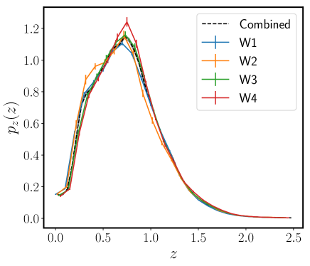
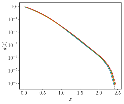
Figure 1: Left panel: Redshift probability density distribution of galaxies in the W1, W2, W3 and W4 fields of the CFHTLenS as a function of redshift (i.e. $dN/dz/N_{\rm TOT}$ versus $z$). The coloured solid lines show the results for the individual fields and the dashed black line shows the total for the combined fields. error bars and the grey shaded band show the 1$\sigma$ confidence regions, obtained from a jackknife resampling of the survey area. Right panel: The weight function $g(\chi(z))$ given in Eq. (3) as a function of redshift for the four CFHTLenSfields and the combined set. Line styles and colours are as in the left panel.

2.2 Tangential and cross shear

Owing to the fact that gravity only ‘excites’ certain shear patterns we wish to rotate the shear into the frame where we can more easily separate out the these modes. This is done by decomposing the shear into ‘tangential’ and ‘cross’ components. Consider the shear field at a position vector ${\bm{\theta}}+{\bm{\theta}}_{0}$, where ${\bm{\theta}}_{0}$ is an arbitrary location and ${\bm{\theta}}$ is a radial vector centred on ${\bm{\theta}}_{0}$. We may rotate the shear field by the polar angle of the separation vector ${\bm{\theta}}$ to obtain the tangential and cross components (Bartelmann & Schneider, 2001):

$$\gamma_{\rm t}({\bm{\theta}};{\bm{\theta}}_{0}) \equiv-\Re\left[\gamma(\bm{\theta}+{\bm{\theta}}_{0}){\rm e}^{-2i\phi}\right]\ ;$$ (4)

$$\gamma_{\times}({\bm{\theta}};{\bm{\theta}}_{0}) \equiv-\Im\left[\gamma(\bm{\theta}+{\bm{\theta}}_{0}){\rm e}^{-2i\phi}\right]\ ,$$ (5)

where $\phi$ is the polar angle associated with the vector ${\bm{\theta}}$. The main advantage of this transformation is that for an axially-symmetric mass distribution, the shear is always tangentially aligned relative to the direction towards the origin of the mass distribution and the cross component will vanish. This result is not true for any randomly selected point for the origin. However, if we average the tangential shear over a ring it can be related to the enclosed surface mass density $\overline{\kappa}$: $\left<\gamma_{\rm t}({\bm{\theta}};{\bm{\theta}}_{0})\right>_{\rm circ}=\overline{\kappa}(\theta;{\bm{\theta}}_{0})-\left<\kappa(\theta;{\bm{\theta}}_{0})\right>_{\rm circ}$. On the other hand, if we ring average the cross-shear it will vanish: $\left<\gamma_{\times}({\bm{\theta}};{\bm{\theta}}_{0})\right>_{\rm circ}=0$ (Kaiser, 1995; Schneider, 1996).

3 Aperture mass measures for cosmic shear

In this paper we are primarily concerned with the statistical properties of the ring averaged tangential shear integrated over a filter function with compact support – the aperture mass.

3.1 Aperture Mass

Aperture mass was developed by Schneider (1996) as a technique for using a weighted set of measured shears within a circular region to estimate the enclosed projected mass overdensity. It can be defined as follows: consider an angular position vector in the survey ${\bm{\theta}}_{0}$, and let us compute the tangential shear field around this point. Aperture mass is now defined as the convolution of the tangential shear with a circularly-symmetric filter function $Q$, with a characteristic scale ${\vartheta}$, above which the filter functions are typically set to zero. It can be expressed as:

$${\mathcal{M}}_{\rm ap}({\bm{\theta}}_{0};{\vartheta})\equiv\int_{{\mathbb{R}^{2}}}{{\rm d}^{2}\bm{\theta}}_{1}\gamma_{{\rm t}}({\bm{\theta}}_{1};{\bm{\theta}}_{0})Q(|{\bm{\theta}}_{1}-{\bm{\theta}}_{0}|;{\vartheta})\ .$$ (6)

In a similar vain one can also define the cross component of aperture mass, which we refer to as ‘map-cross’:

$$\mathcal{M}_{\times}({\bm{\theta}}_{0};{\vartheta})\equiv\int_{{\mathbb{R}^{2}}}{{\rm d}^{2}\bm{\theta}}_{1}\gamma_{\times}({\bm{\theta}}_{1};{\bm{\theta}}_{0})Q(|{\bm{\theta}}_{1}-{\bm{\theta}}_{0}|;{\vartheta})\ .$$ (7)

In the absence of systematic errors (B-modes) in the lensing data, map-cross should vanish. ${\mathcal{M}}_{\rm ap}$ and $\mathcal{M}_{\times}$ are therefore said to be E/B decomposed (Schneider, van Waerbeke & Mellier, 2002).

As was proven by Schneider (1996), owing to the fact that the shear and convergence are sourced by the same scalar potential, one can derive an equivalent relation to that above, but computed by convolving the convergence $\kappa$ with a different filter function $U$:

$${\mathcal{M}}_{\rm ap}({\bm{\theta}}_{0};{\vartheta})=\int_{{\mathbb{R}^{2}}}{{\rm d}^{2}\bm{\theta}}_{1}\kappa({\bm{\theta}}_{1})U(\left|{\bm{\theta}}_{1}-{\bm{\theta}}_{0}\right|;{\vartheta})\ .$$ (8)

It is important to note that the filter functions $Q$ and $U$ are not independent of one another, but are related (Schneider, 1996):

$$Q(\theta;{\vartheta}) =\frac{2}{\theta^{2}}\int_{0}^{\theta}{\rm d}\theta^{\prime}\theta^{\prime}U(\theta^{\prime};{\vartheta})-U(\theta;{\vartheta})\ ;$$ (9)

$$U(\theta;{\vartheta}) =2\int_{\theta}^{\infty}\frac{{\rm d}\theta^{\prime}}{\theta^{\prime}}Q(\theta^{\prime};{\vartheta})-Q(\theta;{\vartheta})\ .$$ (10)

Also, it is worth noting that the $U$ filter is a compensated function (Bartelmann & Schneider, 2001).

For this work we will be using a polynominal filter function introduced in Schneider et al. (1998):

$$Q(\theta;{\vartheta})=\frac{6}{\pi{\vartheta}^{2}}\left(\frac{\theta}{{\vartheta}}\right)^{2}\left[1-\left(\frac{\theta}{{\vartheta}}\right)^{2}\right]\mathcal{H}({\vartheta}-\theta)\ ,$$ (11)

where ${\mathcal{H}}(x)$ is the Heaviside function.

3.2 Aperture mass variance

For cosmic shear, the expectation of the aperture mass around a randomly selected point vanishes, since $\left<\kappa\right>=\left<\gamma_{\rm t}\right>=0$. Thus, the lowest order non-zero quantity of interest is the variance. Using Eq. (6) the variance of the aperture mass can be written as:

$$\left<\mathcal{M}_{\rm ap}^{2}\right>({\bm{\theta}}_{0};{\vartheta}) =\int_{{\mathbb{R}^{2}}}{{\rm d}^{2}\bm{\theta}}_{1}{{\rm d}^{2}\bm{\theta}}_{2}\left<\gamma_{{\rm t}}({\bm{\theta}}_{1};{\bm{\theta}}_{0})\gamma_{{\rm t}}({\bm{\theta}}_{2};{\bm{\theta}}_{0})\right>$$

$$\times Q(|{\bm{\theta}}_{1}-{\bm{\theta}}_{0}|;{\vartheta})Q(|{\bm{\theta}}_{2}-{\bm{\theta}}_{0}|;{\vartheta})\ .$$ (12)

Using Eq. (8) we see that this can be equivalently written as:

$$\left<\mathcal{M}_{\rm ap}^{2}\right>({\bm{\theta}}_{0};{\vartheta}) =\int_{{\mathbb{R}^{2}}}{{\rm d}^{2}\bm{\theta}}_{1}{{\rm d}^{2}\bm{\theta}}_{2}\left<\kappa({\bm{\theta}}_{1})\kappa({\bm{\theta}}_{2})\right>$$

$$\times U(\left|{\bm{\theta}}_{1}-{\bm{\theta}}_{0}\right|;{\vartheta})U(\left|{\bm{\theta}}_{2}-{\bm{\theta}}_{0}\right|;{\vartheta})\ .$$ (13)

The Fourier transform of the convergence, $\tilde{\kappa}$, is defined as follows:

$$\kappa({\bm{\theta}}) \equiv\int_{{\mathbb{R}^{2}}}\frac{{{\rm d}^{2}\bm{\ell}}}{(2\pi)^{2}}\tilde{\kappa}({\bm{\ell}}){\rm e}^{-i{\bm{\ell}}\cdot{\bm{\theta}}}.$$ (14)

On using the above transform in Eq. (13) we find:

$$\left<\mathcal{M}_{\rm ap}^{2}\right>({\bm{\theta}}_{0};{\vartheta}) =\int_{{\mathbb{R}^{2}}}{{\rm d}^{2}\bm{\theta}}_{1}{{\rm d}^{2}\bm{\theta}}_{2}\int_{{\mathbb{R}^{2}}}\frac{{{\rm d}^{2}\bm{\ell}}_{1}}{(2\pi)^{2}}\frac{{{\rm d}^{2}\bm{\ell}}_{2}}{(2\pi)^{2}}\left<\tilde{\kappa}({\bm{\ell}}_{1})\tilde{\kappa}({\bm{\ell}}_{2})\right>$$

$$\times{\rm e}^{-i({\bm{\ell}}_{1}\cdot{\bm{\theta}}_{1}+{\bm{\ell}}_{2}\cdot{\bm{\theta}}_{2})}U(\left|{\bm{\theta}}_{1}-{\bm{\theta}}_{0}\right|;{\vartheta})U(\left|{\bm{\theta}}_{2}-{\bm{\theta}}_{0}\right|;{\vartheta})\ .$$ (15)

We next use the statistical homogeneity and isotropy of the correlations of $\kappa({\bm{\theta}})$ to define the convergence power spectrum:

$$\left<\tilde{\kappa}({\bm{\ell}}_{1})\tilde{\kappa}({\bm{\ell}}_{2})\right>=(2\pi)^{2}\delta^{\rm D}({\bm{\ell}}_{1}+{\bm{\ell}}_{2})C_{\kappa\kappa}(\ell_{1})\ .$$ (16)

On inserting this into Eq. (15) and integrating over the Dirac delta function we see that the aperture mass variance can be written:

$$\left<\mathcal{M}_{\rm ap}^{2}\right>({\vartheta}) =\int_{{\mathbb{R}^{2}}}\frac{{{\rm d}^{2}\bm{\ell}}}{(2\pi)^{2}}C_{\kappa\kappa}(\ell)\left|\tilde{U}({\bm{\ell}};{\vartheta})\right|^{2}\ .$$ (17)

where

$$\tilde{U}({\bm{\ell}};{\vartheta})=\int_{{\mathbb{R}^{2}}}{\rm d}^{2}{\bm{y}}\ {\rm e}^{i{\bm{\ell}}\cdot{\bf y}}U(\left|{\bf y}\right|;{\vartheta})\ .$$ (18)

To progress we need to relate the convergence power to the matter power spectrum $P$ that, in the small-scale limit and under the Limber approximation, can be related to the convergence power spectrum as:

$$C_{\kappa}(\ell) =\frac{9}{4}\Omega_{\rm m,0}^{2}\left(\frac{H_{0}}{c}\right)^{4}\int_{0}^{\chi_{\rm H}}{\rm d}\chi\frac{g^{2}(\chi)}{a^{2}(\chi)}P\left(\frac{\ell}{\chi},\chi\right)\ .$$ (19)

On inserting this relation into Eq. (17) and using the Schneider polynomial filter function Eq. (11) such that $\tilde{U}(\ell;{\vartheta})=24J_{4}(\ell{\vartheta})/(\ell{\vartheta})^{2}$ we have (Schneider et al., 1998):

$$\left<\mathcal{M}_{\rm ap}^{2}\right>({\bm{\theta}}_{0};{\vartheta}) =\frac{1}{{\vartheta}^{2}}\frac{24^{2}}{2\pi}\frac{9}{4}\Omega_{\rm m,0}^{2}\left(\frac{H_{0}}{c}\right)^{4}\int_{0}^{\chi_{\rm H}}{\rm d}\chi\frac{g^{2}(\chi)}{a^{2}(\chi)}$$

$$\times\int_{0}^{\infty}{\rm d}y\frac{J_{4}^{2}(y)}{y^{3}}P\left(\frac{y}{{\vartheta}\chi},\chi\right)\ .$$ (20)

3.3 Aperture mass variance from shear correlation functions

As discussed earlier, the standard method for estimating the aperture mass variance is through the two-point shear correlation functions. Let us make that connection explicit. The complex shear field has two non-vanishing two-point correlation functions that can be written in terms of its tangential and cross-components as (Schneider, van Waerbeke & Mellier, 2002):

$$\xi_{+}(\theta) \equiv\left<\gamma_{\rm t}({\bm{\theta}}_{1};{\bm{\theta}}_{1})\gamma_{\rm t}({\bm{\theta}}_{2};{\bm{\theta}}_{1})\right>+\left<\gamma_{\times}({\bm{\theta}}_{1};{\bm{\theta}}_{1})\gamma_{\times}({\bm{\theta}}_{2};{\bm{\theta}}_{1})\right>\ ;$$ (21)

$$\xi_{-}(\theta) \equiv\left<\gamma_{\rm t}({\bm{\theta}}_{1};{\bm{\theta}}_{1})\gamma_{\rm t}({\bm{\theta}}_{2};{\bm{\theta}}_{1})\right>-\left<\gamma_{\times}({\bm{\theta}}_{1};{\bm{\theta}}_{1})\gamma_{\times}({\bm{\theta}}_{2};{\bm{\theta}}_{1})\right>\ ,$$ (22)

where in this subsection $\theta\equiv|{\bm{\theta}}_{1}-{\bm{\theta}}_{2}|$. It can be shown that $\xi_{+}$ and $\xi_{-}$ can be written in terms of the convergence power spectrum as:

$$\xi_{+}(\theta) =\int_{{\mathbb{R}^{2}}}\frac{{{\rm d}^{2}\bm{\ell}}}{(2\pi)^{2}}C_{\kappa\kappa}(\ell)J_{0}(\ell\theta)\ ;$$ (23)

$$\xi_{-}(\theta) =\int_{{\mathbb{R}^{2}}}\frac{{{\rm d}^{2}\bm{\ell}}}{(2\pi)^{2}}C_{\kappa\kappa}(\ell)J_{4}(\ell\theta)\ .$$ (24)

Using the orthogonality of the Bessel functions we can invert the above expressions to obtain the convergence power spectrum:

$$C_{\kappa\kappa}(\ell) =2\pi\int_{0}^{\infty}{\rm d}\theta\theta\xi_{+}(\theta)J_{0}(\ell\theta)\ ;$$ (25)

$$=2\pi\int_{0}^{\infty}{\rm d}\theta\theta\xi_{-}(\theta)J_{4}(\ell\theta)\ .$$ (26)

The important consequence of the above relations is that we can now rewrite the aperture mass variance using the shear correlation functions. On substitution of Eqs. (25) and (26) into Eq. (17) one finds (Schneider, van Waerbeke & Mellier, 2002):

$$\left<\mathcal{M}_{\rm ap}^{2}\right>({\bm{\theta}}_{0};{\vartheta}) =\int_{{\mathbb{R}^{2}}}\frac{{{\rm d}^{2}\bm{\ell}}}{(2\pi)^{2}}\left|\tilde{U}({\bm{\ell}};{\vartheta})\right|^{2}\pi\left[\int_{0}^{\infty}{\rm d}\theta\theta\xi_{+}(\theta)J_{0}(\ell\theta)\right.$$

$$\left.+\int_{0}^{\infty}{\rm d}\theta\theta\xi_{-}(\theta)J_{4}(\ell\theta)\right]\ .$$ (27)

On reordering the integrals over $\ell$ and $\theta$, we see that the above can be written more compactly as:

$$\left<\mathcal{M}_{\rm ap}^{2}\right>({\bm{\theta}}_{0};{\vartheta}) =\frac{1}{2{\vartheta}^{2}}\int_{0}^{\infty}{\rm d}\theta\theta\bigg{[}\xi_{+}(\theta)T_{+}(\theta|{\vartheta})$$

$$+\xi_{-}(\theta)T_{-}(\theta|{\vartheta})\bigg{]}\ ,$$ (28)

where

$$T_{+}(\theta|{\vartheta}) \equiv\int_{0}^{\infty}{\rm d}\ell\ell\left|\tilde{U}(\ell;{\vartheta})\right|^{2}J_{0}(\ell\theta)\ \ ,$$ (29)

$$T_{-}(\theta|{\vartheta}) \equiv\int_{0}^{\infty}{\rm d}\ell\ell\left|\tilde{U}(\ell;{\vartheta})\right|^{2}J_{4}(\ell\theta)\ .$$ (30)

Once again, on adopting the Schneider polynomial filter Eq. (11) we see that the above kernels have an analytic form (Schneider, van Waerbeke & Mellier, 2002):

$$T_{+}(y) =\frac{{\mathcal{H}}(2-y)}{100\pi}\bigg{[}240\left(2-15y^{2}\right)\cos^{-1}\left(\frac{y}{2}\right)+y\sqrt{4-y^{2}}$$

$$\times\left(120+2320y^{2}-754y^{4}+132y^{6}-9y^{8}\right)\bigg{]}\ ;$$ (31)

$$T_{-}(y) =\frac{192}{35\pi}y^{3}\left(1-\frac{y^{2}}{4}\right)^{7/2}{\mathcal{H}}(2-y)\ ,$$ (32)

where in the above $y\equiv\theta/{\vartheta}$.

There are several important things to note about this: first, for the case of the Schneider polynomial filter function, one needs to measure $\xi_{+}$ and $\xi_{-}$ over the range $\theta\in[0,2{\vartheta}]$, meaning that we need information from scales close to zero separation. The correlations on small scales can not be accurately measured and will be dominated by image blending issues and shape noise (Kilbinger, Schneider & Eifler, 2006). Second, the integration to obtain the variance from Eq. (28) can only be approximately done using a set of discrete bins which need to be sufficiently dense and non empty. The result of all of this is that there will be some amount of E/B leakage, which will lead to a suppression of the signal on small scales (Kilbinger, Schneider & Eifler, 2006). The first issue is also a problem for the direct estimator, but the second is not.

4 Estimating the aperture mass statistics

As discussed in the previous section, there are two approaches to estimating the aperture mass statistics. The correlation function approach outlined in the previous section has been studied in great detail. The direct estimator approach that we explore in this work has not been as well explored, we therefore now describe our extension of this approach in some detail.

4.1 The direct estimator for the aperture mass dispersion for a single field – including the source weights

Here we follow Schneider et al. (1998), but extend the work to include a set of arbitrary weights for each source galaxy. Let us first introduce the direct estimator of the aperture mass dispersion for a single field. Consider an aperture of angular radius ${\vartheta}$, centred on the position ${\bm{\theta}}_{0,k}$. The aperture contains $N_{k}$ galaxies with positions ${\bm{\theta}}_{i}$ with complex ellipticities $\epsilon_{i}$. For the case of weak lensing the observed ellipticities and intrinsic ellipticities $\epsilon_{i}^{(\rm s)}$ are approximately related though $\epsilon_{i}=\gamma_{i}+\epsilon_{i}^{(\rm s)}$. In complete analogy to the definition of tangential and cross shear defined in Eqs. (4) and (5) we define the same quantities for the tangential and cross components of ellipticity: $\epsilon_{\rm t}=-\Re\left[\epsilon\ {\rm e}^{-2i\phi}\right]$ and $\epsilon_{\times}=-\Im\left[\epsilon\ {\rm e}^{-2i\phi}\right]$, where the polar angle $\phi$ is relative to the origin ${\bm{\theta}}_{0,k}$. Our estimator for the aperture mass variance is defined as:

$$\widehat{{\mathcal{M}}_{\rm ap}^{2}({\vartheta}|\mn@boldsymbol{\theta}_{0,k})} :=(\pi{\vartheta}^{2})^{2}\ \frac{\sum_{i}^{N_{k}}\sum_{j\neq i}^{N_{k}}w_{i}\ w_{j}\ Q_{i}\ Q_{j}\epsilon_{{\rm t},i}\ \epsilon_{{\rm t},j}}{\sum_{i}^{N_{k}}\sum_{j\neq i}^{N_{k}}w_{i}w_{j}}\ ,$$ (33)

where $w_{i}$ are weights assigned to the $i$th galaxy, the $Q_{i}\equiv Q(|{\bm{\theta}}_{i}|;{\vartheta})$ and where $\epsilon_{{\rm t},i}$ is the observed tangential ellipticity of the $i$th galaxy measured with respect to the origin $\mn@boldsymbol{\theta}_{0,k}$. Note that since the double sum will occur repeatedly, we will use the short-hand notation $\sum_{i}^{N_{k}}\sum_{j\neq i}^{N_{k}}\rightarrow\sum_{i\neq j}$ for brevity. We will also suppress the origin $\mn@boldsymbol{\theta}_{0,k}$ and also take $N_{k}=N$.

We show that this provides an unbiased estimator for the true aperture mass dispersion. This can be done through applying three averaging processes: averaging over the intrinsic ellipticity distributions $A$; then the source galaxy positions $P$; and then the ensemble average over the cosmic fields $E$ (following the notation of Schneider et al., 1998). Ignoring the prefactor and the denominator for a moment, if we perform the $A$ average then we get:

$$A\left(\sum_{i\neq j}w_{i}w_{j}Q_{i}Q_{j}{\epsilon}_{{\rm t},{i}}{\epsilon}_{{\rm t},{j}}\right) =A\left(\sum_{i,j}w_{i}w_{j}Q_{i}Q_{j}{\epsilon}_{{\rm t},{i}}{\epsilon}_{{\rm t},{j}}\right)$$

$$-A\left(\sum_{i}w_{i}^{2}Q_{i}^{2}{\epsilon}_{{\rm t},{i}}^{2}\right)$$

$$=\sum_{i,j}w_{i}w_{j}Q_{i}Q_{j}\bigg{\{}{\gamma}_{{\rm t},{i}}{\gamma}_{{\rm t},{j}}+2{\gamma}_{{\rm t},{i}}\ A\left({\epsilon}_{{\rm t},{j}}^{(s)}\right)+A\left({\epsilon}_{{\rm t},{i}}^{(s)}{\epsilon}_{{\rm t},{j}}^{(s)}\right)\bigg{\}}$$

$$-\sum_{i}w_{i}^{2}Q_{i}^{2}\left\{{\gamma}_{{\rm t},{i}}^{2}+2\ {\gamma}_{{\rm t},{i}}\ A\left({\epsilon}_{{\rm t},{i}}^{(s)}\right)+A\left([{\epsilon}_{{\rm t},{i}}^{(s)}]^{2}\right)\right\}$$

$$=\sum_{i,j}w_{i}w_{j}Q_{i}Q_{j}\left\{{\gamma}_{{\rm t},{i}}{\gamma}_{{\rm t},{j}}+\frac{\sigma_{\epsilon}^{2}}{2}\delta^{K}_{ij}\right\}$$

$$-\sum_{i}w_{i}^{2}Q_{i}^{2}\left\{{\gamma}_{{\rm t},{i}}^{2}+\frac{\sigma_{\epsilon}^{2}}{2}\right\}$$

$$=\sum_{i\neq j}w_{i}w_{j}Q_{i}Q_{j}{\gamma}_{{\rm t},{i}}{\gamma}_{{\rm t},{j}}\ .$$ (34)

Note that in the above we assumed that each galaxies’ intrinsic ellipticity is indiviually drawn from the same Gaussian distribution $\mathcal{G}\left(0,\sigma^{2}_{\epsilon}\right)$ with zero mean and the shape noise $\sigma^{2}_{\epsilon}$ as variance, i.e. no intrinsic alignments. Next, we perform the average over the spatial positions of the source galaxies:

$$P\left(\sum_{i\neq j}w_{i}w_{j}Q_{i}Q_{j}\gamma_{{\rm t},i}\gamma_{{\rm t},j}\right) =\prod_{\alpha=1}^{N}\left\{\frac{{\rm d}^{2}{\bm{\theta}}_{\alpha}}{\pi{\vartheta}^{2}}\right\}$$

$$\times\sum_{i\neq j}w_{i}w_{j}Q_{i}Q_{j}\gamma_{{\rm t},i}\gamma_{{\rm t},j}$$

$$=\frac{\sum_{i\neq j}w_{i}w_{j}}{\left(\pi{\vartheta}^{2}\right)^{2}}\int_{\mathbb{R}^{2}}{\rm d}^{2}{\bm{\theta}}_{1}{\rm d}^{2}{\bm{\theta}_{2}}\ Q_{1}Q_{2}\gamma_{{\rm t},1}\gamma_{{\rm t},2}\ .$$ (35)

In the first step we took the joint PDF of spatial positions to be simply the product of the independent 1-point PDFs for a uniform random distribution. In the second step, on noting that $\gamma_{{\rm t},i}=\gamma_{{\rm t},i}({\bm{\theta}}_{i};{\bm{\theta}}_{0})$, where $\mathbf{\theta}_{0}$ is the same for all the galaxies, we used the fact that the spatial integral will yield the same result no matter of the indices - hence the change $(i,j)\rightarrow(1,2)$. In the last step, we integrated out the remaining PDFs and rewrote the domain. Finally, we perform the expectation over the cosmic fields:

$$E\left\{P\left[A\left(\widehat{{\mathcal{M}}_{\rm ap}^{2}({\vartheta})}\right)\right]\right\} =\frac{(\pi{\vartheta}^{2})^{2}}{\sum_{i\neq j}w_{i}w_{j}}\frac{\sum_{i\neq j}w_{i}w_{j}}{\left(\pi{\vartheta}^{2}\right)^{2}}$$

$$\times\int_{\mathbb{R}^{2}}{\rm d}^{2}{\bm{\theta}_{1}}{\rm d}^{2}{\bm{\theta}}_{2}\ Q_{1}Q_{2}\left<\gamma_{{\rm t},1}\gamma_{{\rm t},2}\right>$$

$$=\left<\mathcal{M}_{\rm ap}^{2}\right>\ .$$ (36)

In Appendix A we calculate the variance of the estimator Eq. (33) and, for a moment supressing $\vartheta$, we find that it can be written as:

$$\!\!{\rm Var}\left[\widehat{{\mathcal{M}}_{\rm ap}^{2}}\right] =\frac{\sum_{l\neq k\neq j\neq i}w_{i}w_{j}w_{k}w_{l}}{\left(\sum_{j\neq i}w_{i}w_{j}\right)^{2}}\left<{\mathcal{M}}_{\rm ap}^{4}\right>$$

$$+4\frac{\sum_{k\neq j\neq i}w_{i}^{2}w_{j}w_{k}}{\left(\sum_{j\neq i}w_{i}w_{j}\right)^{2}}\left<{\mathcal{M}}_{\rm ap}^{2}{\mathcal{M}}_{\rm s,2}\right>$$

$$+2\frac{\sum_{j\neq i}w_{i}^{2}w_{j}^{2}}{\left(\sum_{j\neq i}w_{i}w_{j}\right)^{2}}\left<{\mathcal{M}}_{\rm s,2}^{2}\right>$$

$$+\frac{2\sum_{k\neq i\neq j}w_{i}w_{j}^{2}w_{k}}{\left(\sum_{j\neq i}w_{i}w_{j}\right)^{2}}\sigma^{2}_{\epsilon}G\left<{\mathcal{M}}_{\rm ap}^{2}\right>$$

$$+\frac{2\sum_{j\neq i}w_{i}^{2}w_{j}^{2}}{\left(\sum_{j\neq i}w_{i}w_{j}\right)^{2}}\sigma^{2}_{\epsilon}G\left<{\mathcal{M}}_{s,2}\right>$$

$$+\frac{\sum_{j\neq i}w_{i}^{2}w_{j}^{2}}{2\left(\sum_{j\neq i}w_{i}w_{j}\right)^{2}}\sigma^{4}_{\epsilon}G^{2}-\left<{\mathcal{M}}_{\rm ap}^{2}\right>^{2},$$ (37)

where $G$ and ${\mathcal{M}}_{s,2}$ are as defined as:

$$\langle{\mathcal{M}}_{\rm s,2}\rangle(\vartheta) \equiv\pi{\vartheta}^{2}\int{\rm d}^{2}{\bm{\theta}}\ Q^{2}(|{\bm{\theta}}|;\vartheta)\langle\gamma^{2}_{\rm t}\rangle({\bm{\theta}})\ ;$$

$$G(\vartheta) \equiv\pi{\vartheta}^{2}\int{\rm d}^{2}\mn@boldsymbol{\theta}\ Q^{2}(|{\bm{\theta}}|;\vartheta)\ .$$ (38)

Importantly, in the limit where all of the source galaxy weights are equal we recover the expression derived in Schneider et al. (1998).

It is interesting to obtain an approximate form for the above variance. Firstly, let us consider the case where the number of galaxies per aperture is large such that $N\gg 1$, whereupon we see that all of the partial sums are approximately equivalent to the full sums, e.g. $\sum_{i}\sum_{j\neq i}w_{i}w_{j}\approx(\sum_{i}w_{i})^{2}$. Consequently, all of the prefactors involving the weights can be dramatically simplified to give:

$$\lim_{N\rightarrow\infty}{\rm Var}\left[\widehat{{\mathcal{M}}_{\rm ap}^{2}}\right] \approx\left<{\mathcal{M}}_{\rm ap}^{4}\right>+4S_{2}\left<{\mathcal{M}}_{\rm ap}^{2}{\mathcal{M}}_{\rm s,2}\right>+2S_{2}^{2}\left<{\mathcal{M}}_{\rm s,2}^{2}\right>$$

$$+2S_{2}\sigma^{2}_{\epsilon}G\left<{\mathcal{M}}_{\rm ap}^{2}\right>+2S_{2}^{2}\sigma^{2}_{\epsilon}G\left<{\mathcal{M}}_{s,2}\right>$$

$$+\frac{1}{2}S_{2}^{2}\sigma^{4}_{\epsilon}G^{2}-\left<{\mathcal{M}}_{\rm ap}^{2}\right>^{2}\ ,$$ (39)

where we defined $S_{2}\equiv\sum_{i}w_{i}^{2}/(\sum_{i}w_{i})^{2}$. Let us inspect the quantity $S_{2}$ in more detail: the Cauchy-Schwarz inequality tells us that $\left(\sum_{i}^{N}u_{i}v_{i}\right)^{2}\leq\sum_{i}^{N}u_{i}^{2}\sum_{j}^{N}v_{j}^{2}$, where the elements of the sets $\{u_{i}\}$ and $\{v_{i}\}$ are drawn from the reals. If we take $v_{i}=v$ for any $i$, then we see that $\left(\sum_{i}^{N}u_{i}\right)^{2}\leq\sum_{i}^{N}u_{i}^{2}N$, which in turn implies $\left<u\right>^{2}\leq\left<u^{2}\right>$. On applying this to our ratio $S_{2}$ we see that:

$$S_{2}\equiv\frac{1}{N}\frac{\overline{w^{2}}}{\overline{w}^{2}}\geq\frac{1}{N}$$ (40)

where $\overline{w^{2}}=\sum_{i}w_{i}^{2}/N$ and $\overline{w}=\sum_{i}w_{i}/N$. This insight leads us to make our next approximation, since $\mathcal{M}_{s,2}\sim{\mathcal{M}}^{2}_{\rm ap}$ we see that $S_{2}\mathcal{M}_{s,2}\ll{\mathcal{M}}^{2}_{\rm ap}$, since $S_{2}\propto 1/N$. This, then, leads us to write:

$$\lim_{N\rightarrow\infty}{\rm Var}\left[\widehat{{\mathcal{M}}_{\rm ap}^{2}}\right] \approx\left<{\mathcal{M}}_{\rm ap}^{4}\right>+2S_{2}\sigma^{2}_{\epsilon}G\left<{\mathcal{M}}_{\rm ap}^{2}\right>$$

$$+\frac{1}{2}S_{2}^{2}\sigma^{4}_{\epsilon}G^{2}-\left<{\mathcal{M}}_{\rm ap}^{2}\right>^{2}\ .$$ (41)

Thirdly, let us further assume that the underlying shear field is Gaussian and hence $\left<{\mathcal{M}}_{\rm ap}^{4}\right>=3\left<{\mathcal{M}}_{\rm ap}^{2}\right>^{2}$. Under these circumstances, which will be fulfilled for large apertures, the variance can be written as:

$${\rm Var}\left[\widehat{{\mathcal{M}}_{\rm ap}^{2}}\right] \approx 2\left<{\mathcal{M}}_{\rm ap}^{2}\right>^{2}+2S_{2}\sigma^{2}_{\epsilon}G\left<{\mathcal{M}}_{\rm ap}^{2}\right>+\frac{1}{2}S_{2}^{2}\sigma^{4}_{\epsilon}G^{2}$$

$$=\left(\sqrt{2}\left<{\mathcal{M}}_{\rm ap}^{2}\right>+\frac{1}{\sqrt{2}}S_{2}G\sigma^{2}_{\epsilon}\right)^{2}\ .$$ (42)

The first term in the bracket is cosmic variance and the last term denotes the shape noise contribution.

The left panel of Figure 2 shows the error on a given estimate from a single aperture, using Eq. (42). The right panel shows the corresponding prediction of the signal-to-noise on the aperture mass variance, per aperture, again using Eq. (42). In order to generate these prediction we have used (20) as a model for the cosmic variance contribution.

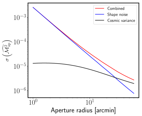
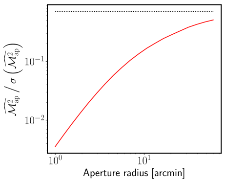
Figure 2: Left panel: Contributions to the variance of the estimate of the aperture mass dispersion in the CFHTLenS data. We show the two contributions to the variance as predicted from (42) as well as the combined result. Note that in adopting (42) we have assumed that the convergence is Gaussianly distributed. Right panel: The theoretical signal-to-noise per aperture as a function of the aperture size $\vartheta$ in the CFHTLenS data. The black dotted line shows the cosmic variance limit.

4.2 Acceleration of the direct estimator

If we were to naively implement the direct estimator approach as given by Eq. (33) then we see that in order to compute the estimate of the variance for a single aperture we need to compute the sum from $N(N-1)$ galaxies. Thus one might conclude that the method scales as typical $N^{2}$ pair counting approach for galaxies inside the aperture. However, we now show that the method can be made to scale linearly with the number of galaxies. Let us consider again the estimator from Eq. (33), and we notice that if we put back the term that has $i\neq j$ and explicitly subtract it then we have:

$$\widehat{{\mathcal{M}}_{\rm ap}^{2}({\vartheta}|{\bm{\theta}}_{0,k})} =(\pi{\vartheta}^{2})^{2}\frac{\sum_{i,j}w_{i}\ w_{j}\ Q_{i}\ Q_{j}\ \epsilon_{{\rm t},i}\epsilon_{{\rm t},j}}{\sum_{i\neq j}w_{i}w_{j}}$$

$$-(\pi{\vartheta}^{2})^{2}\ \frac{\sum_{i}w_{i}^{2}\ Q_{i}^{2}\epsilon^{2}_{t,i}}{\sum_{i\neq j}w_{i}w_{j}}\ .$$ (43)

If we now introduce the estimators for aperture mass and $\mathcal{M}_{s,2}$ as discretised versions of their definition,

$$\widehat{{\mathcal{M}}_{\rm ap}({\vartheta}|{\bm{\theta}}_{0,k})} \equiv(\pi{\vartheta}^{2})\frac{\sum_{i}w_{i}\ Q_{i}\epsilon_{{\rm t},i}}{\sum_{i}w_{i}}$$ (44)

$$\widehat{{\mathcal{M}}_{\rm s,2}({\vartheta}|{\bm{\theta}}_{0,k})} \equiv(\pi{\vartheta}^{2})\frac{\sum_{i}w_{i}^{2}\ Q_{i}^{2}\epsilon_{{\rm t},i}^{2}}{\sum_{i}w_{i}^{2}}\ ,$$ (45)

we see that Eq. (43) can be rewritten as:

$$\widehat{{\mathcal{M}}_{\rm ap}^{2}({\vartheta}|{\bm{\theta}}_{0,k})} =\frac{1}{1-S_{2}}\left(\frac{\pi{\vartheta}^{2}\sum_{i}w_{i}\ Q_{i}\epsilon_{{\rm t},i}}{\sum_{i}w_{i}}\right)^{2}$$

$$-\frac{\pi{\vartheta}^{2}}{\frac{1}{S_{2}}-1}\ \pi{\vartheta}^{2}\ \frac{\sum_{i}w_{i}^{2}\ Q_{i}^{2}\epsilon_{{\rm t},i}^{2}}{\sum_{i}w_{i}^{2}}$$

$$=\frac{1}{1-S_{2}}\left[(\widehat{{\mathcal{M}}_{\rm ap}})_{k}^{2}-S_{2}\pi{\vartheta}^{2}(\widehat{{\mathcal{M}}_{\rm s,2}})_{k}\right]\ ,$$ (46)

where for brevity we used the notation $(\widehat{{\mathcal{M}}_{\rm ap}})_{k}\equiv\widehat{{\mathcal{M}}_{\rm ap}({\vartheta}|{\bm{\theta}}_{0,k})}$ and $(\widehat{{\mathcal{M}}_{\rm s,2}})_{k}\equiv\widehat{{\mathcal{M}}_{\rm s,2}({\vartheta}|{\bm{\theta}}_{0,k})}$. Note that both terms in the brackets receive an identical contribution of shape noise, hence the second term should not be neglected.

In general, the estimator Eq. (46) is mathematically identical to that of Eq. (33) and therefore is also an unbiased estimator for the variance of the aperture mass. However, algorithmically it has a significant advantage in that it is linear in the number of galaxies. This owes to the fact that all of the terms on the right-hand-side of Eq. (46) are linear in $N$. For example, the estimate of $(\widehat{{\mathcal{M}}_{\rm ap}})_{k}$ is linear, so too are the correction factors $(\widehat{{\mathcal{M}}_{\rm s,2}})_{k}$ and $S$. As we will show in the second paper in this series (Porth et al., in prep.), it can be shown that this can be naturally extended to higher order aperture mass statistics. This acceleration of the method to linear order opens the door to a significant advantage in speed for estimation of aperture mass statistics at all order.

4.3 Extending the estimate to an ensemble of fields

The estimator Eq. (46) is for a single aperture $k$ and as such will provide a single low-signal-to-noise, albeit unbiased, estimate. We now wish to make use of the full area of the survey available to us. We are therefore confronted as to how to best achieve this. As proposed by Schneider et al. (1998), one simple approach would be to sample well seperated apertures such that the shear in one field is statistically independent from another. This would yield the estimator:

$$\widehat{{\mathcal{M}}_{\rm ap}^{2}({\vartheta})}=\frac{\sum_{k}{\mathcal{W}}_{k}\widehat{{\mathcal{M}}_{\rm ap}^{2}({\vartheta}|\mn@boldsymbol{\theta}_{0,k})}}{\sum_{k}{\mathcal{W}}_{k}}\ ,$$ (47)

where ${\mathcal{W}}_{k}$ are weights and the sum extends over the $N_{\rm ap}$ apertures. Since the estimates can be considered to be statistically independent then the noise can be minimised by choosing the weights to be given by:

$${\mathcal{W}}_{k}\propto\frac{1}{{\rm Var}\left[\widehat{{\mathcal{M}}_{\rm ap}^{2}({\vartheta}|\mn@boldsymbol{\theta}_{0,k})}\right]}\ .$$ (48)

However, this approach would be suboptimal in that it does not take advantage of the full area of the survey. In this case, the signal-to-noise on the estimate for the full field can be achieved by multiplying the estimates for the aperture mass variance per single aperture by the square root of the number of independent apertures.

A much better approach, which makes better use of the full survey area, is to oversample the apertures. Since the estimate for the survey is still given by Eq. (47) and since it is a linear combination of the estimates for the single field, it too is unbiased:

$$\left<\widehat{{\mathcal{M}}_{\rm ap}^{2}({\vartheta})}\right> =\frac{\sum_{k}{\mathcal{W}}_{k}\left<\widehat{{\mathcal{M}}_{\rm ap}^{2}({\vartheta}|\mn@boldsymbol{\theta}_{0,k})}\right>}{\sum_{k}{\mathcal{W}}_{k}}$$

$$=\left<\widehat{{\mathcal{M}}_{\rm ap}^{2}({\vartheta})}\right>\frac{\sum_{k}{\mathcal{W}}_{k}}{\sum_{k}{\mathcal{W}}_{k}}=\left<{\mathcal{M}}_{\rm ap}^{2}({\vartheta})\right>\ .$$ (49)

However, the variance of the estimate for the survey is no longer trivial to determine. This in turn means that the weights ${\mathcal{W}}_{k}$ from Eq. (48) are no longer optimal. Computing the optimal weights will be further complicated if we include incomplete apertures in the estimate – which we discuss next.

4.4 Allowing incomplete aperture coverage to increase estimator efficiency

We next turn to the problem of aperture completeness. In real surveys there are regions of the survey that are masked out due to bright stars, chip gaps and the survey boundaries. The question now arises: what do we do if an aperture has some fraction of its area overlapping with the mask? The simple answer would be that we exclude all such apertures from the estimator. The problem with this approach is that depending on the size of the aperture this may significantly impact the available survey area from which to compute the estimate and thus make the approach sub-optimal. Here we will explore the idea of effectively including all apertures that fit within the survey boundary, but apply weights to each of the form:

$${\mathcal{W}}_{k}=f(c_{k},{\rm Var},\dots)\ ,$$ (50)

where $c_{k}\equiv A_{k}/A$ is the completeness factor for the $k$th aperture, where $A_{k}$ is the available area of the aperture and $A$ is the unmasked area of the aperture, such that we have $c_{k}\leq 1$. $\rm Var$ is related to the variance of the estimate in the aperture. The ellipsis denotes that in general the weights could depend on other factors. In this work we will explore three distinct choices:

$${\mathcal{W}}^{(1)}_{k} ={\mathcal{H}}\left(c_{k}-\alpha\right);$$ (51)

$${\mathcal{W}}^{(2)}_{k} ={\mathcal{H}}\left(c_{k}-0\right){\rm Var}\left[\left<\widehat{{\mathcal{M}}_{\rm ap}^{2}({\vartheta}|\bm{\theta}_{0,k})}\right>\right]^{-1};$$ (52)

$${\mathcal{W}}^{(3)}_{k} ={\mathcal{H}}\left(c_{k}-\alpha\right){\rm Var}\left[\left<\widehat{{\mathcal{M}}_{\rm ap}^{2}({\vartheta}|\bm{\theta}_{0,k})}\right>\right]^{-1},$$ (53)

The first case corresponds to accepting all apertures whose completeness factor $c_{k}\geq\alpha$ and for those that do we combine them in a simple average with equal weights to arrive at our estimate for $\widehat{{\mathcal{M}}_{\rm ap}^{2}}$. The second case corresponds to accepting all apertures, irrespective of the completeness factor, but combining all of the estimates using an inverse variance weighted estimate, where the variance is approximated by Eq. (42). The third case is simply the product of the first and second case.

It is important to note that unless $\alpha=1$ our estimator given by Eq. (47) will formally become biased. This means that we will expect some leakage of E/B modes. Postponing a thorough analytical and numerical analysis of incomplete aperture coverage and de-biasing strategies to a companion paper, we will content our selves by investigating the degree of bias that is introduced by computing the aperture-cross statistics. For reference, these are defined in direct analogy with Eq. (33):

$$\widehat{{\mathcal{M}}_{\times}^{2}({\vartheta}|\mn@boldsymbol{\theta}_{0,k})} :=(\pi{\vartheta}^{2})^{2}\ \frac{\sum_{i\neq j}w_{i}\ w_{j}\ Q_{i}\ Q_{j}\ \epsilon_{\times,i}\ \epsilon_{\times,j}}{\sum_{i\neq j}w_{i}w_{j}}\ .$$ (54)

It can be proven that the expectation of this estimator vanishes; that is provided we have no bias in the estimate we have $\left<\widehat{{\mathcal{M}}_{\times}^{2}({\vartheta}|\mn@boldsymbol{\theta}_{0,k})}\right>=0$. However, the variance of the estimator does not vanish and it should be given by the pure shape noise contribution to Eq. (37). Under the approximations of Eq. (42) this is: $\frac{1}{2}{\rm Var}\left[\widehat{{\mathcal{M}}_{\times}^{2}({\vartheta})}\right]\approx S^{2}\sigma^{4}_{\epsilon}G^{2}$ per aperture.

Finally, before moving on, we note that it is important to appreciate that the weights ${\mathcal{W}}_{k}$ apply to how different fields are combined, and that the weights $w_{i}$ from Eq. (33) apply to how the source galaxies are combined in arriving at an estimate for a single field. We assume that these latter weights have been pre-computed by the method for estimating galaxy ellipticities.

4.5 Estimating computational complexity for evaluation of the direct estimator for $\widehat{{\mathcal{M}}_{\rm ap}^{2}}$

Before moving on to the computation of the estimator with real data let us estimate the computational cost for an evaluation of ${\mathcal{M}}_{\rm ap}^{2}$. As described above, the actual implementation is built from a series of algorithmic blocks.

1. We first construct a KD-tree data structure for the galaxy catalogue.

2. The full survey is tiled with overlapping apertures, where the centres are separated by a distance $d$.

3. The aperture coverage map is computed to give the $c_{k}$ values for every aperture.

4. For apertures that pass the selection cut (${\mathcal{H}}(c_{k}-\alpha)$), a KD-tree range search locates all particles that lie inside the aperture radius ${\vartheta}$.

5. Estimate the aperture mass statistics and its variance according to Eq. (37) for the $k$th aperture.

6. Combine the $N_{\rm ap}$ estimates through a weighted mean of the resulting estimates.

In the above algorithm we shall assume that Steps (i)–(iii), and Step (vi) are performed once and therefore are not the limiting factors for the execution of the code. We do note, however, that the construction of the KD-tree may have a large memory footprint and will take some non-negligible time for the initial construction. The parts of the method that require some consideration are Steps (iv) and (v).

Step (iv) is a range search routine and Step (v) is a routine that evaluates the sums in Eq. (46). To compute the complexity for these steps we first identify some parameters: let $p$ specify the order of the statistics; ${\vartheta}$ describe the aperture radius; and $\zeta$ be a parameter that determines the spacing $d$ between apertures: $d\equiv{\vartheta}/\zeta$. We note that for a non-overlapping field of apertures whose circumferences just touch each other, we would set $\zeta=1/2$. Further, the number of apertures is thus a function of ${\vartheta}$ and $\zeta$, $N_{\rm ap}({\vartheta},\zeta)$. The order for the complexity can thus be computed as follows:

$$\mathcal{O}(\widehat{{\mathcal{M}}_{\rm ap}^{p}}|p,{\vartheta},\zeta) =\sum_{k=1}^{N_{\rm ap}({\vartheta},\zeta)}\bigg{[}\mathcal{O}({\rm range\ search}|N_{k},N_{\rm nodes},{\vartheta})$$

$$\ \ +\mathcal{O}({\rm compute\ statistic}|N_{k},p)\bigg{]}$$

$$\approx N_{\rm ap}({\vartheta},\zeta)\bigg{[}\mathcal{O}({\rm range\ search}|\overline{N},N_{\rm Tot},{\vartheta})$$

$$\ \ +\overline{N}\mathcal{O}({\rm compute\ statistic}|N=1,p)\bigg{]}\ .$$ (55)

The first thing to notice is that the number of apertures scales all of the computations, so if we fix the parameter $\zeta$, then the total number of apertures will scale as $N_{\rm ap}\propto\Omega_{\rm s}/{\vartheta}^{2}$, where $\Omega_{\rm s}$ is the survey area. The first term in the square brackets gives the computational time for a range search to deliver back the $N_{k}$ galaxies in the aperture. If the distribution of source galaxies is roughly randomly distributed on the sky, then we make the approximation $N_{k}\approx\overline{N}=N_{\rm Tot}A/\Omega_{\rm s}$. Each such range search operation then takes of the order $\mathcal{O}(\log N_{\rm Tot})$ time to execute, but this factor will also scale with the aperture radius and how clustered the source galaxy data are, and also the depth we need to go in the tree walk.

Considering the second term in square brackets, this is the required time for computation of the estimate for the $p$th order aperture mass statistic. As was described earlier for $\widehat{{\mathcal{M}}_{\rm ap}^{2}}$, the estimator scales linearly with the number of galaxies in the aperture, thus in the second line we simply scale up the complexity to estimate the statistic for a single galaxy by the number of galaxies in the aperture. As we will explore in our companion paper, owing to this linear scaling, there is no additional overhead in extending the method to compute higher order statistics, beyond the variance, such as the skewness $p=3$ and kurtosis $p=4$.

5 Application to the CFHTLenS data

We now turn to estimating the aperture mass variance in the CFHTLenS data and in a large series of mocks generated by ray-tracing through $N$-body simulations.

5.1 CFHTLenS shear data

The Canada-France-Hawaii Telescope Lensing Survey (hereafter CFHTLenS) is a weak lensing survey that was completed around 2010. It covers 154 ${\rm deg}^{2}$ of the sky in five optical bands $\{u^{*},\ g^{\prime},\ r^{\prime},\ i^{\prime},\ z^{\prime}\}$ with a $\sim 5\sigma$ point source limiting magnitude in the $i^{\prime}$ band of $i^{\prime}_{\rm AB}\sim 25.5$. The survey measures galaxy ellipticities for use in weak lensing analysis from multicolour data obtained as part of the CFHT Legacy Survey. The survey data is distributed into four well spaced fields, three of which (W1, W2 & W4) lie close to the equatorial plane, and the third (W3) lies at high declination. Full details of the survey can be found in Heymans et al. (2012).

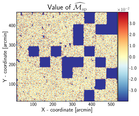
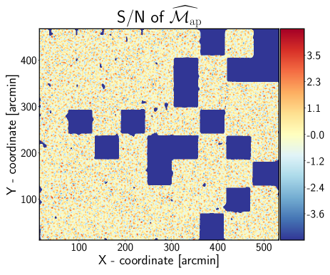
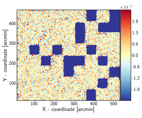
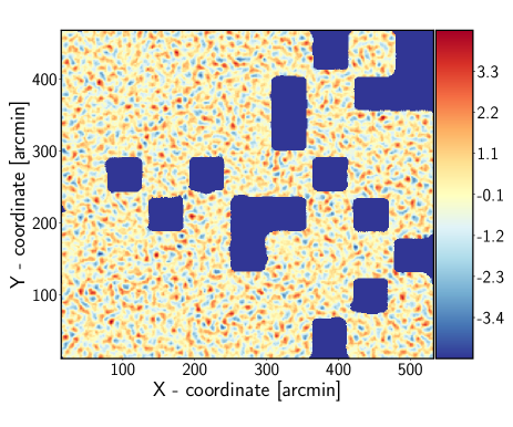
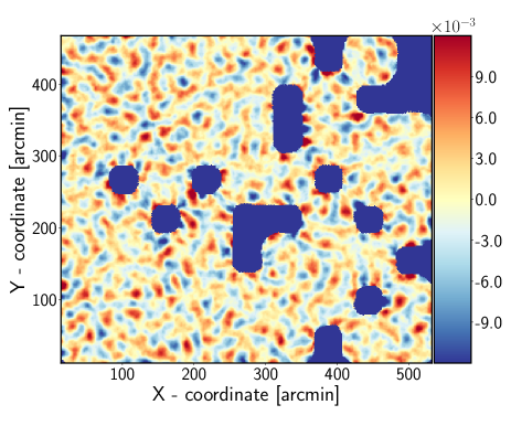
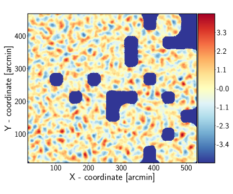
Figure 3: Mass related maps measured from the W1 field of the CFHTLenS data. The x- and y-axes show the right-ascension and declination of the survey, in arcminutes. The left and right columns show the results for the aperture mass (${\mathcal{M}_{\rm ap}}({\bm{\theta}}_{0}|{\vartheta})$) and the corresponding signal-to-noise ratio. The top, middle and bottom rows show the results for aperture radii of $5^{\prime}$, $10^{\prime}$, and $20^{\prime}$, respectively. The value of the field at each location is indicated by the colour bar on the right.

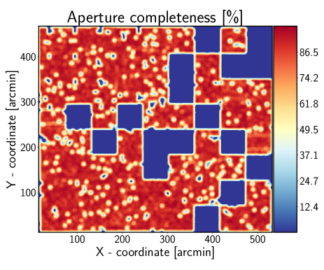
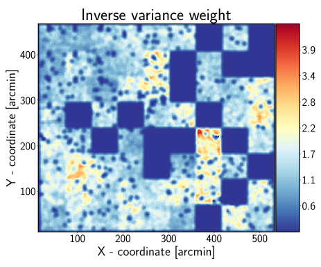
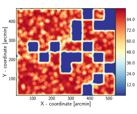
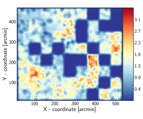
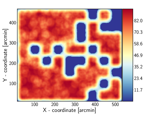
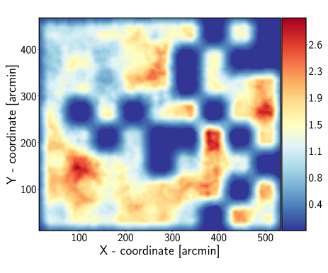
Figure 4: Same as Figure 3, but this time columns indicate aperture completeness (left) and the aperture weights derived from Eq. (53), using the shot noise dominated limit of Eq. (42) (right). The weight maps shown are rescaled by their inverse mean. As expected, the weight depends on the local galaxy number density and on the aperture completeness.

Table 1: Overview of the CFHTLenS data.

Field	$\#$ of galaxies	Angular Area $\Omega_{s}\ [{\rm deg}]^{2}$	$\bar{n}\ [{\rm arcmin}]^{-2}$
W1	1871709	42.36	12.27
W2	499372	11.72	11.84
W3	1192084	25.23	13.12
W4	558515	12.55	12.36

In this work we make use of the final public data release. The combined data set of W1, W2, W3 and W4 contains ellipticity measurements for 4,121,680 galaxies. In Table 1 we provide a summary overview of the data. Associated with each galaxy are: the angular positions RA and DEC, in radians; the $x$- and $y$-pixel coordinates in the projected tangent map; the ellipticity estimates $\epsilon_{1}$ and $\epsilon_{2}$, the lens weights $w$; the shear bias correction $c$ and the multiplicative bias correction $m$; photometric redshift estimate $z_{\rm phot}$. Figure 1 shows the redshift distribution and lensing efficiency for the sources in each of the four CFHTLenS fields.

Table 2: zHORIZON  cosmological parameters. Columns are (from left to right): density parameters for matter, dark energy and baryons; the amplitude of the power spectrum; the dark energy equation of state parameters; the spectral index of the primordial power spectrum; the Hubble parameter.

Cosmological model	$\Omega_{\rm m,0}$	$\Omega_{\rm DE,0}$	$\Omega_{\rm b,0}$	$\sigma_{8}$	$w_{0}$	$w_{a}$	$n_{s}$	$h$
Fiducial	0.25	0.75	0.04	0.8	-1	0	1	0.7
$\Omega_{\rm m,0}^{\pm}$	0.2/0.3	0.8/0.7	0.04	0.8	-1	0	1	0.7
$\Omega_{\rm b,0}^{\pm}$	0.25	0.75	0.035/0.45	0.8	-1	0	1	0.7
$\sigma_{8}^{\pm}$	0.25	0.75	0.04	0.7/0.9	-1	0	1	0.7
$w_{0}^{\pm}$	0.25	0.75	0.04	0.8	-1.2/-0.8	0	1	0.7
$w_{a}^{\pm}$	0.25	0.75	0.04	0.8	-1	-0.2/0.2	1	0.7
$n_{s}^{\pm}$	0.25	0.75	0.04	0.8	-1	0	0.95/1.05	0.7
$h^{\pm}$	0.25	0.75	0.04	0.8	-1	0	1	0.65/0.75

5.2 Simulating the CFHTLenS data

In order to understand the statistical properties of the data we have generated a large set of simulated CFHTLenS skies. These mock data were generated from ray-tracing through $N$-body simulations. We used the zHORIZON simulations, performed on the zBOX-2 and zBOX-3 supercomputers at the University of Zürich, described in detail in Smith (2009). Each of the zHORIZON simulations was performed using the publicly available Gadget-2 code (Springel, 2005), and followed the nonlinear evolution under gravity of $N=750^{3}$ equal-mass particles in a comoving cube of length $L_{\rm sim}=1500\,h^{-1}{\rm Mpc}$; the softening length was $l_{\rm soft}=60\,\,h^{-1}{\rm kpc}$. For all realizations 11 snapshots were output between redshifts $z=[0,2]$; further snapshots were at redshifts $z=\{3,4,5\}$. The transfer function for the simulations was generated using the publicly available cmbfast code (Seljak & Zaldarriaga, 1996), with high sampling of the spatial frequencies on large scales. Initial conditions were set at redshift $z=50$ using the serial version of the publicly available 2LPT code (Scoccimarro, 1998; Crocce, Pueblas & Scoccimarro, 2006). The simulations correspond to several cosmological models, with parameters varying around a fiducial model. The latter closely matched the results of the WMAP experiment (Komatsu et al., 2009). There are 8 simulations of the fiducial model, and 4 of each variational model, matching the random realization of the initial Gaussian field with the corresponding one from the fiducial model. Table 2 summarizes the cosmological parameters that we simulated.

From each zHORIZON simulation, 16 large fields of view were generated by choosing different observer positions within the simulation box. These large fields have side lengths of $12\,\mathrm{deg}$ and are covered by a regular mesh of $4096^{2}$ pixels. For each pixel, a light ray was traced back through the simulation by a multiple-lens-plane algorithm (see Hilbert, Metcalf & White, 2007; Hilbert et al., 2009), and its distortion due to gravitational lensing was recorded for a set of $45$ source redshifts between 0 and 4.

Each of the large fields was used to create four simulated mock-CFHTLenS wide field source galaxy catalogues for each of the different CFHTLenS fields W1 to W4 (i.e., 64 mock catalogues per CFHTLenS field and zHORIZON simulation). The basis for the simulated source galaxy catalogues are the actual CFHTLenS source catalogues, from which the angular positions and redshifts were taken. The reduced shear $g\equiv\gamma/(1-\kappa)$ for each galaxy in the mock catalogues was computed by multi-linear interpolation of the simulated lensing distortions onto the source galaxy’s angular position and redshift (using a different angular offset within the $12\times 12\,\mathrm{deg}^{2}$ simulated fields for each mock catalogue). The ‘observed’ source galaxy ellipticities in the simulated catalogues were then computed by combining the reduced shear from the ray-tracing and the randomly rotated observed ellipticities from the actual source galaxy catalogue.

5.3 Maps from the CFHTLenS data

As a first step in our analysis of the CFHTLenS data, we compute several aperture based maps for the four fields of the CFHTLenS. To generate these maps the survey area was pixelated and the corresponding maps were computed for apertures located at the pixel centers. We furthermore only include apertures that are at least $20$ per cent complete, the map values for all less complete apertures are set to the minimum value and therefore appear as blue pixels. Images of the official CFHTLenS masks are presented in Appendix B.

In Figure 3 we show the aperture mass map and its corresponding signal-to-noise map for the W1 field. The aperture masses are estimated using Eq. (44) while the noise for each aperture was estimated as (Hetterscheidt, M. et al., 2005):

$$\widehat{\sigma^{2}\left(\mathcal{M}_{\mathrm{a}p}({\bm{\theta}}_{0}|{\vartheta})\right)}=\frac{(\pi{\vartheta}^{2})^{2}\sum_{i}w_{i}^{2}Q_{i}^{2}\epsilon_{{\rm t},i}^{2}}{2\left(\sum_{i}w_{i}\right)^{2}}\ .$$ (56)

The results are shown for the Schneider filter Eq. (11) with aperture extent in the set ${\vartheta}\ \in\ [5^{\prime},\ 10^{\prime},\ 20^{\prime}]$. It is interesting to note that near the survey mask boundaries the value of the aperture mass obtains large positive and negative values. This is due to the fact that for incomplete apertures the ring averaged tangential shear becomes biased as the mask induces non-vanishing $B$-modes (cross-shear). How to deal with the effects of masked apertures will be discussed in detail below and in a companion paper.

In Figure 4 we show the aperture completeness map as well as a map of the aperture weights derived from Eq. (53), using the shot noise dominated limit of Eq. (42). We rescaled the latter map by its inverse mean such that the mean weight becomes unity. From there we can explicitly see that such aperture weights depend on the aperture completeness, cosmic structures and on the local depth of the survey. Analogous maps for the other three fields are presented in Appendix C.

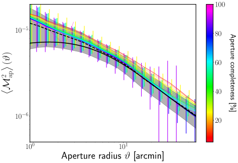
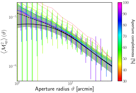
Figure 5: Left panel: Aperture mass variance as a function of aperture radius computed from the 512 full-ray traced CFHTLenS mock catalogues of the fiducial runs of the W1 field for the different weighting schemes described in the text. The thick solid line gives the theoretical prediction evaluated via Eq. (20). The thin solid lines show results from the direct approach where the estimates from each apertures are combined with equal weight (this is Eq. (51) in the text). The colour of the lines indicates the value of the aperture completeness parameter $c_{k}=A_{k}/A$ – only apertures with a completeness greater than this value are used in the estimate. The thick dashed line gives the result from the correlation function approach as obtained using the TreeCorr routine (Jarvis, Bernstein & Jain, 2004). The error bars show the error for a single realisation of the CFHTLenS W1 field. The grey shaded region are for TreeCorr . Note that the errors from the direct estimator approach have been slightly offset for clarity. Right panel: shows the same as the left panel, except this time the estimates from the direct estimator have been computed in bins of aperture completeness. The diffenence between the simulations and the theoretical predictions for small aperture radii can be attributed to shot noise and the line-of-sight discretization from which the simulated data suffers (Hilbert et al., 2020).

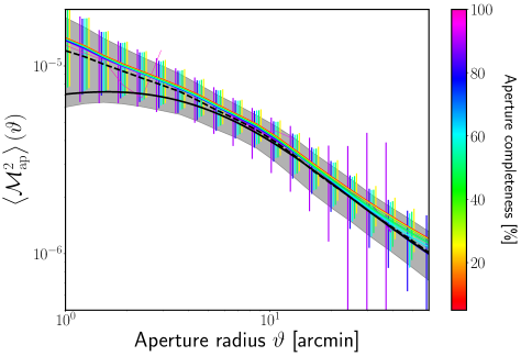
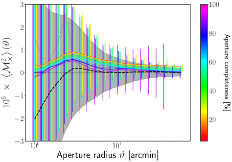
Figure 6: Left panel: Same as Figure 5, however this time the estimates for each aperture are combined using an inverse variance weighting scheme (this is Eq. (53) in the text). Note that when $c_{k}\lesssim 10\%$ is equivalent to the case where all apertures are considered irrespective of coverage and their results are combined using an inverse variance weight. Right Panel: Same as the left panel, but this time showing the variance of the cross component of aperture mass. As shown in Eq. (54) and in the absence of systematic errors, $\left<{\mathcal{M}}_{\times}^{2}({\vartheta})\right>=0$.

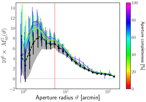
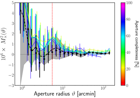
Figure 7: Left panel: Aperture mass variance as a function of aperture cut-off scale as measured in the CFHTLenS data. The results for the direct estimator are indicated as coloured lines, where the line colour indicates the value of aperture completeness that was used. The thick dashed line gives the result from the correlation function approach as obtained using the TreeCorr routine (Jarvis, Bernstein & Jain, 2004). The error bars show the error for the full CFHTLenS. Right panel: Same as the left panel, but for the variance of the cross component of the aperture mass.

6 Measurements of the aperture mass variance

We now turn to the estimation of the aperture mass variance from the CFHTLenS data using the direct and correlation function estimators.

6.1 Analysis of the CFHTLenS mock skies

Before performing our statistical analysis of the real CFHTLenS data we first make a study of the direct and correlation function estimators as applied to the mocks. From this we will be able to determine whether the methods are consistent with one another to within the errors and also which of the three weighting schemes given by Eqs. (51) and (53) provides the better method for estimating $\left<{\mathcal{M}}_{\rm ap}^{2}\right>({\vartheta})$.

The left panel of Figure 5 shows the variance of the aperture mass estimated from the mocks, as a function of the aperture radius. For the results presented in this section we used a spacing of $d=0.25\ \vartheta$ between the apertures. The thin coloured lines show the results from the direct estimator approach where the estimates from individual apertures are combined with equal weight, but where a completeness thresholds $c_{k}$ has been adopted – this is equivalent to weight scheme ${\mathcal{W}}_{1}$ c.f. Eq. (51). For example the magenta lines show a conservative case, where only apertures with completeness $c_{k}\gtrsim 90\%$ are taken, whereas the red lines are the most relaxed where all apertures with $c_{k}\gtrsim 10\%$ are allowed. The thick dashed line shows the results obtained from the correlation function method, where the pair counts have been measured using the TreeCorr code of Jarvis, Bernstein & Jain (2004). The grey shaded regions shows the standard error for the correlation function method and the error bars are the errors on direct estimator. In all cases these were determined from the ensemble of 512 mocks of our fiducial model. The right panel of Figure 5 shows the same as the left panel, however the results from the direct estimator have been binned in completeness. Both panels also show the theoretical prediction evaluated via Eq. (20).

The figure shows that there is a clear bias in the direct estimator approach when the apertures have a low completeness. This is manifest as an increased amplitude of the signal on all scales. However, for apertures with $c_{k}\gtrsim 75\%$ completeness (blue line) we find that the results are in good agreement with the case of $c_{k}\gtrsim 90\%$ (magenta line) and that these are fully consistent with the correlation function results on large scales, to within the errors. We note that on scales smaller than $\sim 5^{\prime}$ the results from TreeCorr appear to be biased slightly low to those from the direct estimator approach. We furthermore note a difference between the theoretical prediction and the measurements for small aperture radii which is due to shot noise and the line-of-sight discretization from which the simulated data suffers (Hilbert et al., 2020).

The left panel of Figure 6 again shows the aperture mass variance estimated from the mocks for the two methods, but this time the estimates from individual apertures are combined using the inverse variance weighting schemes with a completeness threshold – that is we now employ ${\mathcal{W}}_{2}$ and ${\mathcal{W}}_{3}$, c.f. Eqs. (52) and (53). The right panel of Figure 6 shows the variance of the cross component of the aperture mass $\left<{\mathcal{M}}_{\times}^{2}\right>({\vartheta})$ from Eq. (54), which for B-mode free fields should vanish.

There are a number of interesting points to note from this analysis. First, we see that all of the estimates from the direct estimator are consistent with one another and that they all lie within the error bars of the TreeCorr result. Nevertheless, for scales ${\vartheta}>20^{\prime}$ we still observe that the direct estimator approach appears to be slightly biased high on large scales for aperture completeness values $c_{k}\gtrsim 40\%$ compared to the correlation function method. However, for aperture completeness levels $c_{k}\gtrsim 75\%$ we see excellent agreement between the two methods. On small scales, ${\vartheta}<5^{\prime}$, the correlation function method gives slightly lower results than the direct estimator. Here we believe that the direct estimator is correct, since as was noted in Kilbinger, Schneider & Eifler (2006), the correlation function method is biased low on scales of the order ${\vartheta}\sim 1^{\prime}$ due to the absence of correlation function bins on small scales. In the TreeCorr code the small-scale cutoff in the pair counts is set at ${\vartheta}>6^{\prime\prime}$. Note that in the mock data there is no image blending and so the direct estimator should not suffer from this suppression. For the observed CFHTLenS data this is not necessarily the case.

We also note that, as shown in the right panel of Figure 6, the cross component of the aperture mass variance is consistent with zero to within the error bars for all completeness fractions used. However, the $c_{k}\gtrsim 40\%$ shows a small positive offset from zero at the level of below $5\times 10^{-7}$. On large and small scales the bias is very small for $c_{k}\gtrsim 75\%$. This gives us further confidence that the discrepancy between the direct estimator and TreeCorr on small scales is due to the bias in the correlation function approach.

Another point of interest, is that we see the error bars on the most conservative completeness cuts, $c_{k}\gtrsim 95\%$, are significantly larger than those obtained from the correlation function method. This makes sense, since, for the case of the most conservative cuts, one can find only a few apertures that meet the criterion. On the other hand, for completeness fractions of the order $c_{k}\gtrsim 70\%$, the error bars between the two methods are comparable.

Based on the discussion above, we will be using the weighting scheme ${\mathcal{W}}_{3}$ for the analysis of the observed CFHTLenS data.

6.2 Calibration of the estimators for ellipticity bias

We now turn to the analysis of the observed data. As discussed in §4 the aperture mass variance for a set of apertures can be directly estimated using Eqs. (47) and (33). However, owing to calibration errors in the lensfit shape estimation algorithm (Miller et al., 2013), each galaxies ellipticity has a corresponding multiplicative $m$ and additive $c$ bias. Hence, the observed and true ellipticity components of the $i$th galaxy are related through:

$$\epsilon_{1,i}^{\rm obs} =(1+m_{i})\epsilon_{1,i}^{\rm true}+c_{1,i}\ ;$$ (57)

$$\epsilon_{2,i}^{\rm obs} =(1+m_{i})\epsilon_{2,i}^{\rm true}+c_{2,i}\ .$$ (58)

For the CFHTLenS $c_{1}$ was found to be consistent with zero, however $c_{2}$ was found to have a $S/N$ and size dependent bias that was subtracted from each galaxy. On average this correction was of the order $2\times 10^{-3}$.

Correction for shear correlation functions: following Miller et al. (2013), the shear correlation functions can be corrected for multiplicative bias through the following procedure. The ’raw’ shear correlation functions are first estimated from the ‘observed’ shears using the estimator:

$$\widehat{\xi^{\rm raw}_{\pm}}(\theta_{\alpha})=\frac{\sum_{i}\sum_{j\neq i}w_{i}w_{j}\left[\epsilon^{\rm obs}_{{\rm t},i}\epsilon^{\rm obs}_{{\rm t},j}\pm\epsilon^{\rm obs}_{\times,i}\epsilon^{\rm obs}_{\times,j}\right]\Pi(\theta_{ij}|\theta_{\alpha})}{\sum_{i}\sum_{j\neq i}w_{i}w_{j}\Pi(\theta_{ij}|\theta_{\alpha})}\ ,$$ (59)

where $\theta_{ij}\equiv|{\bm{\theta}}_{i}-{\bm{\theta}}_{j}|$ and where $\Pi(\theta_{ij}|\theta_{\alpha})$ is the pair binning function which is unity if $\theta_{ij}$ lies in the range $[\theta_{\alpha}-\Delta\theta/2,\theta_{\alpha}+\Delta\theta/2)$. If we now insert Eqs. (57) and (58) into the above estimator (taking $c_{1,i}=0$ and $c_{2,i}=0$) we find:

$$\widehat{\xi^{\rm raw}_{\pm}(\theta_{\alpha})}=\frac{\sum_{j\neq i}w_{i}^{\prime}w_{j}^{\prime}\left[\epsilon^{\rm true}_{{\rm t},i}\epsilon^{\rm true}_{{\rm t},j}\pm\epsilon^{\rm true}_{\times,i}\epsilon^{\rm true}_{\times,j}\right]\Pi(\theta_{ij}|\theta_{\alpha})}{\sum_{j\neq i}w_{i}w_{j}\Pi(\theta_{ij}|\theta_{\alpha})}\ ,$$ (60)

where in the above we introduced the new weights $w_{i}^{\prime}\equiv w_{i}(1+m_{i})$, then we see that the above equation can be rewritten:

$$\widehat{\xi^{\rm raw}_{\pm}(\theta_{\alpha})} =\left(\frac{\sum_{j\neq i}w^{\prime}_{i}w^{\prime}_{j}\left[\epsilon^{\rm true}_{{\rm t},i}\epsilon^{\rm true}_{{\rm t},j}\pm\epsilon^{\rm true}_{\times,i}\epsilon^{\rm true}_{\times,j}\right]\Pi(\theta_{ij}|\theta_{\alpha})}{\sum_{j\neq i}w_{i}^{\prime}w_{j}^{\prime}\Pi(\theta_{ij}|\theta_{\alpha})}\right)$$

$$\times\left(\frac{\sum_{j\neq i}w_{i}^{\prime}w_{j}^{\prime}\Pi(\theta_{ij}|\theta_{\alpha})}{\sum_{j\neq i}w_{i}w_{j}\Pi(\theta_{ij}|\theta_{\alpha})}\right)\ ,$$ (61)

The first term on the right in parenthesis is the ‘calibrated’ true shear correlation which we can write as $\xi^{\rm cal}_{\pm}$, hence we can write:

$$\widehat{\xi^{\rm cal}_{\pm}(\theta_{\alpha})}=\frac{\xi^{\rm raw}_{\pm}(\theta_{\alpha})}{1+{\mathcal{K}}(\theta_{\alpha})}\ \ ;\ \ 1+{\mathcal{K}}(\theta_{\alpha})\equiv\frac{\sum_{j\neq i}w_{i}^{\prime}w_{j}^{\prime}\Pi(\theta_{ij}|\theta_{\alpha})}{\sum_{j\neq i}w_{i}w_{j}\Pi(\theta_{ij}|\theta_{\alpha})}\ .$$ (62)

Correction for direct aperture mass variance estimator: following in the footsteps of the shear correlation function approach, we define the raw uncorrected aperture mass variance estimate as:

$$\left[\widehat{{\mathcal{M}}_{\rm ap}^{2}({\vartheta}|\mn@boldsymbol{\theta}_{0,k})}\right]^{\rm raw} =(\pi{\vartheta}^{2})^{2}\ \frac{\sum_{j\neq i}w_{i}\ w_{j}\ Q_{i}\ Q_{j}\ \epsilon^{\rm obs}_{{\rm t},i}\ \epsilon^{\rm obs}_{{\rm t},j}}{\sum_{j\neq i}w_{i}w_{j}}\ ,$$ (63)

recalling that the sums only extend over the galaxies in the aperture. If we now insert Eqs. (57) and (58) into the above estimator, as before, then we find:

$$\left[\widehat{{\mathcal{M}}_{\rm ap}^{2}({\vartheta}|\mn@boldsymbol{\theta}_{0,k})}\right]^{\rm raw} =(\pi{\vartheta}^{2})^{2}\ \frac{\sum_{j\neq i}w_{i}^{\prime}\ w_{j}^{\prime}\ Q_{i}\ Q_{j}\ \epsilon^{\rm true}_{{\rm t},i}\ \epsilon^{\rm true}_{t,j}}{\sum_{j\neq i}w_{i}w_{j}}\ .$$ (64)

Again, on redefining the lensfit weights this leads us to write:

$$\left[\widehat{{\mathcal{M}}_{\rm ap}^{2}({\vartheta}|\mn@boldsymbol{\theta}_{0,k})}\right]^{\rm raw} =\left((\pi{\vartheta}^{2})^{2}\frac{\sum_{j\neq i}w_{i}^{\prime}\ w_{j}^{\prime}\ Q_{i}\ Q_{j}\ \epsilon^{\rm true}_{{\rm t},i}\ \epsilon^{\rm true}_{{\rm t},j}}{\sum_{j\neq i}w_{i}^{\prime}w_{j}^{\prime}}\right)$$

$$\times\left(\frac{\sum_{j\neq i}w_{i}^{\prime}w_{j}^{\prime}}{\sum_{j\neq i}w_{i}w_{j}}\right)\ .$$ (65)

Thus we see that the calibrated estimate of the aperture mass variance can be written:

$$\left[\widehat{{\mathcal{M}}_{\rm ap}^{2}({\vartheta}|\mn@boldsymbol{\theta}_{0,k})}\right]^{\rm cal}=\frac{\left[\widehat{{\mathcal{M}}_{\rm ap}^{2}({\vartheta}|\mn@boldsymbol{\theta}_{0,k})}\right]^{\rm raw}}{1+{\mathcal{K}}^{\rm ap}({\vartheta}|\mn@boldsymbol{\theta}_{0,k})}\ ,$$ (66)

where the normalisation factor is

$$1+{\mathcal{K}}^{\rm ap}({\vartheta}|\mn@boldsymbol{\theta}_{0,k})\equiv\frac{\sum_{j\neq i}w_{i}w_{j}(1+m_{i})(1+m_{j})}{\sum_{j\neq i}w_{i}w_{j}}\ .$$ (67)

6.3 Analysis of the CFHTLenS data

In left panel of Figure 7 we show the aperture mass variance and in the right the variance of the cross component variance, estimated from the CFHTLenS. The results shown are for the full combination of the W1, W2, W3 and W4 survey areas. For the direct aperture mass variance approach the estimate was obtained using the weighting scheme ${\mathcal{W}}_{3}$, c.f. Eq. (53), and the error was obtained using a weighted jackknife resampling of the data in patches having an area of roughly $(1\ \mathrm{deg})^{2}$. For the method of measuring the aperture mass variance from the shear correlation functions (thick, black dashed line), when combining the results from each field, we have simply weighted the estimates in proportion to the field area.

In Fig. 7 the vertical dashed line indicates the scale ${\vartheta}=5.5^{\prime}$ identified in Kilbinger et al. (2013), above which the E/B-mode leakage is claimed to be $\lesssim 1.5\%$. The E/B mode leakage on smaller scales originates from the $9^{\prime\prime}$ cut-off in the shear-correlation functions, which originates from the blending of galaxy images and a shear bias for close pairs (see §6.4).

The important point to note from the figure is that on scales ${\vartheta}>5.5^{\prime}$ the measurements from the direct and correlation function estimators are in very good agreement to within the errors for a wide range of aperture completeness thresholds. In addition, with the exception of all but the lowest $c_{k}$ thresholds, the variance of the cross component of the aperture mass variance is consistent with zero on the same scales. On scales ${\vartheta}\leq 5.5^{\prime}$, both estimators appear to have non-zero B-modes, which rise sharply on scales ${\vartheta}\lesssim 2^{\prime}$.

6.4 Impact of close pair image blending on the variance

As noted in Miller et al. (2013), lensfit galaxies with separations closer than $9^{\prime\prime}$ tend to have a bias in their ellipticities which is in the direction of the line connecting the centres of the galaxy images. For the shear correlation functions, Kilbinger et al. (2013) stated that this bias can be removed by only computing the shear correlation functions down to $9^{\prime\prime}$. Their justification was that the alignment direction of the pair is, to a very good approximation, randomly orientated. We now investigate how such a bias may contaminate the direct estimator approach for aperture mass variance by comparing the measurements of the full catalogue to a reduced one in which clustered galaxies below the blending scale are removed.

We proceed by describing our algorithm for removing close pairs of galaxies to generate a reduced catalogue.

1. We begin by initializing a Boolean mask value for each galaxy. These values are all initially set to unity.

2. We then spatially organize the data using a hierarchical KD-tree.

3. We next set the pair-cut-off scale $\theta_{\rm pc}$, within which galaxy pairs are to be expunged from the catalogue.

4. We now loop over all galaxies and perform a range search. If any of the galaxy positions lie within the sphere of radius $\theta_{\rm pc}$ and have their Boolean flag set to unity, then the Boolean mask value associated with the current galaxy is set to zero and the galaxy will henceforth be excluded when estimating statistics from the data.

We apply this method to the CFHTLenS data and set the pair-cut-off scale $\theta_{\rm pc}=9^{\prime\prime}$. This yields a reduced catalogue that contains $\sim$70% of the original galaxies.

Figure 8 shows the probability density function of the distance to the nearest-neighbour galaxy. Note that these curves have been normalised so that the area under the graph gives unity.

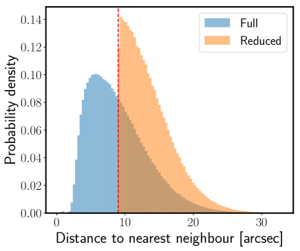
Figure 8: The probability density functions of the nearest neighbour distances in the CFHTLenS. The blue histogram shows the distribution before applying our exclusion algorithm and the orange one shows the result after setting the pair-cut-off scale $\theta_{\rm pc}=9^{\prime\prime}$. The vertical dashed red line indicates $\theta_{\rm pc}$.

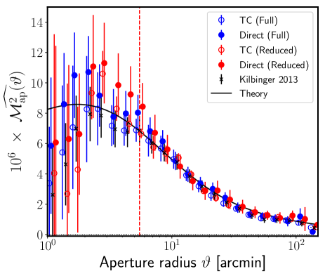
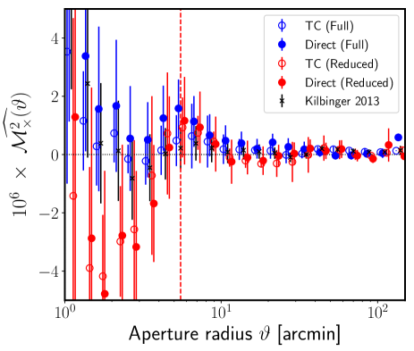
Figure 9: (Left panel): Comparison of the aperture mass variance from the full and small scale-pair reduced CFHTLenS catalogues. The open circles show the results from TreeCorr and the solid points the results from the direct estimator when including all apertures with $c_{k}>0.7$. The red and blue colours indicate the full and reduced catalogues, respectively. The black crosses and the black line show the published measurements from Kilbinger et al. (2013) and the corresponding theoretical prediction for their best-fit cosmology evaluated via Eq. (20). The vertical red dashed line indicates the scale above which the E/B mode leakage should be less than 1% for the correlation function method. (Right panel): same as left panel, except this time for the cross component of the aperture mass variance.

Figure 9 shows our measurements of the aperture mass variance and the variance of the cross component of aperture mass, in the full and the close-pair reduced CFHTLenS shear catalogues. We compare the results from both the direct and the correlation function estimators. For the direct estimator approach we have employed the weighting function ${\mathcal{W}}_{3}$, with the completeness threshold set to $c_{k}=0.7$. Some important points can be noted: looking at the left panel of Fig. 9 the result of excluding pairs of galaxies that are closer then 9” lowers the amplitude of ${\left<{\mathcal{M}}_{\rm ap}^{2}\right>}$ by less than $15\%$ for small aperture scales ($\sim 10^{\prime}$). For larger apertures the changes are smaller. Interestingly, the results from the TreeCorr analysis of the full and reduced catalogue also show similar differences: for small aperture scales, the aperture mass variance appears to be lower in the reduced catalogue. In addition, we see that all of the estimators agree to within the errors on all scales. However, the agreement between the direct estimator and the TreeCorr result is exceptionally good for the measurements from the reduced catalogue.

It is also interesting to compare these results with the published measurement from Kilbinger et al. (2013) (denoted as the black crosses in the plot). Here we see that our measurements are fully consistent with the Kilbinger et al. (2013) measurements, to within the errors. The right panel of Figure 9 shows that the variance of the cross-component of the aperture mass is reassuringly consistent with zero for both estimators applied to both the full and reduced catalogues.

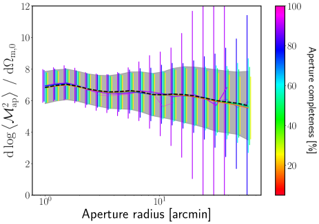
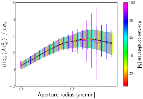
Figure 10: Estimates of the derivatives of the aperture mass variance with respect to the cosmological parameters. The left and right panels show the results for the variations with respect to the matter density parameter $\Omega_{\rm m,0}$ and the variance of matter fluctuations $\sigma_{8}$, respectively. The solid lines all show the results measured from the direct estimator approach, where the colour of the line indicates the value for the aperture completeness parameter that was adopted. The error bars indicate the errors in the ensemble. The black dashed line shows the results from the correlation function approach as measured using TreeCorr . The shaded region shows the standard error on the TreeCorr estimates.

7 Information content of the estimators

We now turn our attention to the question of addressing the possible information loss in using the direct estimator approach. We will do this using the Fisher matrix formalism. If we assume that the likelihood function for measuring the aperture mass variance for a set of $N_{d}$ aperture scales is Gaussian, and that the priors on the cosmological parameters are flat, then the Fisher information matrix can be written (Tegmark, Taylor & Heavens, 1997):

$${\mathcal{F}}_{\alpha\beta}=\frac{1}{2}{\rm Tr}\left[\textbf{{C}}^{-1}\frac{\partial\textbf{{C}}}{\partial p_{\alpha}}\textbf{{C}}^{-1}\frac{\partial\textbf{{C}}}{\partial p_{\beta}}\right]+\frac{\partial\bm{\mu}^{\rm T}}{\partial p_{\alpha}}\textbf{{C}}^{-1}\frac{\partial\bm{\mu}}{\partial p_{\beta}}\ ,$$ (68)

where $\bm{\mu}^{\rm T}=\left(\widehat{\mathcal{M}^{2}_{\rm ap}({\vartheta}_{1})},\dots,\widehat{\mathcal{M}^{2}_{\rm ap}({\vartheta}_{N_{d}})}\right)$ is the set of model means measured at the bin centres and C is the model covariance matrix. The vector ${\bm{p}}$ is the set of cosmological parameters. In this study we will restrict our attention to the cosmological parameters $\sigma_{8}$ and $\Omega_{\rm m,0}$, as these are the most readily constrained from lensing data. The minimum variance bounds on a given cosmological parameter, after marginalising over all other parameters, can be obtained as:

$$\sigma^{2}_{p_{\alpha}}=\left[{\mathcal{F}}^{-1}\right]_{\alpha\alpha}\ .$$ (69)

In order to simplify the calculation, we will assume that the first term on the right-hand-side of Eq. (68) is significantly smaller than the other term. As was noted in §6 of Smith & Marian (2015) this can be justified in the high-$k$ limit through mode counting arguments, however, it is in general an incorrect assumption.

In order to compute the second term of Eq. (68) we follow the approach lain down in Smith et al. (2014) and use the mocks to evaluate all quantities. That is we measure the derivatives of the model mean with respect to the cosmological parameters and we also estimate the precision matrix $\textbf{{C}}^{-1}$. To do these tasks we make use of the ray traced mock CFHTLenS data. The derivatives are estimated using:

$$\widehat{\frac{\partial\mu_{i}}{\partial p_{\alpha}}}=\sum_{j=1}^{N_{\rm ens}}\frac{\widehat{{\mathcal{M}}_{\rm ap,{(j)}}^{2}}({\vartheta}_{i}|p_{\alpha}+\Delta p_{\alpha})-\widehat{{\mathcal{M}}_{\rm ap,{(j)}}^{2}}({\vartheta}_{i}|p_{\alpha}-\Delta p_{\alpha})}{2N_{\rm ens}\Delta p_{\alpha}}\ ,$$ (70)

where $N_{\rm ens}$ is the number of realisation of the ensemble, and ${\mathcal{M}}_{\rm ap,{(j)}}^{2}(\theta_{i}|p_{\alpha}+\Delta p_{\alpha})$ is the estimate of the aperture mass variance on scale $\theta_{i}$ in the $j$th realisation of the mocks, for the simulation with cosmological parameters $p_{\alpha}+\Delta p_{\alpha}$. In computing Eq. (70) we use the 256 mock ray-tracing simulations of each cosmological variation of the CFHTLenS data. Note that the above estimator will reduce the cosmic variance, since when running the modified cosmology simulations we used Fourier phase realisations that were identical to the fiducial model runs. In addition, when estimating the precision matrix we take account of the bias in the estimator using the method described in Hartlap, Simon & Schneider (2007):

$$\widehat{\textbf{{C}}^{-1}}=\frac{N_{\rm ens}-N_{\mathrm{d}}-2}{N_{\rm ens}-1}\left[\widehat{\textbf{{C}}}\right]^{-1}\ ,$$ (71)

where $N_{\mathrm{d}}$ is the dimension of the data vector and $\widehat{\textbf{{C}}}$ is the standard maximum likelihood estimator of the covariance matrix of the data.

Figure 10 shows the derivatives of the aperture mass variance with respect to the cosmological parameters, estimated from the 256 ray-traced mock simulations. The agreement between the results from the direct estimator approach is excellent, for all of the $c_{k}$ values that we considered, where we used the inverse variance weighting approach of ${\mathcal{W}}_{3}$ to combine estimates from individual apertures. In addition, these also agree with the results from the correlation function approach to a high degree of accuracy. The only issue to note is that for high completeness fractions $c_{k}\sim 1$ the estimates become very noisy.

Figure 11: Top left and bottom right panels show the 1D posterior distributions, marginalised over all other parameters, for $\Omega_{\rm m,0}$ and $\sigma_{8}$, respectively. The bottom left panel shows the 2D confidence interval ellipse for the joint posterior distribution of $\Omega_{\rm m,0}$ and $\sigma_{8}$. The coloured lines again show the results from the Fisherm matrix forecast using the direct estimator approach for various aperture completeness thresholds $c_{k}$. The dashed line shows the results from TreeCorr .

Figure 11 shows the 2D confidence contour for $\Omega_{\rm m,0}$ and $\sigma_{8}$, and also the 1D posterior distributions, marginalised over all other parameters, for the same two parameters. Focusing on the 2D contours, we notice a number of interesting points: first, considering the results for the direct estimator, we see that as we decrease the threshold completeness value $c_{k}$, the ellipses rotate clockwise by a small amount. This difference in orientation can be explained by noting that for a CFHTLenS like survey the off-diagonal elements of the covariance matrix are getting more and more noisy for increasing values of $c_{k}$. The reason for this is that the effective survey footprint changes for different aperture radii and that this difference is most prominent for conservative aperture completeness cuts. When choosing a $c_{k}$ of around $0.7$ or lower, the covariance matrices become stable and so does the orientation and area of the ellipse.

Similar observations can be made for the 1D marginalized posterior distributions which lets us conclude that, within the Fisher Matrix formalism, the information content of the direct estimator is comparable with the correlation function method.

There are some caveats that must be mentioned to the interpretation of these results. Firstly, both the precision matrix and the model means are estimated from the mock simulations of the CFHTLenS, and are therefore subject to errors. This means that the forecasted constraining power should also come with an error. Since we are only interested in the relative information, we have not taken this into account. A more detailed study is required in order to make a more precise statement, and this is beyond the scope of this work.

8 Conclusions and discussion

In this paper we have explored an alternative method for estimating the aperture mass statistics in weak lensing cosmic shear surveys. Our method is a direct estimator of the variance. With the use of a hierarchical KD-tree algorithm for ordering the data we found that the computational time for execution of this estimator was linear in the number of galaxies per aperture and the number of apertures used in the estimate. This paper, the first in a series, focused on the two-point statistics, and in particular the aperture mass variance. The summary is:

In §2 and §3 we reviewed the background theory of weak lensing in the cosmological context and the aperture mass variance and its connection to the matter power spectrum. Here we also discussed the standard approach for estimating this quantity, which relies on measurements of the shear correlation functions.

In §3 we introduce the direct estimator for the aperture mass variance that we employ. We show that when including ellipticity weights the estimator is unbiased. We also compute the variance of the estimator and show that in the limit of Gaussian shear signal, no source clustering and a large number of galaxies per aperture that the variance reduces to a simple expression. We then show how the original estimator introduced by Schneider et al. (1998) can be accelerated to linear order in the number of galaxies per aperture. We also discuss various weighting schemes for combining the estimates from different apertures. Finally, we illuminate the computational complexity of our estimator.

In §4 we give an overview of the CFHTLenS data and we also describe our method for generating mocks of the survey using full gravitational ray-tracing simulations through $N$-body simulations. As a first test, we measured the aperture mass maps from the survey data.

In §6 we computed the aperture mass variance from our mock surveys, using both the direct estimator and correlation function method. We found that if we included incomplete apertures in the direct estimate method, and if we combined all apertures equally that there was a significant bias in the final result. This bias vanished if only complete apertures were used. However, the errors on the estimates increased significantly. We then explored an alternative weighting scheme, where the apertures were combined using an inverse variance weighting approach, where the variance was assumed to be dominated by shape noise. The results in this case were found to be in excellent agreement with the alternative method, even in the case where incomplete apertures were included in the estimate. We found that an aperture completeness threshold of $\sim 0.7$ gave very good results and contained only a small residual of B-modes, that were contained well within the error tolerance.

We then turned to the application of the method to the CFHTLenS data. It was necessary to account for two additional observational biases: first, we derived the correction factors required to account for the ellipticity bias in our estimator; second, we created a modified source galaxy catalogue that removed pairs of galaxies whose images were in close projection on the sky whose ellipticities are biased by an artefact in the ellipticity estimator algorithm lensfit. On taking account of these we found that our direct estimator approach and our estimates using the shear correlation function were in excellent agreement with the published data from Kilbinger et al. (2013).

In §7 we explored the information content of the direct estimator approach and compared it with that from the correlation function method. We found that the 1D marginalised posterior distributions for $\sigma_{8}$ were less constraining for high aperture completeness than the shear correlation function method, but that as some incomplete apertures were included in the estimate the distributions became very similar. This trend was mirrored for $\Omega_{\rm m,0}$, except that for high completeness the distribution for the direct estimator was the most constraining. This may be due to errors in the forecast due to uncertainties in the precision matrix and derivatives. The 2D confidence contours for $\Omega_{\rm m,0}$ and $\sigma_{8}$ were roughly the same size for all aperture completeness thresholds, however they rotated to be in the same direction as those of the correlation function approach as lower thresholds were taken. This leads us to conclude, at this stage, that the information content of the two estimators is comparable.

The main advantage of this development in not to replace the correlation function approach as the way to measure aperture mass statistics and other associated statistics, but to show that it is a credible method. As mentioned earlier, the real advantage of this approach is that it can be easily generalised to enable the measurement of higher order aperture mass statistics such as the skewness and kurtosis with very little extra effort. While these can of course also be estimated using the shear three-point and four-point correlation functions, the task of measuring these correlation functions and all of their configurations becomes increasingly onerous and time consuming. The method that we have developed will scale linearly with the number of galaxies in the aperture. This will be the subject of our upcoming study. Besides this, for application to more recent large-scale lensing surveys like DES and KiDS the analysis will need to be extended to include curved sky effects and we see no obvious issues with this.

Appendix A Estimating the variance of the estimator – including the source weights

We can also calculate the variance of the estimator:

$${\rm Var}\left[\widehat{{\mathcal{M}}_{\rm ap}^{2}({\vartheta})}\right] =\left<(\pi{\vartheta}^{2})^{2}\ \frac{\sum_{i\neq j}w_{i}\ w_{j}\ Q_{i}\ Q_{j}\ \epsilon_{{\rm t},i}\ \epsilon_{{\rm t},j}}{\sum_{i\neq j}w_{i}w_{j}}(\pi{\vartheta}^{2})^{2}\ \frac{\sum_{k\neq l}w_{k}\ w_{l}\ Q_{k}\ Q_{l}\ \epsilon_{{\rm t},k}\ \epsilon_{{\rm t},l}}{\sum_{k\neq l}w_{k}w_{l}}\right>-\left<\mathcal{M}_{\rm ap}^{2}\right>^{2}$$

$$=\frac{(\pi{\vartheta}^{2})^{4}}{\left(\sum_{i\neq j}w_{i}w_{j}\right)^{2}}\sum_{i\neq j}\sum_{k\neq l}w_{i}w_{j}w_{k}w_{l}Q_{i}Q_{j}Q_{k}Q_{l}\left<\epsilon_{{\rm t},i}\epsilon_{{\rm t},j}\epsilon_{{\rm t},k}\epsilon_{{\rm t},l}\right>-\left<\mathcal{M}_{\rm ap}^{2}\right>^{2}$$ (72)

Following the recipe as for the mean estimator, we first calculate the average over the source galaxies and this yields Schneider et al. (1998):

$$A\left[\epsilon_{{\rm t},i}\epsilon_{{\rm t},j}\epsilon_{{\rm t},k}\epsilon_{{\rm t},l}\right] =\gamma_{{\rm t},i}\gamma_{{\rm t},j}\gamma_{{\rm t},k}\gamma_{{\rm t},l}+A\left[\epsilon^{({\rm s})}_{{\rm t},i}\epsilon^{({\rm s})}_{{\rm t},j}\epsilon^{({\rm s})}_{{\rm t},k}\epsilon^{({\rm s})}_{t,l}\right]+\frac{\sigma^{2}_{\epsilon}}{2}\left[\gamma_{{\rm t},i}\gamma_{{\rm t},j}\delta^{K}_{kl}+\gamma_{{\rm t},i}\gamma_{{\rm t},k}\delta^{K}_{jl}+\gamma_{{\rm t},i}\gamma_{{\rm t},l}\delta^{K}_{jk}\right.$$

$$\left.+\gamma_{{\rm t},j}\gamma_{{\rm t},k}\delta^{K}_{il}+\gamma_{{\rm t},j}\gamma_{{\rm t},l}\delta^{K}_{ik}+\gamma_{{\rm t},k}\gamma_{{\rm t},l}\delta^{K}_{ij}\right]\ .$$ (73)

Let us now work out the first term on the right-hand-side of the above expression. We see that we have the following possibilities: all indices different $(i\neq j\neq k\neq l)\rightarrow\leavevmode\hbox to17.88pt{\vbox to17.88pt{\text{[drawing]}}}$; two indices equal and three not $(i\neq j\neq k=l)+\rm{perms}\rightarrow\leavevmode\hbox to18.58pt{\vbox to18.58pt{\text{[drawing]}}}$; $(i\neq j\neq k=l)+\rm{perms}\rightarrow\leavevmode\hbox to18.58pt{\vbox to18.58pt{\text{[drawing]}}}$ two sets of indices equal; three indices equal and one not; all indices equal.

• $\leavevmode\hbox to17.88pt{\vbox to17.88pt{\text{[drawing]}}}\rightarrow(i;j\neq i;k\neq i\neq j;l\neq i\neq j\neq k)$. Averaging over the source galaxy positions gives:

  $$\leavevmode\hbox to17.88pt{\vbox to17.88pt{\text{[drawing]}}}_{\rm part} =P\left(\sum_{i}\sum_{j\neq i}\sum_{k\neq j\neq i}\sum_{l\neq k\neq j\neq i}w_{i}w_{j}w_{k}w_{l}Q_{i}Q_{j}Q_{k}Q_{l}\gamma_{{\rm t},i}\gamma_{{\rm t},j}\gamma_{{\rm t},k}\gamma_{{\rm t},l}\right)$$

  $$=\prod_{\alpha=1}^{N}\left\{\int\frac{{\rm d}^{2}{\bm{\theta}}_{\alpha}}{\pi{\vartheta}^{2}}\right\}\sum_{i}\sum_{j\neq i}\sum_{k\neq j\neq i}\sum_{l\neq k\neq j\neq i}w_{i}w_{j}w_{k}w_{l}Q_{i}Q_{j}Q_{k}Q_{l}\gamma_{{\rm t},i}\gamma_{{\rm t},j}\gamma_{{\rm t},k}\gamma_{{\rm t},l}$$

  $$=\frac{1}{(\pi{\vartheta}^{2})^{4}}\sum_{i}\sum_{j\neq i}\sum_{k\neq j\neq i}\sum_{l\neq k\neq j\neq i}w_{i}w_{j}w_{k}w_{l}\int{\rm d}^{2}\theta_{1}\dots\rm d^{2}\theta_{4}Q_{1}\dots Q_{4}\gamma_{{\rm t},1}\dots\gamma_{{\rm t},4}$$

  $$=\frac{1}{(\pi{\vartheta}^{2})^{4}}\sum_{i}\sum_{j\neq i}\sum_{k\neq j\neq i}\sum_{l\neq k\neq j\neq i}w_{i}w_{j}w_{k}w_{l}{\mathcal{M}}_{\rm ap}^{4}$$ (74)

  Finally, on averaging over the shear-field realisations and putting back the factors we see that:

  $${\rm E}\left[\leavevmode\hbox to17.88pt{\vbox to17.88pt{\text{[drawing]}}}_{\rm full}\right] =\frac{(\pi{\vartheta}^{2})^{4}}{\left(\sum_{i}w_{i}\sum_{j\neq i}w_{j}\right)^{2}}\frac{1}{(\pi{\vartheta}^{2})^{4}}\sum_{i}\sum_{j\neq i}\sum_{k\neq j\neq i}\sum_{l\neq k\neq j\neq i}w_{i}w_{j}w_{k}w_{l}\left<{\mathcal{M}}_{\rm ap}^{4}\right>$$

  $$=\frac{\sum_{i}\sum_{j\neq i}\sum_{k\neq j\neq i}\sum_{l\neq k\neq j\neq i}w_{i}w_{j}w_{k}w_{l}}{\left(\sum_{i}w_{i}\sum_{j\neq i}w_{j}\right)^{2}}\left<{\mathcal{M}}_{\rm ap}^{4}\right>$$ (75)

• $\leavevmode\hbox to18.58pt{\vbox to18.58pt{\text{[drawing]}}}\rightarrow(i;j\neq i;k\neq i\neq j;l=i\neq j\neq k)+{\rm perms}$. Averaging over the source galaxy positions gives:

  $$\leavevmode\hbox to18.58pt{\vbox to18.58pt{\text{[drawing]}}}_{\rm part} =P\left(\sum_{i}\sum_{j\neq i}\sum_{k\neq j\neq i}w_{i}^{2}w_{j}w_{k}Q_{i}^{2}Q_{j}Q_{k}\gamma^{2}_{{\rm t},i}\gamma_{{\rm t},j}\gamma_{{\rm t},k}\right)$$

  $$=\prod_{\alpha=1}^{N}\left\{\int\frac{{\rm d}^{2}{\bm{\theta}}_{\alpha}}{\pi{\vartheta}^{2}}\right\}\sum_{i}\sum_{j\neq i}\sum_{k\neq j\neq i}w_{i}^{2}w_{j}w_{k}Q_{i}^{2}Q_{j}Q_{k}\gamma_{{\rm t},i}^{2}\gamma_{{\rm t},j}\gamma_{{\rm t},k}$$

  $$=\frac{1}{(\pi{\vartheta}^{2})^{3}}\sum_{i}\sum_{j\neq i}\sum_{k\neq j\neq i}w_{i}^{2}w_{j}w_{k}\int{\rm d}^{2}\theta_{1}\dots\rm d^{2}\theta_{3}Q_{1}^{2}\dots Q_{3}\gamma_{{\rm t},1}^{2}\dots\gamma_{{\rm t},3}$$

  $$=\frac{1}{(\pi{\vartheta}^{2})^{3}}\sum_{i}\sum_{j\neq i}\sum_{k\neq j\neq i}w_{i}^{2}w_{j}w_{k}{\mathcal{M}}_{\rm ap}^{2}\frac{{\mathcal{M}}_{\rm s,2}}{\pi{\vartheta}^{2}}\ ,$$ (76)

  where in the above we have defined the quantity: ${\mathcal{M}}_{\rm s,2}:=\pi{\vartheta}^{2}\int{\rm d}^{2}\theta_{1}Q^{2}({\bm{\theta}}_{1})\gamma^{2}_{\rm t}({\bm{\theta}}_{1})$. We note that there are three identical contributions of this type that arise from the terms where $i=k$, $j=l$, and $j=k$. Hence, on averaging over the shear-field realisations and putting back the factors we see that the sum of these terms becomes:

  $${\rm E}\left[\leavevmode\hbox to18.58pt{\vbox to18.58pt{\text{[drawing]}}}_{\rm full}\right] =4\frac{\sum_{i}\sum_{j\neq i}\sum_{k\neq j\neq i}w_{i}^{2}w_{j}w_{k}}{\left(\sum_{i}w_{i}\sum_{j\neq i}w_{j}\right)^{2}}\left<{\mathcal{M}}_{\rm ap}^{2}{\mathcal{M}}_{\rm s,2}\right>\ .$$ (77)

• $\leavevmode\hbox to17.44pt{\vbox to17.44pt{\text{[drawing]}}}\rightarrow(i;j\neq i;k=i;l=j)+(i;j\neq i;k=j;l=i)$. Averaging over the source galaxy positions gives:

  $$\leavevmode\hbox to17.44pt{\vbox to17.44pt{\text{[drawing]}}}_{\rm part} =P\left(\sum_{i}\sum_{j\neq i}w_{i}^{2}w_{j}^{2}Q_{i}^{2}Q_{j}^{2}\gamma^{2}_{{\rm t},i}\gamma^{2}_{{\rm t},j}\right)$$

  $$=\prod_{\alpha=1}^{N}\left\{\int\frac{{\rm d}^{2}{\bm{\theta}}_{\alpha}}{\pi{\vartheta}^{2}}\right\}\sum_{i}\sum_{j\neq i}w_{i}^{2}w_{j}^{2}Q_{i}^{2}Q_{j}^{2}\gamma_{{\rm t},i}^{2}\gamma_{{\rm t},j}^{2}$$

  $$=\frac{1}{(\pi{\vartheta}^{2})^{2}}\sum_{i}\sum_{j\neq i}w_{i}^{2}w_{j}^{2}\int{\rm d}^{2}\theta_{1}Q_{1}^{2}\gamma_{{\rm t},1}^{2}\int{\rm d}^{2}\theta_{2}Q_{2}^{2}\gamma^{2}_{{\rm t},2}$$

  $$=\frac{1}{(\pi{\vartheta}^{2})^{2}}\sum_{i}\sum_{j\neq i}w_{i}^{2}w_{j}^{2}\frac{{\mathcal{M}}_{\rm s,2}^{2}}{(\pi{\vartheta}^{2})^{2}}\ .$$ (78)

  We note that the second term $(i;j\neq i;k=j;l=i)$ will be identical to the first after summation, and thus gives us an extra factor of 2. Hence, on averaging over the shear-field realisations and putting back the factors we see that the sum of these terms becomes:

  $${\rm E}\left[\leavevmode\hbox to17.44pt{\vbox to17.44pt{\text{[drawing]}}}_{\rm full}\right] =2\frac{\sum_{i}w_{i}^{2}\sum_{j\neq i}w_{j}^{2}}{\left(\sum_{i}w_{i}\sum_{j\neq i}w_{j}\right)^{2}}\left<{\mathcal{M}}_{\rm s,2}^{2}\right>\ .$$ (79)

The terms where three or four indices are the same vanish due to the constraints on the sums.

Turning now to the second term on the right-hand-side of Eq. (73). Performing the average over the source galaxy ellipticities we see that, since $i\neq j$ and $k\neq l$, we have two possibilities:

$$A\left[\epsilon^{({\rm s})}_{{\rm t},i}\epsilon^{({\rm s})}_{{\rm t},j}\epsilon^{({\rm s})}_{{\rm t},k}\epsilon^{({\rm s})}_{{\rm t},l}\right]=\frac{\sigma^{4}_{\epsilon}}{4}\left[\delta^{K}_{i,k}\delta^{K}_{j,l}+\delta^{K}_{i,l}\delta^{K}_{j,k}\right]\ ,$$ (80)

Let us call these two terms and . On performing the average over galaxy positions the first term becomes:

$$\leavevmode\hbox to17.88pt{\vbox to17.88pt{\text{[drawing]}}}_{\rm part} \equiv{\rm P}\left(\sum_{i}\sum_{j\neq i}\sum_{k}\sum_{k\neq l}w_{i}w_{j}w_{k}w_{l}Q_{i}Q_{j}Q_{k}Q_{l}\frac{\sigma^{4}_{\epsilon}}{4}\delta^{K}_{i,k}\delta^{K}_{j,l}\right)$$

$$={\rm P}\left(\frac{\sigma^{4}_{\epsilon}}{4}\sum_{i}\sum_{j\neq i}w_{i}^{2}w_{j}^{2}Q_{i}^{2}Q_{j}^{2}\right)$$

$$=\frac{\sigma^{4}_{\epsilon}}{4}\prod_{\alpha=1}^{N}\left\{\int\frac{{\rm d}^{2}{\bm{\theta}}_{\alpha}}{\pi{\vartheta}^{2}}\right\}\sum_{i}\sum_{j\neq i}w_{i}^{2}w_{j}^{2}Q_{i}^{2}Q_{j}^{2}$$

$$=\frac{\sigma^{4}_{\epsilon}}{4}\sum_{i}\sum_{j\neq i}w_{i}^{2}w_{j}^{2}\int\frac{{\rm d}^{2}{\bm{\theta}}_{1}}{\pi{\vartheta}^{2}}Q_{1}^{2}\int\frac{{\rm d}^{2}{\bm{\theta}}_{1}}{\pi{\vartheta}^{2}}Q_{2}^{2}$$

$$=\frac{\sigma^{4}_{\epsilon}}{4}\sum_{i}\sum_{j\neq i}w_{i}^{2}w_{j}^{2}\frac{G^{2}}{(\pi{\vartheta}^{2})^{4}}\ ,$$ (81)

where in the above we have defined the quantity $G:=\pi{\vartheta}^{2}\int{\rm d}^{2}\theta_{1}Q^{2}({\bm{\theta}}_{1})$. The second term is identical and so gives us a factor of 2. Finally the expectation over the ensemble of realisations of the shear field, with the normalisation factors restored, gives us:

$${\rm E}\left[\leavevmode\hbox to17.88pt{\vbox to17.88pt{\text{[drawing]}}}_{\rm full}+\leavevmode\hbox to18.58pt{\vbox to18.58pt{\text{[drawing]}}}_{\rm full}\right] =\frac{\sum_{i}\sum_{j\neq i}w_{i}^{2}w_{j}^{2}}{2\left(\sum_{i}\sum_{j\neq i}w_{i}w_{j}\right)^{2}}\sigma^{4}_{\epsilon}G^{2}\ .$$ (82)

Turning now to the third term on the right-hand-side of Eq. (73) we see that when summing over allowed indices the first and last terms in the square bracket will not contribute. Let us label the remaining terms four terms –. On averaging over the source galaxy positions the first of these terms can be written as:

$$\leavevmode\hbox to17.88pt{\vbox to17.88pt{\text{[drawing]}}}_{\rm part} ={\rm P}\left(\sum_{i}\sum_{j\neq i}\sum_{k}\sum_{l\neq k}w_{i}w_{j}w_{k}w_{l}Q_{i}Q_{j}Q_{k}Q_{l}\frac{\sigma^{2}_{\epsilon}}{2}\gamma_{{\rm t},i}\gamma_{{\rm t},k}\delta^{K}_{jl}\right)$$

$$=\frac{\sigma^{2}_{\epsilon}}{2}{\rm P}\left(\sum_{i}\sum_{j\neq i}\sum_{k\neq i\neq j}w_{i}w_{j}^{2}w_{k}Q_{i}Q_{j}^{2}Q_{k}\gamma_{{\rm t},i}\gamma_{{\rm t},k}+\sum_{i}\sum_{j\neq i}w_{i}^{2}w_{j}^{2}Q_{i}^{2}Q_{j}^{2}\gamma_{{\rm t},i}^{2}\right)$$

$$=\frac{\sigma^{2}_{\epsilon}}{2}\prod_{\alpha=1}^{N}\left\{\int\frac{{\rm d}^{2}{\bm{\theta}}_{\alpha}}{\pi{\vartheta}^{2}}\right\}\left(\sum_{i}\sum_{j\neq i}\sum_{k\neq i\neq j}w_{i}w_{j}^{2}w_{k}Q_{i}Q_{j}^{2}Q_{k}\gamma_{{\rm t},i}\gamma_{{\rm t},k}+\sum_{i}\sum_{j\neq i}w_{i}^{2}w_{j}^{2}Q_{i}^{2}Q_{j}^{2}\gamma_{{\rm t},i}^{2}\right)$$

$$=\frac{\sigma^{2}_{\epsilon}}{2}\sum_{i}\sum_{j\neq i}\sum_{k\neq i\neq j}w_{i}w_{j}^{2}w_{k}\int\frac{{\rm d}^{2}{\bm{\theta}}_{1}}{\pi{\vartheta}^{2}}Q_{1}\gamma_{{\rm t},1}\int\frac{{\rm d}^{2}{\bm{\theta}}_{2}}{\pi{\vartheta}^{2}}Q_{2}^{2}\int\frac{{\rm d}^{2}{\bm{\theta}}_{3}}{\pi{\vartheta}^{2}}Q_{3}\gamma_{{\rm t},2}+\frac{\sigma^{2}_{\epsilon}}{2}\sum_{i}\sum_{j\neq i}w_{i}^{2}w_{j}^{2}\int\frac{{\rm d}^{2}{\bm{\theta}}_{1}}{\pi{\vartheta}^{2}}Q_{1}^{2}\gamma_{{\rm t},1}^{2}\int\frac{{\rm d}^{2}{\bm{\theta}}_{2}}{\pi{\vartheta}^{2}}Q_{2}^{2}$$

$$=\frac{\sigma^{2}_{\epsilon}}{2(\pi{\vartheta}^{2})^{4}}\sum_{i}\sum_{j\neq i}\sum_{k\neq i\neq j}w_{i}w_{j}^{2}w_{k}{\mathcal{M}}^{2}_{\rm ap}G+\frac{\sigma^{2}_{\epsilon}}{2(\pi{\vartheta}^{2})^{4}}\sum_{i}\sum_{j\neq i}w_{i}^{2}w_{j}^{2}{\mathcal{M}}_{\rm s,2}G\ ,$$ (83)

If we repeat the above calculation for the other 3 remaining terms –, then we see that they yield exactly the same answer. This means that when summing these contributions we simply multiply our answer by a factor of 4. Finally, the expectation over the ensemble of realisations of the shear field, with the normalisation factors restored, gives us:

$${\rm E}\left[\leavevmode\hbox to17.88pt{\vbox to17.88pt{\text{[drawing]}}}_{\rm full}+\dots+\leavevmode\hbox to18.58pt{\vbox to18.58pt{\text{[drawing]}}}_{\rm full}\right] =\frac{2\sum_{i}\sum_{j\neq i}\sum_{k\neq i\neq j}w_{i}w_{j}^{2}w_{k}}{\left(\sum_{i}\sum_{j\neq i}w_{i}w_{j}\right)^{2}}\sigma^{2}_{\epsilon}{\mathcal{M}}^{2}_{\rm ap}G+\frac{2\sum_{i}\sum_{j\neq i}w_{i}^{2}w_{j}^{2}}{\left(\sum_{i}\sum_{j\neq i}w_{i}w_{j}\right)^{2}}\sigma^{2}_{\epsilon}{\mathcal{M}}_{\rm s,2}G\ .$$ (84)

On summing all of the contributions to the variance that come from terms Eq. (75), Eq. (77), Eq. (79), Eq. (82) and Eq. (84) we see that the weighted variance of the estimator for the aperture mass variance can be written:

$${\rm Var}\left[\widehat{{\mathcal{M}}_{\rm ap}^{2}({\vartheta})}\right] =\frac{\sum_{i}\sum_{j\neq i}\sum_{k\neq j\neq i}\sum_{l\neq k\neq j\neq i}w_{i}w_{j}w_{k}w_{l}}{\left(\sum_{i}w_{i}\sum_{j\neq i}w_{j}\right)^{2}}\left<{\mathcal{M}}_{\rm ap}^{4}\right>+4\frac{\sum_{i}\sum_{j\neq i}\sum_{k\neq j\neq i}w_{i}^{2}w_{j}w_{k}}{\left(\sum_{i}w_{i}\sum_{j\neq i}w_{j}\right)^{2}}\left<{\mathcal{M}}_{\rm ap}^{2}{\mathcal{M}}_{\rm s,2}\right>$$

$$+2\frac{\sum_{i}w_{i}^{2}\sum_{j\neq i}w_{j}^{2}}{\left(\sum_{i}w_{i}\sum_{j\neq i}w_{j}\right)^{2}}\left<{\mathcal{M}}_{\rm s,2}^{2}\right>+\frac{2\sum_{i}w_{i}\sum_{j\neq i}w_{j}^{2}\sum_{k\neq i\neq j}w_{k}}{\left(\sum_{i}w_{i}\sum_{j\neq i}w_{j}\right)^{2}}\sigma^{2}_{\epsilon}G\left<{\mathcal{M}}_{\rm ap}^{2}\right>$$

$$+\frac{2\sum_{i}\sum_{j\neq i}w_{i}^{2}w_{j}^{2}}{\left(\sum_{i}\sum_{j\neq i}w_{i}w_{j}\right)^{2}}\sigma^{2}_{\epsilon}G\left<{\mathcal{M}}_{s}^{2}\right>+\frac{\sum_{i}w_{i}^{2}\sum_{j\neq i}w_{j}^{2}}{2\left(\sum_{i}w_{i}\sum_{j\neq i}w_{j}\right)^{2}}\sigma^{4}_{\epsilon}G^{2}-\left<{\mathcal{M}}_{\rm ap}^{2}\right>^{2}\ .$$ (85)

Appendix B Mask maps

In Figure 12 we show the survey masks for the W1, W2, W3 and W4 fields of the CFHTLenS. This figure clearly illustrates the problem with incomplete sky coverage due to the survey boundaries, the holes drilled due to the diffraction effects of bright stars and the gaps between chips. One can also notice that, while the W1, W2 and W4 fields are fairly flat projections, the W3 field clearly suffers more from the effects of the curved geometry of the sky.

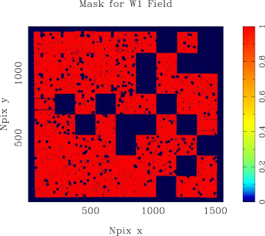
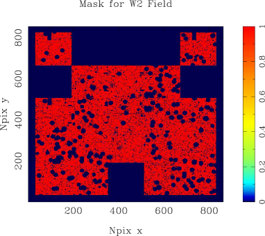
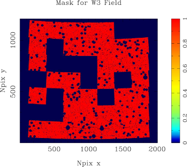
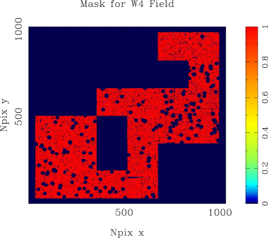
Figure 12: The pixel masks of the CFHTLenS. The top left, top right, bottom left and bottom right show the masks for the W1, W2, W3 and W4 fields, respectively. The red area shows the observed footprint.

Appendix C Maps for the W2-W4 CFHTLenS fields

In the following we show aperture maps for the remaining CFHTLenS fields. The row are identically structured as in Figs 3 and 4, but we only show the signal-to-noise map in the left column and the inverse variance weight map in the right column.

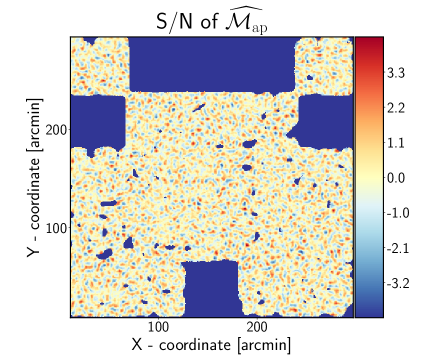
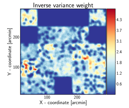
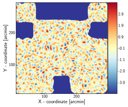
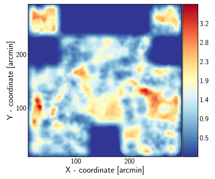
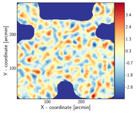
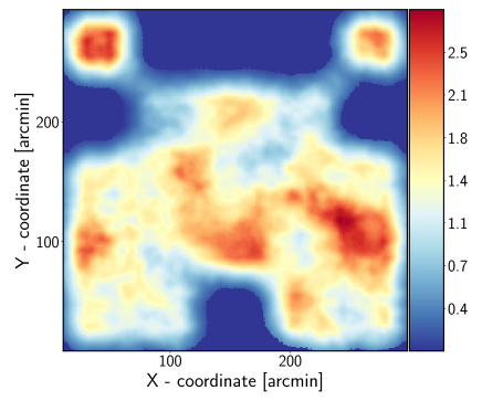
Figure 13: Signal-to-noise and aperture weight map of the W2 field of the CFHTLenS data.

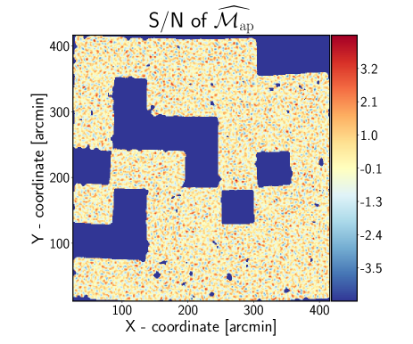
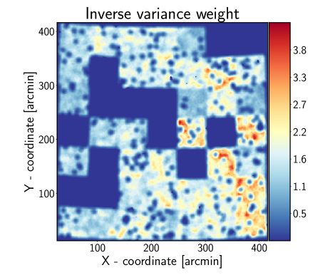
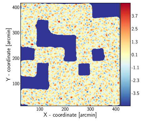
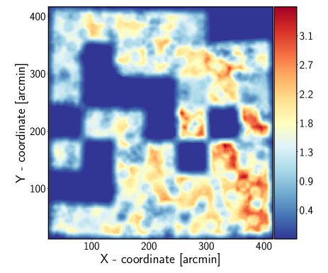
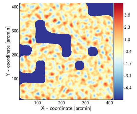
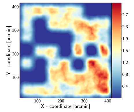
Figure 14: Signal-to-noise and aperture weight map of the W3 field of the CFHTLenS data.

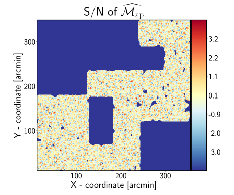
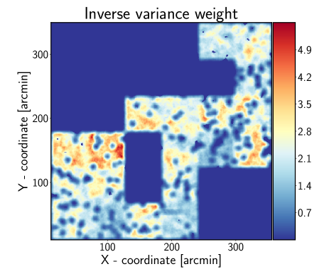
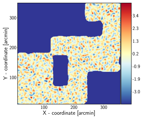
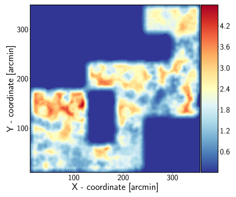
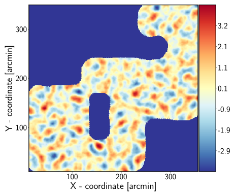
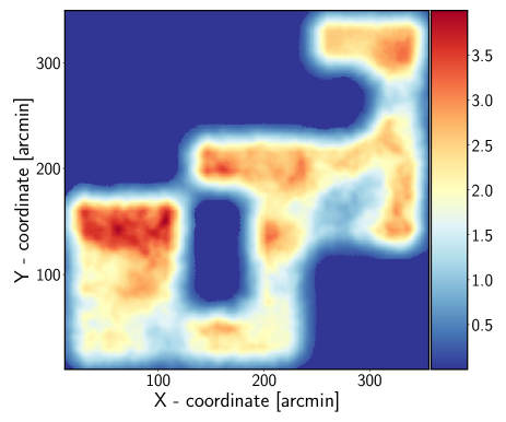
Figure 15: Signal-to-noise and aperture weight map of the W4 field of the CFHTLenS data.

References

- Aihara et al. (2018) Aihara H. et al., 2018, Publications of the ASJ, 70, S4
- Bacon, Refregier & Ellis (2000) Bacon D. J., Refregier A. R., Ellis R. S., 2000, MNRAS, 318, 625
- Bartelmann & Schneider (2001) Bartelmann M., Schneider P., 2001, Phys. Rep. , 340, 291
- Blandford et al. (1991) Blandford R. D., Saust A. B., Brainerd T. G., Villumsen J. V., 1991, MNRAS, 251, 600
- Byun et al. (2017) Byun J., Eggemeier A., Regan D., Seery D., Smith R. E., 2017, MNRAS, 471, 1581
- Crittenden et al. (2001) Crittenden R. G., Natarajan P., Pen U.-L., Theuns T., 2001, ApJ, 559, 552
- Crocce, Pueblas & Scoccimarro (2006) Crocce M., Pueblas S., Scoccimarro R., 2006, MNRAS, 373, 369
- Dodelson (2003) Dodelson S., 2003, Modern cosmology. Academic Press
- Dodelson (2017) Dodelson S., 2017, Gravitational Lensing. Cambridge University Press
- Friedrich et al. (2016) Friedrich O., Seitz S., Eifler T. F., Gruen D., 2016, MNRAS, 456, 2662
- Fu et al. (2014) Fu L. et al., 2014, MNRAS, 441, 2725
- Hartlap, Simon & Schneider (2007) Hartlap J., Simon P., Schneider P., 2007, A&A, 464, 399
- Hetterscheidt, M. et al. (2005) Hetterscheidt, M., Erben, T., Schneider, P., Maoli, R., Van Waerbeke, L., Mellier, Y., 2005, A&A, 442, 43
- Heymans et al. (2012) Heymans C. et al., 2012, MNRAS, 427, 146
- Hikage et al. (2019) Hikage C. et al., 2019, Publications of the ASJ, 71, 43
- Hilbert et al. (2020) Hilbert S. et al., 2020, Monthly Notices of the Royal Astronomical Society, 493, 305
- Hilbert et al. (2009) Hilbert S., Hartlap J., White S. D. M., Schneider P., 2009, A&A, 499, 31
- Hilbert et al. (2012) Hilbert S., Marian L., Smith R. E., Desjacques V., 2012, MNRAS, 426, 2870
- Hilbert, Metcalf & White (2007) Hilbert S., Metcalf R. B., White S. D. M., 2007, MNRAS, 382, 1494
- Hildebrandt et al. (2017) Hildebrandt H. et al., 2017, MNRAS, 465, 1454
- Jain & Seljak (1997) Jain B., Seljak U., 1997, ApJ, 484, 560
- Jarvis, Bernstein & Jain (2004) Jarvis M., Bernstein G., Jain B., 2004, MNRAS, 352, 338
- Kacprzak et al. (2016) Kacprzak T. et al., 2016, MNRAS, 463, 3653
- Kaiser (1995) Kaiser N., 1995, ApJL, 439, L1
- Kaiser (1998) Kaiser N., 1998, ApJ, 498, 26
- Kaiser, Wilson & Luppino (2000) Kaiser N., Wilson G., Luppino G. A., 2000, arXiv e-prints, astro
- Kayo, Takada & Jain (2013) Kayo I., Takada M., Jain B., 2013, MNRAS, 429, 344
- Kilbinger, Bonnett & Coupon (2014) Kilbinger M., Bonnett C., Coupon J., 2014, ascl:1402.026
- Kilbinger et al. (2013) Kilbinger M. et al., 2013, MNRAS, 430, 2200
- Kilbinger & Schneider (2005) Kilbinger M., Schneider P., 2005, A&A, 442, 69
- Kilbinger, Schneider & Eifler (2006) Kilbinger M., Schneider P., Eifler T., 2006, A&A, 457, 15
- Komatsu et al. (2009) Komatsu E. et al., 2009, ApJS, 180, 330
- Laureijs et al. (2011) Laureijs R. et al., 2011, arXiv e-prints, arXiv:1110.3193
- LSST (2009) LSST, 2009, ArXiv e-prints, arXiv:0912.0201
- Marian et al. (2013) Marian L., Smith R. E., Hilbert S., Schneider P., 2013, MNRAS, 432, 1338
- Massey et al. (2013) Massey R. et al., 2013, MNRAS, 429, 661
- Miller et al. (2013) Miller L. et al., 2013, MNRAS, 429, 2858
- Sato et al. (2011) Sato M., Takada M., Hamana T., Matsubara T., 2011, ApJ, 734, 76
- Schneider (1996) Schneider P., 1996, MNRAS, 283, 837
- Schneider (2006) Schneider P., 2006, in Saas-Fee Advanced Course 33: Gravitational Lensing: Strong, Weak and Micro, Meylan G., Jetzer P., North P., Schneider P., Kochanek C. S., Wambsganss J., eds., pp. 269–451
- Schneider & Kilbinger (2007) Schneider P., Kilbinger M., 2007, A&A, 462, 841
- Schneider & Lombardi (2003) Schneider P., Lombardi M., 2003, A&A, 397, 809
- Schneider et al. (1998) Schneider P., van Waerbeke L., Jain B., Kruse G., 1998, MNRAS, 296, 873
- Schneider et al. (2002) Schneider P., van Waerbeke L., Kilbinger M., Mellier Y., 2002, A&A, 396, 1
- Schneider, van Waerbeke & Mellier (2002) Schneider P., van Waerbeke L., Mellier Y., 2002, A&A, 389, 729
- Schneider, P., Eifler, T. & Krause, E. (2010) Schneider, P., Eifler, T., Krause, E., 2010, A&A, 520, A116
- Scoccimarro (1998) Scoccimarro R., 1998, MNRAS, 299, 1097
- Sefusatti et al. (2006) Sefusatti E., Crocce M., Pueblas S., Scoccimarro R., 2006, PRD, 74, 023522
- Seitz, Schneider & Ehlers (1994) Seitz S., Schneider P., Ehlers J., 1994, Classical and Quantum Gravity, 11, 2345
- Seljak & Zaldarriaga (1996) Seljak U., Zaldarriaga M., 1996, ApJ, 469, 437
- Semboloni et al. (2011) Semboloni E., Hoekstra H., Schaye J., van Daalen M. P., McCarthy I. G., 2011, MNRAS, 417, 2020
- Smith (2009) Smith R. E., 2009, MNRAS, 1337
- Smith & Marian (2015) Smith R. E., Marian L., 2015, MNRAS, 454, 1266
- Smith et al. (2014) Smith R. E., Reed D. S., Potter D., Marian L., Crocce M., Moore B., 2014, MNRAS, 440, 249
- Springel (2005) Springel V., 2005, MNRAS, 364, 1105
- Takada & Jain (2003) Takada M., Jain B., 2003, ApJL, 583, L49
- Takahashi et al. (2011) Takahashi R. et al., 2011, ApJ, 726, 7
- Taylor, Joachimi & Kitching (2013) Taylor A., Joachimi B., Kitching T., 2013, MNRAS, 432, 1928
- Taylor & Watts (2001) Taylor A. N., Watts P. I. R., 2001, MNRAS, 328, 1027
- Tegmark, Taylor & Heavens (1997) Tegmark M., Taylor A. N., Heavens A. F., 1997, ApJ, 480, 22
- Troxel & Ishak (2015) Troxel M. A., Ishak M., 2015, Phys. Rep. , 558, 1
- Troxel et al. (2018) Troxel M. A. et al., 2018, PRD, 98, 043528
- Van Waerbeke et al. (2000) Van Waerbeke L. et al., 2000, A&A, 358, 30
- Wittman et al. (2000) Wittman D. M., Tyson J. A., Kirkman D., Dell’Antonio I., Bernstein G., 2000, Nature, 405, 143
- Zhang et al. (2007) Zhang P., Liguori M., Bean R., Dodelson S., 2007, PRL, 99, 141302