Challenges in Semileptonic $\bm{B}$ Decays  MITP/20-035

Abstract

Two of the elements of the Cabibbo-Kobayashi-Maskawa quark mixing matrix, $|V_{ub}|$ and $|V_{cb}|$, are extracted from semileptonic $B$ decays. The results of the $B$ factories, analysed in the light of the most recent theoretical calculations, remain puzzling, because for both $|V_{ub}|$ and $|V_{cb}|$ the exclusive and inclusive determinations are in clear tension. Further, measurements in the $\tau$ channels at Belle, Babar, and LHCb show discrepancies with the Standard Model predictions, pointing to a possible violation of lepton flavor universality. LHCb and Belle II have the potential to resolve these issues in the next few years. This article summarizes the discussions and results obtained at the MITP workshop held on April 9–13, 2018, in Mainz, Germany, with the goal to develop a medium-term strategy of analyses and calculations aimed at solving the puzzles. Lattice and continuum theorists working together with experimentalists have discussed how to reshape the semileptonic analyses in view of the much higher luminosity expected at Belle II, searching for ways to systematically validate the theoretical predictions in both exclusive and inclusive $B$ decays, and to exploit the rich possibilities at LHCb.

1 Executive Summary

The magnitudes of two of the elements of the Cabibbo-Kobayashi-Maskawa (CKM) quark mixing matrix Cabibbo:1963yz ; Kobayashi:1973fv , $|V_{ub}|$ and $|V_{cb}|$, are extracted from semileptonic $B$-meson decays. The results of the $B$ factories, analysed in the light of the most recent theoretical calculations, remain puzzling, because – for both $|V_{ub}|$ and $|V_{cb}|$ – the determinations from exclusive and inclusive decays are in tension by about 3$\sigma$. Recent experimental and theoretical results reduce the tension, but the situation remains unclear. Meanwhile, measurements in the semitauonic channels at Belle, Babar, and LHCb show discrepancies with the Standard Model (SM) predictions, pointing to a possible violation of lepton-flavor universality. LHCb and the upcoming experiment Belle II have the potential to resolve these issues in the next few years.

Thirty-five participants met at the Mainz Institute for Theoretical Physics to develop a medium-term strategy of analyses and calculations aimed at the resolution of these issues. Lattice and continuum theorists discussed with experimentalists how to reshape the semileptonic analyses in view of the much larger luminosity expected at Belle II and how to best exploit the new possibilities at LHCb, searching for ways to systematically validate the theoretical predictions, to confirm new physics indications in semitauonic decays, and to identify the kind of new physics responsible for the deviations.

Format of the workshop

The program took place during a period of five days, allowing for ample discussion time among the participants. Each of the five workshop days was devoted to specific topics: the inclusive and exclusive determinations of $|V_{cb}|$ and $|V_{ub}|$, semitauonic $B$ decays and how they can be affected by new physics, as well as related subjects such as purely leptonic $B$ decays and heavy quark masses. In the mornings, we had overview talks from the experimental and theoretical sides, reviewing the main aspects and summarizing the state of the art. In the late afternoon, we organized discussion sessions led by experts of the various topics, addressing questions that have been brought up before or during the morning talks.

Exclusive heavy-to-heavy decays

The $B\to D^{(*)}\ell\nu$ decays have received significant attention in the last few years. New Belle results for the $q^{2}$ and angular distributions have allowed studies of the role played by the parametrization of the form factors in the extraction of $|V_{cb}|$. It turns out that the extrapolation to zero-recoil is very sensitive to the parametrization employed, a problem that can be solved only by precise calculations of the form factors at non-zero recoil. Until these are completed, the situation remains unclear, with repercussions on the calculation of $R(D^{*})$ as well, with diverging views on the theoretical uncertainty of present estimates based on Heavy Quark Effective Theory (HQET) expressions.

Beside a critical reexamination of these recent developments, we discussed several incremental and qualitative improvements in lattice QCD, also in baryonic decays. Though unlikely to carry much weight in determining $|V_{cb}|$, the latter offer great opportunities to test lepton-flavor universality violation (LFUV) and lattice QCD. The discussions also addressed the fact that QCD errors are now almost as small as effects from QED. Thus, further improvement must be theoretically made by properly studying the effect of QED radiation, especially the treatment of soft photons and photons that are neither soft nor hard and their sensitivity to the meson wave functions.

Concerning studies of LFUV, we discussed the role played by higher excited charmed states in establishing new physics and the challenges that the present $R(D^{(*)})$ measurements represent for model building.

Exclusive heavy-to-light decays

This determination of $|V_{ub}|$ relies on nonperturbative calculations of the form factor of $B\to\pi\ell\nu$, which is the most precise channel. We discussed the status of the light-cone sum rule (LCSR) calculations and several recent improvements in lattice QCD, in particular the most recent results from the Fermilab Lattice & MILC Collaborations and from the RBC & UKQCD Collaborations, as well as future prospects. The Fermilab/MILC calculation alone leads to a remarkably small total error on $|V_{ub}|$, about $4\%$. While at present the most precise extraction of $|V_{ub}|$ comes from $B\to\pi\ell\nu_{\ell}$, it is worth considering the channel $B_{s}\to K\ell\nu$ as well, because here the lattice-QCD calculations are affected by somewhat smaller uncertainties. $B_{s}\to K\ell\nu$ can be accessible at Belle II in a run at the $\Upsilon(5S)$ and a precision of about 5–10% could be achieved with $1~{}\text{fb}^{-1}$. On the other hand, LHCb has an ongoing analysis of the ratio $B(B_{s}\to K\ell\nu)/B(B_{s}\to D_{s}\ell\nu)$, which will provide a new determination of $|V_{ub}/V_{cb}|$. This approach follows the success that LHCb demonstrated for semileptonic baryon decays via the precise measurement of the ratio $B(\Lambda_{b}\to p\mu\nu)/(\Lambda_{b}\to\Lambda_{c}\mu\nu)$ in the high-$q^{2}$ region. This measurement, combined with precise lattice-QCD calculations of the form factors, allowed the extraction of ratio $|V_{ub}/V_{cb}|$ with an uncertainty of $7\%$. We discussed also other channels, in particular how to study $B\to\pi\pi\ell\nu$ including the resonant structures. Careful studies of other heavy-to-light channels will also be crucial to improve the signal model for the inclusive $|V_{ub}|$ measurements.

Inclusive heavy-to-heavy decays

The theoretical predictions in this case are based on an operator product expansion. Theoretical uncertainties already dominate current determinations, and better control of all higher-order corrections is needed to reduce them. In this respect, it would be important to have the perturbative-QCD corrections to the complete coefficient of the Darwin operator and to check the treatment of QED radiation in the experimental analyses. A full $O(\alpha_{s}^{3})$ calculation of the total width may be within reach with recently developed techniques. From the experimental point of view, new and more accurate measurements will be most welcome, in particular to better understand the correlations between different moments and moments with different cuts. A better determination of the higher hadronic mass moments and a first measurement of the forward-backward asymmetry would benefit the global fit, as would a better understanding of higher power corrections. The importance of having global fits to the moments in different schemes and by different groups has also been stressed. This calls for an update of the $1S$ scheme fit and could lead to a cross-check of the present theoretical uncertainties. Lattice QCD already provides inputs to the fit with the calculation of the heavy quark masses, which have been reviewed. New developments discussed at the workshop may soon be able to provide additional information that can be fed into the fits, such as constraints on the heavy-quark quantities $\mu_{\pi}^{2}$ and $\mu_{G}^{2}$. The two main approaches are i) computing inclusive rates directly with lattice QCD and ii) using the heavy quark expansion for meson masses, precisely computed at different quark mass values. The state of theoretical calculations for inclusive semitauonic decays has also been discussed, as they represent an important cross-check of the LFUV signals.

Inclusive heavy-to-light decays

This determination is based on various well-founded theoretical methods, most of which agree well. The 2017 endpoint analysis by BaBar seems to challenge this consolidated picture, suggesting discrepancies between some of the methods and a lower value of $|V_{ub}|$. For the future, the complete NNLO corrections in the full phase space should be implemented and the various methods should be upgraded in order to make the best use of the Belle II differential data based on much higher statistics. These data will make it possible to test the various methods and to calibrate them, as they will contain information on the shape functions. The SIMBA and NNVub methods seem to have the potential to fully exploit the $B\to X_{u}\ell\nu$ (and possibly radiative) measurements through combined fits to the shape function(s) and $|V_{ub}|$. The separation of $B^{\pm}$ and $B^{0}$ in the experimental analyses will certainly help to constrain weak annihilation, but the real added value of Belle II could be precise measurements of kinematic distributions in $M_{X}$, $q^{2}$, $E_{l}$, etc. A detailed measurement of the high $q^{2}$ tail might be very useful, also in view of attempts to check quark-hadron duality. Experimentally, better hybrid (inclusive+exclusive) Monte Carlos are badly needed; $s$-$\bar{s}$ popping should be investigated to develop a better understanding of kaon vetos. The $b\to c$ background will be measured better, which will benefit these analyses.

Leptonic decays

The measurement of $B\to\tau\nu$ is not yet competitive with semileptonic decays for measuring $|V_{ub}|$, because of a 20% error on the rate. Belle II will improve on this. The corresponding lattice-QCD calculation is however very precise, with an error below 1%, according to the 2019 report from FLAG Aoki:2019cca and based mainly on a result from Fermilab/MILC that was presented at the workshop. That said, the mode is useful today to model builders trying to understand new physics explanations of the tension between inclusive and exclusive determinations of $|V_{ub}|$. Belle II will also access $B\to\mu\nu(\gamma)$ with the possibility to reach an uncertainty on the branching fraction of about $5\%$ with $50~{}ab^{-1}$, allowing for a new determination of $|V_{ub}|$ in the long term. We discussed also the LHCb contribution to leptonic decays with the process $B\to\mu\mu\mu\nu_{\mu}$ where two of the muons come from virtual $\gamma$ or light vector meson decays. A study of this channel has been published in  Aaij:2018pKa and a very stringent upper limit obtained, inconsistent with the existing branching fraction predictions, calls for new reliable theoretical calculations.

2 Heavy-to-heavy exclusive decays

The aim of this section is to present an overview of $b\to c$ exclusive decays. After an introduction to the parametrization of the relevant form factors between hadronic states we describe the status of current lattice QCD calculations with particular focus on $B\to D^{*}$ and $\Lambda_{b}\to\Lambda_{c}$. Next, we discuss experimental measurements of $B\to D^{(*)}$ semileptonic decays with special focus on the ratios $R(D^{(*)})$, and several phenomenological aspects of these decays: the extraction of $V_{cb}$, theoretical predictions for $R(D^{(*)})$, the role of $B\to D^{**}$ transitions and constraints on new physics. We also briefly discuss the information that is required to reproduce results presented in experimental analyses and to incorporate older measurements into approaches based on modern form factor parametrizations. We conclude with the description of HAMMER, a tool designed to more easily calculate the change in signal acceptancies, efficiencies and signal yields in the presence of new physics.

2.1 Parametrization of the form factors

In this section, we introduce the form factors for the hadronic matrix elements that arise in semileptonic decays. Several different notations appear in the literature, often using different conventions depending on whether the final-state meson is heavy (e.g., $D$) or light (e.g., $\pi$). A general decomposition relies, however, only on Lorentz covariance and other symmetry properties of the matrix elements. As discussed below, it is advantageous to choose the Lorentz structure so that the form factors have definite parity and spin.

In this spirit, let us consider the matrix elements for a meson decay $B_{(l)}\to X^{(\ast)}\ell\nu$, where the quark content of the $\bar{B}$ is $bl$ with $l$ a light quark ($u$, $d$, or $s$), and the quark content of the $X$ is $\bar{q}l$ where $q$ can be either a light quark or the $c$ quark. The desired decomposition can be written as

$$\left\langle X(p^{\prime})|S|B_{(l)}(p)\right\rangle =\frac{M^{2}-m^{2}}{m_{b}-m_{q}}f_{0}(q^{2}),$$ (1)

$$\left\langle X(p^{\prime})|V^{\mu}|B_{(l)}(p)\right\rangle =\left[(p+p^{\prime})^{\mu}-\frac{M^{2}-m^{2}}{q^{2}}q^{\mu}\right]f_{+}(q^{2})+\frac{M^{2}-m^{2}}{q^{2}}q^{\mu}\,f_{0}(q^{2}),$$ (2)

$$\left\langle X(p^{\prime})|T^{\mu\nu}|B_{(l)}(p)\right\rangle =2\frac{p^{\mu}p^{\prime\nu}-p^{\nu}p^{\prime\mu}}{M+m}f_{T}(q^{2}),$$ (3)

$$\left\langle X^{\ast}(p^{\prime})|P|B_{(l)}(p)\right\rangle =\frac{2m}{m_{b}+m_{q}}(\epsilon^{\ast}\cdot q)A_{0}(q^{2}),$$ (4)

$$\left\langle X^{\ast}(p^{\prime})|V^{\mu}|B_{(l)}(p)\right\rangle =\frac{2i}{M+m}\varepsilon^{\mu\nu\alpha\beta}\epsilon^{\ast}_{\nu}p_{\alpha}p^{\prime}_{\beta}\,V(q^{2}),$$ (5)

$$\left\langle X^{\ast}(p^{\prime})|A^{\mu}|B_{(l)}(p)\right\rangle =2m\frac{\epsilon^{\ast}\cdot q}{q^{2}}q^{\mu}\,A_{0}(q^{2})+(M+m)\left(\epsilon^{\ast\mu}-\frac{\epsilon^{\ast}\cdot q}{q^{2}}q^{\mu}\right)A_{1}(q^{2})$$

$$-\frac{\epsilon^{\ast}\cdot q}{M+m}\left[(p+p^{\prime})^{\mu}-\frac{M^{2}-m^{2}}{q^{2}}q^{\mu}\right]A_{2}(q^{2}),$$ (6)

$$\left\langle X^{\ast}(p^{\prime})|T^{\mu\nu}|B_{(l)}(p)\right\rangle =i\epsilon^{\mu\nu\sigma\rho}\left\{\epsilon^{\ast}_{\sigma}\left[(p+p^{\prime})_{\rho}T_{1}(q^{2})-\vphantom{\frac{M^{2}-m^{2}}{q^{2}}}\right.\right.$$

$$\left.\left.\hskip 20.00003ptq_{\rho}\frac{M^{2}-m^{2}}{q^{2}}\left(T_{1}(q^{2})-T_{2}(q^{2})\right)\right]\right.$$ (7)

$$+ \left.(\epsilon^{\ast}\cdot p)\frac{(p+p^{\prime})_{\sigma}q_{\rho}}{q^{2}}\left[T_{1}(q^{2})-T_{2}(q^{2})-\frac{q^{2}}{M^{2}-m^{2}}T_{3}(q^{2})\right]\right\},$$

where $q^{\mu}=(p-p^{\prime})^{\mu}$ is the momentum transfer, $S=\bar{b}q$ is the scalar current, $P=\bar{b}\gamma^{5}q$ is the pseudoscalar current, $V^{\mu}=\bar{b}\gamma^{\mu}q$ is the vector current, $A^{\mu}=\bar{b}\gamma^{\mu}\gamma_{5}c$ is the axial current, $T^{\mu\nu}=\bar{b}\sigma^{\mu\nu}c$ is the tensor current, $m_{q}$ is the mass of the quark $q$, $M$ is the mass of the parent meson ($B$ in this case), $m$ (without subscript) is the mass of the daughter meson, and $r=m/M$. Contracting Eqs. (2) and (6) with $q_{\mu}$ and using the appropriate Ward identities shows that the scalar form factor, $f_{0}$, and pseudoscalar form factor, $A_{0}$, appear in the vector and axial vector transitions. The $J^{P}$ quantum numbers of the form factors are given in Table 1.

Table 1: Quantum numbers of various meson form factors.

	$0^{+}$	$0^{-}$	$1^{-}$	$1^{+}$	$2^{+}$
$B_{(l)}\to X\ell\bar{\nu}$	$f_{0}$	–	$f_{+}$	–	$f_{T}$
$B_{(l)}\to X^{\ast}\ell\bar{\nu}$	–	$A_{0}$	$V_{0}$	$A_{1},A_{2}$	$T_{1},T_{2},T_{3}$

The tensor form factors in Eqs. (3) and (7) appear in extensions of the Standard Model.

One can impose bounds on the shape of these form factors by using QCD dispersion relations for a generic decay $H_{b}\to H_{q}\ell\bar{\nu}$. Since the amplitude for production of $H_{b}H_{q}$ from a virtual $W$ boson is determined by the analytic continuation of the form factors from the semileptonic region of momentum transfer $m_{\ell}^{2}<q^{2}<M^{2}-m^{2}$ to the pair production region $q^{2}\geq M^{2}+m^{2}$, one can find constraints in the pair-production region, amenable to perturbative QCD calculations, and then propagate the constraint to the semileptonic region by using analyticity. The result of this process applied to the form factors is the model-independent Boyd-Grinstein-Lebed (BGL) parametrization Boyd:1995cf ; Boyd:1997kz , which expands a form factor $F(z)$ in the dimensionless variable $z$ as

$$F(z) =\frac{1}{B_{F}(z)\phi_{F}(z)}\sum_{j=0}^{\infty}a^{F}_{j}z^{j},$$ (8)

$$z(q^{2};t_{0}) =\frac{\sqrt{t_{+}-q^{2}}-\sqrt{t_{-}-q^{2}}}{\sqrt{t_{+}-q^{2}}+\sqrt{t_{+}-t_{0}}},$$ (9)

where $t_{\pm}=(M\pm m)^{2}$, $B_{F}(z)$ are known as the Blaschke factors, which incorporate the below- or near-threshold Caprini:2017ins poles in the $s$-channel process $\ell\nu\to\bar{B}X$, and $\phi_{F}(z)$ is called the outer function. The poles, and hence the Blaschke factor, depend on the spin and the parity of the intermediate state, which is why it is useful to use fixed $J^{P}$ for the form factors. See Sec. 3.5.5 for more details. Of course, in practical applications the series (8) is truncated at some power $z^{n_{F}}$.

By taking certain linear combinations of form factors with the same spin and parity one obtains the BGL notation for the helicity amplitudes,

$$f^{\text{BGL}}_{+} =f_{+},$$ (10)

$$f^{\text{BGL}}_{0} =(M^{2}-m^{2})f_{0},$$ (11)

$$g =\frac{2}{M+m}V,$$ (12)

$$f =(M+m)A_{1},$$ (13)

$$\mathcal{F}_{1} =M(M+m)(w-r)A_{1}-\frac{2Mm(w^{2}-1)}{1+r}A_{2},$$ (14)

$$\mathcal{F}_{2} =2A_{0},$$ (15)

leaving aside the (BSM) tensor form factors. Here the velocity transfer

$$w=v_{M}\cdot v_{m}=\frac{M^{2}+m^{2}-q^{2}}{2Mm},$$ (16)

with $v_{M}=p/M$ and $v_{m}=p^{\prime}/m$, is often used in heavy-to-heavy decays. For heavy-to-light decays it can be helpful to work with the energy of the daughter meson in the rest frame of the parent, i.e.,

$$E=p^{\prime}\cdot v_{M}=\frac{M^{2}+m^{2}-q^{2}}{2M}.$$ (17)

These form factors are subject to three kinematic constraints, namely

$$(M^{2}-m^{2})f^{\text{BGL}}_{+}(q^{2}=0) =f^{\text{BGL}}_{0}(q^{2}=0),$$ (18)

$$(M-m)f(q^{2}=q_{\text{max}}^{2}) =\mathcal{F}_{1}(q^{2}=q_{\text{max}}^{2}),$$ (19)

$$\frac{2}{M^{2}-m^{2}}\mathcal{F}_{1}(q^{2}=0) =\mathcal{F}_{2}(q^{2}=0),$$ (20)

where $q^{2}_{\text{max}}=(M-m)^{2}$, corresponding to $w=1$ and $E=m$.

The variable $z$ can also be expressed via $w$,

$$z=\frac{\sqrt{w+1}-\sqrt{2N}}{\sqrt{w+1}+\sqrt{2N}},$$ (21)

where $N=(t_{+}-t_{0})/(t_{+}-t_{-})$, is real for $q^{2}\leq(M+m)^{2}$, and it becomes a pure phase beyond that limit. The constant $t_{0}$ defines the point at which $z=0$. Often $t_{0}=t_{-}$, one end of the kinematic range, so $z$ ranges from 0 at maximum $q^{2}$ to $z_{\text{max}}=(1-\sqrt{r})^{2}/(1+\sqrt{r})^{2}$ when $m_{\ell}\approx 0$. Alternatively, the choice $t_{0}=(M+m)(\sqrt{M}-\sqrt{m})^{2}$ sets $z=0$ exactly in the middle of the kinematic range. Even for $B\to\pi\ell\nu$, $z$ is always a small quantity, which ensures a fast convergence of the power series defined in (8).

Unitarity constraints from the QCD dispersion relations are translated into constraints for the coefficients of the BGL expansion. In general,

$$\sum^{\infty}_{j=0}\left(a^{F}_{j}\right)^{2}\leq 1,$$ (22)

for each form factor $F$, but in the particular case of $\bar{B}\to D^{\ast}\ell\bar{\nu}$ the bound becomes

$$\sum^{\infty}_{j=0}\left[\left(a^{f}_{j}\right)^{2}+\left(a^{\mathcal{F}_{1}}_{j}\right)^{2}\right]\leq 1,$$ (23)

for the $f$ and $\mathcal{F}_{1}$ form factors, because they have the same quantum numbers. These bounds are known as the weak unitarity constraints.

A modification of the BGL parametrization by Bourrely, Lellouch and Caprini (BCL) Bourrely:2008za is often chosen in analyses of heavy-to-light decays. The BCL parametrization improves BGL by fixing two artifacts of the truncated BGL series. In particular, it removes an unphysical singularity at the pair production threshold and corrects the large $q^{2}$ behavior (see Lepage:1980fj ; Akhoury:1993uw ) in the functional form. These two modifications improve the convergence of the expansion. However, the kinematic range is much more constrained in the heavy-to-heavy case, and lies farther from both the production threshold and the large $q^{2}$ region. Therefore, the presence of far singularities or an incorrect asymptotic behavior are not expected to spoil the $z$-expansion in that case.

In the heavy-to-heavy case, one can sharpen the weak unitarity constraints on the BGL coefficients using heavy quark symmetry (HQS) which relates the different $B^{(*)}\to D^{(*)}\ell\bar{\nu}$ channels and their form factors: each form factor is either proportional to the Isgur-Wise function $\xi(w)$ or zero. Using heavy quark effective theory (HQET) one can improve the precision by introducing radiative and power (i.e. in inverse powers of the heavy masses) corrections. Then we can define any form factor in such a way that it admits the expansion in both $\alpha_{s}$ and the heavy quark masses

$$F(w)=\xi(w)\left(1+c_{\alpha_{s}}\frac{\alpha_{s}}{\pi}+c_{b}\frac{\Lambda_{\textrm{QCD}}}{m_{b}}+c_{c}\frac{\Lambda_{\textrm{QCD}}}{m_{c}}+\cdots\right).$$ (24)

These expansions can be used to link the $z$ expansion coefficients of different form factors, leading to the so-called strong unitarity constraints Caprini:1997mu ; Bigi:2017jbd . The power corrections depend on subleading Isgur-Wise functions that have been estimated with QCD sum rules Neubert:1992wq ; Neubert:1992pn ; Ligeti:1993hw .

Previous analyses of $B\to D^{\ast}\ell\nu$ have used the Caprini-Lellouch-Neubert (CLN) parametrization Caprini:1997mu . CLN employ a notation for the form factors that satisfies (24),

$$S^{\text{CLN}}_{1} =\frac{f^{\text{BGL}}_{0}}{M^{2}(1-r)\sqrt{r}(1+w)}, P^{\text{CLN}}_{1}=\frac{\sqrt{r}}{1+r}\mathcal{F}_{2},$$ (25)

$$V^{\text{CLN}}_{1} =\frac{2\sqrt{r}}{1+r}f^{\text{BGL}}_{+}, V^{\text{CLN}}_{4}=M\sqrt{r}g,$$ (26)

$$A^{\text{CLN}}_{1} =\frac{f}{M\sqrt{r}(1+w)}, A^{\text{CLN}}_{5}=\frac{\mathcal{F}_{1}}{M^{2}(1-r)\sqrt{r}(1+w)},$$ (27)

$$R^{\text{CLN}}_{1} =\frac{V^{\text{CLN}}_{4}}{A^{\text{CLN}}_{1}}, R^{\text{CLN}}_{2}=\frac{w-r}{w-1}-\frac{(1-r)}{w-1}\frac{A^{\text{CLN}}_{5}}{A^{\text{CLN}}_{1}},$$ (28)

where the letter naming the form factor ($S$, $P$, $V$ and $A$) encodes its quantum numbers (scalar, pseudoscalar, vector and axial vector), and $R^{\text{CLN}}_{1,2}$ are two convenient ratios of form factors. Sometimes the ratio $R^{\text{CLN}}_{0}=P^{\text{CLN}}_{1}/A^{\text{CLN}}_{1}$ is considered.

In the CLN parametrization the strong unitarity constraints obtained with HQET at NLO are used to remove some of the coefficients of the $z$ expansion. Further, specific numerical coefficients are introduced in a polynomial in $w$ for $R_{1,2}^{\text{CLN}}$. The numerical values were determined using information available in 1997, which has been partly superseded but not updated. The numerical values also omit error estimates (which were discussed in the original CLN paper Caprini:1997mu , although in an optimistic manner) because at the time the experimental statistical errors dominated, which is no longer the case. A consensus of the workshop recommends that CLN no longer be used, certainly not unless the numerical coefficients have been updated and the ensuing theoretical uncertainties are accounted for. It is better to use a general form of the $z$ expansion.

HQET naturally presents another basis for the form factors of the $\bar{B}\to D^{(\ast)}\ell\bar{\nu}$ processes. Using velocities instead of momenta and otherwise mimicking the Lorentz structure of Eqs.(2), (5), and (6), the notation is $h_{+}$ and $h_{-}$ for $\bar{B}\to D\ell\bar{\nu}$, and $h_{V}$ and $h_{A_{1,2,3}}$ for $\bar{B}\to D^{\ast}\ell\bar{\nu}$. In the heavy quark limit, these form factors tend to

$$h_{X}(w)=\eta(\alpha_{s})\xi(w)+O\big{(}\frac{\Lambda_{\rm QCD}}{m_{b,c}}\big{)},$$ (29)

for $X=+$, $A_{1}$, $A_{3}$, $V$, and

$$h_{Y}(w)=\beta(\alpha_{s})\xi(w)+O\big{(}\frac{\Lambda_{\rm QCD}}{m_{b,c}}\big{)},$$ (30)

with $Y=-$, $A_{2}$. Here $\eta(\alpha_{s})=1+O(\alpha_{s})$, while $\beta(\alpha_{s})=O(\alpha_{s})$. In this representation, the identities expressed in Eqs. (18)–(20) become evident.

Finally, for the case of a baryonic decay $\Lambda_{b}\to Y_{(q)}\ell\nu$, with $Y=p,\Lambda_{c}$, we define

$$\left\langle Y(p^{\prime})|S|\Lambda_{b}(p)\right\rangle =\bar{u}_{q}(p^{\prime})\frac{M-m}{m_{b}-m_{q}}f_{0}(q^{2})u_{b}(p),$$ (31)

$$\left\langle Y(p^{\prime})|P|\Lambda_{b}(p)\right\rangle =\bar{u}_{q}(p^{\prime})\gamma_{5}\frac{M+m}{m_{b}+m_{q}}g_{0}(q^{2})u_{b}(p),$$ (32)

$$\left\langle Y(p^{\prime})|V^{\mu}|\Lambda_{b}(p)\right\rangle =\bar{u}_{q}(p^{\prime})\left[(M-m)\frac{q^{\mu}}{q^{2}}f_{0}(q^{2})+\right.$$

$$\left.\frac{M+m}{s_{+}}\left((p+p^{\prime})^{\mu}-\frac{q^{\mu}}{q^{2}}(M^{2}-m^{2})\right)f_{+}(q^{2})+\right.$$

$$\left.\left(\gamma^{\mu}-2\frac{mp^{\mu}+Mp^{\prime\mu}}{s_{+}}\right)f_{\bot}(q^{2})\right]u_{b}(p),$$ (33)

$$\left\langle Y(p^{\prime})|A^{\mu}|\Lambda_{b}(p)\right\rangle =-\bar{u}_{q}(p^{\prime})\gamma_{5}\left[(M+m)\frac{q^{\mu}}{q^{2}}g_{0}(q^{2})+\right.$$

$$\left.\frac{M-m}{s_{-}}\left((p+p^{\prime})^{\mu}-\frac{q^{\mu}}{q^{2}}(M^{2}-m^{2})\right)g_{+}(q^{2})+\right.$$

$$\left.\left(\gamma^{\mu}+2\frac{mp^{\mu}-Mp^{\prime\mu}}{s_{-}}\right)g_{\bot}(q^{2})\right]u_{b}(p),$$ (34)

$$\left\langle Y(p^{\prime})|q_{\nu}T^{\mu\nu}|\Lambda_{b}(p)\right\rangle =-\bar{u}_{q}(p^{\prime})\left[\left((p+p^{\prime})^{\mu}-\frac{q^{\mu}}{q^{2}}(M^{2}-m^{2})\right)\frac{q^{2}}{s_{+}}h_{+}(q^{2})\right.$$

$$\left.+(M+m)\left(\gamma^{\mu}-2\frac{mp^{\mu}+Mp^{\prime\mu}}{s_{+}}\right)h_{\bot}(q^{2})\right]u_{b}(p),$$ (35)

where $M$ is the mass of the $\Lambda_{b}$, $m$ is the mass of the daughter baryon and $s_{\pm}=(M\pm m)^{2}-q^{2}$. The $z$ expansions for the baryonic form factors employed in Ref. Detmold:2015aaa use trivial outer functions and do not impose unitarity bounds on the coefficients of the expansion. As a result, the coefficients are unconstrained and reach values as high as $\sim 10$. See also Sec. 3.5.5.

2.2 Heavy-to-heavy form factors from lattice QCD

The lattice QCD calculation of the form factors for the semileptonic decay of a hadron uses two- and three-point correlation functions, which are constructed from valence quark propagators obtained by solving the Dirac equation on a set of gluon field configurations. Averaging the correlation functions over the gluon field configurations then yields the appropriate Feynman path integral. The two-point correlation functions give the amplitude for a hadron to be created at the time origin and then destroyed at a time $T$. The three-point correlation functions include the insertion of a current $J$ at time $t$ on the active quark line, changing the active quark from one flavor to another. Usually calculations are performed with the initial hadron at rest. Momentum is inserted at the current so that a range of momentum transfer, $q$, from initial to final hadron can be mapped out.

The three-point correlation functions (for multiple $q$ values) and the two-point correlation functions (with multiple momenta in the case of the final-state hadron) are fit as functions of $t$ and $T$ to determine the matrix elements of the currents between initial and final hadrons that yield the required form factors. An important point here is that the initial and final hadrons that we focus on are the ground-state particles in their respective channels. However, terms corresponding to excited states must be included in the fits in order to make sure that systematic effects from excited-state contamination are taken into account in the fit parameters that yield the ground-state to ground-state matrix element of $J$ and hence the form factors.

Statistical uncertainties in the form factors obtained obviously depend on the numbers of samples of gluon-field configurations on which correlation functions are calculated. To improve statistical accuracy further, calculations usually include multiple positions of the time origin for the correlation functions on each configuration. The numerical cost of the calculation of quark propagators falls as the quark mass increases and so heavy ($b$ and $c$) quark propagators are typically numerically inexpensive. The accompanying light quark propagators for heavy-light hadrons are much more expensive, especially if $u/d$ quarks with physically light masses are required. It is this cost that limits the statistical accuracy that can be obtained, especially since the statistical uncertainty for a heavy-light hadron correlation function (on a given number of gluon field configurations) also grows as the separation in mass between the heavy and light quarks increases.

A key issue for heavy-to-heavy ($b$ to $c$) form factor calculations is how to handle heavy quarks on the lattice. Discretization of the Dirac equation on a space-time lattice gives systematic discretization effects that depend on powers of the quark mass in lattice units. The size of these effects depends on the value of the lattice spacing and the power with which the effects appear (i.e., the level of improvement used in the lattice Lagrangian).

Since the $b$ quark is so heavy, its mass in lattice units will be larger than 1 on all but the finest lattices ($a<$ 0.05 fm) currently in use. Highly-improved discretizations of the Dirac equation are needed to control the discretization effects. A good example of such a lattice quark formalism is the highly improved staggered quark (HISQ) action developed by HPQCD Follana:2006rc for both light and heavy quarks with discretization errors appearing at $O(\alpha_{s}(am)^{2})$ and $O((am)^{4})$. An alternative approach is to make use of the fact that $b$ quarks are nonrelativistic inside their bound states. This means that a discretization of a nonrelativistic action (NRQCD) can be used, expanding the action to some specified order in the $b$ quark velocity. Discretization effects then depend on the scales associated with the internal dynamics and these scales are all much smaller than the $b$ quark mass. Relativistic effects can be included and discretization effects corrected at the cost of complicating the action with additional operators. A third possibility is to start from the Wilson quark action and improved versions of it but to tune the parameters (such as the quark mass) using a nonrelativistic dispersion relation for the meson, which is known as the Fermilab method ElKhadra:1996mp . This removes the leading source of mass-dependent discretization effects, whilst retaining a discretization that connects smoothly to the continuum limit. Again, improved versions of this approach (such as the Oktay-Kronfeld action Oktay:2008ex ) include additional operators.

The $c$ quark has a mass larger than $\Lambda_{\mathrm{QCD}}$ but within lattice QCD it can be treated successfully as a light quark because its mass in lattice units is less than 1 on lattices in current use (with $a<0.15$ fm). This means that, although discretization effects are visible in lattice QCD calculations with $c$ quarks, they are not large and can easily be extrapolated away accurately for a continuum result. For example, discretization effects are less than 10% at $a=0.15$ fm in calculations of the decay constant of the $D_{s}$ using the HISQ action Davies:2010ip . Purely nonrelativistic approaches to the $c$ quark are therefore not useful on the lattice. There can be some advantage for $b$-to-$c$ form factor calculations in using the same action for $b$ and $c$, however, as we discuss below.

Because lattice and continuum QCD regularize the theory in a different way, the lattice current $J$ needs a finite renormalization factor to match its continuum counterpart so that matrix elements of $J$, and form factors derived from them, can be used in continuum phenomenology. For NRQCD and Wilson/Fermilab quarks the current $J$ must be normalized using lattice QCD perturbation theory. Since this is technically rather challenging it has only been done through $O(\alpha_{s})$ and this leaves a sizeable (possibly several percent) systematic error from missing higher-order terms in the perturbation theory. If Wilson/Fermilab quarks are used for both $b$ and $c$ quarks, then arguments can be made about the approach to the heavy-quark limit that can reduce, but not eliminate, this uncertainty Harada:2001fj .

Relativistic treatments of the $b$ and $c$ quarks have a big advantage here, because $J$ can generally be normalized in a fully nonperturbative way within the lattice QCD calculation and without additional systematic errors. The advantages of this approach were first demonstrated by the HPQCD collaboration using the HISQ action to determine the decay constant of the $B_{s}$ McNeile:2012qf . The HISQ PCAC relation normalizes the axial-vector current in this case. Calculations for multiple quark masses on lattices with multiple values of the lattice spacing allow both the physical dependence of the decay constant on quark mass and the dependence of the discretization effects to be mapped out so that the physical result at the $b$ quark mass can be determined. This calculation has now been updated and extended to the $B$ meson by the Fermilab Lattice and MILC collaborations Bazavov:2017lyh , achieving better than 1% uncertainty. HPQCD is now carrying out a similar approach to $b$-to-$c$ form factor calculations McLean:2019sds , and the JLQCD collaboration is also working in that direction Kaneko:2019vkx with Möbius domain-wall quarks.

An equivalent approach, using ratios of hadronic quantities at different quark masses where normalization factors cancel, has been developed by the European Twisted Mass collaboration using the twisted-mass action Blossier:2009hg ; Bussone:2016iua for Wilson fermions.

2.2.1 $B\rightarrow D^{(*)}$ form factors from lattice QCD

Early lattice QCD calculations of $B\to D$ form factors were limited to the determination of $\mathcal{G}^{B\to D}(w)=4rf_{+}(q^{2})/(1+r)$ (with notation defined near (16)) at the zero-recoil point $w=1$. Results include the $N_{f}=2+1$ calculation of Fermilab/MILC Okamoto:2004xg ; Qiu:2013ofa and the $N_{f}=2$ calculation of Atoui et al. Atoui:2013zza . More recently Fermilab/MILC Lattice:2015rga and HPQCD Na:2015kha ; Monahan:2017uby have presented $N_{f}=2+1$ calculations of the $B\to D$ form factor at non-zero recoil based on partially overlapping subsets of the same MILC asqtad ($a^{2}$ tadpole improved) ensembles.

The Fermilab/MILC calculation Lattice:2015rga uses configurations with four different lattice spacings and with pion masses in the range $[260,670]$ MeV. The bottom and charm quarks are implemented in the Fermilab approach. The form factors $f_{+,0}^{B\to D}(w)$ are extracted from double ratios of three point functions up to a matching factor which is calculated at 1-loop in lattice perturbation theory. The results are presented in terms of three synthetic data points which can be subsequently fitted using any form factor parametrization. The systematic uncertainty due to the joint continuum-chiral extrapolation is about 1.2% and dominates the error budget.

The HPQCD calculations Na:2015kha ; Monahan:2017uby rely on ensembles with two different lattice spacings and two/three light-quark masses values, respectively. The treatment of heavy quarks is different from that used in the Fermilab/MILC papers: the bottom quark is described in NRQCD and the charm quark using HISQ. The form factors are extracted from appropriate three-point functions and the results are presented in terms of the parameters of a modified BCL $z$ expansion that incorporates dependence on lattice spacing and light-quark masses into the expansion coefficients.

In order to combine the Fermilab/MILC and HPQCD results Aoki:2019cca , it is necessary to generate a set of synthetic data which is (almost exactly) equivalent to the HPQCD calculation. The two sets of synthetic data can then be combined while taking into account the correlation due to the fact the Fermilab/MILC and HPQCD share MILC asqtad configurations. As mentioned above, dominant uncertainties are of systematic nature, implying that this correlation (whose estimate is rather uncertain) is a subdominant effect. A simultaneous fit of Fermilab/MILC and HPQCD synthetic data together with the available Belle and Babar data yields a determination of $|V_{cb}|$ with an overall 2.5% uncertainty (dominated by the experimental error which contributes about 2% to the total error).

Finally, both collaborations present values for both the $f_{+}$ and $f_{0}$ form factors, which allow for a lattice only calculation of the SM prediction for $R(D)$. The uncertainty on the Fermilab/MILC and HPQCD combined determination of $R(D)$, without experimental input, is about 2.5% and is negligible compared to current experimental errors.

The advantage of an approach in which currents can be nonperturbatively normalized has been demonstrated by HPQCD for $B_{s}\rightarrow D_{s}$ form factors in McLean:2019qcx . They use the HISQ action for all quarks, extending the method developed for decay constants. The range of heavy quark masses can be increased on successively finer lattices (keeping the value in lattice units below 1) until the full range from $c$ to $b$ is reached. The full $q^{2}$ range of the decay can also be covered by this method since the spatial momentum of the final state meson (which should also be less than 1 in lattice units) grows in step with the heavy meson/quark mass. Results from McLean:2019qcx improve on the uncertainties obtained in Monahan:2017uby with NRQCD $b$ quarks and this promising all-HISQ approach is now being extended to other processes. It is interesting to observe that the $B_{s}\to D_{s}$ form factors are very close to the $B\to D$ form factors over the entire kinematic range, see also Kobach:2019kfb ; Bordone:2019guc .

Calculations of $B\to D^{*}$ form factors at non-zero recoil are considerably more involved due to difficulties in describing the resonant $D^{*}\to D\pi$ decay. Up to now, lattice QCD simulations have focused on the single $B\rightarrow D^{*}$ form factor that contributes to the rate at zero recoil, $A_{1}(q^{2}_{max})$. The quantity generally quoted is $h_{A_{1}}(1)$ where

$$h_{A_{1}}(1)=\frac{M_{B}+M_{D^{*}}}{2\sqrt{M_{B}M_{D^{*}}}}A_{1}(q^{2}_{\text{max}})$$ (36)

The combination of the lattice QCD result and the experimental rate, extrapolated to zero recoil, yields a value for $V_{cb}$.

The Fermilab Lattice/MILC Collaborations have achieved the highest precision for this result so far Bailey:2014tva . They use improved Wilson quarks within the Fermilab approach for both $b$ and $c$ quarks and work on gluon field configurations that include $u/d$ (with equal mass) and $s$ quarks in the sea ($n_{f}=2+1$) using the asqtad action. By taking a ratio of three-point correlation functions they are able simultaneously able to improve their statistical accuracy and reduce part of the systematic uncertainty from the normalization of their current operator. Their result is $h_{A_{1}}(1)=0.906(4)(12)$ where the uncertainties are statistical and systematic respectively. Their systematic error is dominated by discretization effects. They take the systematic uncertainty from missing higher-order terms in the perturbative current matching Monahan:2012dq to be $0.1\alpha_{s}^{2}$.

The HPQCD collaboration have calculated $h_{A_{1}}(1)$ on gluon field configurations that include $n_{f}=2+1+1$ HISQ sea quarks using NRQCD $b$ quarks and HISQ $c$ quarks Harrison:2017fmw . Their result, $h_{A_{1}}(1)=0.895(10)(24)$ has a larger uncertainty, dominated by the systematic uncertainty of $0.5\alpha_{s}^{2}$ allowed for in the current matching. They were also able to calculate the equivalent result for $B_{s}\rightarrow D_{s}^{*}$, obtaining $h^{s}_{A_{1}}(1)=0.879(12)(26)$ and demonstrating that the dependence on light quark mass is small. The $B_{s}\rightarrow D_{s}^{*}$ provides a better lattice QCD comparison point than $B\rightarrow D^{*}$ because it has less sensitivity to light quark masses (in particular the $D^{*}D\pi$ “cusp”) and to the volume.

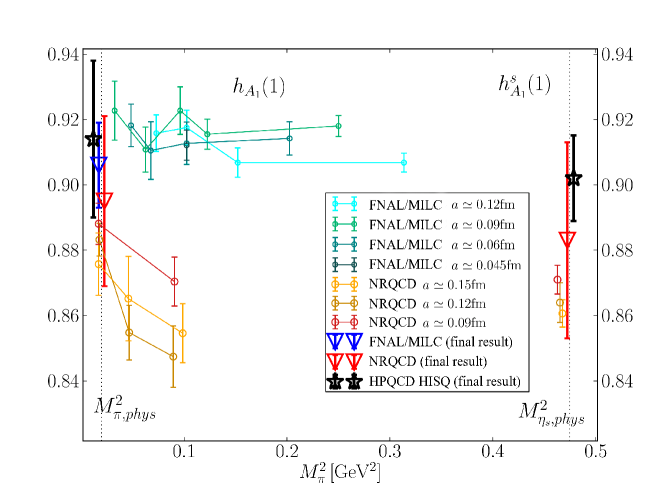
Figure 1: Plot taken from Ref. McLean:2019sds showing the comparison of lattice QCD results for $h_{A_{1}}(1)$ (left side) and $h^{s}_{A_{1}}(1)$ (right side). Raw results for $h_{A_{1}}(1)$ are from Harrison:2017fmw and Bailey:2014tva and are plotted as a function of valence (=sea) light quark mass, given by the square of $M_{\pi}$. On the right are points for $h^{s}_{A_{1}}(1)$ from Harrison:2017fmw plotted at the appropriate valence mass for the $s$ quark, but obtained at physical sea light quark masses. The final result for $h_{A_{1}}(1)$ from Bailey:2014tva , with its full error bar, is given by the inverted blue triangle. The inverted red triangles give the final results for $h_{A_{1}}(1)$ and $h^{s}_{A_{1}}(1)$ from Harrison:2017fmw . The HPQCD results of McLean:2019sds are given by the black stars.

More recently the HPQCD collaboration have used the HISQ action for all quarks, with a fully nonperturbative current normalization, to determine $h^{s}_{A_{1}}(1)$ McLean:2019sds . Their result, $h^{s}_{A_{1}}(1)=0.9020(96)(90)$ agrees well with the earlier results and has smaller systematic uncertainties. Figure 1 compares the three results.

The importance of being able to compare lattice QCD and experiment away from the zero recoil point is now clear and several lattice QCD calculations are underway, attempting to cover the full $q^{2}$ range of the decay and all 4 form factors. This includes calculations for $B\rightarrow D^{*}$ from JLQCD Kaneko:2019vkx with Möbius domain-wall quarks, Fermilab/MILC Vaquero:2019ary (see also talk at Lattice 2019) with improved Wilson/Fermilab quarks and LANL/SWME with an improved version of this formalism known as the Oktay-Kronfeld action Bhattacharya:2020xyb . Calculations for other $b\to c$ pseudoscalar-to-vector form factors, $B_{s}\rightarrow D^{*}_{s}$ McLean:2019jll and $B_{c}\rightarrow(J/\psi,\eta_{c})$ are also underway from HPQCD Lytle:2016ixw ; Colquhoun:2016osw using the all-HISQ approach. At the same time further $B\rightarrow D$ and $B_{s}\rightarrow D_{s}$ form factor calculations are in progress, including those using a variant of the Fermilab approach known as Relativistic Heavy Quarks on RBC/UKQCD configurations Flynn:2019jbg . In future we should be able to compare results from multiple actions with experiment for improved accuracy in determining $|V_{cb}|$.

2.2.2 $\Lambda_{b}\to\Lambda_{c}^{(*)}$ form factors from lattice QCD

The $\Lambda_{b}\to\Lambda_{c}$ form factors have been calculated with $2+1$ dynamical quark flavors; the vector and axial vector form factors can be found in Ref. Detmold:2015aaa , while the tensor form factors (which contribute to the decay rates in many new-physics scenarios) where added in Ref. Datta:2017aue . This calculation used two different lattice spacings of approximately 0.11 fm and 0.08 fm, sea quark masses corresponding to pion masses in the range from 360 down to 300 MeV, and valence quark masses corresponding to pion masses in the range from 360 down to 230 MeV. The lattice data for the form factors, which cover the kinematic range from near $q^{2}_{\rm max}\approx 11\>{\rm GeV}^{2}$ down to $q^{2}\approx 7\>{\rm GeV}^{2}$, were fitted with a modified version of the BCL $z$ expansion Bourrely:2008za discussed in Sec. 2.1, where simultaneously to the expansion in $z$, an expansion in powers of the lattice spacing and quark masses is performed. No dispersive bounds were used in the $z$ expansion here (this is something that can perhaps be improved in the future, see also Sec. 3.5.5). The form factors extrapolated to the continuum limit and physical pion mass yield the following Standard Model predictions:

$$\frac{1}{|{V_{cb}}|^{2}}\Gamma(\Lambda_{b}\to\Lambda_{c}\>\mu^{-}\bar{\nu}_{\mu})=(21.5\>\pm\>0.8_{\,\rm stat}\>\pm\>1.1_{\,\rm syst})\>\>{\rm ps}^{-1}$$ (37)

for the fully integrated decay rate, which has a total uncertainty of 6.3% (corresponding to a 3.2% theory uncertainty in a possible $|V_{cb}|$ determination from this decay rate),

$$\frac{1}{|{V_{cb}}|^{2}}\int_{7\>{\rm GeV}^{2}}^{q^{2}_{\rm max}}\frac{\mathrm{d}\Gamma(\Lambda_{b}\to\Lambda_{c}\>\mu^{-}\bar{\nu}_{\mu})}{\mathrm{d}q^{2}}\mathrm{d}q^{2}=(8.37\>\pm\>0.16_{\,\rm stat}\>\pm\>0.34_{\,\rm syst})\>\>{\rm ps}^{-1}$$ (38)

for the partially integrated decay rate, which has a total uncertainty of 4.5% (corresponding to 2.3% for $|V_{cb}|$), and

$$R(\Lambda_{c})=\frac{\Gamma(\Lambda_{b}\to\Lambda_{c}\>{\tau^{-}\bar{\nu}_{\tau}})}{\Gamma(\Lambda_{b}\to\Lambda_{c}\>{\mu^{-}\bar{\nu}_{\mu}})}\>=\>0.3328\>\pm\>0.0074_{\,\rm stat}\>\pm\>0.0070_{\,\rm syst}$$ (39)

for the lepton-flavor-universality ratio, which has a total uncertainty of 3.1%. The systematic uncertainties of the vector and axial vector form factors are dominated by finite-volume effects and the chiral extrapolation. Both of these can be reduced substantially in the future by adding a new lattice gauge field ensemble with physical light-quark masses and a large volume, and dropping the “partially quenched” data sets that have $m_{\pi}^{(\mathrm{val})}<m_{\pi}^{(\mathrm{sea})}$. Adding another ensemble at a third, finer lattice spacing will also be beneficial to better control the continuum extrapolation.

At this workshop, there was some discussion about the validity of the modified $z$ expansion; it has been argued that it would be safer to first perform chiral/continuum extrapolations and then perform a secondary $z$ expansion fit. This is expected to make a difference mainly if nonanalytic quark-mass dependence from chiral perturbation theory is included. However, the fits used in Ref. Detmold:2015aaa for the $\Lambda_{b}$ form factors were analytic in the lattice spacing and light-quark mass. Note that the shape of the $\Lambda_{b}\to\Lambda_{c}\>\mu^{-}\bar{\nu}_{\mu}$ differential decay rate was later measured by LHCb, and found to be in good agreement with the lattice QCD prediction all the way down to $q^{2}=0$ Aaij:2017svr .

Motivated by the prospect of an LHCb measurement of $R(\Lambda_{c}^{*})$, work is now also underway to compute the $\Lambda_{b}\to\Lambda_{c}^{*}$ form factors in lattice QCD, for the $\Lambda_{c}^{*}(2595)$ and $\Lambda_{c}^{*}(2625)$, which have $J^{P}=\frac{1}{2}^{-}$ and $J^{P}=\frac{3}{2}^{-}$, respectively. Preliminary results were shown at the workshop. For these form factors, the challenge is that, to project the $\Lambda_{c}^{*}$ interpolating field exactly to negative parity and avoid contamination from the lower-mass positive parity states, one needs to perform the lattice calculation in the $\Lambda_{c}^{*}$ rest frame. With the $b$-quark action currently in use, discretization errors growing with the $\Lambda_{b}$ momentum then limit the accessible kinematic range to a small region near $q^{2}_{\rm max}$. To predict $R(\Lambda_{c}^{*})$, it will be necessary to combine the lattice QCD results for the form factors in the high-$q^{2}$ region with heavy-quark effective theory and LHCb data for the shapes of the $\Lambda_{b}\to\Lambda_{c}^{*}\,\mu^{-}\bar{\nu}_{\mu}$ differential decay rates Boer:2018vpx .

2.3 Measurements of $B\to D^{(*)}\ell\nu$ and related processes

2.3.1 Measurements with light leptons

The decays $B\to D^{*}\ell\nu$ and $B\to D\ell\nu$ have been measured at Belle and BaBar as well as at older experiments (CLEO, LEP). Unfortunately, most of these measurements assume the Caprini-Lellouch-Neubert parametrization of the form factors (see Sec. 2.1) and report results in terms of $|V_{cb}|$ times the only form factors relevant at the zero-recoil point $w=1$, namely $\mathcal{F}(1)\equiv h_{A_{1}}(1)$ for $B\to D^{*}\ell\nu$ and $\mathcal{G}(1)\equiv 2\sqrt{M_{D}M_{B}}/(M_{D}+M_{B}))f_{+}(1)$ for $B\to D\ell\nu$, and of the other CLN parameters, instead of a general form of the $z$ expansion or the raw spectra. The Heavy Flavor Averaging Group (HFLAV) has performed an average of these CLN measurements Amhis:2019ckw and reports

$$\eta_{\mathrm{EW}}\mathcal{F}(1)|V_{cb}| = (35.27\pm 0.11(\rm stat)\pm 0.36(\rm syst))\times 10^{-3}~{},$$ (40)

$$\eta_{\mathrm{EW}}\mathcal{G}(1)|V_{cb}| = (42.00\pm 0.45(\rm stat)\pm 0.89(\rm syst))\times 10^{-3}~{}.$$ (41)

Notice that Eq. (40) together with $h_{A_{1}}(1)=0.904(12)$ Aoki:2019cca leads to the low value $|V_{cb}|=38.76(69)10^{-3}$. Eq. (41) together with $\mathcal{G}(1)=1.0541(83)$ Lattice:2015rga leads to a consistent result $|V_{cb}|=39.58(99)10^{-3}$. In the case of $B\to D\ell\nu$ one can also use the existing lattice calculations at non-zero recoil Lattice:2015rga ; Na:2015kha to guide the extrapolation to zero recoil, together with the $w$ spectrum measured by Belle Glattauer:2015teq . In the BGL parametrization, this leads to a higher value, $|V_{cb}|=40.83(1.13)10^{-3}$, a more reliable determination than (41). In the following we will have a closer look at the most recent measurements by the various experiments.

Belle has recently updated the untagged measurement of the $B^{0}\to D^{*-}\ell^{+}\nu$ mode Waheed:2018djm . While the new analysis is based on the same 711 fb^-1 Belle data set, the re-analysis takes advantage of a major improvement of the track reconstruction software, which was implemented in 2011, leading to a substantially higher slow pion tracking efficiency and hence to much larger signal yields than in the previous publication Dungel:2010uk . Again $D^{*+}$ mesons are reconstructed in the cleanest mode, $D^{*+}\to D^{0}\pi^{+}$ followed by $D^{0}\to K^{-}\pi^{+}$, combined with a charged, light lepton (electron or muon) and yields are extracted in 10 bins for each of the 4 kinematic variables describing the $B^{0}\to D^{*-}\ell^{+}\nu$ decay. These yields are published along with their full error matrix. The updated publication also contains an analysis of these yields using both the CLN and the BGL form factors (where BGL has only 5 free parameters). The CLN analysis results in $\eta_{\mathrm{EW}}\mathcal{F}(1)|V_{cb}|=(35.06\pm 0.15(\rm stat)\pm 0.56(\rm syst))\times 10^{-3}$, while the BGL fit gives $\eta_{\mathrm{EW}}\mathcal{F}(1)|V_{cb}|=(34.93\pm 0.23(\rm stat)\pm 0.59(\rm syst))\times 10^{-3}$. Both results are thus well consistent. This contrasts with a tagged measurement of $B^{0}\to D^{*-}\ell^{+}\nu$ first shown by Belle in November 2016 Abdesselam:2017kjf . Analyzing the raw data of this measurement in terms of the CLN and BGL form-factors gives a difference of almost two standard deviations in $|V_{cb}|$ Bigi:2017njr ; Grinstein:2017nlq . However, this result has remained preliminary and will not be published. A new tagged analysis, using an improved version of the hadronic tag is now underway and should clarify the experimental situation.

Babar has presented a full four-dimensional angular analysis of $B^{0}\to D^{*0}\ell^{-}\nu_{\ell}$ decays, using both CLN and BGL parametrizations Dey:2019bgc . This analysis is based on the full data set of 450 fb^-1, and exploits the hadronic $B$-tagging approach. The full decay chain $e^{+}e^{-}\to\Upsilon(4S)\to B_{\rm tag}B_{\rm sig}(\to D^{*}\ell\nu_{\ell})$ is considered in a kinematic fit that includes constraints on the beam properties, the secondary vertices, the masses of $B_{\rm tag}$, $B_{\rm sig}$, $D^{*}$ and the missing neutrino. After applying requirements on the probability of the $\chi^{2}$ of this constrained fit, which is the main discriminating variable, the remaining background is only about $2\%$ of the sample. The resolution on the kinematic variables is about a factor five better than the one possible with untagged measurements. The shape of the form factors is extracted using an unbinned maximum likelihood fit where the signal events are described by the four dimensional differential decay rate. The extraction of $|V_{cb}|$ is performed indirectly by adding to the likelihood the constraint that the integrated rate $\Gamma=\mathcal{B}/\tau_{B}$, where $\mathcal{B}$ is the $B\to D^{*}\ell\nu$ branching fraction and $\tau_{B}$ is the $B$-meson lifetime. The values of these external inputs are taken from HFLAV Amhis:2019ckw . The final result, using $h_{A_{1}}(1)$ from Bailey:2014tva , is $|V_{cb}|=(38.36\pm 0.90)\times 10^{-3}$ with a 5-parameter BGL version and $|V_{cb}|=(38.40\pm 0.84)\times 10^{-3}$ in the CLN case, both compatible with the above HFLAV average. Nevertheless, the individual form factors show significant deviations from the world average CLN determination by HFLAV.

LHCb has extracted $V_{cb}$ from semileptonic $B_{s}^{0}$ decays for the first time Aaij:2020hsi . The measurement uses both $B_{s}^{0}\rightarrow D_{s}^{-}\mu^{+}\nu_{\mu}$ and $B_{s}^{0}\rightarrow D_{s}^{*-}\mu^{+}\nu_{\mu}$ decays using $3$ fb^-1 collected in 2011 and 2012. The value of $|V_{cb}|$ is determined from the observed yields of $B_{s}^{0}$ decays normalized to those of $B^{0}$ decays after correcting for the relative reconstruction and selection efficiencies. The normalization channels are $B^{0}\to D^{-}\mu^{+}\nu_{\mu}$ and $B^{0}\to D^{*-}\mu^{+}\nu_{\mu}$ with the $D^{-}$ reconstructed with the same decay mode as the $D_{s}$, ($D_{(s)}^{-}\to[K^{+}K^{-}]_{\phi}\pi^{-}$), to minimize the systematic uncertainties. The shapes of the form factors are extracted as well, exploiting the kinematic variable $p_{\perp}(D_{s})$ which is the component of the $D_{s}^{-}$ momentum perpendicular to the $B_{s}^{0}$ flight direction. This variable is correlated with $q^{2}$. In this analysis both the CLN parametrization and a 5-parameter version of BGL have been used. The results for $V_{cb}$ are

$$|V_{cb}|_{CLN} = (41.4\pm 0.6(\rm stat)\pm 0.9(\rm syst)\pm 1.2(\rm ext))\times 10^{-3}$$

$$|V_{cb}|_{BGL} = (42.3\pm 0.8(\rm stat)\pm 0.9(\rm syst)\pm 1.2(\rm ext))\times 10^{-3},$$

where the first uncertainty are statistical, the second systematic and the third due to the limited knowledge of the external input, in particular the $B_{s}^{0}$ to $B^{0}$ production ratio $f_{s}/f_{d}$ which is known with an uncertainty of about $5\%$. The results are compatible with both the inclusive and exclusive decays. Although not competitive with the results obtained at the $B$ factories, the novel approach used can be extended to the semileptonic $B^{0}$ decays.

2.3.2 Past measurements of $R(D)$ and $R(D^{*})$

$R_{D}$ and $R_{D^{*}}$ are defined as the ratios of the semileptonic decay width of $B_{d}$ and $B_{u}$ meson to a $\tau$ lepton and its associated neutrino $\nu_{\tau}$ over the $B$ decay width to a light lepton. A summary of the currently available measurements of $R_{D}$ and $R_{D^{*}}$ is presented in Table 2, showing the yield of $B$ signal and $B$ normalization decays and the stated uncertainties. The data were collected by the BaBar and Belle experiments at $e^{+}e^{-}$ colliders operating at the $\Upsilon(4S)$ resonance, which decays exclusively to pairs of $B^{+}B^{-}$ or $B^{0}\bar{B}^{0}$ mesons. The LHCb experiment operates at the high energy $pp$ collider at CERN at total energies of 7 and 8 TeV, where pairs of $b$-hadrons (mesons or baryons) along with a large number of other charged and neutral particles are produced. While the maximum production rate of the $\Upsilon(4S)\to B\bar{B}$ events has been 20 Hz, the rates observed at LHCb exceed 100kHz.

Experiment	tag	$\tau$ decay	N(D$\tau\nu_{\tau}$)	Nnorm	R(D)
Babar Lees:2012xj ; Lees:2013uzd	Had.	$\ell\nu_{\ell}\nu_{\tau}$	$489\pm 63$	$2891\pm 65$	$0.440\pm 0.058\pm 0.042$
Belle Huschle:2015rga	Had.	$\ell\nu_{\ell}\nu_{\tau}$	$320\pm 55$	$3147\pm 72$	$0.375\pm 0.064\pm 0.026$
Belle Abdesselam:2019dgh	SL	$\ell\nu_{\ell}\nu_{\tau}$	$1778\pm 204$	$22896\pm 471$	$0.307\pm 0.037\pm 0.016$
HFLAV					$0.340\pm 0.027\pm 0.013$
Theory					$0.299\pm 0.003$
Experiment	tag	$\tau$ decay	N(D${}^{*}\tau\nu_{\tau}$)	Nnorm	R(D∗)
Babar Lees:2012xj ; Lees:2013uzd	Had.	$\ell\nu_{\ell}\nu_{\tau}$	$888\pm 63$	$11953\pm 122$	$0.332\pm 0.024\pm 0.018$
Belle Huschle:2015rga	Had.	$\ell\nu_{\ell}\nu_{\tau}$	$503\pm 65$	$3797\pm 74$	$0.293\pm 0.038\pm 0.015$
Belle Hirose:2016wfn ; Hirose:2017dxl	Had.	$\pi\nu_{\tau},\rho\nu_{\tau}$	$298\pm 29$	$7213\pm 96$	$0.270\pm 0.035\pm 0.028$
LHCb Aaij:2015yra	-	$\mu\nu_{\mu}\nu_{\tau}$	16480	363000	$0.336\pm 0.027\pm 0.030$
LHCb Aaij:2017uff ; Aaij:2017deq	-	$\pi\pi\pi\nu_{\tau}$	1273	17660	$0.280\pm 0.018\pm 0.029$
Belle Abdesselam:2019dgh	SL	$\ell\nu_{\ell}\nu_{\tau}$	$651\pm 46$	$16942\pm 148$	$0.283\pm 0.018\pm 0.014$
HFLAV					$0.295\pm 0.011\pm 0.008$
Theory					$0.253\pm 0.005$

Table 2: Summary of $R_{D}$ and $R_{D^{*}}$ measurements and theoretical predictions. The number of observed signal and normalization events is also reported. The normalization channel is B$\to$D${}^{(*)}\ell\nu_{\ell}$ for all measurements but the LHCb one with three-prong $\tau$ decays, where the normalization channel is B$\to$ D${}^{*}\pi\pi\pi$. The latter LHCb measurement has been updated using the latest HFLAV average for ${\cal{B}}(B\to D^{*}\ell\nu_{\ell})$. The quoted theory predictions are arithmetic averages of the values reported in Table 3 below; they are given for illustration only and do not imply consent from the authors of the calculations.

Currently we have only two measurements Lees:2012xj ; Lees:2013uzd ; Huschle:2015rga of the ratios $R_{D}$ and $R_{D^{*}}$ based on two distinct samples of hadronic tagged $B\bar{B}$ events with signal $B\to D\tau\nu_{\tau}$ and $B\to D^{*}\tau\nu_{\tau}$ decays and purely leptonic tau decays, $\tau^{-}\to e^{-}\bar{\nu}_{e}\nu_{\tau}$ or $\tau^{-}\to\mu^{-}\bar{\nu}_{\mu}\nu_{\tau}$. In addition, there is a measurement from Belle Hirose:2016wfn ; Hirose:2017dxl of $R_{D^{*}}$ with hadronic tags and a semileptonic one-prong $\tau$ decay ($\tau^{-}\to\pi^{-}\nu_{\tau}$ or $\tau^{-}\to\rho^{-}\nu_{\tau}$). A Belle measurement Abdesselam:2019dgh of $R_{D}$ and $R_{D^{*}}$ with semi-leptonic tags and purely leptonic $\tau$ decays appeared recently, superceding a previous measurement Sato:2016svk of $R_{D^{*}}$ obtained with the same technique.

At LHCb only decays of neutral $B$ mesons producing a charged $D^{*}$ meson and a muon of opposite charge are selected, with a single decay chain $D^{*+}\to D^{0}(\to K^{-}\pi^{+})\pi^{+}$. LHCb published two measurements Aaij:2015yra ; Aaij:2017uff ; Aaij:2017deq of $R_{D^{*}}$, the first relying on purely leptonic $\tau$ decays and normalized to the $B^{0}\to D^{*+}\mu^{-}\bar{\nu}_{\mu}$ decay rate, and the more recent one using 3-prong semileptonic $\tau$ decays, $\tau^{-}\to\pi^{+}\pi^{-}\pi^{-}\nu_{\tau}$ and normalization to the decay $B^{0}\to D^{*+}\pi^{+}\pi^{-}\pi^{-}$. This LHCb measurement extracts directly the ratio of branching fractions ${\cal K}(D^{*})={\cal B}(B^{0}\to D^{*+}\tau^{-}\bar{\nu}_{\tau})/{\cal B}(B^{0}\to D^{*+}\pi^{+}\pi^{-}\pi^{-})$. The ratio ${\cal K}(D^{*})$ is then converted to $R(D^{*})$ by using the known branching fractions of $B^{0}\to D^{*+}\pi^{+}\pi^{-}\pi^{-}$ and $B^{0}\to D^{*+}\mu^{-}\bar{\nu}_{\mu}$.

BaBar and Belle analyses rely on the large detector acceptance to detect and reconstruct all final state particles from the decays of the two B mesons, except for the neutrinos. They exploit the kinematics of the two-body $\Upsilon(4S)$ decay and known quantum numbers to suppress non-$B\bar{B}$ and combinatorial backgrounds. They differentiate the signal decays involving two or three missing neutrinos from decays involving a low mass charged lepton, an electron or muon, plus an associated neutrino.

LHCb isolates the signal decays from very large backgrounds by exploiting the relatively long $B$ decay lengths which allows for a separation of the charged particles from the $B$ and charm decay vertex from many others originating from the pp collision point. There are insufficient kinematic constraints and therefore the total $B$ meson momentum is estimated from its transverse momentum, degrading the resolution of kinematic quantities like the missing mass and the momentum transfer squared $q^{2}$. Also, the production of $D^{*+}D_{s}^{-}$ pairs with the decay $D_{s}^{-}\to\tau^{-}\bar{\nu}_{\tau}$ leads to sizable background in the signal sample.

The summary in Table 2 indicates that the results are not inconsistent. For BaBar and Belle the systematic uncertainties are comparable for $R_{D^{*}}$, while Belle systematic uncertainties are smaller for $R_{D}$. However the differences in the signal yield and the background suppression lead to smaller statistical errors for BaBar. The Belle measurements based on semileptonic tagged samples result in a 50% smaller signal yield than for the hadronic tag samples. For the two LHCb measurements, the event yields exceed the BaBar yields by close to a factor of 20, but the relative statistical errors on $R_{D^{*}}$ are comparable to BaBar, and the systematic uncertainties are larger by a factor of 2.

2.3.3 Lessons learned

All currently available measurements are limited by the difficulty of separating the signal from large backgrounds from many sources, leading to sizable statistical and systematic uncertainties. The measurement of ratios of two $B$ decay rates with the very similar - if not identical – final state particles, significantly reduces the systematic uncertainties due to detector effects, tagging efficiencies, and also from uncertainties in the kinematics due to form factors and branching fractions. For all three experiments the largest systematic uncertainties are attributed to the limited size of the MC samples, the fraction and shapes of various backgrounds, especially from decays involving higher mass charm states, and uncertainties in the relative efficiency of signal and normalization, the efficiency of other backgrounds, as well as lepton mis-identification. Though the total number of $B\bar{B}$ events of the full Belle data set exceeds the one for BaBar by 65%, the signal BaBar signal yield for $B\to D^{(*)}\tau\nu_{\tau}$ exceeds Belle by 67% due to differences in event selection and fit procedures.

While the use by Belle of semileptonic B decays as tags for $B\bar{B}$ events benefits from the fewer decay modes with higher BFs, the presence of a neutrino in the tag decays results in the loss of stringent kinematic constraints. The resulting signal yields are lower by 50% compared to hadronic tags, and the backgrounds are much larger. The use of the ECL, namely the sum of the energies of the excess photons in a tagged event, in the fit to extract the signal yield is somewhat problematic, since it includes not only the photons left over from incorrectly reconstructed $B\bar{B}$ events, but also photons emitted from the high intensity beams. As a result the signal contributions are difficult to separate from the very sizable backgrounds.

2.3.4 Outlook for $R(D)$ and $R(D^{*})$

Belle II and the upgraded LHCb are expected to collect large data samples with considerably improved detector performances. This should lead to much reduced detector related uncertainties, higher signal fractions, and opportunities to measure many related processes. The goal is to push the sensitivity of many measurements of critical variables and distributions beyond theory uncertainties and thereby increase the sensitivity to non-Standard Model processes.

Currently there are only two measurements of the ratio $R_{D}$, one each by BaBar and Belle, based on two distinct samples of hadronic tagged $B\bar{B}$ events for the signal $B\to D\tau\nu_{\tau}$ and $B\to D^{*}\tau\nu_{\tau}$ decays. The decay $B\to D\tau\nu_{\tau}$ is dominated by a P-wave, whereas in the $B\to D^{*}\tau\nu_{\tau}$ S, P, and D waves contribute and the impact for contributions from new physics processes is expected to be smaller. A contribution of a hypothetical charged Higgs would result in an S-wave for $B\to D\tau\nu_{\tau}$, and a P-wave for $B\to D^{*}\tau\nu_{\tau}$, thus measurements of the angular distributions and the polarization of the $\tau$ lepton or $D$ and $D^{*}$ mesons will be important. Such measurements would of course also serve as tests of other hypotheses, for instance contributions from leptoquarks. The studies for many decay modes, the detailed kinematics of the signal events, the four-momentum transfer $q^{2}$, the lepton momentum, the angles and momenta of $D$ and $D^{*}$ and the $\tau$ spin should be extended to perform tests for potential new physics contributions.

Belle II will benefit from major upgrades to all detector components, except for the barrel sections of the calorimeter and the muon detector. In addition, a new data acquisition and analysis software are being developed to benefit from the very high data rates and improved detector performance. Upgrades to the precision tracking and lepton identification, especially at lower momenta, are expected to significantly improve the mass resolution and purity of the signal samples. This should also improve the detector modeling of efficiencies for signal and backgrounds and fake rates that are the major contributions to the current systematic uncertainties. The much larger data rates should allow choice of cleaner and more efficient $B\bar{B}$ tagging algorithms.

Major improvements to the MC simulation signal and backgrounds will be needed. They require much better understanding of all semileptonic $B$ decays, contributing to signal and backgrounds, i.e., updated measurements of branching fractions and form factors and theoretical predictions, especially for backgrounds involving higher mass charm mesons, either resonances or states resulting from charm quark fragmentation. The fit to extract the signal yields could be improved by reducing the backgrounds and making use of fully 2D or 3D distributions of kinematic variables, and by avoiding simplistic parametrizations. The suppression of fake photons and $\pi^{0}$s needs to be scrutinized to avoid unnecessary signal loss and very large backgrounds for $D^{*0}$ decays. Shapes of distributions entering multi-variable methods to reduce the backgrounds should be scrutinized by comparisons with data or MC control samples, and any significant differences should be addressed. The use of ECL, the sum of the energies of all unassigned photon in an event, may be questionable, given the expected high rate of beam generated background.

The first study by Belle of the $\tau$ spin in $B\to D^{*}\tau\nu_{\tau}$ decays with $\tau^{-}\to\rho^{-}\nu_{\tau}$ or $\tau^{-}\to\pi^{-}\nu_{\tau}$ is very promising, it indicates that much larger and cleaner data samples will be needed. The systematic uncertainty on the $R_{D^{*}}$ measurement of 11% is dominated by the hadronic $B$ decay composition of 7% and the size of the MC sample Hirose:2017dxl . The measured transverse $\tau$ polarization of $P_{\tau}=-0.38\pm 0.51^{+0.21}_{-0.16}$ is totally statistics dominated, and implies $P_{\tau}<0.5$ at 90% C.L.

Among the many other measurements Belle II is planning, ratios $R$ for both inclusive and inclusive semileptonic $B$ decays are of interest, for instance in addition to $R_{D}$, $R_{D^{*}}$, and $R_{D^{**}}$ also $R_{X_{c}}$, as well as $R_{\pi}$ and $R_{X_{u}}$, which rely on unique capabilities of Belle II.

The LHCb detector is currently undergoing a major upgrade with the goal to switch to an all software trigger and to be able to select and record data up to rates of 100kHz. Replacements of all tracking devices are planned, ranging from radiation hard pixel detector near interaction region to scintillation fibers downstream. Improvements to electron and muon detection and reduction in pion misidentification will be critical for the suppression of backgrounds, and should also allow rate comparison for decays involving electron or muons. LHCb relies on large data samples rather than MC simulation to assess signal efficiencies and most importantly the many sources of backgrounds and their suppression.

Several analyses are underway based on Run 1 and Run 2 data samples, and are benefiting from improved trigger capabilities. The first analysis based on 3-prong $\tau$ decays showed a clear separation of the $\tau$ decay vertex from both the $D$ and the proton interaction point, improving the signal purity to about 11%, compared to 4.4% for the purely leptonic 1-prong $\tau$ decay. This may therefore be the favored $\tau$ decay mode, and should also be tried for $B^{+}\to D^{0}\tau^{+}\nu_{\tau}$. Improved measurements of the branching fractions for normalization and the $\tau$ decays will be essential.

As a follow-up on the first LHCb measurement of $R_{D^{*}}$, a simultaneous fit to two disjoint $D^{0}\mu^{-}$ and $D^{*+}\mu^{-}$ samples is in preparation, taking into account the large feed-down from $D^{*}$ decay present in the $D^{0}\mu^{-}$ sample. As pointed out above, the decay $B^{+}\to D^{0}\tau^{+}\nu_{\tau}$ is more sensitive to new physics processes than $B^{0}\to D^{*-}\tau^{+}\nu_{\tau}$ and thus this analysis is expected to be very important to establish the excess in these decay modes and its interpretation. This analysis will benefit from the addition of dedicated triggers sensitive to $D^{0}\mu^{-}$, $D^{*+}\mu^{-}$, $\Lambda_{c}^{+}\mu$ and $D_{s}^{+}\mu$ final states.

LHCb is considering a series of other ratios measurements, among several $b\to c$ transitions ($\bar{B}_{s}^{0}\to D_{s}^{-}\tau^{+}\nu_{\tau}$, $B\to D^{**}\tau^{+}\nu_{\tau}$ and $\Lambda_{b}^{+}\to\Lambda_{c}^{(*)}\tau^{+}\nu_{\tau}$) and certain $b\to u$ transitions ($B^{+}\to\rho^{0}\tau^{+}\nu_{\tau}$, $B^{+}\to p\bar{p}\tau^{+}\nu_{\tau}$ and $\Lambda_{b}^{0}\to p\tau^{-}\nu_{\tau}$), most of which will be challenging to observe and not trivial to normalize. The decay $\Lambda_{b}^{+}\to\Lambda_{c}^{*}\tau^{+}\nu_{\tau}$ probes a different spin structure, and a precise measurement of $R_{\Lambda_{c}}$ would be of great interest for the interpretation of the excess of events in $R_{D}$ . The observation of the decay $B_{c}^{-}\to J/\psi(\to\mu^{+}\mu^{-})\tau^{-}(\to\mu^{-}\bar{\nu}_{\mu}\nu_{\tau})\bar{\nu}_{\tau}$ has recently been reported. It is a very rare process which is only observable at LHCb. The final state of 3 muons is a unique signature, though impacted by sizable backgrounds from hadron misidentification. The measured ratio $R_{J/\psi}=0.71\pm 0.17\pm 0.18$ has large uncertainties, dominated systematically by the signal simulation since the form factors are unknown.

2.4 Extraction of $V_{cb}$ and predictions for $R_{D^{(*)}}$

The values of $V_{cb}$ extracted from inclusive and exclusive decays have been in tension for a long time Amhis:2016xyh . In order to extract $V_{cb}$ from $B\rightarrow D^{(*)}l\nu$ data we need information on the form factors, which is mostly provided by lattice QCD. For the $B\rightarrow D$ form factors $f_{+,0}$ there are lattice results at $w\geq 1$ Lattice:2015rga ; Na:2015kha ; Aoki:2019cca . A fit to all the available experimental and lattice data of $B\rightarrow Dl\nu$ leads to Bigi:2016mdz

$$V_{cb}\cdot 10^{3} =40.49(97)\,,$$ (42)

with $\chi^{2}/\mathrm{dof}=19.0/22$. Similar results have been obtained in Aoki:2019cca . For $B\rightarrow D^{*}$ at the moment there is only information on one of the four form factors at zero-recoil, $A_{1}(w=1)$ Bailey:2014tva ; Harrison:2017fmw , however further developments look promising Aviles-Casco:2017nge ; Kaneko:2018mcr ; Aviles-Casco:2019vin . At the other end of the $w$ or $q^{2}$ spectrum there are results available from LCSR Faller:2008tr ; Gubernari:2018wyi . In view of the advanced experimental precision, a key question for the precise extraction of $V_{cb}$ and a robust prediction of $R(D^{(*)})\equiv\mathcal{B}(B\rightarrow D^{(*)}\tau\nu)/\mathcal{B}(B\rightarrow D^{(*)}l\nu)$ is how large the theoretical uncertainties are. For example, whenever relations such as (24) are used, how large are HQET corrections beyond NLO, i.e. of $O\left(\alpha_{s}^{2},\Lambda^{2}_{\mathrm{QCD}}/m_{c,b}^{2},\alpha_{s}\Lambda_{\mathrm{QCD}}/m_{c,b}\right)$ and how accurate are the QCDSR results that are used at NLO? A guideline for an answer to these questions can be provided by studying the size of NLO corrections in the HQET expansion and by a comparison with corresponding available lattice results Bigi:2017jbd . A definite answer, especially for the pseudoscalar form factor $P_{1}$, which is needed for the prediction of $R(D^{*})$, will be given only by future lattice results Aviles-Casco:2017nge ; Kaneko:2018mcr ; Aviles-Casco:2019vin .

In all experimental analyses prior to 2017, HQET relations have been employed in terms of a form of the CLN parametrization Caprini:1997mu where theoretical uncertainties noted in Ref. Caprini:1997mu were set to zero by fixing coefficients to definite numbers. Moreover, the slope and curvature of $R_{1,2}(w)$ depend on the same underlying theoretical quantities as $R_{1,2}(1)$, which makes the variation of the latter and fixing of the former inconsistent. In future experimental analyses this has to be taken into account.

Recent preliminary Belle data Abdesselam:2017kjf allowed for a reappraisal of fits to $B\rightarrow D^{*}l\nu$ by several groups Bigi:2017njr ; Bigi:2017jbd ; Grinstein:2017nlq ; Bernlochner:2017jka ; Bernlochner:2017xyx ; Jaiswal:2017rve ; Harrison:2017fmw . For the first time, Ref. Abdesselam:2017kjf reported deconvoluted $w$ and angular distributions which are independent of the parametrization. This allowed to test the possible influence of different parametrizations on the extracted value of $V_{cb}$. Indeed, based on that data set the central values for $|V_{cb}|$ varied by up to 6% between CLN and BGL fits Bigi:2017njr ; Grinstein:2017nlq ; Jaiswal:2017rve . By floating some additional parameters of the less flexible CLN parametrization, the agreement between BGL and CLN could be restored Bigi:2017njr ; Bernlochner:2017xyx . Furthermore, in the literature one could observe a correlation of smaller central values for $V_{cb}$ with stronger HQET+QCDSR input Abdesselam:2017kjf ; Bigi:2017njr ; Bigi:2017jbd ; Grinstein:2017nlq ; Bernlochner:2017jka ; Bernlochner:2017xyx ; Jaiswal:2017rve ; Harrison:2017fmw .

Recently, on top of the tagged analysis Ref. Abdesselam:2017kjf a new untagged Belle analysis of $B\rightarrow D^{*}l\nu$ appeared Abdesselam:2018nnh . The new, more precise data brought the $|V_{cb}|$ central values of the CLN and BGL fits closer together. However, in order to obtain a reliable error, it is necessary to employ the BGL parametrization with a sufficient number of coefficients rather than the CLN parametrization. Including the new data, Ref. Gambino:2019sif obtains

$$V_{cb}\cdot 10^{3} =39.6\left({}^{+1.1}_{-1.0}\right)\,,$$ (43)

with a $\chi^{2}/\mathrm{dof}=80.1/72$. The inclusion of LCSRs or strong unitarity constraints, where input from HQET is used in a conservative way, basically does not change the fit result Gambino:2019sif . The $V_{cb}$ value in Eq. (43) differs by $1.9\sigma$ from the inclusive result.

Ref.	$R(D)$	Exp. deviation
Bigi:2016mdz	$0.299(3)$	$1.4\sigma$
Bernlochner:2017jka	$0.299(3)$	$1.4\sigma$
Jaiswal:2017rve	$0.302(3)$	$1.3\sigma$
Bordone:2019vic	$0.297(3)$	$1.4\sigma$

Ref.	$R(D^{*})$	Exp. deviation
Bernlochner:2017jka	$0.257(3)$	$2.7\sigma$
Gambino:2019sif	$0.254\left({}^{7}_{6}\right)$	$2.7\sigma$
Jaiswal:2020wer	$0.251\left({}^{4}_{5}\right)$	$3.1\sigma$
Bordone:2019vic	$0.250(3)$	$3.2\sigma$

Table 3: Recent theory predictions for $R(D^{(*)})$. The deviations are calculated from the HFLAV spring 2019 updates $R(D)^{\mathrm{exp}}=0.340(27)(13)$ Amhis:2019ckw ; Lees:2012xj ; Lees:2013uzd ; Huschle:2015rga ; Abdesselam:2019dgh and $R(D^{*})^{\mathrm{exp}}=0.295(11)(8)$ Amhis:2019ckw ; Lees:2012xj ; Lees:2013uzd ; Huschle:2015rga ; Sato:2016svk ; Aaij:2015yra ; Hirose:2016wfn ; Hirose:2017dxl ; Aaij:2017uff ; Aaij:2017deq ; Abdesselam:2019dgh , respectively. For older predictions see Refs. Fajfer:2012vx ; Celis:2012dk ; Tanaka:2012nw . Table adapted and extended from Ref. Schacht:2017vfd .

The shortcomings of the CLN parametrization have been addressed in several recent articles Bernlochner:2017jka ; Jaiswal:2017rve ; Jung:2018lfu ; Bordone:2019vic ; Bordone:2019guc : varying the coefficients of the HQE consistently allows for a simultaneous description of the available experimental and lattice data in $B\to D$, while the parametrization dependence in the extraction of $V_{cb}$ from Ref. Abdesselam:2017kjf remains Bernlochner:2017jka . Including additionally contributions at $O(1/m_{c}^{2})$ and higher orders in the $z$ expansion, the extracted values for $V_{cb}$ using the BGL parametrization and the HQE become compatible Bordone:2019vic .

For the above reasons, older HFLAV averages, which are based on the CLN parametrization, should not be employed in future analyses, with the exception of the total branching ratios, whose parametrization dependence is expected to be negligible. The two most recent experimental analyses of $\bar{B}_{(s)}\rightarrow D_{(s)}^{*}l^{-}\bar{\nu}_{l}$ Dey:2019bgc ; Aaij:2020hsi present results obtained in both CLN and a simplified version of the BGL parametrization. They did not observe sizeable parametrization dependence, but found very different values of $V_{cb}$. However, they did not provide data in a format that allows for independent reanalyses.

For the lepton flavor nonuniversality observables $R(D^{(*)})$ we list a few recent theoretical predictions in Table 3. Predictions for further lepton flavor non-universality observables of underlying $b\rightarrow cl\nu$ transitions can be found in Refs. Bernlochner:2018bfn ; Cohen:2019zev . Compared to predictions from before 2016, the predictions in Table 3 make use of new lattice results and new experimental data. The results are based on different methodologies and a different treatment of the uncertainties of HQET + QCDSR. We have a very good consensus for $R(D)$ predictions because in this case the predictions are dominated by the recent comprehensive lattice results from Refs. Lattice:2015rga ; Na:2015kha ; Aoki:2016frl . QED corrections to $R(D)$ remain a topic which deserves further study Becirevic:2009fy ; deBoer:2018ipi . In the case of $R(D^{*})$, as we do not have yet lattice information on the form factor $P_{1}$, we can use the exact endpoint relation $P_{1}(w_{\mathrm{max}})=A_{5}(w_{\mathrm{max}})$ and results from HQET and QCDSR. Depending on the estimate of the corresponding theory uncertainty one obtains different theoretical errors for the prediction of $R(D^{*})$. As soon as we have lattice results for $P_{1}$ Aviles-Casco:2017nge , the different fits will stabilize and we expect a similar consensus as for $R(D)$. Despite the most recent experimental results being closer to the SM predictions, the $R(D^{(*)})$ anomaly persists and remains a tough challenge for model builders.

2.5 Semileptonic $B\to D^{**}\ell\bar{\nu}$ decays

Semileptonic $B$ decays to the four lightest excited charm mesons, $D^{**}=\{D_{0}^{*},\,D_{1}^{*},$ $D_{1},\,D_{2}^{*}\}$, are important both because they are complementary signals of possible new physics contributions to $b\to c\tau\bar{\nu}$, and because they are substantial backgrounds to the $R(D^{(*)})$ measurements (as well as to some $|V_{cb}|$ and $|V_{ub}|$ measurements). Thus, the correct interpretation of future $B\to D^{(*)}\ell\bar{\nu}$ measurements requires consistent treatment of the $D^{**}$ modes.

The spectroscopy of the $D^{**}$ states is important, because in addition to the impact on the kinematics, it also affects the expansion of the form factors Leibovich:1997tu ; Leibovich:1997em in HQET Georgi:1990um ; Eichten:1989zv . The isospin averaged masses and widths for the six lightest charm mesons are shown in Table 4. In the HQS Isgur:1989vq ; Isgur:1989ed limit, the spin-parity of the light degrees of freedom, $s_{l}^{\pi_{l}}$, is a conserved quantum number, yielding doublets of heavy quark symmetry, as the spin $s_{l}$ is combined with the heavy quark spin Isgur:1991wq . The ground state charm mesons containing light degrees of freedom with spin-parity $s_{l}^{\pi_{l}}=\frac{1}{2}^{-}$ are the $\big{\{}D,\,D^{*}\big{\}}$. The four lightest excited $D^{**}$ states correspond in the quark model to combining the heavy quark and light quark spins with $L=1$ orbital angular momentum. The $s_{l}^{\pi_{l}}=\frac{1}{2}^{+}$ states are $\big{\{}D_{0}^{*},\,D_{1}^{*}\big{\}}$ while the $s_{l}^{\pi_{l}}=\frac{3}{2}^{+}$ states are $\big{\{}D_{1},\,D_{2}^{*}\big{\}}$. The $s_{l}^{\pi_{l}}=\frac{3}{2}^{+}$ states are narrow because their $D^{(*)}\pi$ decays only occur in a $d$-wave or violate heavy quark symmetry. In the case of $B_{s}$ decays, all four $D_{s}^{**}$ states are narrow.

Particle $s_{l}^{\pi_{l}}$ $J^{P}$ $m$ (MeV) $\Gamma$ (MeV) $D^{*}_{0}$ $\frac{1}{2}^{+}$ $0^{+}$ $2349$ $236$ $D^{*}_{1}$ $\frac{1}{2}^{+}$ $1^{+}$ $2427$ $384$ $D_{1}$ $\frac{3}{2}^{+}$ $1^{+}$ $2421$ $31$ $D^{*}_{2}$ $\frac{3}{2}^{+}$ $2^{+}$ $2461$ $47$ $D^{*}$ $\frac{1}{2}^{-}$ $1^{-}$ $2009$ 0. $D$ $\frac{1}{2}^{-}$ $0^{-}$ $1866$ 0.

Table 4: Isospin averaged masses and widths of the six lightest charm mesons, rounded to 1 MeV PDG2018 (from Ref. Bernlochner:2017jxt ).

A simplifying assumption used in Refs. Leibovich:1997tu ; Leibovich:1997em to reduce the number of subleading Isgur-Wise functions was to neglect certain $O(\Lambda_{\rm QCD}/m_{c,b})$ contributions involving the chromomagnetic operator in the subleading HQET Lagrangian, motivated by the fact that the mass splittings in both the $s_{l}^{\pi_{l}}=\frac{1}{2}^{+}$ and $s_{l}^{\pi_{l}}=\frac{3}{2}^{+}$ doublets were measured to be much smaller than $m_{D^{*}}-m_{D}$. This is not supported by the more recent data (see Table 4), so Ref. Bernlochner:2016bci extended the predictions of Refs. Leibovich:1997tu ; Leibovich:1997em accordingly, including deriving the HQET expansions of the form factors which do not contribute in the $m_{\ell}=0$ limit. The impact of arbitrary new physics operators was analyzed in Ref. Bernlochner:2017jxt , including the $O(\Lambda_{\rm QCD}/m_{c,b})$ and $(\alpha_{s})$ corrections in HQET. The corresponding results in the heavy quark limit were obtained in Ref. Biancofiore:2013ki .

The large impact of the $O(\Lambda_{\rm QCD}/m_{c,b})$ contributions to the form factors can be understood qualitatively by considering how heavy quark symmetry constrains the structure of the expansions near zero recoil. It is useful to think of a simultaneous expansion in powers of $(w-1)$ and $(\Lambda_{\rm QCD}/m_{c,b})$. (The kinematic ranges are $0<w-1\lesssim 0.2$ for $\tau$ final states, and $0<w-1\lesssim 0.3$ for $e$ and $\mu$.) The decay rates to the spin-1 $D^{**}$ states, which are not helicity suppressed near $w=1$, are of the form

$$\frac{{\rm d}\Gamma_{D_{1},\,D_{1}^{*}}}{{\rm d}w}\sim\sqrt{w^{2}-1}\,\big{[}\big{(}0_{\rm(HQS)}+0_{\rm(HQS)}\,\varepsilon+\varepsilon^{2}+\ldots\big{)}+(w-1)\,\big{(}\varepsilon^{0}+\varepsilon+\ldots\big{)}+\ldots\big{]}.$$ (44)

Here $\varepsilon$ is a power-counting parameter of order $\Lambda_{\rm QCD}/m_{c,b}$, and the 0-s are consequences of heavy quark symmetry. The $\varepsilon^{2}$ term in the first parenthesis is fully determined by the leading order Isgur-Wise function and hadron mass splittings Leibovich:1997tu ; Leibovich:1997em ; Bernlochner:2016bci ; Bernlochner:2017jxt . The same also holds for those new physics contributions to $B\to D_{0}^{*}\ell\bar{\nu}$, which are not helicity suppressed. This explains why the $O(\Lambda_{\rm QCD}/m_{c,b})$ corrections to the form factors are very important, and can make $O(1)$ differences in physical predictions, without being a sign of a breakdown of the heavy quark expansion. The sensitivity of the $D^{**}$ modes to new physics is complementary and sometimes greater than those of the $D$ and $D^{*}$ modes Biancofiore:2013ki ; Bernlochner:2017jxt . Thus, using HQET, the predictions for $B\to D^{**}\tau\bar{\nu}$ are systematically improvable by better data on the $e$ and $\mu$ modes, just like they are for $B\to D^{(*)}\tau\bar{\nu}$ Bernlochner:2017jka , and are being implemented in HAMMER Ligeti:2016npd ; Duell:2016maj ; Bernlochner:2020tfi .

2.6 New physics in $B\to D^{(*)}\tau\nu$

Independently of the recent discussion on form factor parametrizations and their influence on the extraction of $V_{cb}$ (covered in Sec. 2.1) it is clear from Table 3 that the SM cannot accomodate the present experimental data on $R(D^{(*)})$. Even after the inclusion of the most recent Belle measurement Abdesselam:2019wbt , the significance of the anomaly remains $3.1\sigma$. This leaves, apart from an underestimation of systematic uncertainties on the experimental side, NP as an exciting potential explanation. The required size of such a contribution comes as a surprise, however: defining $\hat{R}(X)\equiv R(X)/R(X)_{\rm SM}$, the new average corresponds to $\hat{R}(D)=1.14\pm 0.10$ and $\hat{R}(D^{*})=1.14\pm 0.06$; for NP to accommodate these data, a contribution of $5-10\%$ relative to a SM tree-level amplitude is required for NP interfering with the SM, and $O(40\%)$ for NP without interference. An effect of this size can be clearly identified with upcoming measurements by LHCb and Belle II Cerri:2018ypt ; Kou:2018nap . It would also immediately imply large effects in other observables.

The potential of $R(D^{(*)})$ as discovery modes does not diminish the importance of additional measurements with $b$-hadrons. Specifically, even with a potential discovery, model discrimination will require measurements beyond these ratios. These additional measurements fall in four categories:

• Additional $R(X)$ measurements such as $R(D^{**}),R(\Lambda_{c}),R(X_{c}),R(J/\psi)$ and $R(B_{s}^{(*)})$, are important crosschecks to establish $R(D^{(*)})$ as NP with independent systematics and provide independent NP sensitivity (especially $R(X_{c})$ and $R(\Lambda_{c})$), as discussed in subsections 2.3 and 2.5. Note, however, the existence of an approximate sum rule relating the NP contributions to $R(\Lambda_{c})$, $R(D)$, and $R(D^{*})$ Blanke:2018yud .

• Integrated angular and polarization asymmetries and polarization fractions are excellent model discriminators. In many models they are completely determined once the measurements of $R(D^{(*)})$ are taken into account. For instance, the recent measurement of the longitudinal polarization fraction of the $D^{*}$ in $B\to D^{*}\tau\nu$, $F_{L}(D^{*})$, was able to rule out solutions that remained compatible with the whole set of the remaining $b\to c\tau\nu$ data Aebischer:2018iyb ; Iguro:2018vqb ; Blanke:2018yud ; Bardhan:2019ljo ; Alok:2019uqc ; Murgui:2019czp . The model-discriminating potential of both $R(D^{(*)})$ and selected angular quantities is visualized in Fig. 2, where fit results for pairs of $B\to D^{(*)}\tau\nu$ observables within all phenomenologically viable single-mediator scenarios with left-handed neutrinos to the state-of-the-art data are shown.

• Differential distributions in $q^{2}$ and the different angles are extremely powerful in distinguishing between NP models, as can be seen for instance from a recent analysis of data with light leptons in the final state Jung:2018lfu . They require, however, large amounts of data and the insufficient information on the decay kinematics can pose difficulties for the interpretation of the data, as discussed in subsection 2.7. However, already the rather rough available information on the differential rates $d\Gamma/dq^{2}(B\to D^{(*)}\tau\nu)$ Huschle:2015rga ; Lees:2012xj is excluding relevant parts of the parameter space Sakaki:2014sea ; Freytsis:2015qca ; Celis:2016azn ; Bhattacharya:2016zcw ; Murgui:2019czp .

• An analysis of the flavor structure of the observed effect, e.g. in $b\to c(e,\mu)\nu$, $b\to u\tau\nu$ and $t\to b\tau\nu$ transitions.

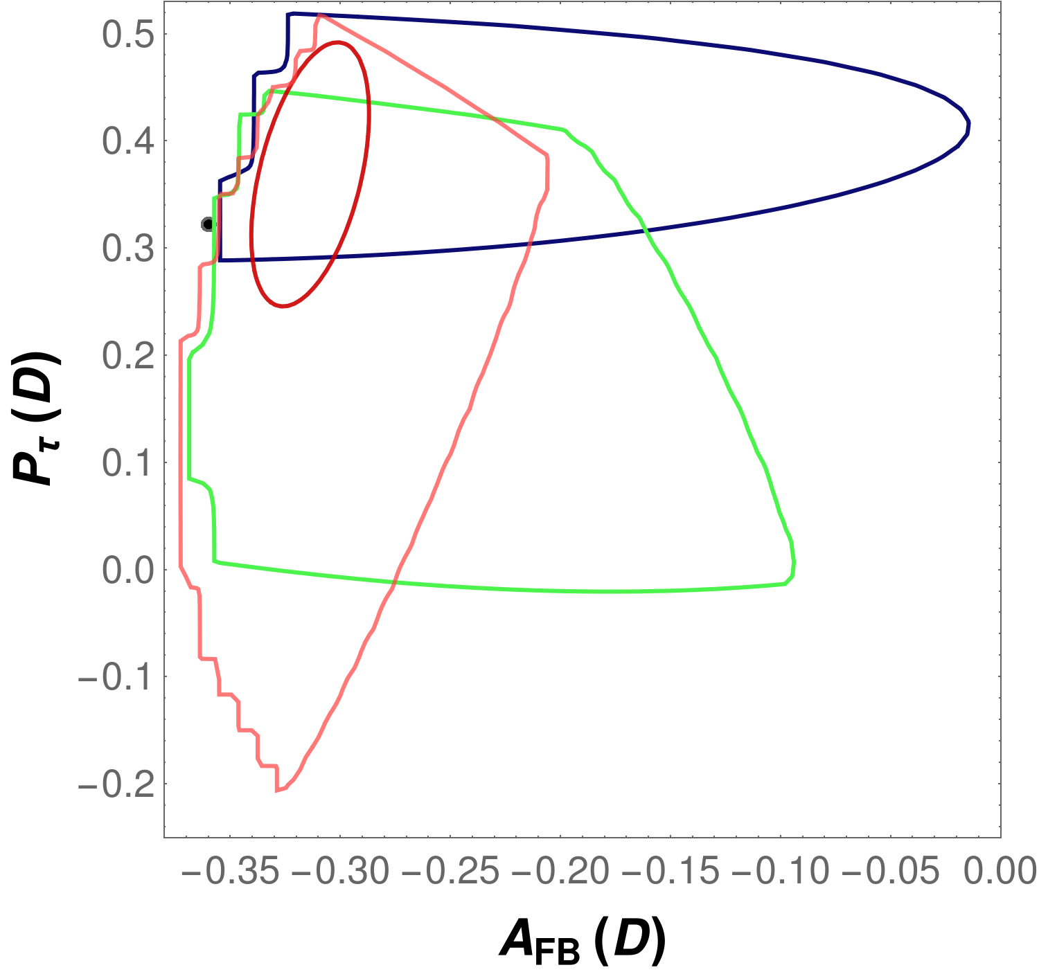
Figure 2: State-of-the-art fit results in single-mediator models for selected pairs of observables in $B\to D^{(*)}\tau\nu$ decays (following Ref. Murgui:2019czp for form factor and input treatment). All outer ellipses correspond to $95\%$ confidence level, inner (where present) to $68\%$. We show the SM prediction in grey, the experimental measurement/average in yellow (where applicable) and scenarios I, II, III IV and V in dark green, green, dark blue, dark red and red, respectively, see text. Contours outside the experimental ellispse imply that the measured central values cannot be accomodated within that scenario. The limit $BR(B_{c}\to\tau\nu)\leq 30\%$ has been applied throughout, but affects only the fits with scalar coefficients. Dark green contours are missing in the two graphs on the right, because the predictions of scenario I are identical to the SM ones.

In addition to the above observables, the leptonic decay $B_{c}\to\tau\nu$ plays a special role. Although it is not expected to be measured in the foreseeable future, it provides nevertheless a strong constraint on NP, since the relative influence of scalar NP is enhanced in this mode. A limit can then be obtained even from the total width of the $B_{c}$ meson Li:2016vvp . Theoretical estimates for the partial width assumed unaffected by NP can be used to strengthen these bounds Beneke:1996xe ; Alonso:2016oyd ; Celis:2016azn , and also data from LEP Akeroyd:2017mhr . Both approaches rely on additional assumptions, however, see Refs. Blanke:2018yud ; Bardhan:2019ljo for recent extensive discussions.

The constraints discussed so far are relevant in any scenario trying to address the existing anomalies. An interesting subclass of such models is that where the existence of a single mediator coupling to only the known SM degrees of freedom is assumed, classified in Freytsis:2015qca , creating only a subset of the possible operators at the $b$ scale. Among those, only five scenarios remain that can reasonably well accomodate the data described above, see also Refs. Tanaka:2012nw ; Blanke:2018yud ; Freytsis:2015qca ; Bhattacharya:2016zcw ; Ivanov:2017mrj ; Alok:2017qsi ; Bifani:2018zmi ; Blanke:2019qrx ; Shi:2019gxi for comparisons (additional constraints in specific scenarios are commented on below): Scenario I yields only a left-handed vector operator, created by either a heavy color-less vector particle Greljo:2015mma ; Boucenna:2016wpr ; Boucenna:2016qad ; Megias:2017ove (phenomenologically highly disfavored) or a leptoquark, see Refs. Li:2016vvp ; Fajfer:2012jt ; Deshpande:2012rr ; Sakaki:2013bfa ; Duraisamy:2014sna ; Calibbi:2015kma ; Fajfer:2015ycq ; Barbieri:2015yvd ; Alonso:2015sja ; Bauer:2015knc ; Das:2016vkr ; Deshpand:2016cpw ; Sahoo:2016pet ; Dumont:2016xpj ; Becirevic:2016yqi ; Barbieri:2016las ; DiLuzio:2017vat ; Assad:2017iib ; Chen:2017hir ; Bordone:2017bld ; Altmannshofer:2017poe ; Calibbi:2017qbu ; Becirevic:2018afm ; Fornal:2018dqn ; Blanke:2018sro ; Crivellin:2017zlb for this and other leptoquark variants. Scenario II includes Scenario I, but yields also a right-handed scalar operator, realized for example by a vector leptoquark. Scenario III involves both left- and right-handed scalar operators, generated for instance by a charged Higgs Crivellin:2012ye ; Celis:2012dk ; Crivellin:2015hha ; Celis:2016azn ; Chen:2017eby ; Iguro:2017ysu ; Chen:2018hqy ; Li:2018rax (with a limited capability to accomodate $R(D^{*})$ due to the $B_{c}$ constraint discussed above). Scenarios IV and V involve the left-handed scalar and tensor operator which are generated proportionally to each other ($C_{S_{L}}=\pm 4C_{T}$ at the NP scale $\Lambda$), in the latter case with the addition of the left-handed vector operator, again realized in leptoquark models. It is also possible to analyze the available data in more general contexts. For example, within SMEFT the right-handed vector current is expected to be universal Cirigliano:2009wk ; Alonso:2014csa ; Cata:2015lta , see Murgui:2019czp for a global analysis in this framework, while this does not hold when the electroweak symmetry breaking is realized non-linearly Cata:2015lta . Allowing for additional light degrees of freedom beyond the SM opens the possibility of contributions with right-handed neutrinos, see Refs. He:2012zp ; Becirevic:2016yqi ; He:2017bft ; Greljo:2018ogz ; Asadi:2018wea ; Robinson:2018gza ; Azatov:2018kzb ; Heeck:2018ntp .

Once specific models are considered, typically additional constraints apply. Important ones include high-$p_{T}$ searches, looking for collider signatures of the mediators related to the anomaly Faroughy:2016osc ; Feruglio:2018fxo ; Greljo:2018tzh ; Altmannshofer:2017yso , RGE-induced flavor-non-universal effects in $\tau$ decays Feruglio:2017rjo , lepton-flavor violating decays Feruglio:2017rjo , precision universality tests in quarkonia decays Aloni:2017eny , charged-lepton magnetic moments Feruglio:2018fxo and electric dipole moments in models with non-vanishing imaginary parts Dekens:2018bci .

2.7 Interpretation of experimental results

The reconstructed kinematic distributions used in measurements are sensitive to both the modeling of required non-perturbative inputs (e.g., form factors, light-cone meson wave functions), and to assumptions about the underlying fundamental theory (e.g. possible presence of operators with chiral structures different from those found in the SM). Current measurements assume the SM operator structure, and include the non-perturbative uncertainties as they are known at the time of publication. While this is a valid strategy for testing the SM, if in future the presence of a non-SM contribution with a different chiral structure is established then past measurements will require reinterpretation.

In order to present experimental results in such a way to allow a-posteriori analyses to have maximum flexibility in the description of non-perturbative inputs and BSM content, the following strategies might be considered. The techniques to allow for reinterpretation of results overlap with those used to make differential measurements designed to be sensitive to the chiral structure and non-perturbative quantities.

A first possibility, is the publication of unfolded distributions (see, for instance, the $B\to D^{*}\ell\nu$ spectrum presented in Ref. Abdesselam:2017kjf ). This method offers the possibility to fit with ease the experimental results to arbitrary parametrizations of the form factors Bigi:2017njr ; Grinstein:2017nlq ; Bernlochner:2017jka ; its downside is that it requires relatively high statistics and that the unfolded distributions do not contain the whole experimental information.

A second option, which has been employed in the untagged Belle analysis of ref. Waheed:2018djm , is to provide folded distributions in which detector effects are not removed and no extrapolation is performed, together with experimental efficiencies and the detector response matrix (which reproduces detector effects to a given accuracy). This allows the use of any parametrization of SM and BSM effects in comparing with the experimental result. This approach, while requiring slightly more involved a posteriori fitting strategies, avoids the statistical problems associated with unfolding and can be extended more easily to higher dimensions.

Finally, the most complete information is contained in the Likelihood function which depends on a set of SM parameters (e.g., for $B\to\pi\ell\nu$ they could be the coefficients of the $z$-expansion of the form factors and $V_{ub}$) and on the Wilson coefficients of BSM operators). This method has not been currently pursued in any $B$ decay measurement, in part because of difficulties related to the extremely large amount of information that would need to be presented. Two differing approaches are to publish the full experimental Likelihood in the full parameter space of BSM Wilson coefficients and SM non-perturbative coefficients, or to publish the tools for external readers to be able to repeat the full experimental fit with the signal model varied. For representing the experimental Likelihood in a high-dimensional space, possible approaches include the use of Markov chain sampling, or MVA surface modelling. These are the only strategies which would allow the entirety of the experimental information to be available in a posteriori theoretical investigations. It is essential to this approach for the experimental measurement to cover the full parameter space in a sufficiently general way, including alternative Likelihoods with different parametrizations for nonperturbative effects.

2.8 HAMMER

Future new physics searches in $b\to c\,\tau\nu_{\tau}$ decays are a challenging endeavor: most experimental results make use of kinematic properties of the process to discriminate between the signal of interests and backgrounds. For instance recent measurements from the $B$-factories BaBar and Belle used the lepton momentum spectrum and measurements of LHCb use fits to the four-momentum transfer $q^{2}$. In new physics scenarios, these distributions change and alter the analysis acceptance, efficiencies, and extracted signal yields. In addition, large samples of simulated decay processes play an integral part in those measurements. In most, one of the leading systematic uncertainties is due to the limited availability of such samples. Thus producing large enough simulation samples for a wide range of new physics points, needed to take into account the aforementioned changes in acceptance, etc. is not a viable path. This is where the tool HAMMER Bernlochner:2020tfi ; Duell:2016maj can help: it implements an event-level reweighting, assigning a weight based on the ratio of new physics to simulated matrix element, which allows one to re-use the already generated events. In addition, it is capable of providing histograms for arbitrary new-physics parameter values (including also form factor variations), which can be used, for example, in template fits to kinematic observables. These event weights can completely account for acceptance changes and will enable Belle II and LHCb to directly extract limits on the Wilson coefficients present in $b\to c\,\tau\nu$ transitions.

3 Heavy-to-light exclusive

In this section we present an overview of $b\to u$ exclusive decays. We start with a discussion of the lattice calculations of the $b$ hadron decay form factors to a light pseudoscalar, vector meson or baryon. We then review the light-cone sum rule calculation of the same form factors and the current experimental situation, as well as the prospects at Belle II and LHCb. Finally, we briefly discuss a few related subjects, such as the semitauonic heavy to light decays, the decay $b\to\gamma\ell\nu_{\ell}$, the non-resonant $B\to\pi\pi\ell\nu$ decays, and some subtlety of the $z$-expansion.

3.1 Form factors for semileptonic $b$-hadron decays into light hadrons from lattice QCD

3.1.1 Form factor parametrizations

The matrix elements that describe the hadronic part of the semileptonic transitions $B\to X\ell\nu$ or $B\to X\ell\ell$ are parametrized in terms of the form factors in Eqs. (1)–(3), where $X$ now denotes a pion or kaon. The transitions $B\to X^{*}\ell\nu$ or $B\to X^{*}\ell\ell$ are parametrized in terms of the form factors in Eqs. (4)–(7), where $X^{*}$ now denotes a $\rho$, $K^{*}$, or $\phi$ meson. As discussed in Sec. 2.1, modern theoretical calculations of the form factors employ $z$-parametrizations to describe their shapes, which can be implemented in a model-independent way, being based on analyticity and unitarity constraints. For the case at hand, an often used choice for the $z$-parameter defined in Eq. (9) is $t_{0}=(M+m)/(\sqrt{M}-\sqrt{m})^{2}$, which results in a range $|z|<0.3$, centered around $z=0$. In general, the small range of $z$ coupled with unitarity constraints on the coefficients ensure that the polynomial expansions converge quickly. As discussed already in Sec. 2.1, for $B$-meson decays to light hadrons with their larger $q^{2}$ range, the BCL parametrization Bourrely:2008za is the standard choice, as the resulting forms satisfy the expected asymptotic $q^{2}$ and near threshold scaling behaviors Lepage:1980fj ; Akhoury:1993uw :

$$f_{+}(q^{2}) = \frac{1}{1-q^{2}/M_{B^{*}(1^{-})}^{2}}\sum\limits_{n=0}^{N_{z}-1}b_{n}^{+}(t_{0})\left(z^{n}-(-1)^{n-N_{z}}\frac{n}{N_{z}}z^{N_{z}}\right),$$ (45)

$$f_{0}(q^{2}) = \frac{1}{1-q^{2}/M_{B^{*}(0^{+})}^{2}}\sum\limits_{n=0}^{N_{z}}b_{n}^{0}(t_{0})\,z^{n}.$$ (46)

3.1.2 Lattice QCD results for $B$-meson decay form factors to light pseudoscalars

Lattice-QCD calculations of the form factors for semileptonic $B_{(s)}$-meson decays to light hadrons proceed along the same lines as discussed in Sec. 2.2. In particular, there are a number of different, well-developed strategies for dealing with the heavy $b$-quark in lattice QCD, see Ref. Aoki:2019cca for a review. The same two- and three-point functions as for the heavy-to-heavy case are needed here, albeit with the appropriate valence quark propagators, to describe the heavy-to-light decay process. While this affects the statistical errors in the next step, the fits to the spectral representations of the correlation functions to obtain the desired matrix elements on each gauge ensemble and each recoil momentum, the procedure is essentially the same. The resulting “lattice data” are then used in combined chiral-continuum fits coupled with a systematic errors analysis to obtain the form factors in the continuum over the range of recoil energies that are included in the simulations. Here, a well known challenge is that the recoil energies that are accessible in lattice-QCD calculations cover only a fraction of the entire kinematic region. A related challenge is that the validity of Chiral Perturbation Theory (used to extrapolate or interpolate to the physical pion mass) is limited to pion energies of $\approx 1$ GeV. The final step is the $z$-expansion fit, from which the form factors are obtained over the entire kinematic range, albeit with larger errors in the region not directly covered in the lattice calculation.

Lattice-QCD calculations of the $B\to\pi$ vector current form factors $f_{+}$ and $f_{0}$ can be used to determine $|V_{ub}|$ from experimental measurements of the $B\to\pi\ell\nu$ decay rate. There are currently two independent, published lattice-QCD computations that employ the modern methods outlined above, including the model-independent $z$-expansion Flynn:2015mha ; Lattice:2015tia . The RBC/UKQCD collaboration Flynn:2015mha uses ensembles with $N_{f}=2+1$ flavors of Domain Wall fermions at two lattice spacings with sea-pion masses in the range $[300,400]$ MeV. The Fermilab/MILC collaboration Lattice:2015tia uses ensembles with $N_{f}=2+1$ flavors of asqtad (improved staggered) fermion at four lattice spacings covering the range $a\approx 0.045-0.12$ fm and a range of sea-pion masses down to $177$ MeV. Earlier work Bailey:2008wp used a subset of these ensembles. The treatment of the $b$-quark is similar in the two works; Ref. Flynn:2015mha uses a variant of the Fermilab approach, called the relativistic heavy quark (RHQ) action, while Ref. Lattice:2015tia employs the original Fermilab formalism. Both groups also use the mostly nonperturbative renormalization method to compute the renormalization factors. The form factors obtained by the two lattice groups are in good agreement with each other, and can be combined in joint fits together with experimental data for an improved $|V_{ub}|$ determination Aoki:2019cca .

Ongoing work by RBC/UKQCD is extending the calculation to include more ensembles Flynn:2019jbg . Ongoing work by the Fermilab/MILC collaboration employs the HISQ $N_{f}=2+1+1$ ensembles with sea-pion masses at (or near) the physical point, and the Fermilab formalism for the $b$-quark Gelzer:2019zwx . The HPQCD collaboration has published a calculation of the scalar form factor for the $B\to\pi$ transition at zero recoil $f_{0}(q^{2}_{\text{max}})$ on a subset of the $N_{f}=2+1+1$ HISQ ensembles and treating the $b$ -quark in NRQCD Colquhoun:2015mfa , which provides a nice test of the soft-pion theorem, but cannot be used in $|V_{ub}|$ determinations. Ongoing work includes a calculation of the $B\to\pi$ form factors over a range of $q^{2}$ on a subset of the asqtad ensembles using NRQCD $b$-quarks and HISQ light-valence quarks Bouchard:2013zda . The JLQCD collaboration has an ongoing project to calculate the $B\to\pi$ form factors on $N_{f}=2+1$ Domain Wall ensembles using also Domain Wall fermions for the heavy and light valence quarks Colquhoun:2019tyq . They focus their calculation on small lattice spacings ($a\approx 0.044-0.080$ fm) and include a series of heavy-quark masses to extrapolate to the physical $b$-quark mass.

The vector current form factors $f_{+}$ and $f_{0}$ needed for rare $B\to\pi\ell\ell$ decay are the same as for $B\to\pi\ell\nu$ decay (up to small isospin corrections), but the tensor form factor $f_{T}$ is also needed to describe the rare process in the SM, while it can contribute to $B\to\pi\ell\nu$ decay only in BSM theories. So far, $f_{T}$ has been calculated only by the Fermilab/MILC collaboration Bailey:2015nbd using the same ensembles and methods as for the vector current form factors. However, most (if not all) of the ongoing projects described above, now include the complete set of form factors in their analyses, and new results for this form factor will therefore also be forthcoming.

The $B_{s}\to K\ell\nu$ process can be used for an alternate determination of $|V_{ub}|$, and there currently are three independent, published lattice-QCD computations of the vector-current form factors Bouchard:2014ypa ; Flynn:2015mha ; Bazavov:2019aom . In Ref. Bouchard:2014ypa the HPQCD collaboration used NRQCD $b$-quarks and HISQ light-valence quarks to calculate the form factors on a subset of asqtad ensembles. The RBC/UKQCD Flynn:2015mha work is already described above, since they calculated the $B_{s}\to K$ and $B\to\pi$ transition form factors together. The Fermilab/MILC collaboration Bazavov:2019aom used the same methods and set-up as for their $B\to\pi$ project Lattice:2015tia but on a subset of asqtad ensembles. Both Fermilab/MILC Bazavov:2019aom and, in a follow-up paper, HPQCD Monahan:2018lzv also computed ratios of $B_{s}\to K$ and $B_{s}\to D_{s}$ observables, which can be used in combination with LHCb measurements to determine $|V_{ub}/V_{cb}|$.

3.1.3 Challenges of vector mesons

Lattice calculations of $B_{(s)}$ decay form factors with vector mesons ($\rho$, $K^{*}$, $\phi$) in the final state are substantially more challenging, as these vector mesons are unstable resonances for sufficiently light quark masses. The asymptotic final state in the continuum then contains (at least) two hadrons, and the relation with the finite-volume matrix elements computed on the lattice becomes nontrivial. The formalism that allows a mapping of finite-volume to infinite-volume $1\to 2$ hadron matrix elements has been developed Lellouch:2000pv ; Lin:2001ek ; Christ:2005gi ; Hansen:2012tf ; Briceno:2014uqa ; Briceno:2015csa ; Agadjanov:2016fbd and will be discussed in more detail below. First numerical applications to a form factor with nonzero momentum transfer have been published for the electromagnetic process $\pi\gamma^{*}\to\pi\pi$, where the $\pi\pi$ final state in a $P$ wave couples to the $\rho$ resonance Briceno:2015dca ; Briceno:2016kkp ; Alexandrou:2018jbt .

The lattice QCD calculations of $B_{(s)}\to V$ form factors published to date did not implement this $1\to 2$ formalism. For the $B\to\rho$ form factors, there is only an early study by the UKQCD collaboration Bowler:2004zb , performed in the quenched approximation and with heavy up and down quark masses for which the $\rho$ is stable. For the $B\to K^{*}$, $B_{s}\to K^{*}$, $B_{s}\to\phi$ form factors, an unquenched lattice QCD calculation is available Horgan:2013hoa . This work used three different ensembles of lattice gauge field configurations with pion masses of approximately 310, 340, and 520 MeV. For the lower two pion masses, the $K^{*}$ is expected to be unstable, but the analysis was performed as if the $K^{*}$ were stable. This entails using only a quark-antiquark interpolating field for the $K^{*}$, and assuming that the information extracted from exponential fits to the two-point and three-point correlation functions corresponds to the “$K^{*}$” contribution. The systematic errors introduced by this treatment are difficult to quantify. For unstable $K^{*}$, none of the actual discrete finite-volume energy levels directly corresponds to the resonance, and the actual ground state may be far from the resonance location (for typical lattice volumes, this problem is more severe at nonzero momentum). However, a quark-antiquark interpolating field couples more strongly to energy levels in the vicinity of the resonance, and ground-state saturation is typically not seen in the correlation functions before the statistical noise becomes overwhelming. In these cases, exponential fits are still dominated by one or multiple energy levels in the vicinity of the resonance.

In the following, we will denote the vector meson resonance as $V$, and the two pseudoscalar mesons whose scattering shows the resonance as $P_{1}$ and $P_{2}$. The finite-volume energy levels for a given total momentum and irreducible representation of the appropriate symmetry group are determined by the Lüscher quantization condition Luscher:1990ux and its generalizations, as reviewed in Ref. Briceno:2017max . In the absence of interactions, they would consist of $P_{1}P_{2}$ scattering states with energies equal to the sums of the $P_{1}$ and $P_{2}$ energies, where the $P_{1}$ and $P_{2}$ momenta take on the discrete values allowed by the periodic boundary conditions. Through the $P_{1}P_{2}$ interactions, these energy levels are shifted away from their noninteracting values in a volume-dependent way. In the simplest case (considering only elastic scattering and neglecting the partial-wave mixing induced by the finite volume), each interacting finite-volume energy level can be mapped to a corresponding value of the infinite-volume $P_{1}P_{2}$ scattering phase shift, or, equivalently, scattering amplitude; more complicated cases with coupled channels and partial-wave mixing can also be treated. The dependence of the scattering amplitude on the $P_{1}P_{2}$ invariant-mass-squared, $s$, can be described by a Breit-Wigner-type function. By analytically continuing the scattering amplitude to complex $s$, one finds poles on the second Riemann sheet at $s=(m_{V}\pm i\Gamma_{V}/2)^{2}$, where $\Gamma_{V}$ is the width of the resonance. This procedure has been applied successfully to the $\rho$, $K^{*}$, and other resonances (see Ref. Briceno:2017max for a review).

The $B_{(s)}\to V$ form factors correspond to the residues at the pole at $s=(m_{V}-i\Gamma_{V}/2)^{2}$ in the $B_{(s)}\to P_{1}P_{2}$ form factors, where the $P_{1}P_{2}$ final state is projected to the $\ell=1$ partial wave. These $B_{(s)}\to P_{1}P_{2}$ form factors are functions of $q^{2}$ and $s$. In the single-channel case, the lattice computation involves the following steps: (i) Determine the $P_{1}P_{2}$ finite-volume energy spectrum, and the $B_{(s)}\to P_{1}P_{2}$ finite-volume matrix elements both for the ground states and multiple excited states. (ii) Obtain the infinite-volume $P_{1}P_{2}$ scattering amplitude from the finite-volume energy spectrum using the Lüscher method, and fit a suitable parametrisation of the $s$-dependence to the data. (iii) Map the finite-volume $B_{(s)}\to P_{1}P_{2}$ matrix elements to infinite-volume $B_{(s)}\to P_{1}P_{2}$ matrix elements using the Lellouch-Lüscher factor, which depends on the energy-derivative of the scattering phase shift and a known finite-volume function.

The finite-volume formalism requires the center-of-mass energy $\sqrt{s}$ to be small enough so that no more than two particles can be produced by the scattering through the strong interaction (however, the total momentum of the $P_{1}P_{2}$ system can in principle be arbitrarily large). For example, in the case of the $B\to\pi\pi$ form factors, the formalism requires $\sqrt{s}\lesssim 4\,m_{\pi}$, which becomes more restrictive when performing the calculation at lighter quark masses. However, it is likely that the coupling to four pions has negligible effects even at somewhat higher values of $\sqrt{s}$, as needed to map out the $\rho$ resonance region when using physical quark masses.

3.1.4 $\Lambda_{b}\to p$ and $\Lambda_{b}\to\Lambda^{(*)}$ form factors from lattice QCD

The $\Lambda_{b}\to p$ form factors relevant for the decay $\Lambda_{b}\to p\mu^{-}\bar{\nu}$ have been computed in lattice QCD together with the $\Lambda_{b}\to\Lambda_{c}$ form factors Detmold:2015aaa ; some aspects of this work were already discussed in Sec. 2.2.2. The lattice data for $\Lambda_{b}\to p$ cover the kinematic range from $q^{2}\approx 15\>{\rm GeV}^{2}$ to near $q^{2}_{\rm max}\approx 22\>{\rm GeV}^{2}$, and consequently the predicted $\Lambda_{b}\to p\mu^{-}\bar{\nu}_{\mu}$ differential decay rate is most precise in this range. The integrated decay rates in the Standard Model were found to be

$$\frac{1}{|{V_{ub}}|^{2}}\Gamma(\Lambda_{b}\to p\>\mu^{-}\bar{\nu}_{\mu})=(25.7\pm 2.6_{\,\rm stat}\pm 4.6_{\,\rm syst})\>\>{\rm ps}^{-1}$$ (47)

and

$$\frac{1}{|{V_{ub}}|^{2}}\int_{15\>{\rm GeV}^{2}}^{q^{2}_{\rm max}}\frac{\mathrm{d}\Gamma(\Lambda_{b}\to p\>\mu^{-}\bar{\nu}_{\mu})}{\mathrm{d}q^{2}}\mathrm{d}q^{2}=(12.31\pm 0.76_{\,\rm stat}\pm 0.77_{\,\rm syst})\>\>{\rm ps}^{-1}.$$ (48)

The latter has a total uncertainty of 8.8% (corresponding to a 4.4% theory uncertainty in a $|V_{ub}|$ determination from this rate), and the ratio to the partially integrated $\Lambda_{b}\to\Lambda_{c}\mu^{-}\bar{\nu}$ decay rate (38) has a total uncertainty of 9.8%, corresponding to a 4.9% theory uncertainty in the determination of $|V_{ub}/V_{cb}|$ performed by LHCb Aaij:2015bfa , commensurate with the experimental uncertainty. The $\Lambda_{b}\to p$ form factors from Ref. Detmold:2015aaa can also be used to predict the Standard-Model value of the baryonic $b\to u\ell\bar{\nu}$ lepton-flavor-universality ratio,

$$\frac{\Gamma(\Lambda_{b}\to p\>\tau^{-}\bar{\nu}_{\tau})}{\Gamma(\Lambda_{b}\to p\>\mu^{-}\bar{\nu}_{\mu})}\>=\>0.689\>\pm\>0.058_{\,\rm stat}\>\pm\>0.064_{\,\rm syst}.$$ (49)

By increasing statistics, removing the partially quenched data sets (cf. Sec. 2.2.2), adding one ensemble with physical light-quark masses, and another ensemble with a third, finer lattice spacing, it will likely be possible to reduce the uncertainties in both the $\Lambda_{b}\to p$ and $\Lambda_{b}\to\Lambda_{c}$ form factors by a factor of 2 in the near future.

The same methods have also been used to compute the $\Lambda_{b}\to\Lambda$ Detmold:2016pkz , $\Lambda_{c}\to p$ Meinel:2017ggx , and $\Lambda_{c}\to\Lambda$ Meinel:2016dqj form factors with lattice QCD. The latter calculation already includes an ensemble with the physical pion mass, and gave results for the $\Lambda_{c}\to\Lambda e^{+}\nu_{e}$ and $\Lambda_{c}\to\Lambda\mu^{+}\nu_{\mu}$ branching fractions consistent with, and two times more precise than, the measurements performed recently by the BESIII Collaboration Ablikim:2015prg ; Ablikim:2016vqd . This is a valuable test of the lattice methods used to determine the heavy-baryon decay form factors.

A lattice-QCD calculation is also in progress for the $\Lambda_{b}\to\Lambda^{*}(1520)$ form factors (in the narrow-width approximation) Meinel:2016cxo , which are relevant for the rare decay $\Lambda_{b}\to\Lambda^{*}(\to p\,K)\mu^{+}\mu^{-}$. As with $\Lambda_{b}\to\Lambda_{c}^{*}$, discussed in Sec. 2.2.2, this initial calculation only reaches $q^{2}$ in the vicinity of $q^{2}_{\rm max}$.

3.2 Light-cone sum rules calculations of heavy-to-light form factors

QCD sum rules on the light cone (LCSR) is a non-perturbative method for calculating hadronic quantities Balitsky:1986st ; Balitsky:1989ry ; Chernyak:1990ag . It has been applied to obtain the form factors for $B$ decays (see the definitions in Section 2.1). The first LCSR calculations relevant for $V_{ub}$ were performed in 1997 when the next-to-leading order (NLO) twist-2 corrections to $f_{+}(q^{2})$ were calculated Khodjamirian:1997ub ; Bagan:1997bp . The leading order (LO) corrections up to twist-4 were calculated in Ref. Belyaev:1994zk . Since the LO twist-3 contribution was found to be large, further improvements were made by calculating the smaller NLO corrections Ball:2004ye . A more recent update where the $\overline{\rm MS}$ mass is used in place of the pole mass for $m_{b}$ can be found in Ref. Duplancic:2008zz ; Khodjamirian:2011ub for the $B\to\pi$ case and in Ref. Duplancic:2008tk for the $B_{s}\to K$ case. Here we will discuss a selection of the more recent LCSR calculations.

For $B\to\pi$, a NNLO ($O(\alpha_{s}^{2}\beta_{0})$) calculation of $f_{+}(0)$ was performed, with the result $f_{+}(0)=(0.262^{+0.020}_{-0.023})$ with uncertainties $\lesssim 9\%$ Bharucha:2012wy . This calculation tested the argument that radiative corrections to $f_{+}f_{B}$ and $f_{B}$ should cancel when both calculated in sum rules (the 2-loop contribution to $f_{B}$ in QCDSR is sizeable). It was found that despite $\sim 9\%$ $O(\alpha_{s}^{2}\beta_{0})$ change to $f_{B}$, the effect on $f_{+}(0)$ was only $\sim 2\%$.

More recently unitarity bounds and extrapolation were used to perform a Bayesian analysis of the form factor $f_{+}(q^{2})$ for $B\to\pi$ Imsong:2014oqa . Prior distributions were taken for inputs, a likelihood function was constructed based on fulfilling the sum rule for $m_{B}$ to $1\%$, and posterior distributions were obtained using Bayes’ theorem. The posterior distributions of the inputs differed only for $s_{0}$, which was pushed to higher values $s_{0}=41\pm 4$ GeV (mainly due to the choice of $m_{b}$). Finally the results were fit to the BCL parametrisation, finding a central value of $f_{+}(0)=0.31\pm 0.02$. Obtaining $f_{+}(q^{2})$ and the first two derivatives at 0 and 10 ${\rm GeV}^{2}$ has allowed the extrapolation to higher $q^{2}$ using improved unitarity bounds.

$V_{ub}$ can also be obtained from the channels $B\to\rho/\omega$, and updated LCSR results were made available in 2015 Straub:2015ica . The improvements in these results include: the computation of full twist-4 (+partial twist-5) 2-particle DA contribution to FFs, plus the determination of certain so-far unknown twist-5 DAs in the asymptotic limit; a discussion of the non-resonant background for vector meson final states; the determination and usage of updated hadronic matrix elements, specifically the decay constants; fits with full error correlation matrix for the $z$ expansion coefficients, as well as an interpolation to the most recent lattice computation. The result for $|V_{ub}|$ from $B\to\rho\ell\nu$ has comparable errors to the $B\to\pi$ determination. In general the $B\to V$ results agree with previous exclusive determinations and global fits within errors.

Future prospects for exclusive $V_{ub}$ from LCSR include extending the subset of NNLO corrections calculated both in $q^{2}$ and to include all NNLO twist 2 and 3 contributions. It would also be beneficial to perform a Bayesian uncertainty analysis of all $B\to P$,$D\to P$ LCSRs (along the lines of the aforementioned analysis for $B\to\pi$ Imsong:2014oqa ). Finally the measurement of $B_{s}\to K\ell\nu$ at LHCb/Belle II will allow an important complementary determination of $V_{ub}$ using results from Ref. Khodjamirian:2017fxg .

3.3 Measuring $|V_{ub}|$ exclusively and the prospects for Belle II

The most precise exclusive determinations of $|V_{ub}|$ will ultimately come from the most theoretically clean $b\to u\ell^{-}\bar{\nu}_{\ell}$ modes: $\bar{B}^{0}\to\pi^{+}\ell^{-}\bar{\nu_{\ell}}$, $\bar{B}^{0}_{s}\to K^{+}\ell^{-}\bar{\nu_{\ell}}$ and $\Lambda^{0}_{b}\to p\ell^{-}\bar{\nu_{\ell}}$, which involve ground state hadrons in the final state. The main challenge facing measurements of $|V_{ub}|$ from these modes is the large background from $b\to c\ell^{-}\bar{\nu}_{\ell}$ decays, which is O($|V_{cb}|^{2}/|V_{ub}|^{2})\approx 100$ more likely to occur. This background is difficult to separate from signal given the need to partially reconstruct the missing signal neutrino.

Several measurements of exclusive $\bar{B}^{0}\to\pi^{+}\ell^{-}\bar{\nu_{\ell}}$ decays were made at the $B$ factories CLEO, BaBar and Belle. These measurements fall in to two categories of tagged and untagged measurements, which exploit the unique $e^{-}e^{+}\rightarrow\Upsilon(4S)\rightarrow B\bar{B}$ topology and fully hermetic detector design of the $B$ factories. In tagged measurements Sibidanov:2013rkk the non-Signal $B$ meson in the event is first reconstructed in a number of hadronic modes before selecting the signal pion and lepton. Exploiting the known energies and momenta of the interacting $e^{+}e^{-}$ beams allows for neutrino 4-momentum, $p_{\nu}$ to be reconstructed and the signal to be extracted using the missing mass squared of the neutrino, $M^{2}=p^{2}_{\nu}$. In untagged measurements Ha:2010rf ; delAmoSanchez:2010af the signal pion and lepton are first selected with a tight selection to reduce background from $b\to c\ell^{-}\bar{\nu}_{\ell}$ decays. The neutrino is then reconstructed by inclusively reconstructing the other $B$ in the event as a sum of remaining tracks and photons. The beam constrained mass, $M_{bc}$, and beam energy difference  are used as fit variables to simultaneously extract the signal. While tagged measurements give a high purity and better $q^{2}$ resolution they suffer from a much lower efficiency resulting from the branching fractions and reconstruction efficiencies for tagged modes.

In both tagged and un-tagged measurements the exclusive $\bar{B}^{0}\to\pi^{+}\ell^{-}\bar{\nu_{\ell}}$ signal is fitted in bins of $q^{2}$ to determine the partial branching fraction in each bin. These measurements together with LQCD and LCSR predictions can be used as constraints to simultaneously fit the form factors of decays and determine the parameter $|V_{ub}|$. HFLAV performed a fit for $|V_{ub}|$ the $\bar{B}^{0}\to\pi^{+}\ell^{-}\bar{\nu_{\ell}}$ form factor, $f_{+}(q^{2})$, under a BCL parametrisation utilising BaBar and Belle tagged and untaggged datasets and state of the art theory predictions Amhis:2016xyh . This resulted in the most precise determination of $|V_{ub}|$ to date, $|V_{ub}|=3.67\pm 0.09(exp)\pm 0.12(theo)$, which has a total uncertainty of 4%.

Untagged and tagged measurements of $|V_{ub}|$ from $\bar{B}^{0}\to\pi^{+}\ell^{-}\bar{\nu_{\ell}}$ decays at Belle II will significantly improve the precision on $|V_{ub}|$. In order to project the reduction in uncertainty both tagged and untagged analyses were performed on simulated Belle II Monte Carlo. The expected uncertainty on $|V_{ub}|$ was determined for a given luminosity by extracting the partial branching fractions from pseudo-datasets generated from Monto Carlo expectations and fitting these together with LQCD predictions. With $50$ ab^-1 and future expected improvements in LQCD predictions the projected uncertainties on $|V_{ub}|$ from $\bar{B}^{0}\to\pi^{+}\ell^{-}\bar{\nu_{\ell}}$ decays were 1.7% (tagged) and 1.3% (untagged). The dominant systematic for the tagged analysis is the calibration of the tagging efficiency which is assumed irreducible at $1\%$ on $|V_{ub}|$. For the untagged analysis the dominant systematic uncertainty results from the uncertainty on the number of $B\bar{B}$ pairs which is assumed irreducible at $0.5\%$. Several systematics relating to the branch fractions and form factors of $b\to c\ell^{-}\bar{\nu}_{\ell}$ and $b\to u\ell^{-}\bar{\nu}_{\ell}$ decays are also considered irreducible in the untagged analysis given the lower purity than the tagged analysis.

3.4 Measuring $|V_{ub}|/|V_{cb}|$ at LHCb

All $b$-hadron species are accessible at hadron colliders thus opening to LHCb a wide possibility of $|V_{ub}|$ measurements from exclusive $b\to u$ transitions, while inclusive $|V_{ub}|$ measurements do not seem feasible at the moment. In proton-proton collision at high energy $b\bar{b}$ quark pairs are produced mainly from gluon splitting and hadronize independently, as a consequence $b$-hadrons have a wide continuum momentum spectrum and the reconstruction of semileptonic decays can not profit of the beam-energy constraints used at B-factories. However, thanks to the large boost acquired by the $b$-hadrons, the direction of the momentum can be well determined by the vector connecting the primary vertex of proton-proton interactions and the $b$-hadron decay vertex. By imposing the $b$-hadron mass constraint, the missing neutrino momentum can be calculated with a two-fold ambiguity. A small fraction of unphysical solutions arises from the imperfect reconstruction of vertices positions. The best way to choose between the two solutions depends on the specific decay mode under study. The choice can be optimized considering additional variables related to the decay kinematics by using linear regression algorithms Ciezarek:2016lqu .

The precise determination of an absolute branching fraction requires the precise knowledge of the total $b$-hadron production rate and of the experimental detection efficiency, which includes reconstruction, trigger and final states selection. To minimize the experimental uncertainty it is preferred to determine ratios of branching fractions, normalizing the $b$-hadron decay mode under study to a well-known $b$-hadron decay mode, that has as similar as possible decay topology. Choosing a decay of the same $b$-hadron removes the dependence on the production fraction of the specific $b$-hadron.

The first determination of $|V_{ub}|$ at LHCb was done with baryons, measuring the branching fractions for $\Lambda_{b}\to p\mu^{-}{\overline{\nu}}$ and $\Lambda_{b}^{0}\to\Lambda_{c}^{+}\mu^{-}{\overline{\nu}}$ decays Aaij:2015bfa . What is directly determined is the ratio of the CKM matrix elements

$$\frac{|V_{ub}|^{2}}{|V_{cb}|^{2}}=\frac{\mathcal{B}(\Lambda_{b}^{0}\to p\mu^{-}{\overline{\nu}})}{\mathcal{B}(\Lambda_{b}^{0}\to\Lambda_{c}^{+}\mu^{-}{\overline{\nu}})}\times R_{FF}$$

where $R_{FF}$ is the ratio of the relevant form factors, calculated using LQCD. The ratio represents a band in the $|V_{ub}|$ versus $|V_{cb}|$ plane and can be converted into a measurement of $|V_{ub}|$ using existing measurements of $|V_{cb}|$. Approximately 10% of $b$-hadrons produced at LHC are $\Lambda_{b}$ and a clean signal identification is possible imposing stringent proton identification requirements. The large background from $b$-hadron decays with additional charged tracks in the decay products is strongly reduced employing isolation criteria by means of multivariate machine-learning algorithms. The signal yields are determined from a $\chi^{2}$ fit to the B corrected mass distributions of $\Lambda_{b}^{0}\to p\mu^{-}{\overline{\nu}}$ and $\Lambda_{b}^{0}\to\Lambda_{c}^{+}\mu^{-}{\overline{\nu}}$ candidates. The corrected mass is defined as $m_{corr}=\sqrt{m_{h\mu}^{2}+p_{\perp}^{2}}+p_{\perp}$ where $p_{\perp}$ is the momentum of the hadron-$\mu$ pair transverse to the $\Lambda_{b}^{0}$ flight direction.

The LQCD form-factors that are used in the calculation of $|V_{ub}|$ Detmold:2015aaa are most precise in the kinematic region where $q^{2}$, the invariant mass squared of the leptonic system, is high. When the branching fractions of the $b\to u$ ($b\to c$) decays are integrated in the region $q^{2}>15(7)\text{GeV}^{2}$ the theory uncertainty on ${|V_{ub}|}/{|V_{cb}|}$ is 4.9%. This measurements, performed with Run 1 data, gives ${|V_{ub}|}/{|V_{cb}|}=0.83\pm 0.004$ (stat) $\pm 0.004$ (syst), consistent with previous exclusive measurements of the two CKM matrix elements.

A new measurement of this type is currently under study at LHCb. It uses $B_{s}^{0}\to K^{+}\mu^{-}{\overline{\nu}}$ decays whose branching fraction is predicted to be of the same order of magnitude of the $\Lambda_{b}^{0}\to p\mu^{-}{\overline{\nu}}$ one.

The signal selection is challenging due to the large background from partially reconstructed decays of all species of $b$-hadrons, but it can exploit the good efficiency and purity of kaon and muon identification provided by the LHCb detector, the separation of the $K\mu$ vertex from primary vertex and the already mentioned isolation tools. The chosen normalization mode $B_{s}^{0}\to D_{s}^{+}\mu^{-}{\overline{\nu}}$, $D_{s}^{+}\to K^{-}K^{+}\pi^{+}$ benefits of small uncertainty in the $D_{s}^{+}$ branching fraction. The good identification of this decay mode, despite the large feed-down from $B^{0}_{s}$ decays to excited $D_{s}$ mesons with un-reconstructed neutral particles, has been proven to be possible at LHCb with the measurement of $B_{s}^{0}$ lifetime Aaij:2017vqj .

Form factors for the $B_{s}^{0}$ mesons decays to $K$ and $D_{s}$ have been calculated with LQCD by several groups Bouchard:2014ypa ; Flynn:2015mha . The calculation are performed in the high $q^{2}$ region and extrapolated to the full region with BGL or BCL z-expansions. Different calculations agree at high $q^{2}$, but there is currently a disagreement in the $q^{2}=0$ extrapolated value. For $B_{s}^{0}\to K^{+}\mu^{-}{\overline{\nu}}$ in the low $q^{2}$ region (up to 12 GeV²) form factors calculated with LCSR are also available Khodjamirian:2017fxg . The uncertainties on the experimental measurement of the $B_{s}^{0}\to K^{+}\mu^{-}{\overline{\nu}}$ yield increase at high $q^{2}$ (low kaon momentum) due to the reduced efficiency and the larger background contamination. It is foreseen to perform the measurement in few $q^{2}$ bins so that the use of different calculations of form factors will be possible. Larger data samples, accumulated during the LHCb Upgrade period will allow a differential measurement in finer $q^{2}$ bins.

Purely leptonic $B^{-}\to\mu^{-}{\bar{\nu}}$ decays are not accessible at LHCb. An alternate way has been tested, searching for the decay $B^{-}\to\mu^{-}{\bar{\nu}}\mu^{+}\mu^{-}$ where an hard photon is irradiated from the initial state and materializes into two muons. This decay has the experimental advantage of the presence of additional particles in the final state and of a larger branching fraction, due to the removal of the helicity suppression. An upper limit on the branching fraction of $1.6\times 10^{-8}$ has been determined with $4.7~{}\text{fb}^{-1}$ of integrated luminosity Aaij:2018pKa , making it a possible candidate for a $|V_{ub}|$ measurement in the LHCb Upgrade period LHCbUpgrade2 .

3.5 Related issues

3.5.1 $R_{\pi}$

The experimental signature of $B\to\pi\tau\nu_{\tau}$ is challenging: low in rate due to CKM suppression, this final state can only be isolated from backgrounds using multivariate analysis techniques. Due to the pseudoscalar nature of the pion in the final state, an increased sensitivity to certain new physics models involving scalar exchange particles is expected and measurements of this branching fraction offer an orthogonal path to probe the anomalies observed in $R(D)$ and $R(D^{*})$. The first limit on the branching fraction using leptonic and one-prong $\tau$ decay modes was reported by Ref. Hamer:2015jsa . They reported

$$\mathcal{B}(B^{0}\to\pi^{-}\,\tau^{+}\,\nu_{\tau})<2.8\times 10^{-4}\quad\text{at 95\% CL}\,,$$ (50)

using a frequentist method. This result can be converted into a value of $R_{\pi}=\Gamma(B^{0}\to\pi^{-}\,\tau^{+}\,\nu_{\tau})/\Gamma(B^{0}\to\pi^{-}\,\ell^{+}\,\nu_{\tau})$ with $\ell=e,\mu$ of

$$R_{\pi}=1.05\pm 0.51\,,$$ (51)

which can in turn be compared to the SM prediction of Refs. Lattice:2015tia ; Bernlochner:2015mya of

$$R_{\pi}=0.641\pm 0.016\,.$$ (52)

Although the current precision is very limited, this result can already exclude the model parameter space of new physics models e.g. charged Higgs bosons, cf. Ref. Bernlochner:2015mya . Albeit a challenging signature, the final state with a charged pion has excellent prospects to be discovered in the large future Belle II data set. A naive extrapolation of Eq. 51 using assuming SM couplings results in evidence with 4 ab^-1 and discovery with 11 ab^-1 of integrated luminosity. The theoretical precision in $R_{\pi}$ will further increase with progress in lattice and with combined light lepton and lattice fits (the measured spectra can constrain the low $q^{2}$ region, which the lattice has difficulties in predicting reliably).

3.5.2 Experimental status and prospects of $B\to\ell\nu_{\ell}\gamma$

The experimental study of $B\to\ell\nu_{\ell}\gamma$ with $\ell=e,\mu$ is challenging and requires the clean laboratory of an $e^{+}\,e^{-}$ machinery: in such a setting the known initial state and the full reconstruction of the second $B$-meson produced in the collision provide the necessary constraint to successfully identify this signature. In addition, to not be overwhelmed with background, only photons at high energies ( $\approx 1$ GeV or larger) can be studied this way. The difficulties lie in the low efficiency of the reconstruction performance of the second $B$-meson, which have to happen in low branching fraction hadronic modes, and the still sizeable cross-feed from $B\to\pi^{0}\,\ell\bar{\nu}_{\ell}$ and $B\to\eta\,\ell\bar{\nu}_{\ell}$ decays. These two semileptonic processes produce very similar final states, namely $B\to\ell\nu_{\ell}\gamma\gamma$, but can be reduced by looking for a unassigned second high-energetic photon in the collision event under study. To separate $B\to\ell\nu_{\ell}\gamma$ from such decays successfully a fit to

$$m_{\nu}^{2}\simeq m_{\rm miss}^{2}=\left(p_{B_{\rm sig}}-p_{\ell}-p_{\gamma}\right)^{2}$$ (53)

can be carried out. Here $p_{\ell}$ and $p_{\gamma}$ denote the reconstructed four-vectors of the visible final states of $B\to\ell\nu_{\ell}\gamma$. The four-vector of the decaying signal $B$-meson, $p_{B_{\rm sig}}$, can be reconstructed using the information from the reconstructed tag-side $B$-meson. Correctly reconstructed signal decays peak at $m_{\nu}^{2}\approx 0$ GeV², whereas the dominant semileptonic decays are shifted to higher values due to the absence of the additional photon in the four-vector sum. The sensitivity can be further increased by explicitly reconstructing the semileptonic backgrounds and combine this information into a global analysis. This was the strategy pursuit by Ref. Gelb:2018end , which constrained the $\pi^{0}$ semileptonic background this way. The current experimental limit with a lower photon energy cut of $1$ GeV is

$$\Delta\mathcal{B}(B\to\ell\nu_{\ell}\gamma)<3.0\times 10^{-6}\quad\text{at 95\% CL}\,.$$ (54)

The above limit was determined using a flat Bayesian prior.

The discovery prospects for this decay at Belle II are excellent: the improved tracking capabilities, better calorimeter electronics, and the continuous development of modern tagging algorithms such as Ref. Keck:2018lcd will help improving the sensitivity. Extrapolating from the central value and uncertainty of the currently most precise limit of Eq. 54 of $\Delta\mathcal{B}(B\to\ell\nu_{\ell}\gamma)=\left(1.4\pm 1.1\right)\times 10^{-6}$, evidence should be possible with 5 ab^-1 and a discovery is possible with 50 ab^-1 Gelb:49050 . In principle, after discovery the value of $\left|V_{ub}\right|$ could be extracted from this decay as well, along with the first inverse momentum of the light-cone distribution amplitude, $\lambda_{B}$. An extrapolation from the current sensitivity is shown in Figure 3, based on the numbers from Ref. Gelb:49050 . The sensitivity for $\left|V_{ub}\right|$ will not be competitive with other methods (leptonic and semileptonic), but the achievable precision on $\lambda_{B}$ will help measurements and interpretations, which rely on our understanding of the light-cone distribution amplitude properties.

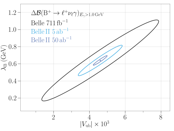
Figure 3: Projection of the extraction of $\lambda_{B}$ and $\left|V_{ub}\right|$ for the expected Belle II data sets. The ellipses correspond to the expected uncertainty. The figure is from Ref.Gelb:49050 .

3.5.3 Theoretical progress for $B\to\gamma\ell\nu_{\ell}$

The photoleptonic decay $B\to\gamma\ell\nu_{\ell}$ determined by two independent form factors is the simplest probe of the $B$-meson light-cone distribution amplitudes (LCDAs), which represent one of the most important inputs in the theory of semileptonic and nonleptonic $B$-decays based on QCD factorization and LCSRs. The calculation of the form factors in HQET and at large photon recoil in the leading power is well developed and can be found in Ref. Beneke:2011nf . The $1/m_{b}$ and $1/E_{\gamma}$ power suppresed effects, expressed in a form of the soft overlap part of the form factors, were quantified using a technique Braun:2012kp based on dispersion relations and quark-hadron duality (see also Ref. Wang:2016qii ). The most advanced calculation of the $B\to\gamma\ell\nu_{\ell}$ form factors, including power suppressed terms, was done recently Beneke:2018wjp resulting in the prediction of the decay branching fraction at $E_{\gamma}>1.0$ GeV as a function of the key unknown theoretical quantity: the inverse moment $\lambda_{B}$ of the B-meson LCDA. An alternative approach Wang:2018wfj calculates the power-suppressed corrections due to photon emission at long distances in terms of the photon LCDAs in the LCSR framework. The proof of concept for a lattice QCD calculation of radiative leptonic decays was recently done in Kane:2019jtj , see also deDivitiis:2019uzm .

3.5.4 $B\to\pi\pi\ell\nu_{\ell}$ decay beyond $\rho$

Calculations of $B\to\rho$ form factors both in lattice QCD and from LCSRs usually adopt a narrow $\rho$ approximation and by default ignore the influence of nonresonant effects (radially excited $\rho$’s) in the mass interval around $\rho$. The role of these effects has to be assessed at a quantitative level. In Refs. Hambrock:2015aor ; Cheng:2017sfk the first attempt to calculate more general $B\to\pi\pi$ form factors from LCSRs, using two-pion LCDAs at low mass of dipion system and at large recoil, was undertaken. The currently limited knowledge of these nonperturbative inputs calls for their further development and also for alternative methods. In Ref. Cheng:2017smj a different version of LCSRs with $B$ meson LCDAs was obtained which predicts the convolutions of the $\bar{B}^{0}\to\pi^{+}\pi^{0}$ form factors in $P$ wave with the timelike pion form factor. In the narrow $\rho$-meson limit these sum rules reproduce analytically the known LCSRs for $B\to\rho$ form factors. Using data for the pion vector form factor from $\tau$ decay, the finite-width effects and the contribution of excited $\rho$-resonances to the $B\to\pi\pi$ form factors were found to amount up to $\sim 20\%$ in the small dipion mass region where they can be interpreted as a nonresonant ($P$-wave) background to the $B\to\rho$ transition. For a more general analysis of $B\to\pi\pi\ell\nu_{\ell}$ decays see e.g. Refs. Faller:2013dwa ; Kang:2013jaa .

3.5.5 Remarks on the $z$ expansion

The use of the so-called $z$ expansion for form factors has become a standard practice for semileptonic decays, see Refs. Boyd:1997qw ; Hill:2006ub for a pedagogical discussion. In the workshop several issues concerning it were discussed, in particular its application to baryon form factors.

Form factors which parametrize matrix elements of the form $\langle L|J|H\rangle$ have known analytic structure. In particular, they are analytic in the complex $t=q^{2}$ plane outside a cut on the real axis. The cut starts at some positive $t_{\text{cut}}$ equals to the invariant mass squared of the lightest state the current $J$ can produce. The domain of analyticity can be mapped onto the unit circle via $z=\left(\sqrt{t_{\text{cut}}-t}-\sqrt{t_{\text{cut}}-t_{0}}\right)/\left(\sqrt{t_{\text{cut}}-t}+\sqrt{t_{\text{cut}}-t_{0}}\right)$, where $t_{0}$ is a free parameter denoting the point that is mapped to $z=0$. The form factor can be expanded as a Taylor series in $z$ which is a model-independent parametrization. For heavy-to-light form factors the maximum value of $z$ is related to the distance between $(m_{H}-m_{L})^{2}$ and $t_{\text{cut}}$. As a result, increasing $t_{\text{cut}}$ decreases the maximum value of $z$ leading to a faster convergence of the series.

Naively one might assume that the lightest state is the two-particle state $\bar{H}L$. This would imply that $t_{\text{cut}}=(m_{H}+m_{L})^{2}$, but this is not the case in general. For example, for the proton electric and magnetic form factors $(H=L=p)$ the cut starts at the two-pion threshold and not at the $p\bar{p}$ threshold. As another example, for one of the $B\to\pi$ form factors ($f_{+})$ the cut starts at $m^{2}_{B^{*}}$. Since this is a simple pole, it can be easily “removed” by considering $(t-m_{B^{*}})f_{+}$ as a Taylor series in $z$. For $(t-m_{B^{*}})f_{+}$ the cut starts at $(m_{B}+m_{\pi})^{2}$. If one uses a higher value of $t_{\text{cut}}$ than the physical one, one faces the danger of trying to expand the form factor in a region where it is not analytic. One of the immediate results of the workshop was the identification of such a problem in the literature. For baryon form factors, e.g. $\Lambda_{B}\to p$, analyses have used the wrong value of $t_{\text{cut}}=(m_{\Lambda_{B}}+m_{p})^{2}$, see Ref. Khodjamirian:2011jp and arXiv.org version 2 of Ref. Detmold:2015aaa . In fact, $t_{\text{cut}}$ for the baryon form factors is the same as for the meson form factors of analogous decays.

Another issue discussed in the workshop is the use (or lack of use) of bounds on the coefficients of the $z$ expansion. Although the form factor is expressed as an infinite series, in practice the series is truncated after a few terms. One would like to ensure that the value of a physical parameter such as $|V_{ub}|$ is independent of the number of parameters used, by bounding the coefficients. For example, one can use a unitarity bound Bourrely:1980gp or a bound from the heavy quark expansion Becher:2005bg . It seems that currently there is no consistent use of bounds in the extraction of $|V_{ub}|$. As the analysis Hill:2010yb shows, this can be a problem as the data improve and the number of necessary parameters increases. This can be especially problematic if one needs to use the $z$-expansion for extrapolation. The community needs to be aware of this issue and at least test that results do not change if bounds are applied to the coefficients.

The unitarity bounds for meson decays such as $B\to\pi$ rely on the fact that for $(t-m_{B^{*}})f_{+}$ the cut starts at the $(m_{B}+m_{\pi})^{2}$. For baryon decays such as $\Lambda_{B}\to p$, unitarity can only constrain the region above $(m_{\Lambda_{B}}+m_{p})^{2}$. The region between $(m_{B}+m_{\pi})^{2}$ and $(m_{\Lambda_{B}}+m_{p})^{2}$ is left unconstrained. Following the analysis of Ref. Hill:2010yb , one might worry that the contribution of the latter region is the dominant one. While considering together mesons and baryons contributions to the dispersive bounds might overcome the problem Cohen:2019zev , further study is warranted.

4 Quark masses and leptonic decays

4.1 Quark masses

In the Standard Model (and many extensions), quark masses and the CKM matrix all stem from Higgs-Yukawa couplings between the quark fields and the Higgs doublet. It is therefore natural to consider the bottom-quark mass, $m_{b}$, in this report. As discussed in Sec. 5, $m_{b}$ can be extracted from the inclusive semileptonic $B$ decay distributions, along with $|V_{cb}|$. In the theory of inclusive decays, the charm-quark mass, $m_{c}$, is also needed to control an infrared sensitivity; see Sec. 5.

Figure 4 compares results from lattice QCD with realistic sea content of $n_{f}=2+1+1$ or $2+1$ sea quarks with the FLAG 2019 Aoki:2019cca average for the $2+1+1$ sea.

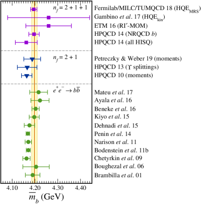
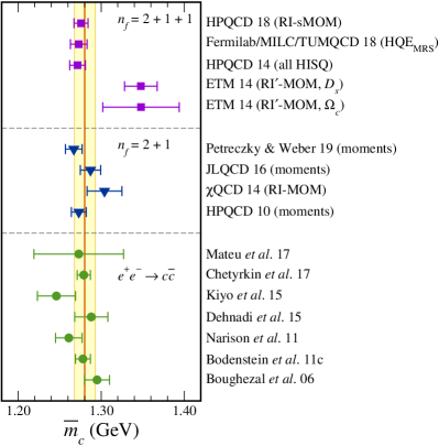
Figure 4: Comparison of results for the bottom-quark mass $\bar{m}_{b}=m_{b,\overline{\rm MS}}(m_{b,\overline{\rm MS}})$ (left) and the charm-quark mass $\bar{m}_{c}=m_{c,\overline{\rm MS}}(m_{c,\overline{\rm MS}})$ (right). Squares denote lattice-QCD calculations with $2+1+1$ flavors of sea quark Lytle:2018evc ; Bazavov:2018omf ; Gambino:2017vkx ; Bussone:2016iua ; Colquhoun:2014ica ; Chakraborty:2014aca ; Alexandrou:2014sha ; Carrasco:2014cwa ; triangles denote lattice-QCD calculations with $2+1$ flavors of sea quark Petreczky:2019ozv ; Nakayama:2016atf ; Yang:2014sea ; Lee:2013mla ; McNeile:2010ji ; circles denote results extracted from $e^{+}e^{-}$ collisions near $Q\bar{Q}$ threshold Mateu:2017hlz ; Chetyrkin:2017lif ; Ayala:2016sdn ; Beneke:2016oox ; Kiyo:2015ufa ; Dehnadi:2015fra ; Penin:2014zaa ; Narison:2011xe ; Bodenstein:2011fv ; Bodenstein:2011ma ; Chetyrkin:2009fv ; Boughezal:2006px ; Brambilla:2001qk . The vertical band shows the FLAG 2019 average for $2+1+1$ sea flavors. Note that $2+1$-flavor calculations are in rough (good) agreement for bottom (charm).

The average for $\bar{m}_{b}$ is dominated by the very precise result from the Fermilab Lattice, MILC, and TUMQCD Collaborations, while that for $\bar{m}_{c}$ is dominated by the corresponding Fermilab/MILC/TUMQCD result together with two separate results from the HPQCD Collaboration. The FLAG 2019 Aoki:2019cca averages (for $2+1+1$ sea flavors) are

$$\bar{m}_{b}=m_{b,\overline{\rm MS}}(m_{b,\overline{\rm MS}}) = 4.198(12)~{}\text{GeV},$$ (55)

$$\bar{m}_{c}=m_{c,\overline{\rm MS}}(m_{c,\overline{\rm MS}}) = 1.280(13)~{}\text{GeV},$$ (56)

based on Refs. Bazavov:2018omf ; Gambino:2017vkx ; Bussone:2016iua ; Colquhoun:2014ica ; Chakraborty:2014aca and Lytle:2018evc ; Bazavov:2018omf ; Chakraborty:2014aca ; Alexandrou:2014sha ; Carrasco:2014cwa , respectively. Another recent review Komijani:2020kst finds averages with somewhat smaller uncertainties

$$\bar{m}_{b}=m_{b,\overline{\rm MS}}(m_{b,\overline{\rm MS}}) = 4.188(10)~{}\text{GeV},$$ (57)

$$\bar{m}_{c}=m_{c,\overline{\rm MS}}(m_{c,\overline{\rm MS}}) = 1.2735(35)~{}\text{GeV},$$ (58)

based on the same original sources. In the case of $\bar{m}_{c}$, two results Alexandrou:2014sha ; Carrasco:2014cwa agree poorly with the others, increasing $\chi^{2}/\text{dof}$ of the average by a factor of around 5. FLAG 2019 Aoki:2019cca stretches the error bar by $\sqrt{\chi^{2}/\text{dof}}$, while Ref. Komijani:2020kst discards them: the resulting error bar is smaller because of the compatibility of the inputs as well as the lack of stretching. Other differences in averaging methodology are quantitatively unimportant. In either case, the quoted averages are much more precise than those in the PDG.

A last remark is that the most precise results Lytle:2018evc ; Bazavov:2018omf ; Chakraborty:2014aca all use the very high statistics MILC HISQ ensembles with staggered fermions for the sea quarks Bazavov:2012xda ; Bazavov:2017lyh . In the future, other groups Baron:2010bv ; Baron:2010th ; Aoki:2010dy ; Boyle:2017jwu will have to collect similar statistics to enable a complete cross check.

Four distinct methods are used in the results shown in Fig. 4: 1) converting the bare lattice mass to the $\overline{\rm MS}$ scheme, 2) fitting to a formula for the heavy-light hadron mass in the heavy-quark expansion Kronfeld:2000ck ; Kronfeld:2000gk , and 3) computing moments of quarkonium correlation functions Bochkarev:1995ai ; Allison:2008xk . The first two require an intermediate renormalization scheme that can be defined for any ultraviolet regulator: quark masses defined this way can be computed with lattice gauge theory or dimensional regularization. For example, HPQCD 13 ($\Upsilon$ decays) Lee:2013mla uses two-loop lattice perturbation theory to convert the bare NRQCD mass to the pole mass Hart:2004bd ; Hart:2009nr , and dimensional regularization to convert the pole mass into the $\overline{\rm MS}$ mass.

Instead of the pole mass, one can use a regularization-independent momentum-subtracted mass Martinelli:1994ty . Like the $\overline{\rm MS}$ scheme these RI-MOM schemes are mass-independent renormalization schemes, but they depend on the gauge. In lattice gauge theory, Landau gauge is easily obtained on each gauge-field configuration via a minimization procedure Davies:1987vs . The mass renormalization factor, $Z_{m}$, can be computed from the three point function for the scalar or pseudoscalar density, because $Z_{m}^{-1}=Z_{S}=Z_{P}$ (up to technical details for Wilson fermions). For example, the matrix element $\langle p^{\prime}|P|p\rangle$, between gauge-fixed quark states, can be used to define $Z_{P}$ using the same formulas for lattice gauge theory as for continuum gauge theory (with dimensional regularization) Martinelli:1994ty . The schemes labeled RI-MOM and RI^′-MOM use $p^{\prime}=p$ and slightly different definitions of the quark-field normalization $Z_{2}$; for a review see Ref. Aoki:2010yq . The momentum transfer $q\equiv p^{\prime}-p=0$ here, namely it is “exceptional” in the sense of Weinberg’s theorem Weinberg:1959nj . On the other hand, the RI-sMOM scheme Sturm:2009kb chooses $p^{\prime}$ and $p$ such that $p^{2}=q^{2}=p^{\prime 2}\equiv\mu^{2}$. Without the exceptional momentum, the extraction of $Z_{P}$ is more robust. It would be interesting to see whether RI-sMOM on the ETM 2+1+1 ensembles yields $\bar{m}_{b}$ favoring the RI^′-MOM results or the RI-sMOM results on MILC’s ensembles.

The HQE method starts with the HQE formula for a heavy-light hadron mass Falk:1992wt ; Bigi:1994ga ,

$$M=m+\bar{\Lambda}+\frac{\mu_{\pi}^{2}}{2m}-d_{J}\frac{\mu_{G}^{2}(m)}{2m}+\cdots,$$ (59)

where $M$ is the hadron mass, which is computed in lattice QCD as a function of the quark mass, $m$, and $d_{J}$ depends on the spin of the hadron. The quantities can be identified with the energy of gluons and light quarks, $\bar{\Lambda}$, the Fermi motion of the heavy quark, $\mu_{\pi}^{2}$, and the hyperfine splitting, $\mu_{G}^{2}$. ($\mu_{G}^{2}$ depends logarithmically on $m$.) Although this idea is not new Kronfeld:2000ck ; Kronfeld:2000gk , to be precise one has to confront the definition of $m$. Although the pole mass is natural in the context of the HQE, it is not suitable in practice, because of its infrared sensitivity. The $\overline{\rm MS}$ mass, on the other hand, breaks the power counting: $m_{\text{pole}}-m_{\overline{\rm MS}}\propto\alpha_{s}m_{\text{pole}}$. Instead, one chooses mass definitions that, in some sense, lie in between these two choices. Gambino et al. Gambino:2017vkx choose the kinetic mass Bigi:1996si , while Fermilab/MILC/TUMQCD Bazavov:2018omf choose the minimal renormalon subtracted (MRS) mass Brambilla:2017hcq . After extracting $m_{\text{kin}}$ or $m_{\text{MRS}}$ from fitting Eq. (59), the result can be converted to the $\overline{\rm MS}$ scheme with three- and four-loop perturbation theory, respectively. In addition to the different matching, the error bar from Fermilab/MILC/TUMQCD is so small because it is based on the largest data set of all calculations in Fig. 4. See Sec. 5.3 for further discussion and results for $\bar{\Lambda}$, $\mu_{\pi}^{2}$, $\mu_{G}^{2}$, and higher-dimension corrections to the HQE.

One can avoid an intermediate scheme by computing a short-distance quantity in lattice QCD, taking the continuum limit, and analyzing the result with $\overline{\rm MS}$ perturbation theory. For example, on can compute moments of quarkonium correlation functions Bochkarev:1995ai ; Allison:2008xk ,

$$G_{\Gamma}^{(n)} = \sum_{t}t^{n}G_{\Gamma}(t),$$ (60)

$$G_{\Gamma}(t) = c_{\Gamma}\sum_{\bm{x}}\langle\bar{Q}\Gamma Q(\bm{x},t)\,\bar{Q}\Gamma Q(\bm{0},0)\rangle,$$ (61)

for some Dirac matrix $\Gamma$. In lattice gauge theory, the pseudoscalar density needs no renormalization if $\Gamma=\gamma^{5}$ and $c_{\gamma^{5}}=m_{Q}^{2}$. The moments $G_{\Gamma}^{(n)}$ are physical observables with a good continuum limit, which is proportional to $m_{Q}$ to the appropriate power, multiplied by a dimensionless function of $\alpha_{s}(m_{Q})$. Thus, these moments also yield determinations of the strong coupling as well as quark masses. In Fig. 4, results obtained in this way are labeled “moments”.

The same moments $G_{\Gamma}^{(n)}$ can be obtained from the cross section for $e^{+}e^{-}$ annihilation into ${Q\bar{Q}}$ hadrons via a suitably subtracted dispersion relation. In this case, $\Gamma=\gamma^{\mu}$ for the electromagnetic current, and $c_{\gamma^{\mu}}=1$ because the electromagnetic current is conserved. Thus, the same perturbative calculations (only changing $\Gamma$) can be used to extract the bottom- and charm-quark masses and $\alpha_{s}$ from experimental measurements. The dispersion relation, related sum rules, and the perturbative series for the moments are the basis of the result labeled $e^{+}e^{-}\to{}b\bar{b}$ and $e^{+}e^{-}\to{}c\bar{c}$ in Fig. 4. The order $\alpha_{s}^{p}$, $p=1$, $2$, $3$, became available in 1993 Broadhurst:1993mw , 1997 Chetyrkin:1997mb , and 2006 Chetyrkin:2006xg ; Boughezal:2006px , respectively.

4.2 Leptonic decays

Instead of semileptonic decays, CKM matrix elements can also be determined from purely leptonic decays. For example, a goal of Belle II is to improve the determination of $V_{ub}$ from $B^{+}\to\tau^{+}\nu$, as well as $V_{cd}$ from $D^{+}\to\ell^{+}\nu$ and $V_{cs}$ from $D_{s}^{+}\to\ell^{+}\nu$, and a goal of LHCb is to observe $B_{c}\to\tau\nu$. The rates for leptonic decays suffer a helicity suppression, making tauonic and muonic decays preferred experimentally. Leptonic decays are mediated by the axial-vector part of the electroweak current, as well as possible pseudoscalar currents, so they complement semileptonic decays in this way.

The hadronic quantity describing the decay is known as the decay constant, defined by

$$\langle 0|\bar{b}\gamma^{\mu}\gamma^{5}u|B^{+}(p)\rangle=ip^{\mu}f_{B^{+}},$$ (62)

where $p^{\mu}$ is the four-momentum of the $B$ meson and $f_{B^{+}}$ is the decay constant. For other mesons, the axial currents and notation change in obvious ways. From the partial conservation of the flavor-nonsinglet axial current, the pseudoscalar density can also be used to compute the decay constant:

$$(m_{b}+m_{u})\langle 0|\bar{b}\gamma^{5}u|B^{+}(p)\rangle=M_{B^{+}}^{2}f_{B^{+}},$$ (63)

where $m_{b}$ and $m_{u}$ are bare quark masses.

Equations (62) and (63) are the basis of lattice-QCD calculations. In general, the axial current used is not a Noether current, so it is not absolutely normalized. Fermion formulations with good chiral symmetry (staggered, overlap, domain wall) provide an absolutely normalized pseudoscalar density. Until recently, however, lattice spacings have not been small enough to use these approaches for the $b$ quark. Methods developed especially for heavy quarks have therefore been used, and they do not provide any absolutely normalized $\bar{b}\Gamma u$ bilinears.

Figure 5 compares results from lattice QCD with realistic sea content of $n_{f}=2+1+1$ or $2+1$ sea quarks with the FLAG 2019 Aoki:2019cca average for the $2+1+1$ sea.

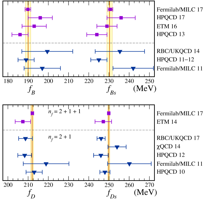
Figure 5: Comparison of results for the $B_{(s)}$-meson (top) and the $D_{(s)}$-meson (bottom) decay constants. Squares denote lattice-QCD calculations with $2+1+1$ flavors of sea quark Bazavov:2017lyh ; Hughes:2017spc ; Bussone:2016iua ; Carrasco:2014poa ; Dowdall:2013tga ; triangles denote lattice-QCD calculations with $2+1$ flavors of sea quark Boyle:2017jwu ; Christ:2014uea ; Yang:2014sea ; Na:2012iu ; Na:2012kp ; McNeile:2011ng ; Bazavov:2011aa ; Davies:2010ip . The vertical bands show the FLAG 2019 average for $2+1+1$ sea flavors Aoki:2019cca .

Because the Fermilab/MILC results dominate the FLAG average, we simply quote them Bazavov:2017lyh :

$$f_{B^{+}} = 189.4(0.8)_{\text{stat}}(1.1)_{\text{syst}}(0.3)_{f_{\pi,\rm PDG}}[0.1]_{\text{EM scheme}}~{}\text{MeV},$$ (64)

$$f_{B^{0}} = 190.5(0.8)_{\text{stat}}(1.0)_{\text{syst}}(0.3)_{f_{\pi,\rm PDG}}[0.1]_{\text{EM scheme}}~{}\text{MeV},$$ (65)

$$f_{B_{s}} = 230.7(0.8)_{\text{stat}}(1.0)_{\text{syst}}(0.2)_{f_{\pi,\rm PDG}}[0.2]_{\text{EM scheme}}~{}\text{MeV}.$$ (66)

$$f_{D^{0}} = 211.6(0.3)_{\text{stat}}(0.5)_{\text{syst}}(0.2)_{f_{\pi,\rm PDG}}[0.2]_{\text{EM scheme}}~{}\text{MeV},$$ (67)

$$f_{D^{+}} = 212.7(0.3)_{\text{stat}}(0.4)_{\text{syst}}(0.2)_{f_{\pi,\rm PDG}}[0.2]_{\text{EM scheme}}~{}\text{MeV},$$ (68)

$$f_{D_{s}} = 249.9(0.3)_{\text{stat}}(0.2)_{\text{syst}}(0.2)_{f_{\pi,\rm PDG}}[0.2]_{\text{EM scheme}}~{}\text{MeV},$$ (69)

where the systematic uncertainties stem from different choices in choosing fit ranges for the correlation functions and checking the continuum extrapolation by adding a coarser lattice; the third “$f_{\pi,\rm PDG}$” error comes from converting from lattice units to MeV with the pion decay constant of the PDG PDG2018 ; the last uncertainty stems from ambiguities in estimating electromagnetic effects in the context of a QCD calculation omitting QED. The results are arguably precise enough for the foreseeable future.

The results in Eqs. (64)–(69) again use the very high statistics MILC HISQ ensembles with staggered fermions for the sea quarks. Here the lattice spacing is, for some ensembles, small enough to reach the $b$ quark, so the calculation uses the HISQ action for all $b$ and light quarks alike. Thus, an absolutely normalized pseudoscalar density is available, so the uncertainty is essentially statistical, as propagated through a fit to the continuum limit with physical quark mass. Again, other groups will have to collect similar statistics in the future to enable a complete cross check.

To go beyond the precision quoted here, analyses of leptonic decays will have to include QED radiative corrections to the measured rates. The issues and an elegant solution for light mesons (pion and kaon) can be found in Refs. Carrasco:2015xwa ; Giusti:2017dwk ; DiCarlo:2019thl . Radiative corrections for heavy-light mesons will be more difficult to incorporate, because of the hierarchy of soft scales $\Lambda_{\text{QCD}}$, $\Lambda_{\text{QCD}}^{2}/m_{Q}$, $\Lambda_{\text{QCD}}^{3}/m_{Q}^{2}$, etc.

5 Heavy-to-heavy inclusive

5.1 Heavy Quark Expansion for $b\to c$

5.1.1 Review of the Current Status

The heavy quark expansion (HQE) for the inclusive semileptonic $b\to c$ transitions starts form a correlation function for the $b\to c$ current

$$d\Gamma\propto\sum_{X}(2\pi)^{4}\delta^{4}(P_{B}-P_{X}-q)\langle B(v)|\bar{b}\gamma_{\mu}(1-\gamma_{5})c|X\rangle\,\langle X|\bar{c}\gamma_{\nu}(1-\gamma_{5})b|B(v)\rangle$$

$$=\int d^{4}x\,e^{iq\cdot x}\,\langle B(v)|\bar{b}(x)\gamma_{\mu}(1-\gamma_{5})c(x)\bar{c}\gamma_{\nu}(1-\gamma_{5})b|B(v)\rangle$$

$$=2\mbox{ Im}\int d^{4}x\,e^{iq\cdot x}\,\langle B(v)|T\{\bar{b}(x)\gamma_{\mu}(1-\gamma_{5})c(x)\bar{c}\gamma_{\nu}(1-\gamma_{5})b\}|B(v)\rangle$$ (70)

$$=2\mbox{ Im}\int d^{4}x\,e^{-i(m_{b}v-q)\cdot x}\langle B(v)|T\{\bar{b}_{v}(x)\gamma_{\mu}(1-\gamma_{5})c(x)\bar{c}\gamma_{\nu}(1-\gamma_{5})b_{v}\}|B(v)\rangle$$

with

$$b(x)=e^{-im_{b}v\cdot x}b_{v}(x)\,.$$

The time ordered product in the last line can be expanded in an operator product expansion which for large $m_{b}$ and $m_{c}$ yields an expansion in terms of local hadronic matrix elements which parametrize the hadronic input. Within this approach, the differential rate can be expressed as a series in $1/m$

$$d\Gamma = d\Gamma_{0}+\left(\frac{\Lambda_{\rm QCD}}{m_{b}}\right)^{2}d\Gamma_{2}+\left(\frac{\Lambda_{\rm QCD}}{m_{b}}\right)^{3}d\Gamma_{3}+\left(\frac{\Lambda_{\rm QCD}}{m_{b}}\right)^{4}d\Gamma_{4}$$ (71)

$$+d\Gamma_{5}\left(a_{0}\left(\frac{\Lambda_{\rm QCD}}{m_{b}}\right)^{5}+a_{2}\left(\frac{\Lambda_{\rm QCD}}{m_{b}}\right)^{3}\left(\frac{\Lambda_{\rm QCD}}{m_{c}}\right)^{2}\right)$$

$$+...+d\Gamma_{7}\left(\frac{\Lambda_{\rm QCD}}{m_{b}}\right)^{3}\left(\frac{\Lambda_{\rm QCD}}{m_{c}}\right)^{4}$$

The coefficients $d\Gamma_{i}$ are given by

$$d\Gamma_{i}=\sum_{k}C_{i}^{(k)}\langle B(v)|O_{i}^{(k)}|B(v)\rangle$$ (72)

where the $O_{i}^{(k)}$ are operators of mass-dimension $i+3$ and the sum over $k$ runs over all elements of the operator basis, $C_{i}^{(k)}$ are coefficients that can be calculated in QCD perturbation theory as a series in $\alpha_{s}(m_{b})$. Note that starting at order $1/m_{b}^{3}$ the $b\to c$ HQE exhibits an infrared sensitivity to the charm quark mass; for the total rate, $\Gamma_{3}$ contains a $\log(m_{c}^{2})$ while $\Gamma_{5}$ contains inverse powers of $m_{c}^{2}$ which are explicitly shown in Eq. (71).

The leading term $d\Gamma_{0}$ is the partonic result which turns out to be independent of any unknown hadronic matrix element. This term is fully known (triple differential rate) at tree level, at order $\alpha_{s}$ Trott:2004xc ; Aquila:2005hq and order $\alpha_{s}^{2}$ Aquila:2005hq ; Pak:2008qt ; Biswas:2009rb ; Melnikov:2008qs ; Gambino:2011cq .

Due to heavy quark symmetry, there is no term $d\Gamma_{1}$ and the leading power corrections appear at order $1/m^{2}$. These are given in terms of two non-perturbative matrix elements

$$2M_{B}\mu_{\pi}^{2} =-\langle B(v)|\bar{b}_{v}(iD)^{2}b_{v}|B(v)\rangle$$ (73)

$$2M_{B}\mu_{G}^{2} =-i\langle B(v)|\bar{b}_{v}\sigma_{\mu\nu}(iD^{\mu})(iD^{\nu})b_{v}|B(v)\rangle$$ (74)

The coefficients of these two matrix elements are known to order $\alpha_{s}$ Becher:2007tk ; Alberti:2012dn ; Alberti:2013kxa ; Mannel:2014xza ; Mannel:2015jka . At order $1/m_{b}^{3}$ there are again only two matrix elements which are given by

$$2M_{H}\rho_{D}^{3} =-\langle B(v)|\bar{b}_{v}(iD_{\mu})(ivD)(iD^{\mu})b_{v}|H(v)\rangle$$ (75)

$$2M_{H}\rho_{LS}^{3} =-i\langle B(v)|\bar{b}_{v}\sigma_{\mu\nu}(iD^{\mu})(ivD)(iD^{\nu})b_{v}|B(v)\rangle$$ (76)

For these matrix elements only the tree level coefficients are known. Furthermore, if the matrix elements are defined as above, the coefficient of $\rho_{LS}^{3}$ vanishes for the total rate, which is related to reparametrization invariance of the HQE Mannel:2018mqv .

The HQE predictions of the inclusive semileptonic rates depend on $m_{b}$ and $m_{c}$, and the size of the perturbative QCD corrections depends on the choice of the quark-mass scheme. The quark masses are discussed in detail in a different section of this paper, and we refer the reader to this section.

5.1.2 Higher power corrections

At order $1/m_{b}^{4}$ and higher the number of independent nonperturbative parameters starts to proliferate. In addition, due to the dependence on powers of $1/m_{c}$ the power counting needs to be re-defined: since we have parametrically $m_{c}^{2}\sim\Lambda_{\rm QCD}m_{b}$ one has to count the term $d\Gamma_{5}a_{2}$ as a part of $d\Gamma_{4}$, see (71). Thus the full complexity of the dim-8 operators already enters an analysis of the $1/m_{b}^{4}$ contribution.

We shall not list the independent matrix elements appearing at order $1/m_{b}^{4}$ and $1/m_{b}^{5}$, rather we refer the reader to the list given in Refs. Mannel:2010wj ; Heinonen:2014dxa . However, the proper counting of the number of independent operators has been settled only recently Kobach:2017xkw , using the method of Hilbert series. It turns out that at tree level there are 9 dimension 7 operators Mannel:2010wj while QCD corrections will increase this number to 11 Kobach:2017xkw .

The reason is very simple. At order $1/m_{b}^{4}$ we have operators with four covariant derivatives, which can be written as $\langle\bm{E}^{2}\rangle$ (chromoelectric field squared) and $\langle\bm{B}^{2}\rangle$ (chromomagnetic field squared) where $\bm{E}$ and $\bm{B}$ are both color-octets. Thus the combination appearing at tree level is

$$\bm{E}^{2}=\bm{E}^{a}\cdot\bm{E}^{b}\,\,T^{a}T^{b}\quad\mbox{and likewise for}\,\bm{B}^{2}\,.$$ (77)

However, the symmetric product of $T^{a}$ and $T^{b}$ contains a singlet and an octet component

$$\frac{1}{2}(T^{a}T^{b}+T^{b}T^{a})=\delta^{ab}+d^{abc}T^{c}\,.$$ (78)

The two terms on the right-hand side acquire different coefficients once QCD corrections are taken into account, and thus become independent operators. Although this observation Kobach:2017xkw is correct, it has no impact unless QCD corrections are considered at order $1/m_{b}^{4}$. The same argument explains the different counting at order $1/m_{b}^{5}$ where we have 18 parameters at tree level Mannel:2010wj , while the general case involves 25 matrix elements Kobach:2017xkw .

Clearly the number of independent parameters appearing at order $1/m_{b}^{4,5}$ is too large to extract them from experiment, even if data will become very precise in the future. To this end, one has to rely on some additional theoretical input, which should better be model dependent. A systematic approach has been proposed in Ref. Mannel:2010wj and refined in Ref. Heinonen:2014dxa : it is based on the “lowest-lying state saturation Ansatz” (LLSA) and corresponds to a naive factorization of the matrix elements. The LSSA allows us to write all matrix elements appearing in $1/m_{b}^{4}$ and $1/m_{b}^{5}$ in terms of four parameters, which are $\mu_{\pi}^{2}$ and $\mu_{G}^{2}$ (see Eqs. (73) and (74)) and $\epsilon_{1/2}$ and $\epsilon_{3/2}$, where $\epsilon_{j}$ are the excitation energies of the lowest orbitally excited spin symmetry doublets with $j$ the spin of the light degrees of freedom. Note that in this setup also $\rho_{D}$ and $\rho_{LS}$ can be computed which may serve as a check, since these parameters can also be extracted from experiment.

The LLSA has been used to study the impact of the $1/m_{b}^{4,5}$ terms on the extraction of $V_{cb}$ in Ref. Gambino:2016jkc . It turns out that, even if a generous margin is allowed for the uncertainties, the shift in the extracted $V_{cb}$ remains well below 1%, and with the default choices of Ref. Gambino:2016jkc a shift of $-0.25\%$ is found.

Recently the impact of the reparametrization invariance on the HQE has been re-investigated. In Ref. Mannel:2018mqv ; Fael:2018vsp it has been shown that the number of independent parameters in higher orders can be reduced by reparametrization invariance, for the total rate and the $q^{2}$ moments. While the number of HQE parameters up to order $1/m_{b}^{2}$ is still two, there is only one parameter at $1/m_{b}^{3}$, since the spin-orbit term can be absorbed into $\mu_{G}^{2}$. At order $1/m_{b}^{4}$ there will be only four parameters, which opens up the possibility of constraining the higher dimensional matrix elements directly with experimental data, at least if Belle II will be able to measure several moments of the $q^{2}$ distribution.

5.1.3 Heavy Quark Expansion for $B\to X_{c}\tau\bar{\nu}$

The recent data on the exclusive decays $B\to D^{(*)}\tau\bar{\nu}$ indicate that the branching ratios of these channels lie above the prediction of the SM. This issue is discussed in detail in sec. 2.4, but we may also consider the inclusive decay $B\to X_{c}\tau\bar{\nu}$ for which the HQE provides us with a precise prediction.

While a new measurement of $B\to X_{c}\tau\bar{\nu}$ has to wait until Belle II has collected a sufficient data sample, we may compare with a measurement performed at LEP resulting in PDG2018

$${\rm Br}(b\mbox{-admix}\to X\tau\bar{\nu})=(2.41\pm 0.23)\%$$

where $b\mbox{-admix}$ refers to the $b$-hadron admixture produced in a $Z$ decay. Since to leading order the inclusive semitauonic branching fraction of all $b$-hadrons are the same, we may take this as an estimate of $B\to X_{c}\tau\bar{\nu}$.

This has to be compared with the measured sum of $B\to D\tau\bar{\nu}$ and $B\to D^{*}\tau\bar{\nu}$

$${\rm Br}(B\to[D+D^{*}]\tau\bar{\nu})=(2.68\pm 0.16)\%,$$

indicating that the two ground states tend to oversaturate the inclusive decay.

The decay $B\to X_{c}\tau\bar{\nu}$ has been studied in the HQE Ligeti:2014kia up to $1/m_{b}^{2}$ and $\alpha_{s}^{2}$ in the $1S$ scheme, resulting in

$${\rm Br}(B^{-}\to X_{c}\tau\bar{\nu})=(2.42\pm 0.05)\%.$$

More recently, sizable effects of order $1/m_{b}^{3}$ have been found Mannel:2017jfk , which using the kinetic scheme, but without $O(\alpha_{s}^{2})$ contributions, found

$${\rm Br}(B^{-}\to X_{c}\tau\bar{\nu})=(2.26\pm 0.05)\%.$$

The additional inclusion of $O(\alpha_{s}^{2})$ effects in the kinetic scheme appears to lead to a very similar value Bhattacharya:2018kig . These HQE calculations are compatible with the LEP measurement.

Figure 6: Fit of the data to the parameters $\alpha$ and $\beta$. The green ellipse represents the fit result to the exclusive channels, the green band represents the LEP measurement, the red band the SM result obtained form the HQE.

However, the LEP measurement is not very precise and thus leaves room for new physics contributions. In the context of $R(D^{(*)})$ many new physics scenarios have been discussed, and we will not repeat any of this here. Instead we use a very simple ansatz to explore qualitatively the effect of new physics. To this end, we add an additional interaction of the form

$$\mathcal{H}_{\rm NP}=\frac{G_{F}V_{cb}}{\sqrt{2}}\left(\alpha\,O_{V+A}+\beta\,O_{S-P}\right)$$ (79)

with

$$O_{V+A} = \left(\bar{c}\gamma_{\mu}(1+\gamma_{5})b\right)\left(\bar{\tau}\gamma^{\mu}(1-\gamma_{5})\nu\right),$$ (80)

$$O_{S-P} = \left(\bar{c}(1-\gamma_{5})b\right)\left(\bar{\tau}(1-\gamma_{5})\nu\right)$$

We may fit the two parameters $\alpha$ and $\beta$ to the data on $B\to D^{(*)}\tau\bar{\nu}$ and find $\alpha=-0.15\pm 0.04$ and $\beta=0.35\pm 0.08$ Mannel:2017jfk . This may be inserted back into the calculation of the total rate for $B\to X_{c}\tau\bar{\nu}$ for which we find

$${\rm Br}(B^{-}\to X_{c}\tau\bar{\nu})=(3.15\pm 0.19)\%$$ (81)

indicating a significant shift of the inclusive rate. This result is graphically presented in fig 6 and indicates that generically the exclusive and inclusive data are in tension, unless the new physics is such that it almost cancels in the inclusive rate.

5.2 Inclusive processes in lattice QCD

Until recently, the application of lattice QCD has been limited to the calculation of form factors of exclusive processes such as $B\to D^{(*)}\ell\nu$ or $B\to\pi\ell\nu$, for which initial and final states contain a single hadron. A first proposal to evaluate the structure functions relevant to the inclusive decays $B\to X_{u,c}\ell\nu$ in lattice QCD was put forward in Hashimoto:2017wqo . As mentioned above, the differential decay rate for the inclusive decay $B(p_{B})\to X_{c}(p_{X})\ell(p_{\ell})\nu(p_{\nu})$ may be written in terms of the structure functions of $W_{\mu\nu}(p_{B},q)$, which contains the sum over all possible final states:

$$W_{\mu\nu}(p_{B},q)=\sum_{X}(2\pi)^{3}\delta^{4}(p_{B}-q-p_{X})\frac{1}{2M_{B}}\langle B(p_{B})|J_{\mu}^{\dagger}|X(p_{X})\rangle\langle X(p_{X})|J_{\nu}|B(p_{B})\rangle,$$

where $J_{\mu}$ stands for the $b\to c$ weak current and $q^{\mu}=(p_{\ell}+p_{\nu})^{\mu}$ is the momentum transfer. The optical theorem relates this to the forward scattering matrix element $T_{\mu\nu}(p_{B},q)$,

$$T_{\mu\nu}(p_{B},q)=i\int d^{4}\!x\,e^{-iqx}\frac{1}{2M_{B}}\langle B(p_{B})|T\{J_{\mu}^{\dagger}(x)J_{\nu}(0)\}|B(p_{B})\rangle,$$ (82)

as $-(1/\pi)\mathrm{Im}T_{\mu\nu}=W_{\mu\nu}$, see for instance Manohar:1993qn ; Blok:1993va .

One can calculate these forward matrix elements on the lattice as long as the momenta $p_{B}$ and $q$ are in the region where no singularity develops. It means that the lattice calculation is possible in an unphysical kinematical region where no real decay is allowed. This kinematical region corresponds to the situation where the energy given to the final charm system $p_{X}^{0}$ is too small to create real states such as the $D$ and $D^{*}$ mesons or the $D\pi$ continuum states. The connection to the physical region can be established by using Cauchy’s integral on the complex plane of $p_{X}^{0}$. An alternative method is to reconstruct the spectral density (of the states $X$ appearing in the sum) directly from the lattice correlation function Hansen:2017mnd .

An exploratory lattice calculation has been performed at relatively light $b$ quark masses Hashimoto:2017wqo . The numerical results suggest that the matrix element is nearly saturated by the ground state $D^{(*)}$ meson contribution at the zero-recoil limit.

Since the non-perturbative lattice calculation may be obtained at the kinematical point away from the resonance region, it may also be used to validate the heavy quark expansion (HQE) method. So far, the HQE calculation is available in the unphysical region only at the tree-level, $O(\alpha_{s}^{0})$. The one-loop and two-loop corrections have been calculated for the differential decay rate. They have to be transformed to the unphysical kinematical point by applying the Cauchy integral. Such work is in progress.

As already mentioned, the lattice calculation can be made only in the unphysical kinematical region and its comparison with the experimentally observed $B$ decay distribution is not straightforward. One should first perform an integral of the experimental data with an appropriate weight to reproduce Cauchy’s integral in the complex plane of $p_{X}^{0}$, which requires the experimental data obtained as a function of two kinematical variables $q^{2}$ and $p_{B}\cdot q$. It still doesn’t cover the whole complex plane, and one need to supplement by a perturbative QCD calculation for the region of $p_{X}^{0}>p_{B}^{0}$. The perturbative expansion in this unphysical region should be well-behaved, but the details should be investigated further.

More recently, a different approach that in principle allows to calculate the total decay rate has been proposed Gambino:2020crt . In the new method, the integral corresponding to the phase space of the $B\to X_{c}\ell\nu$ is directly performed rather than the Cauchy’s integral. As a result, information about the unphysical kinematical region is no longer necessary. A first comparison with the HQE with a small $m_{b}\sim 2.7$GeV shows good agreement with the lattice calculation, despite large uncertainties. This method may open an opportunity to compute the inclusive decay rate fully non-perturbatively using lattice QCD, and can also be applied to calculate various moments of the $B\to X_{c}\ell\ \nu$ decays, as well as the more challenging $B\to X_{u}\ell\nu$ decays.

5.3 HQE matrix elements from lattice QCD

The same hadronic parameters appearing in the OPE analysis of inclusive semileptonic $B$-meson decays appear also in the HQE of the pseudoscalar (PS) and vector (V) heavy-light meson masses. Therefore, one can try to determine them from a lattice calculation of the latter at different values of the heavy quark mass. After the pioneering work of Ref. Kronfeld:2000gk , new unquenched results have been presented recently Bazavov:2018omf ; Gambino:2017vkx . These papers are mentioned in Sec. 4.1 for their results on quark masses.

In Ref. Gambino:2017vkx a precise lattice computation of PS and V heavy-light meson masses has been performed for heavy-quark masses ranging from the physical charm mass up to $\simeq 4$ times the physical $b$-quark mass, adopting the gauge configurations generated by the European Twisted Mass Collaboration (ETMC) with $N_{f}=2+1+1$ dynamical quarks at three values of the lattice spacing ($a\simeq 0.062,0.082,0.089$ fm) with pion masses in the range $M_{\pi}\simeq 210$–450 MeV. The heavy-quark mass is simulated directly on the lattice up to $\simeq 3$ times the physical charm mass. The interpolation to the physical $b$-quark mass is obtained with the ETMC ratio method Blossier:2009hg ; Bussone:2016iua , based on ratios of the spin-averaged meson masses computed at nearby heavy-quark masses, and the kinetic scheme is adopted. The extrapolation to the physical pion mass and to the continuum limit yields $m_{b}^{\rm kin}(1~{}\mbox{GeV})=4.61(20)$ GeV, corresponding to $\overline{m}_{b}(\overline{m}_{b})=4.26(18)$ GeV in the $\overline{\rm MS}$ scheme, in agreement with other $m_{b}$ determinations; see Sec. 4.1. The ratio method is applied above the physical $b$-quark mass to provide heavy-light meson masses towards the static point. The lattice data are analyzed in terms of the HQE and the matrix elements of dimension-4 and dimension-5 operators are determined with good precision, namely:

$$\overline{\Lambda} =0.552~{}(26)~{}\text{GeV},$$ (83)

$$\mu_{\pi}^{2} =0.321~{}(32)~{}\text{GeV}^{2},$$ (84)

$$\mu_{G}^{2}(m_{b}) =0.253~{}(25)~{}\text{GeV}^{2}.$$ (85)

The size of two combinations of the matrix elements of dimension-6 operators is also determined:

$$\rho_{D}^{3}-\rho_{\pi\pi}^{3}-\rho_{S}^{3} =0.153~{}(34)~{}\text{GeV}^{3}~{},$$ (86)

$$\rho_{\pi G}^{3}+\rho_{A}^{3}-\rho_{LS}^{3} =-0.158~{}(84)~{}\text{GeV}^{3}~{},$$ (87)

with the full covariance matrix provided in Ref. Gambino:2017vkx . Although all the above results refer to the asymptotic limit, namely to infinitely heavy quarks, and differ from the matrix elements extracted in the inclusive fits described above by higher power corrections, they are found to be mutually consistent. In the future lattice results could be used as additional constraints in the semileptonic fits. Another interesting future application concerns the heavy-quark sum rules for the form factor entering the semileptonic decay $B\to D^{*}\ell\nu$ at zero-recoil; here the non-local correlators $\rho_{A,S,\pi\pi,\pi G}$ play an important role; see Ref. Gambino:2012rd .

The analysis by the Fermilab, MILC and TUMQCD Collaborations Bazavov:2018omf , based on Brambilla:2017hcq , employs only PS mesons and the minimal renormalon subtracted (MRS) heavy quark mass. The results are obtained using MILC ensembles with five values of lattice spacing ranging from approximately 0.12 fm to 0.03 fm, enabling good control over the continuum extrapolation, and both physical and unphysical values of the two light and the strange sea-quark masses. This leads to

$$\overline{\Lambda}_{\rm MRS}=0.555~{}(31)~{}\text{GeV}$$ (88)

while power corrections are controlled by the difference $\mu_{\pi}^{2}-\mu_{G}^{2}(m_{H})$. Assuming $\mu_{G}^{2}(m_{b})=0.35(7)\mbox{GeV}^{2}$ as a prior, the authors find $\mu_{\pi}^{2}=0.05(21)\mbox{GeV}^{2}$. Notice that the definition of $\mu_{\pi}^{2}$ used here still has a renormalon ambiguity of order $\Lambda_{\rm QCD}^{2}$.

5.4 Experimental status

5.4.1 Measurements of inclusive observables in $B\to X_{c}\ell\nu$

Several experiments have measured the partial branching fraction of the inclusive decay $B\to X_{c}\ell\nu$ ($\ell=e,\mu$) as a function of the lower threshold on the lepton momentum ($E_{\mathrm{cut}}$), or other inclusive observables in this decay such as the moments of the lepton energy and of the $X_{c}$ mass distribution. Available measurements are listed in Table 5, where it should be noted that the most recent experimental result is from the year 2010.

Table 5: List of available measurements of inclusive moments in $B\to X_{c}\ell\nu$. We also specify the types of the lepton energy $E_{\ell}$ and hadronic mass $M(X_{c})$ spectrum moments which have been determined in the respective publications. The zeroth order moment of the lepton energy spectrum ($n=0$) refers to a measurement of the partial branching fraction.

Experiment	Lepton spectrum moments $\langle E^{n}_{\ell}\rangle$	Hadron spectrum moments $\langle M^{2n}_{X}\rangle$
BaBar	$n=0,1,2,3$ Aubert:2009qda ; Aubert:2004td	$n=1,2,3$ Aubert:2009qda
Belle	$n=0,1,2,3$ Urquijo:2006wd	$n=1,2$ Schwanda:2006nf
CDF		$n=1,2$ Acosta:2005qh
CLEO		$n=1,2$ Csorna:2004kp
DELPHI	$n=1,2,3$ Abdallah:2005cx	$n=1,2$ Abdallah:2005cx

The Belle collaboration has measured spectra of the lepton energy $E_{\ell}$ and the hadronic mass $M(X_{c})$ in $B\to X_{c}\ell\nu$ using 152 million $\Upsilon(4S)\to B\bar{B}$ events Urquijo:2006wd ; Schwanda:2006nf . These analyses proceed as follows: first, the decay of one $B$ meson in the event is fully reconstructed in a hadronic mode ($B_{\mathrm{tag}}$). Next, the semileptonic decay of the second $B$ meson in the event ($B_{\mathrm{sig}}$) is identified by searching for a charged lepton amongst the remaining particles in the event. In Ref. Urquijo:2006wd , the electron momentum spectrum in the $B$ meson rest frame is measured down to 0.4 GeV. In  Schwanda:2006nf , all remaining particles in the event, excluding the charged lepton (electron or muon), are combined to reconstruct the hadronic $X$ system. The $M(X_{c})$ spectrum is measured for different lepton energy thresholds in the $B$ meson rest frame. The observed spectra are distorted by resolution and acceptance effects and cannot be used directly to obtain the moments. In the Belle analyses, acceptance and finite resolution effects are corrected by unfolding the observed spectra using the Singular Value Decomposition (SVD) algorithm Hocker:1995kb . Belle measures the energy moments $\langle E^{k}_{\ell}\rangle$ for $k=0,1,2,3,4$ and minimum lepton energies ranging from 0.4 to 2.0 GeV. Moments of the hadronic mass $\langle M^{k}_{X}\rangle$ are measured for $k=2,4$ and minimum lepton energies from 0.7 to 1.9 GeV.

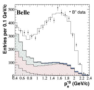
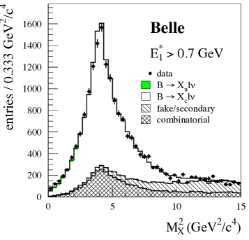
Figure 7: Belle measurements of the electron energy (left) and hadronic mass (right) spectra Urquijo:2006wd ; Schwanda:2006nf .

BaBar has measured the lepton energy and hadronic mass moments in $B\to X_{c}\ell\nu$ Aubert:2004td ; Aubert:2009qda . Furthermore, first measurements of combined hadronic mass and energy moments of the form $\langle n^{k}_{X}\rangle$ with $k=2,4,6$ are presented. They are defined as $n^{2}_{X}=M^{2}_{X}-2\widetilde{\Lambda}E_{X}+\widetilde{\Lambda}^{2}$, where $M_{X}$ and $E_{X}$ are the mass and the energy of the $X$ system and the constant $\widetilde{\Lambda}$ is taken to be 0.65 GeV. The most recent analysis is the one of hadronic mass $M(X_{c})$ moments, which are determined using a data sample of 232 million $\Upsilon(4S)\to B\bar{B}$ events Aubert:2009qda . The experimental method is similar to the Belle analysis discussed previously, i.e., one $B$ meson is fully reconstructed in a hadronic mode and a charged lepton with momentum above 0.8 GeV in the $B$ meson frame identifies the semileptonic decays of the second $B$. The remaining particles in the event are combined to reconstruct the hadronic system $X$. The resolution in $M(X_{c})$ is improved by a kinematic fit to the whole event, taking into account 4-momentum conservation and constraining the missing mass to zero. To derive the true moments from the reconstructed ones, BaBar applies a set of linear corrections. These corrections depend on the charged particle multiplicity of the $X$ system, the normalized missing mass, $E_{\mathrm{miss}}-p_{\mathrm{miss}}$, and the lepton momentum. In this way, BaBar measures the moments of the hadronic mass spectrum up to $\langle M^{6}_{X}\rangle$ for minimum lepton energies ranging from 0.8 to 1.9 GeV.

5.4.2 Determination of $|V_{cb}|$ from inclusive decays

The Heavy flavor Averaging Group (HFLAV) has used the measurements discussed in the previous section to determine $|V_{cb}|$ from a fit to HQEs of inclusive observables Amhis:2016xyh . Using expressions in the so-called kinetic scheme Benson:2003kp ; Gambino:2004qm ; Gambino:2011cq ; Alberti:2013kxa ; Alberti:2014yda and a precise determination of the $c$-quark mass, $m_{c}^{\overline{\rm MS}}(3~{}{\rm GeV})=0.986\pm 0.013$ GeV Chetyrkin:2009fv , as external input, HFLAV obtains

$$|V_{cb}| = (42.19\pm 0.78)\times 10^{-3}~{},$$ (89)

$$m_{b}^{\rm kin} = 4.554\pm 0.018~{}{\rm GeV}~{},$$ (90)

$$\mu^{2}_{\pi} = 0.464\pm 0.076~{}{\rm GeV^{2}}~{}.$$ (91)

The $\chi^{2}$ of the fit is 15.6 for $43$ degrees of freedom. Using expressions in the so-called $1S$ scheme Bauer:2004ve ; Bauer:2002sh the same set of measurements results in

$$|V_{cb}| = (41.98\pm 0.45)\times 10^{-3}~{},$$ (92)

$$m_{b}^{1S} = 4.691\pm 0.037~{}{\rm GeV}~{},$$ (93)

$$\lambda_{1} = -0.362\pm 0.067~{}{\rm GeV^{2}}~{},$$ (94)

with a $\chi^{2}$ of the fit of 23.0 for $59$ degrees of freedom. This analysis uses measurements of the photon energy moments in $B\to X_{s}\gamma$ Aubert:2005cua ; Aubert:2006gg ; Limosani:2009qg ; Chen:2001fja to constrain the $b$-quark mass and does not include higher order corrections of $O(\alpha_{s}^{2})$ and $O(\alpha_{s}/m_{b}^{2})$.

As mentioned above, the semileptonic moments have been analysed also including higher order power corrections estimated using the LSSA Gambino:2016jkc . In this case a kinetic scheme fit to the experimental data that additionally includes a constraint $m_{b}^{kin}=4.550(42)$GeV from PDG (after scheme conversion) leads to a slightly more precise value,

$$|V_{cb}| = (42.00\pm 0.64)\times 10^{-3}~{}.$$ (95)

6 Heavy-to-light inclusive

6.1 Introduction and theoretical background

Inclusive semileptonic heavy to light decays can in principle be analyzed similarly to $B\to X_{c}\ell\nu$ by using a local OPE. In practice, due to the large charm background, experimental cuts are generally imposed and reduce the “inclusivity” of the theoretical prediction. In particular, the local OPE does not converge well when the invariant mass of the hadronic system is $M_{X}\lesssim M_{D}$. In such a case the decay spectra are described using a “non-local” OPE Neubert:1993ch ; Neubert:1993um ; Bigi:1993ex , where perturbative coefficients are convoluted with non-perturbative “Shape Functions” (SFs), the $B$ meson analogs of parton distribution functions. In this SF region, the perturbative coefficients themselves can be factorized into “hard” and “jet” pieces, where the former has a typical scale of $m_{b}$ and the latter has a typical scale of $\sqrt{m_{b}\Lambda_{\mbox{\scriptsize QCD}}}$. In the infinite mass limit $m_{b}\to\infty$ there is a single non-perturbative SF. Power corrections start at $1/m_{b}$ and include multiple “subleading” SFs Lee:2004ja ; Bosch:2004cb ; Beneke:2004in ; Bauer:2001mh ; Leibovich:2002ys .

One can classify the terms based on their suppression by $1/m_{b}$ and $\alpha_{s}$. The perturbative components of the leading power term are known at $O(\alpha_{s}^{2})$ Gambino:2006wk ; Bonciani:2008wf ; Asatrian:2008uk ; Beneke:2008ei ; Bell:2008ws ; Brucherseifer:2013cu . The $1/m_{b}$ power corrections include terms convoluted with the leading power SF whose perturbative parts are known at $O(\alpha_{s})$ Paz:2009ut and terms convoluted with subleading SFs whose perturbative parts are known at $O(\alpha_{s}^{0})$ Lee:2004ja ; Bosch:2004cb ; Beneke:2004in . At this order one can still use subleading functions of one light-cone variable. The inclusion of $O(\alpha_{s})$ contributions of subleading SFs requires functions of multiple light-cone momenta in analogy to higher twist effects in Deep Inelastic Scattering Ellis:1982cd . Schematically, in the SF region we have the factorization formula

$$d\Gamma\sim H\cdot J\otimes S+\frac{1}{m_{b}}\sum_{i}\,h\cdot J_{0}\otimes s_{i}+\frac{1}{m_{b}}\sum_{k}\,h\cdot j_{k}\otimes S+\,O\left(\frac{1}{m_{b}^{2}}\right)\,,$$ (96)

where $H$ is the leading power hard function, $J$ is the leading power jet function, both known at $O(\alpha_{s}^{2})$, $J_{0}$ is the $O(\alpha_{s}^{0})$ part of $J$, $h=1+O(\alpha_{s})$, $s_{i}$ are given in Refs. Lee:2004ja ; Bosch:2004cb ; Beneke:2004in , and $j_{k}$ in Ref. Paz:2009ut . The symbol $\otimes$ denotes an integral over the light-cone momentum.

The moments of the leading and subleading SFs are related to the HQE parameters measured in the inclusive semileptonic decays to charm. The relations are known for the leading SF up to at least the fifth moment Gunawardana:2017zix , although the current large uncertainty of higher HQE parameters Mannel:2010wj ; Gambino:2016jkc might limit the use of higher moments relations. The formalism in Ref. Gunawardana:2017zix allows to construct such relations for the subleading SFs too, but at present only the first three moments are known Bauer:2001mh ; Bauer:2002yu . A detailed knowledge of the SFs is necessary only in a portion of the phase space where $p_{+}=E_{X}-p_{X}\sim\Lambda_{\rm QCD}$; elsewhere only the first few moments of the SFs are relevant and one recovers the local OPE description.

The present $|V_{ub}|$ determination by HFLAV Amhis:2016xyh is based on various approaches which are all rooted in (96) and differ in the inclusion and treatment of perturbative and nonperturbative contributions, see Ref. Antonelli:2009ws for a detailed discussion.

The approach known as BLNP (Bosch-Lange-Neubert-Paz) Lange:2005yw aimed at a precision extraction of $|V_{ub}|$ from $B\to X_{u}\ell\nu$ and $B\to X_{s}\gamma$, based on the knowledge in 2005. It used the first two terms in (96), in particular the $O(\alpha_{s})$ expression for $H\cdot J\otimes S$ and the $O(\alpha^{0}_{s})$ expression for the $h\cdot J_{0}\otimes s_{i}$ terms. Kinematical corrections that scale as $\alpha_{s}/m_{b}$ and $\alpha_{s}/m^{2}_{b}$ DeFazio:1999ptt , as well as $1/m_{b}^{2}$ corrections Manohar:1993qn ; Blok:1993va , for which factorization formulas were not known, were also included by convolution with the leading power shape function. Using Renormalisation Group methods $H$ is evolved from “hard” to the “jet” scale to resum Sudakov double logs. As for the non-perturbative inputs, the leading order SF was to be taken from $B\to X_{s}\gamma$ and subleading SFs $s_{i}$ to be modeled using $\sim 700$ models. In practice, the current treatment of $S$ by experiments is to use an exponential or Gaussian model constrained by the first two moments of $S$ obtained from the global fit of HQE parameters in the kinetic scheme Amhis:2016xyh .

Since Ref. Lange:2005yw appeared, there have been many theoretical advances. Two-loop calculations of $H$ Bonciani:2008wf ; Asatrian:2008uk ; Beneke:2008ei ; Bell:2008ws and $J$ Becher:2006qw as well as one-loop calculation of $j_{k}$ Paz:2009ut became available. The free quark differential decay rate were calculated at $O(\alpha_{s}^{2}\beta_{0})$ Luke:1994du ; Bauer:2001rc ; Hoang:2005pj ; Gambino:2006wk and at complete $O(\alpha_{s}^{2})$ Brucherseifer:2013cu . Running effects from the “hard” to the “jet” at $O(\alpha_{s}^{2})$ were studied Greub:2009sv . It was found there that the factorization of the perturbative coefficient into jet and hard functions is not strictly necessary. More recently, three loop calculations of $J$ Bruser:2018rad and the partonic $S$ Bruser:2019yjk were performed. Implementing these within the BLNP framework would probably require also the calculation of $H$ at three-loops, which is not available yet. There were also theoretical advances in the description of non-perturbative effects in $B\to X_{s}\gamma$ Lee:2006wn ; Benzke:2010js ; Benzke:2010tq . In particular, new subleading shape functions unique to $B\to X_{s}\gamma$ were identified Benzke:2010js , making it more difficult to use data from radiative $B$ decays as input for the extraction of $|V_{ub}|$. These new features are not yet implemented in the BLNP approach. An alternative implementation of the same conceptual framework has been presented in Ref. Ligeti:2008ac , together with a systematic procedure to account for the uncertainties in the modelling of the leading SF, to be discussed below.

The GGOU (Gambino-Giordano-Ossola-Uraltsev) approach Gambino:2007rp avoids the expansion in $1/m_{b}$ and the introduction of subleading SFs. The perturbative coefficients are computed at fixed order to $O(\alpha_{s}^{2}\beta_{0})$ in the kinetic scheme. The effect of RGE evolution in the SF region and all subleading SFs are absorbed into three $q^{2}$-dependent SF $F_{i}(k,q^{2})$, whose first moments are fixed by present semileptonic fits. The uncertainty due to the functional form is estimated comparing $\sim 100$ models.

The emergence of the SF can also be seen in perturbation theory: soft-gluon resummation together with an infrared prescription gives rise to a $b$ quark SF. In the DGE (Dressed-Gluon Exponentiation) approach Andersen:2005mj ; Gardi:2008bb this is achieved by an internal resummation of running coupling corrections in the Sudakov exponent, thus providing a perturbative model for the leading SF. A somewhat similar line of action is followed in Ref. Aglietti:2007ik where the infrared prescription is provided by the so-called analytic QCD coupling.

The so-called Weak Annihilation (WA) contributions are a source of theoretical uncertainty common to all approaches. In the local OPE they emerge at $O(1/m_{b}^{3})$ but are enhanced by a large Wilson coefficient Bigi:1993bh and may give rise to a difference between $B^{+}$ and $B^{0}$ decays. As they are expected to be much more important in charm decays, the latter constrain them most effectively at present. In particular, the $D^{0}$, $D^{+}$ and $D_{s}$ total semileptonic rates and the electron spectra measured by the CLEO Collaboration Asner:2009pu have been employed Bigi:2009ym ; Ligeti:2010vd ; Gambino:2010jz . From the absence of clear indications for WA effects in semileptonic charm decays, one can conclude that the WA correction to the total rate of $B\to X_{u}\ell\nu$ must be smaller than about 2% Gambino:2010jz . However, WA is localized in the high $q^{2}$ region and therefore the related uncertainty on $|V_{ub}|$ depends on the kinematical cuts, and this is taken into account in the current HFLAV averages. Because the high $q^{2}$ tail is particularly sensitive to higher power corrections (and not to the SFs), see for instance Refs. Bauer:2000xf ; Bauer:2001rc ; Gambino:2007rp , one might eventually expect the cleanest determinations of $|V_{ub}|$ to come from the low $q^{2}$ region only. An upper cut on $q^{2}$ might therefore be beneficial Lange:2005yw ; Gambino:2007rp .

A few recent experimental analyses Urquijo:2009tp ; Lees:2011fv have relaxed the kinematic cuts, making use of experimental information to subtract the background. As a result, most of the $B\to X_{u}\ell\nu$ phase space is taken into account and the sensitivity to the SFs is substantially reduced, while a description based on the local OPE sets in. In these cases the quoted theoretical uncertainties are smaller, but one should keep in mind that these analyses still depend on the SFs treatment and modelling for the determination of the reconstruction efficiencies, whose uncertainty contribute to the final experimental systematic error. As will be discussed later on, a realistic signal simulation requires the implementation of so-called hybrid models that transform the inclusive predictions of the approaches mentioned above into individual final hadronic states. The uncertainties related to such hybrid models remain a major issue for the inclusive determination of $|V_{ub}|$.

6.2 Status of the experimental results

The most difficult task of the inclusive measurements is the discrimination between the $B\to X_{u}\ell\nu$ signal and the much more abundant decays involving Cabibbo-favoured $B\to X_{c}\ell\nu$ decays. The signal events are studied in restricted regions of the phase space to improve the signal-to-background ratio. Compared to $B\to X_{c}\ell\nu$ events, the signal tends to have higher lepton momenta $p_{\ell}$, lower invariant mass of the $X_{u}$ state $M_{X}$, higher $q^{2}$, and smaller values of the light-cone momentum $P_{+}=E_{X}-|\bm{p}_{X}|$, where $E_{X}$ and $\bm{p}_{X}$ are energy and momentum of the hadronic system $X_{u}$ in the $B$ meson rest frame. As explained above, these restrictions introduce difficulties in the calculation of the expected partial branching fraction, enhancing perturbative and nonperturbative QCD corrections which lead to large theoretical uncertainties in the measurement of $|V_{ub}|$.

The measurement of the partial branching fraction $\Delta\cal{B}$ can be obtained with tagged or untagged analyses.

6.2.1 Tagged Analyses

In tagged analyses, the $\Upsilon(4S)\to B{\overline{B}}$ events are identified by reconstructing one of the $B$ mesons, $B_{reco}$, via fully hadronic decays. The signal decay of the second $B$ meson ($B_{signal}$) is identified just by the presence of an electron or a muon. The tracks and neutral objects not associated with the $B_{reco}$ can be uniquely assigned to the signal side, so that the inclusive $X_{u}$ state can be clearly reconstructed. The neutrino four-momentum $p_{\nu}$ can be estimated from the missing momentum $p_{miss}=p_{e^{+}e^{-}}-p_{B_{reco}}-p_{X_{u}}-p_{\ell}$, where $p_{e^{+}e^{-}}$ is the initial state four-momentum. From this, all the kinematic variables of the signal state can be easily computed.

Because the momentum of the signal $B$ meson is determined from of the $B_{reco}$, the signal decay products can be computed directly in the $B$-meson rest frame, resulting in an improved resolution of the accessible observables. Moreover, the constrained kinematics allow for a better separation of the signal from the background.

The downside of the tagged analysis is the low signal efficiency (about 0.3-0.5%) which implies that for kinematic variables like the lepton momentum $p_{\ell}$, the untagged analyses at the B-factories can give competitive or better results. Undetected and poorly reconstructed tracks or photons lead to irreducible background from the dominant $B\to X_{c}$ decays even in regions of the phase space potentially free of such background, and this can affect the final resolution on the signal kinematics.

The hadronic $B$-tagging approach was used for the first time by BaBar to extract the $B\to X_{u}\ell\nu$ signal in the phase space region $M_{X}<1.55$ GeV, with the further requirement that $p_{\ell}>1$ GeV Aubert:2003zw . Using the same sample, BaBar removed the constraint on $M_{X}$ and obtained the $B\to Xu\ell\nu$ partial branching ratio requiring only $P_{\ell}>1$ GeV, which covers about $90\%$ of the signal phase space Aubert:2006qi . This challenging analysis was affected by the large statistical uncertainties and limited by the knowledge on the $B\to X_{c}$ background components and the signal composition available when it was published.

Exploiting the full datasets collected, both Belle  Urquijo:2009tp and BaBar  Lees:2011fv published measurements of $B\to X_{u}\ell\nu$ partial branching fraction, performing a fit in $M_{X}$ and $q^{2}$, and requiring only $p_{\ell}>1$ GeV. BaBar determined also the partial branching fractions in other several restricted regions of the phase space.

6.2.2 Untagged Analyses

The untagged measurements allow to collect large samples but are affected by considerable backgrounds. The untagged measurements have access only to a few kinematic variables, namely the lepton momentum $p_{\ell}$, and the $q^{2}$ spectra,

• lepton spectrum: this can be studied inclusively without requirements on the rest of the event. In this case the momentum spectrum can only be given in the $\Upsilon(4S)$ rest frame.

• $q^{2}$ distribution: this requires the reconstruction of the neutrino 4-momentum, which exploits the high hermeticity of the $B$ factories’ detectors. The neutrino 4-momentum is given by the event missing 4-momentum, $p_{miss}=p_{e^{+}e^{-}}-p_{vis}$, where $p_{e^{+}e^{-}}$ is the initial state 4-momentum, and $p_{vis}$ is the total visible 4-momentum determined by all the charged tracks from the collision point, identified pairs of charged tracks from $K_{s}$, $\Lambda$ and $\gamma\to e^{+}e^{-}$, and energy deposits in the electromagnetic calorimeter.

The lepton momentum spectrum is affected by large backgrounds from $B\to X_{c}\ell\nu_{\ell}$ via the $D\ell\nu$, $D^{*}\ell\nu$, $D^{**}\ell\nu$ (where by $D^{**}$ is a mixture of charm excited state and non resonant $D^{(*)}-n\pi$ transitions), $D_{s}K\ell\nu X$ and also secondary leptons from $D$ mesons decays, and a background from $e^{+}e^{-}\to q\overline{q}$ events, where the main contribution comes from $c\overline{c}$, which is assessed from control data samples recorded below the $\Upsilon(4S)$ resonance. Because of the large background, usually the signal is extracted only for regions with high momentum lepton, typically $p_{\ell}>1.9-2.1$ GeV. Old analyses of the lepton endpoints are from CLEO Bornheim:2002du , Belle Limosani:2005pi and BaBar Aubert:2005mg .

Recently, BaBar published a study TheBABAR:2016lja of the lepton spectrum using the full data set, and exploiting all the knowledge about the rate and the form factors of the various $B\to X_{c}\ell\nu$ exclusive decays which are the major source of backgrounds. The signal is extracted from a fit to the electron momentum spectrum, which is described as the sum of predicted signal (model dependent shape) and various specific backgrounds yields with shapes fixed by MC. The fit covers lepton momentum in the $\Upsilon(4S)$ rest frame from 0.8 to 2.7 GeV, in 50 MeV bins, except for the data in the interval 2.1 to 2.7 GeV which are combined in a single bin to avoid effects from differences in the shape of the theoretically predicted signal spectrum. In a given momentum interval, the excess of events above the sum of the fitted background contributions is taken as the number of signal events.

An important difference of this analysis with respect to the other ones is that different theoretical models are considered in the extraction of the partial branching fractions. Instead, all other measurements determine the partial branching fraction by using a single model, and its partial rate is then converted in a measurement of $|V_{ub}|$ by taking the corresponding partial rate predicted by the theory calculations.

The extracted inclusive signal branching fractions and the values of $|V_{ub}|$ agree well for GGOU and DGE, although they are about 13% smaller than the average of the other measurements. This difference can be attributed to the shape of the predicted signal spectrum and/or the shapes of some of the large background contributions above 2 GeV where the signal fraction is largest. On the other hand, the value of $|V_{ub}|$ based on BLNP agrees well with other measurements.

A subset of all the measurements of the inclusive $|V_{ub}|$ are reported in Fig.8 for the various frameworks considered, see Amhis:2019ckw for more details.

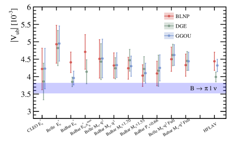
Figure 8: Measurements of inclusive $|V_{ub}|$ and their averages based on BLNP, DGE and GGOU calculations. The HFLAV average of $|V_{ub}|$ results from $B\to\pi\ell\nu_{\ell}$ decay is also reported for comparison.

6.2.3 Lessons learned from the past

The measurements based on tagged samples have considerably larger statistical uncertainties. The sample size allows for only a few bins in the 2D fit, but there are regions of the phase space (e.g. low $M_{X}$) where the background fractions are modest. The current sensitivity to the details of the shapes of the signal and background distributions is however limited.

For untagged measurements only the high end of the spectrum is sensitive to the signal and also to the background near their kinematic endpoints. Both approaches have their pros and cons, given the size of the currently available data. The latest BaBar measurement of the lepton spectrum, shows a high dependence of the result from the signal model. The same effect, even if not directly evident, was observed also in tagged measurements from the sensitivity of the signal yield extraction on the shape function parameters in the analyses that cover larger portion of the phase space.

Semileptonic $B\to X_{u}\ell\nu$ decays are simulated as a combination of resonant decays with $X_{u}=\pi,\eta,\eta^{\prime},\rho,\omega$, and decays to nonresonant hadronic final states $X_{u}$. The latter is simulated with a continuous invariant mass spectrum following the theory predictions by De Fazio and Neubert DeFazio:1999ptt , which depend on the SF parameters and $m_{b}$. The nonresonant and the resonat part are combined such that the sum of their branching fractions is equal to the measured one for the inclusive $B\to X_{u}\ell\nu$. The events generated with this model, are reweighted to obtain predictions for different SF parameters and different branching fraction of the resonant states. This model is usually called ”hybrid model”. Belle in Urquijo:2009tp , corrects the hybrid model to match the moments of the $M_{X}$ and $q^{2}$ distributions predicted by the the GGOU model. A picture of the model of the invariant mass $M_{X}$ shape used to describe the $B\to X_{u}\ell\nu$ is reported in Fig.9.

Figure 9: Model of the hadronic invariant mass $M_{X}$ for the signal $B\to X_{u}\ell\nu$ events, separately for $B^{0}$ (top) and $B^{+}$ (bottom).

Another effect not considered so far, is the impact of the fragmentation of the generated $u$ quark into final state hadrons, which is performed using JETSET. The modeling of the final state multiplicity could affect both the signal efficiency and the signal templates used to separate signal from background.

The measurement of the partial branching fraction separately for neutral and changed $B$ mesons has been used to constrain the WA contribution. Both tagged approach, in various regions of the phase space Lees:2011fv , and untagged approach, in the high lepton region Aubert:2007tw , have been used, but these have given weak upper limits mainly because of the large statistical uncertainties. More stringent upper limit on WA has been obtained by CLEO which used a model dependent approach studying the high $q^{2}$ region in $B\to X_{u}\ell\nu$ decays Rosner:2006zz . Both these bounds are milder than those estimated from $D$ and $D_{s}$ semileptonic decays in Refs.Ligeti:2010vd ; Gambino:2010jz which were mentioned above.

In the tagged measurements the suppression of the $b\to c$ background is performed by vetoing events where a $K^{+}$ or a $K_{s}^{0}$ is detected in the hadronic $X$ system. This causes a loss in the signal contribution where a $s{\bar{s}}$ pair is produced (usually called $s{\bar{s}}$-popping). The fraction of these events is about $12\%$ of the non-resonant component and it is fixed in the fragmentation parameters of JETSET/PYTHIA. The uncertainty on this fraction is assumed to be about $30\%$, so for analyses that aim to cover larger regions of the phase space, with higher statistics this could be an irreducible source of systematic uncertainty. This is another point that should be improved in future analyses at Belle II.

6.3 Fitting distributions: SIMBA and NNVub

As we discussed above, SFs modelling is an important source of theoretical uncertainty in the study of $B\to X_{u}\ell\nu$ and particularly in the extraction of $|V_{ub}|$ from these decays. While the first few moments of the SFs must satisfy OPE constraints, direct experimental information on the SFs is somewhat limited. Indeed, the measured photon spectrum in $B\to X_{s}\gamma$ is sensitive to a different set of subleading SFs. However differential distributions in $B\to X_{u}\ell\nu$ such as the lepton energy and the invariant mass distributions depend directly on all the SFs and can therefore be used to constrain them. Conversely, they can be used to validate SFs models and approaches where the SFs are calculated, such as DGE. The high luminosity expected makes the measurement of differential distributions possible at Belle II.

The extraction of $|V_{ub}|$ performed by HFLAV in the BLNP and GGOU frameworks assumes a set of two-parameter functional forms, and it is unclear to what extent the chosen set is representative of the available functional space, and whether the estimated uncertainty really reflects the limited knowledge of the SFs. This point was first emphasized in Ref. Ligeti:2008ac , where a different strategy was proposed, based on the expansion of the leading SF in a basis of orthogonal functions, whose coefficients are fitted to the $B\to X_{s}\gamma$ spectrum, and on the modeling of the subleading SFs. The SIMBA project Bernlochner:2013gla aims at performing a global fit to $B\to X_{s}\gamma$ and $B\to X_{u}\ell\nu$ spectra, to simultaneously determine $|V_{ub}|$, $m_{b}$, the leading SF, as well as the Wilson coefficient of radiative $b$ decays. Additional external constraints, such from $B\to X_{c}\ell\nu$, can also be employed.

Another strategy, called NNVub and explored in Gambino:2016fdy for the GGOU approach, employs artificial neural networks as unbiased interpolants for the SFs, in a way similar to what the NNPDF Collaboration do in fitting for Parton Distribution Functions Ball:2008by . This method allows for unbiased estimates of the SFs functional form uncertainty, and for a straightforward implementation of new experimental data, including $B\to X_{s}\gamma$ and $B\to X_{u}\ell\nu$ spectra and other inputs on quark masses and OPE matrix elements. Both SIMBA and NNVub appear well posed to analyse the Belle II data in a model independent and efficient way.

6.4 Prospect for the future: Belle II outlook

The measurements of fully differential spectra on the kinematic variables, e.g. $q^{2}$, $M^{2}_{X}$, $p^{\pm}_{X}$, $E_{l}$, and separate measurements for charged and neutral B-meson decays are required to allow for an improved extraction of $|V_{ub}|$ in the long term. Therefore, the future measurements should provide these unfolded spectra independent of theoretical assumptions.

Combining both $B\to X_{u}\ell\nu$ and $B\to X_{s}\gamma$ as well as constraints on the SF moments from $B\to X_{c}\ell\nu$ in a global fit can simultaneously provide the inclusive $|V_{ub}|$ and the leading SF functional form with its uncertainties as they follow from the uncertainties in the included experimental measurements. Fig. 10 shows the projections for a global fit in the SIMBA framework with two projected single-differential spectra of $M_{X}$ and $E_{\ell}$ for $B\to X_{u}\ell\nu$ and a $E_{\gamma}$ spectrum for $B\to X_{s}\gamma$ from 1 ab^-1 and 5 ab^-1 Belle II data set Kou:2018nap .

Figure 10: Belle II projection for a global fit in the SIMBA approach of $|V_{ub}|$ with 1 ab^-1 and 5 ab^-1. Theory uncertainties are not included in the fit and are expected to be of similar size.

The new tagging algorithm developed for Belle II can perform better than the old neural network method used in the previous Belle publications with about 3 times higher efficiency Keck:2018lcd . With a larger data set, the systematic uncertainties counted for reconstruction efficiencies, fake leptons and continuum background knowledge are expected to improve for this measurement. The projections for inclusive $|V_{ub}|$ are summarized in Table 6.

Table 6: Expected percentage uncertainties in inclusive $|V_{ub}|$ measurements with the Belle full data sample, 5 ab^-1 and 50 ab^-1 Belle II data Kou:2018nap .

Int. Luminosity	Statistical	Systematic (reducible, irreducible)	Total Exp.	Theory	Total
605 fb-1 (old B tag)	4.5	(3.7, 1.6)	6.0	2.5-4.5	6.5-7.5
5 ab-1	1.1	(1.3, 1.6)	2.3	2.5-4.5	3.4-5.1
50 ab-1	0.4	(0.4, 1.6)	1.7	2.5-4.5	3.0-4.8

7 Outlook

We have summarized our main results in Sec. 1. In this final Section, we would like to look at the prospects of our field over the next five years. What can we expect for semileptonic $b$ decays at the two main experiments? What kind of progress can we reasonably anticipate in lattice QCD and continuum calculations?

Belle II has started data taking with a complete detector in March 2019 and recorded about 10/fb in its first year of operation. By introducing the crab waist scheme at the collision point, SuperKEKB achieved the world’s highest instantaneous luminosity of $2.4\times 10^{34}/$cm²/s in June 2020 with acceptable background conditions for Belle II to take data. In total 64/fb of $\Upsilon(4S)$ data were recorded in the spring 2020 run, bringing the total to 74/fb. Data taking will resume in October 2020 with the goal to reach a total integrated luminosity of more than 100/fb before the end of the year break. Belle II plans to accumulate a data set equivalent to the Belle luminosity of about 1/ab by the end of 2021. In 2022 the experiment will enter a long shutdown to install the second pixel detector layer and replace the silicon photomultipliers in the barrel particle identification device. Data taking will resume in 2023 and by 2025 Belle II expects to have recorded a data sample exceeding 10/ab.

Given these luminosity prospects, competitive Belle II results for semileptonic $B$ decays can be expected in the years to follow. In addition, a three times more efficient hadronic tag and better low momentum tracking of the slow pion from the $D^{*}$ decay will further benefit semileptonic analyses in particular. This will allow to take a fresh look at the CKM matrix element magnitudes $|V_{cb}|$ and $|V_{ub}|$ and to improve measurements which are still statistically limited, such as $R(D)$ and $R(D^{*})$.

The LHCb experiment has shown great capabilities with the results on $R(D^{*})$, $|V_{ub}|/|V_{cb}|$ with $\Lambda_{b}$ decays, and $|V_{cb}|$ with $B_{s}$ decays. These measurements are based on the data collected in 2011 and 2012 (Run 1), corresponding at $3/$fb of integrated luminosity. The data collected in 2015-2018 (Run 2) at $pp$ collision energy of $\sqrt{s}=13~{}$ TeV, correspond to about $6/$fb of integrated luminosity. There are various ongoing analyses on the full dataset. Most of the measurements are limited by systematic uncertainties, among which the largest ones are generally due to external inputs from other experiments and to the limited available samples of Monte Carlo simulations. Nevertheless the large dataset available is going to be fully exploited.

The LHCb experiment is at present undergoing a major upgrade of the detector. The construction and commissioning should end in 2021, when LHC will resume the activity. The upgrade will allow to collect data at higher instantaneous luminosity, so about five $pp$ collisions per bunch crossing are foreseen, to be compared with about one-two $pp$ collisions in Run1 and Run2. To handle the higher occupancy expected in the detector, besides the improvements in the various subdetectors, a full software L0 trigger will be employed. The software L0 trigger will add flexibility to the data taking, allowing to reduce the thresholds for muon and hadron trigger decisions, enlarging in this way the physics capabilities. The analyses of semileptonic decays with taus and electrons will benefit from the lower trigger thresholds in terms of signal efficiencies. With this upgraded detector, LHCb is planning to integrate a luminosity of $23/$fb by 2024, and to collect a total sample of $50/$fb by 2028-2029, after LHC will have switched to higher luminosity.

By now, lattice QCD is the tool of choice for the form factors describing semileptonic decays of $b$-hadrons. At present, the most urgent need is the $q^{2}$ (or, equivalently, $w$) dependence of the form factors of $B\to D^{*}l\nu$, both to see how the form-factor slopes affect the $|V_{cb}|$ determination and to solidify the SM prediction of $R(D^{*})$. A few such calculations are underway. Given the success of LHCb with $\Lambda_{b}$ semileptonic decays, updates of the baryon form factors are desirable, and we encourage other lattice-QCD practitioners to turn their attention to these decays. Another topic for future research are rigorous calculations with a $\rho$ or $\phi$ vector meson in the final state.

The leptonic decay constants are now at the subpercent level of uncertainty, and the prospects for extending these methods to semileptonic form factors are underway. In general, near-term lattice-QCD calculations of this precision will be based on the MILC collaboration’s HISQ ensembles, which, among all lattice data sets, span the largest range of lattice spacing at physical light-quark masses and with high statistics. We consider it important that other ensemble sets be extended to a similar range, to enable further (sub)percent-level calculations with different systematics from the fermion discretization.

The inclusive determination of $|V_{cb}|$ will benefit from the calculation of new higher order effects, such as the $O(\alpha_{s}^{3})$ contributions to the total width, and from a reassessment of QED effects. However, the next frontier is represented by the integration with lattice QCD calculations to improve the determination of HQE matrix elements, and eventually by the calculation of the inclusive rates directly on the lattice. For what concerns inclusive charmless decays, the general theoretical framework appears solid but needs to be updated in the light of recent higher order calculations and should be extensively validated by experimental data which will become available at Belle II. In particular, the measurement of the lepton energy and hadronic invariant mass distributions will provide important information on the Shape Functions, while the $q^{2}$ distribution will allow us to constrain and possibly avoid the effect of Weak Annihilation. The wealth of data expected at Belle II, a close cooperation between theorists and experimentalists, and hopefully new lattice data should help resolve various open issues, so that we might eventually expect the uncertainty on inclusive $|V_{ub}|$ to become lower than 3%.

- (1) N. Cabibbo, Phys. Rev. Lett. 10, 531 (1963). DOI 10.1103/PhysRevLett.10.531
- (2) M. Kobayashi, T. Maskawa, Prog. Theor. Phys. 49, 652 (1973). DOI 10.1143/PTP.49.652
- (3) S. Aoki, et al., arXiv:1902.08191 [hep-lat] (2019)
- (4) R. Aaij, et al., Eur. Phys. J. C79(8), 675 (2019). DOI 10.1140/epjc/s10052-019-7112-x
- (5) C.G. Boyd, B. Grinstein, R.F. Lebed, Phys. Lett. B353, 306 (1995). DOI 10.1016/0370-2693(95)00480-9
- (6) C.G. Boyd, B. Grinstein, R.F. Lebed, Phys. Rev. D56, 6895 (1997). DOI 10.1103/PhysRevD.56.6895
- (7) I. Caprini, B. Grinstein, R.F. Lebed, Phys. Rev. D96(3), 036015 (2017). DOI 10.1103/PhysRevD.96.036015
- (8) C. Bourrely, I. Caprini, L. Lellouch, Phys.Rev. D79, 013008 (2009). DOI 10.1103/PhysRevD.82.099902, 10.1103/PhysRevD.79.013008
- (9) G.P. Lepage, S.J. Brodsky, Phys. Rev. D22, 2157 (1980). DOI 10.1103/PhysRevD.22.2157
- (10) R. Akhoury, G.F. Sterman, Y.P. Yao, Phys. Rev. D50, 358 (1994). DOI 10.1103/PhysRevD.50.358
- (11) I. Caprini, L. Lellouch, M. Neubert, Nucl. Phys. B530, 153 (1998). DOI 10.1016/S0550-3213(98)00350-2
- (12) D. Bigi, P. Gambino, S. Schacht, JHEP 11, 061 (2017). DOI 10.1007/JHEP11(2017)061
- (13) M. Neubert, Z. Ligeti, Y. Nir, Phys. Lett. B301, 101 (1993). DOI 10.1016/0370-2693(93)90728-Z
- (14) M. Neubert, Z. Ligeti, Y. Nir, Phys. Rev. D47, 5060 (1993). DOI 10.1103/PhysRevD.47.5060
- (15) Z. Ligeti, Y. Nir, M. Neubert, Phys. Rev. D49, 1302 (1994). DOI 10.1103/PhysRevD.49.1302
- (16) W. Detmold, C. Lehner, S. Meinel, Phys. Rev. D92(3), 034503 (2015). DOI 10.1103/PhysRevD.92.034503
- (17) E. Follana, Q. Mason, C. Davies, K. Hornbostel, G. Lepage, J. Shigemitsu, H. Trottier, K. Wong, Phys. Rev. D 75, 054502 (2007). DOI 10.1103/PhysRevD.75.054502
- (18) A.X. El-Khadra, A.S. Kronfeld, P.B. Mackenzie, Phys. Rev. D 55, 3933 (1997). DOI 10.1103/PhysRevD.55.3933
- (19) M.B. Oktay, A.S. Kronfeld, Phys. Rev. D 78, 014504 (2008). DOI 10.1103/PhysRevD.78.014504
- (20) C.T.H. Davies, C. McNeile, E. Follana, G.P. Lepage, H. Na, J. Shigemitsu, Phys. Rev. D82, 114504 (2010). DOI 10.1103/PhysRevD.82.114504
- (21) J. Harada, S. Hashimoto, A.S. Kronfeld, T. Onogi, Phys. Rev. D 65, 094514 (2002). DOI 10.1103/PhysRevD.65.094514
- (22) C. McNeile, C. Davies, E. Follana, K. Hornbostel, G. Lepage, Phys. Rev. D 86, 074503 (2012). DOI 10.1103/PhysRevD.86.074503
- (23) A. Bazavov, et al., Phys. Rev. D98(7), 074512 (2018). DOI 10.1103/PhysRevD.98.074512
- (24) E. McLean, C.T.H. Davies, A.T. Lytle, J. Koponen, Phys. Rev. D99(11), 114512 (2019). DOI 10.1103/PhysRevD.99.114512
- (25) T. Kaneko, Y. Aoki, G. Bailas, B. Colquhoun, H. Fukaya, S. Hashimoto, J. Koponen, in 37th International Symposium on Lattice Field Theory (2019)
- (26) B. Blossier, et al., JHEP 04, 049 (2010). DOI 10.1007/JHEP04(2010)049
- (27) A. Bussone, et al., Phys. Rev. D93(11), 114505 (2016). DOI 10.1103/PhysRevD.93.114505
- (28) M. Okamoto, et al., Nucl. Phys. B Proc. Suppl. 140, 461 (2005). DOI 10.1016/j.nuclphysbps.2004.11.151
- (29) S.W. Qiu, C. DeTar, A.X. El-Khadra, A.S. Kronfeld, J. Laiho, R.S. Van de Water, PoS LATTICE2013, 385 (2014). DOI 10.22323/1.187.0385
- (30) M. Atoui, V. Morénas, D. Beˇcirevic, F. Sanfilippo, Eur. Phys. J. C 74(5), 2861 (2014). DOI 10.1140/epjc/s10052-014-2861-z
- (31) J.A. Bailey, et al., Phys. Rev. D92(3), 034506 (2015). DOI 10.1103/PhysRevD.92.034506
- (32) H. Na, C.M. Bouchard, G.P. Lepage, C. Monahan, J. Shigemitsu, Phys. Rev. D92(5), 054510 (2015). DOI 10.1103/PhysRevD.93.119906, 10.1103/PhysRevD.92.054510. [Erratum: Phys. Rev.D93,no.11,119906(2016)]
- (33) C.J. Monahan, H. Na, C.M. Bouchard, G.P. Lepage, J. Shigemitsu, Phys. Rev. D 95(11), 114506 (2017). DOI 10.1103/PhysRevD.95.114506
- (34) E. McLean, C. Davies, J. Koponen, A. Lytle, Phys. Rev. D 101(7), 074513 (2020). DOI 10.1103/PhysRevD.101.074513
- (35) A. Kobach, Physics Letters B 809, 135708 (2020). DOI 10.1016/j.physletb.2020.135708. URL http://dx.doi.org/10.1016/j.physletb.2020.135708
- (36) M. Bordone, N. Gubernari, M. Jung, D. van Dyk, Eur. Phys. J. C 80(4), 347 (2020). DOI 10.1140/epjc/s10052-020-7850-9
- (37) J.A. Bailey, et al., Phys. Rev. D89(11), 114504 (2014). DOI 10.1103/PhysRevD.89.114504
- (38) C. Monahan, J. Shigemitsu, R. Horgan, Phys. Rev. D 87(3), 034017 (2013). DOI 10.1103/PhysRevD.87.034017
- (39) J. Harrison, C. Davies, M. Wingate, Phys. Rev. D97(5), 054502 (2018). DOI 10.1103/PhysRevD.97.054502
- (40) A. Vaquero, C. DeTar, A. El-Khadra, A. Kronfeld, J. Laiho, R. Van de Water, in 17th Conference on Flavor Physics and CP Violation (2019)
- (41) T. Bhattacharya, B.J. Choi, R. Gupta, Y.C. Jang, S. Jwa, S. Lee, W. Lee, J. Leem, S. Park, PoS LATTICE2019, 056 (2019)
- (42) E. McLean, C. Davies, A. Lytle, J. Koponen, PoS LATTICE2018, 281 (2019). DOI 10.22323/1.334.0281
- (43) A. Lytle, B. Colquhoun, C. Davies, J. Koponen, C. McNeile, PoS BEAUTY2016, 069 (2016). DOI 10.22323/1.273.0069
- (44) B. Colquhoun, C. Davies, J. Koponen, A. Lytle, C. McNeile, PoS LATTICE2016, 281 (2016). DOI 10.22323/1.256.0281
- (45) J. Flynn, R. Hill, A. Jüttner, A. Soni, J.T. Tsang, O. Witzel, in 37th International Symposium on Lattice Field Theory (2019)
- (46) A. Datta, S. Kamali, S. Meinel, A. Rashed, JHEP 08, 131 (2017). DOI 10.1007/JHEP08(2017)131
- (47) R. Aaij, et al., Phys. Rev. D96(11), 112005 (2017). DOI 10.1103/PhysRevD.96.112005
- (48) P. Böer, M. Bordone, E. Graverini, P. Owen, M. Rotondo, D. Van Dyk, JHEP 06, 155 (2018). DOI 10.1007/JHEP06(2018)155
- (49) Y.S. Amhis, et al., arXiv:1909.12524 (2019)
- (50) R. Glattauer, et al., Phys. Rev. D93(3), 032006 (2016). DOI 10.1103/PhysRevD.93.032006
- (51) E. Waheed, et al., Phys. Rev. D100(5), 052007 (2019). DOI 10.1103/PhysRevD.100.052007
- (52) W. Dungel, et al., Phys. Rev. D82, 112007 (2010). DOI 10.1103/PhysRevD.82.112007
- (53) A. Abdesselam, et al., arXiv:1702.01521 [hep-ex] (2017)
- (54) D. Bigi, P. Gambino, S. Schacht, Phys. Lett. B769, 441 (2017). DOI 10.1016/j.physletb.2017.04.022
- (55) B. Grinstein, A. Kobach, Phys. Lett. B771, 359 (2017). DOI 10.1016/j.physletb.2017.05.078
- (56) J.P. Lees, et al., Phys. Rev. Lett. 123(9), 091801 (2019). DOI 10.1103/PhysRevLett.123.091801
- (57) R. Aaij, et al., arXiv:2001.03225 (2020)
- (58) J.P. Lees, et al., Phys. Rev. Lett. 109, 101802 (2012). DOI 10.1103/PhysRevLett.109.101802
- (59) J.P. Lees, et al., Phys. Rev. D88(7), 072012 (2013). DOI 10.1103/PhysRevD.88.072012
- (60) M. Huschle, et al., Phys. Rev. D92(7), 072014 (2015). DOI 10.1103/PhysRevD.92.072014
- (61) A. Abdesselam, et al., arXiv:1904.08794 (2019)
- (62) S. Hirose, et al., Phys. Rev. Lett. 118(21), 211801 (2017). DOI 10.1103/PhysRevLett.118.211801
- (63) S. Hirose, et al., Phys. Rev. D97(1), 012004 (2018). DOI 10.1103/PhysRevD.97.012004
- (64) R. Aaij, et al., Phys. Rev. Lett. 115(11), 111803 (2015). DOI 10.1103/PhysRevLett.115.159901, 10.1103/PhysRevLett.115.111803. [Erratum: Phys. Rev. Lett.115,no.15,159901(2015)]
- (65) R. Aaij, et al., Phys. Rev. Lett. 120(17), 171802 (2018). DOI 10.1103/PhysRevLett.120.171802
- (66) R. Aaij, et al., Phys. Rev. D97(7), 072013 (2018). DOI 10.1103/PhysRevD.97.072013
- (67) Y. Sato, et al., Phys. Rev. D94(7), 072007 (2016). DOI 10.1103/PhysRevD.94.072007
- (68) Y. Amhis, et al., Eur. Phys. J. C77(12), 895 (2017). DOI 10.1140/epjc/s10052-017-5058-4
- (69) D. Bigi, P. Gambino, Phys. Rev. D94(9), 094008 (2016). DOI 10.1103/PhysRevD.94.094008
- (70) A. Vaquero Avilés-Casco, C. DeTar, D. Du, A. El-Khadra, A.S. Kronfeld, J. Laiho, R.S. Van de Water, EPJ Web Conf. 175, 13003 (2018). DOI 10.1051/epjconf/201817513003
- (71) T. Kaneko, Y. Aoki, B. Colquhoun, H. Fukaya, S. Hashimoto, PoS LATTICE2018, 311 (2018). DOI 10.22323/1.334.0311
- (72) A.V. Avilés-Casco, C. DeTar, A.X. El-Khadra, A.S. Kronfeld, J. Laiho, R.S. Van de Water, PoS LATTICE2018, 282 (2019). DOI 10.22323/1.334.0282
- (73) S. Faller, A. Khodjamirian, C. Klein, T. Mannel, Eur. Phys. J. C60, 603 (2009). DOI 10.1140/epjc/s10052-009-0968-4
- (74) N. Gubernari, A. Kokulu, D. van Dyk, JHEP 01, 150 (2019). DOI 10.1007/JHEP01(2019)150
- (75) F.U. Bernlochner, Z. Ligeti, M. Papucci, D.J. Robinson, Phys. Rev. D95(11), 115008 (2017). DOI 10.1103/PhysRevD.95.115008, 10.1103/PhysRevD.97.059902. [Erratum: Phys. Rev.D97,no.5,059902(2018)]
- (76) F.U. Bernlochner, Z. Ligeti, M. Papucci, D.J. Robinson, Phys. Rev. D96(9), 091503 (2017). DOI 10.1103/PhysRevD.96.091503
- (77) S. Jaiswal, S. Nandi, S.K. Patra, JHEP 12, 060 (2017). DOI 10.1007/JHEP12(2017)060
- (78) A. Abdesselam, et al., Phys. Rev. D100(5), 052007 (2019). DOI 10.1103/PhysRevD.100.052007
- (79) P. Gambino, M. Jung, S. Schacht, Phys. Lett. B795, 386 (2019). DOI 10.1016/j.physletb.2019.06.039
- (80) M. Bordone, M. Jung, D. van Dyk, Eur. Phys. J. C 80(2), 74 (2020). DOI 10.1140/epjc/s10052-020-7616-4
- (81) S. Jaiswal, S. Nandi, S.K. Patra, arXiv:2002.05726 (2020)
- (82) S. Fajfer, J.F. Kamenik, I. Nišandžić, Phys. Rev. D85, 094025 (2012). DOI 10.1103/PhysRevD.85.094025
- (83) A. Celis, M. Jung, X.Q. Li, A. Pich, JHEP 01, 054 (2013). DOI 10.1007/JHEP01(2013)054
- (84) M. Tanaka, R. Watanabe, Phys. Rev. D87(3), 034028 (2013). DOI 10.1103/PhysRevD.87.034028
- (85) S. Schacht, PoS EPS-HEP2017, 241 (2017). DOI 10.22323/1.314.0241
- (86) M. Jung, D.M. Straub, JHEP 01, 009 (2019). DOI 10.1007/JHEP01(2019)009
- (87) F.U. Bernlochner, Z. Ligeti, D.J. Robinson, W.L. Sutcliffe, Phys. Rev. D99(5), 055008 (2019). DOI 10.1103/PhysRevD.99.055008
- (88) T.D. Cohen, H. Lamm, R.F. Lebed, Phys. Rev. D100(9), 094503 (2019). DOI 10.1103/PhysRevD.100.094503
- (89) S. Aoki, et al., Eur. Phys. J. C77(2), 112 (2017). DOI 10.1140/epjc/s10052-016-4509-7
- (90) D. Becirevic, N. Kosnik, Acta Phys. Polon. Supp. 3, 207 (2010)
- (91) S. de Boer, T. Kitahara, I. Nišandžić, Phys. Rev. Lett. 120, 261804 (2018). DOI 10.1103/PhysRevLett.120.261804
- (92) A.K. Leibovich, Z. Ligeti, I.W. Stewart, M.B. Wise, Phys. Rev. Lett. 78, 3995 (1997). DOI 10.1103/PhysRevLett.78.3995
- (93) A.K. Leibovich, Z. Ligeti, I.W. Stewart, M.B. Wise, Phys. Rev. D57, 308 (1998). DOI 10.1103/PhysRevD.57.308
- (94) H. Georgi, Phys. Lett. B240, 447 (1990). DOI 10.1016/0370-2693(90)91128-X
- (95) E. Eichten, B.R. Hill, Phys. Lett. B234, 511 (1990). DOI 10.1016/0370-2693(90)92049-O
- (96) N. Isgur, M.B. Wise, Phys. Lett. B232, 113 (1989). DOI 10.1016/0370-2693(89)90566-2
- (97) N. Isgur, M.B. Wise, Phys. Lett. B237, 527 (1990). DOI 10.1016/0370-2693(90)91219-2
- (98) N. Isgur, M.B. Wise, Phys. Rev. Lett. 66, 1130 (1991). DOI 10.1103/PhysRevLett.66.1130
- (99) M. Tanabashi, et al., Phys. Rev. D98(3), 030001 (2018). DOI 10.1103/PhysRevD.98.030001
- (100) F.U. Bernlochner, Z. Ligeti, D.J. Robinson, Phys. Rev. D97(7), 075011 (2018). DOI 10.1103/PhysRevD.97.075011
- (101) F.U. Bernlochner, Z. Ligeti, Phys. Rev. D95(1), 014022 (2017). DOI 10.1103/PhysRevD.95.014022
- (102) P. Biancofiore, P. Colangelo, F. De Fazio, Phys. Rev. D87(7), 074010 (2013). DOI 10.1103/PhysRevD.87.074010
- (103) Z. Ligeti, M. Papucci, D.J. Robinson, JHEP 01, 083 (2017). DOI 10.1007/JHEP01(2017)083
- (104) S. Duell, F. Bernlochner, Z. Ligeti, M. Papucci, D. Robinson, PoS ICHEP2016, 1074 (2017). DOI 10.22323/1.282.1074
- (105) F.U. Bernlochner, S. Duell, Z. Ligeti, M. Papucci, D.J. Robinson, arXiv:2002.00020 (2020)
- (106) A. Abdesselam, et al., arXiv:1903.03102 (2019)
- (107) A. Cerri, et al., CERN Yellow Rep. Monogr. 7, 867 (2019). DOI 10.23731/CYRM-2019-007.867
- (108) W. Altmannshofer, et al., arXiv:1808.10567 [hep-ex] (2018)
- (109) M. Blanke, A. Crivellin, S. de Boer, M. Moscati, U. Nierste, I. Nišandžić, T. Kitahara, Phys. Rev. D99(7), 075006 (2019). DOI 10.1103/PhysRevD.99.075006
- (110) J. Aebischer, J. Kumar, P. Stangl, D.M. Straub, Eur. Phys. J. C79(6), 509 (2019). DOI 10.1140/epjc/s10052-019-6977-z
- (111) S. Iguro, T. Kitahara, Y. Omura, R. Watanabe, K. Yamamoto, JHEP 02, 194 (2019). DOI 10.1007/JHEP02(2019)194
- (112) D. Bardhan, D. Ghosh, Phys. Rev. D100(1), 011701 (2019). DOI 10.1103/PhysRevD.100.011701
- (113) A.K. Alok, D. Kumar, S. Kumbhakar, S. Uma Sankar, arXiv:1903.10486 [hep-ph] (2019)
- (114) C. Murgui, A. Peñuelas, M. Jung, A. Pich, JHEP 09, 103 (2019). DOI 10.1007/JHEP09(2019)103
- (115) Y. Sakaki, M. Tanaka, A. Tayduganov, R. Watanabe, Phys. Rev. D91(11), 114028 (2015). DOI 10.1103/PhysRevD.91.114028
- (116) M. Freytsis, Z. Ligeti, J.T. Ruderman, Phys. Rev. D92(5), 054018 (2015). DOI 10.1103/PhysRevD.92.054018
- (117) A. Celis, M. Jung, X.Q. Li, A. Pich, Phys. Lett. B771, 168 (2017). DOI 10.1016/j.physletb.2017.05.037
- (118) S. Bhattacharya, S. Nandi, S.K. Patra, Phys. Rev. D95(7), 075012 (2017). DOI 10.1103/PhysRevD.95.075012
- (119) X.Q. Li, Y.D. Yang, X. Zhang, JHEP 08, 054 (2016). DOI 10.1007/JHEP08(2016)054
- (120) M. Beneke, G. Buchalla, Phys. Rev. D53, 4991 (1996). DOI 10.1103/PhysRevD.53.4991
- (121) R. Alonso, B. Grinstein, J. Martin Camalich, Phys. Rev. Lett. 118(8), 081802 (2017). DOI 10.1103/PhysRevLett.118.081802
- (122) A.G. Akeroyd, C.H. Chen, Phys. Rev. D96(7), 075011 (2017). DOI 10.1103/PhysRevD.96.075011
- (123) M.A. Ivanov, J.G. Körner, C.T. Tran, Phys. Rev. D95(3), 036021 (2017). DOI 10.1103/PhysRevD.95.036021
- (124) A.K. Alok, D. Kumar, J. Kumar, S. Kumbhakar, S.U. Sankar, JHEP 09, 152 (2018). DOI 10.1007/JHEP09(2018)152
- (125) S. Bifani, S. Descotes-Genon, A. Romero Vidal, M.H. Schune, J. Phys. G46(2), 023001 (2019). DOI 10.1088/1361-6471/aaf5de
- (126) M. Blanke, A. Crivellin, T. Kitahara, M. Moscati, U. Nierste, I. Nišandžić, Phys. Rev. D100(3), 035035 (2019). DOI 10.1103/PhysRevD.100.035035
- (127) R.X. Shi, L.S. Geng, B. Grinstein, S. Jäger, J. Martin Camalich, JHEP 12, 065 (2019). DOI 10.1007/JHEP12(2019)065
- (128) A. Greljo, G. Isidori, D. Marzocca, JHEP 07, 142 (2015). DOI 10.1007/JHEP07(2015)142
- (129) S.M. Boucenna, A. Celis, J. Fuentes-Martin, A. Vicente, J. Virto, Phys. Lett. B760, 214 (2016). DOI 10.1016/j.physletb.2016.06.067
- (130) S.M. Boucenna, A. Celis, J. Fuentes-Martin, A. Vicente, J. Virto, JHEP 12, 059 (2016). DOI 10.1007/JHEP12(2016)059
- (131) E. Megias, M. Quiros, L. Salas, JHEP 07, 102 (2017). DOI 10.1007/JHEP07(2017)102
- (132) S. Fajfer, J.F. Kamenik, I. Nišandžić, J. Zupan, Phys. Rev. Lett. 109, 161801 (2012). DOI 10.1103/PhysRevLett.109.161801
- (133) N.G. Deshpande, A. Menon, JHEP 01, 025 (2013). DOI 10.1007/JHEP01(2013)025
- (134) Y. Sakaki, M. Tanaka, A. Tayduganov, R. Watanabe, Phys. Rev. D88(9), 094012 (2013). DOI 10.1103/PhysRevD.88.094012
- (135) M. Duraisamy, P. Sharma, A. Datta, Phys. Rev. D90(7), 074013 (2014). DOI 10.1103/PhysRevD.90.074013
- (136) L. Calibbi, A. Crivellin, T. Ota, Phys. Rev. Lett. 115, 181801 (2015). DOI 10.1103/PhysRevLett.115.181801
- (137) S. Fajfer, N. Košnik, Phys. Lett. B755, 270 (2016). DOI 10.1016/j.physletb.2016.02.018
- (138) R. Barbieri, G. Isidori, A. Pattori, F. Senia, Eur. Phys. J. C76(2), 67 (2016). DOI 10.1140/epjc/s10052-016-3905-3
- (139) R. Alonso, B. Grinstein, J. Martin Camalich, JHEP 10, 184 (2015). DOI 10.1007/JHEP10(2015)184
- (140) M. Bauer, M. Neubert, Phys. Rev. Lett. 116(14), 141802 (2016). DOI 10.1103/PhysRevLett.116.141802
- (141) D. Das, C. Hati, G. Kumar, N. Mahajan, Phys. Rev. D94, 055034 (2016). DOI 10.1103/PhysRevD.94.055034
- (142) N.G. Deshpande, X.G. He, Eur. Phys. J. C77(2), 134 (2017). DOI 10.1140/epjc/s10052-017-4707-y
- (143) S. Sahoo, R. Mohanta, A.K. Giri, Phys. Rev. D95(3), 035027 (2017). DOI 10.1103/PhysRevD.95.035027
- (144) B. Dumont, K. Nishiwaki, R. Watanabe, Phys. Rev. D94(3), 034001 (2016). DOI 10.1103/PhysRevD.94.034001
- (145) D. Bečirević, S. Fajfer, N. Košnik, O. Sumensari, Phys. Rev. D94(11), 115021 (2016). DOI 10.1103/PhysRevD.94.115021
- (146) R. Barbieri, C.W. Murphy, F. Senia, Eur. Phys. J. C77(1), 8 (2017). DOI 10.1140/epjc/s10052-016-4578-7
- (147) L. Di Luzio, A. Greljo, M. Nardecchia, Phys. Rev. D96(11), 115011 (2017). DOI 10.1103/PhysRevD.96.115011
- (148) N. Assad, B. Fornal, B. Grinstein, Phys. Lett. B777, 324 (2018). DOI 10.1016/j.physletb.2017.12.042
- (149) C.H. Chen, T. Nomura, H. Okada, Phys. Lett. B774, 456 (2017). DOI 10.1016/j.physletb.2017.10.005
- (150) M. Bordone, C. Cornella, J. Fuentes-Martin, G. Isidori, Phys. Lett. B779, 317 (2018). DOI 10.1016/j.physletb.2018.02.011
- (151) W. Altmannshofer, P.S. Bhupal Dev, A. Soni, Phys. Rev. D96(9), 095010 (2017). DOI 10.1103/PhysRevD.96.095010
- (152) L. Calibbi, A. Crivellin, T. Li, Phys. Rev. D98(11), 115002 (2018). DOI 10.1103/PhysRevD.98.115002
- (153) D. Bečirević, I. Doršner, S. Fajfer, N. Košnik, D.A. Faroughy, O. Sumensari, Phys. Rev. D98(5), 055003 (2018). DOI 10.1103/PhysRevD.98.055003
- (154) B. Fornal, S.A. Gadam, B. Grinstein, Phys. Rev. D99(5), 055025 (2019). DOI 10.1103/PhysRevD.99.055025
- (155) M. Blanke, A. Crivellin, Phys. Rev. Lett. 121(1), 011801 (2018). DOI 10.1103/PhysRevLett.121.011801
- (156) A. Crivellin, D. Müller, T. Ota, JHEP 09, 040 (2017). DOI 10.1007/JHEP09(2017)040
- (157) A. Crivellin, C. Greub, A. Kokulu, Phys. Rev. D86, 054014 (2012). DOI 10.1103/PhysRevD.86.054014
- (158) A. Crivellin, J. Heeck, P. Stoffer, Phys. Rev. Lett. 116(8), 081801 (2016). DOI 10.1103/PhysRevLett.116.081801
- (159) C.H. Chen, T. Nomura, Eur. Phys. J. C77(9), 631 (2017). DOI 10.1140/epjc/s10052-017-5198-6
- (160) S. Iguro, K. Tobe, Nucl. Phys. B925, 560 (2017). DOI 10.1016/j.nuclphysb.2017.10.014
- (161) C.H. Chen, T. Nomura, Phys. Rev. D98(9), 095007 (2018). DOI 10.1103/PhysRevD.98.095007
- (162) S.P. Li, X.Q. Li, Y.D. Yang, X. Zhang, JHEP 09, 149 (2018). DOI 10.1007/JHEP09(2018)149
- (163) V. Cirigliano, J. Jenkins, M. Gonzalez-Alonso, Nucl. Phys. B830, 95 (2010). DOI 10.1016/j.nuclphysb.2009.12.020
- (164) R. Alonso, B. Grinstein, J. Martin Camalich, Phys. Rev. Lett. 113, 241802 (2014). DOI 10.1103/PhysRevLett.113.241802
- (165) O. Catà, M. Jung, Phys. Rev. D92(5), 055018 (2015). DOI 10.1103/PhysRevD.92.055018
- (166) X.G. He, G. Valencia, Phys. Rev. D87(1), 014014 (2013). DOI 10.1103/PhysRevD.87.014014
- (167) X.G. He, G. Valencia, Phys. Lett. B779, 52 (2018). DOI 10.1016/j.physletb.2018.01.073
- (168) A. Greljo, D.J. Robinson, B. Shakya, J. Zupan, JHEP 09, 169 (2018). DOI 10.1007/JHEP09(2018)169
- (169) P. Asadi, M.R. Buckley, D. Shih, JHEP 09, 010 (2018). DOI 10.1007/JHEP09(2018)010
- (170) D.J. Robinson, B. Shakya, J. Zupan, JHEP 02, 119 (2019). DOI 10.1007/JHEP02(2019)119
- (171) A. Azatov, D. Barducci, D. Ghosh, D. Marzocca, L. Ubaldi, JHEP 10, 092 (2018). DOI 10.1007/JHEP10(2018)092
- (172) J. Heeck, D. Teresi, JHEP 12, 103 (2018). DOI 10.1007/JHEP12(2018)103
- (173) D.A. Faroughy, A. Greljo, J.F. Kamenik, Phys. Lett. B764, 126 (2017). DOI 10.1016/j.physletb.2016.11.011
- (174) F. Feruglio, P. Paradisi, O. Sumensari, JHEP 11, 191 (2018). DOI 10.1007/JHEP11(2018)191
- (175) A. Greljo, J. Martin Camalich, J.D. Ruiz-Álvarez, Phys. Rev. Lett. 122(13), 131803 (2019). DOI 10.1103/PhysRevLett.122.131803
- (176) W. Altmannshofer, P. Stangl, D.M. Straub, Phys. Rev. D96(5), 055008 (2017). DOI 10.1103/PhysRevD.96.055008
- (177) F. Feruglio, P. Paradisi, A. Pattori, JHEP 09, 061 (2017). DOI 10.1007/JHEP09(2017)061
- (178) D. Aloni, A. Efrati, Y. Grossman, Y. Nir, JHEP 06, 019 (2017). DOI 10.1007/JHEP06(2017)019
- (179) W. Dekens, J. de Vries, M. Jung, K.K. Vos, JHEP 01, 069 (2019). DOI 10.1007/JHEP01(2019)069
- (180) J.M. Flynn, T. Izubuchi, T. Kawanai, C. Lehner, A. Soni, R.S. Van de Water, O. Witzel, Phys. Rev. D91(7), 074510 (2015). DOI 10.1103/PhysRevD.91.074510
- (181) J.A. Bailey, et al., Phys. Rev. D92(1), 014024 (2015). DOI 10.1103/PhysRevD.92.014024
- (182) J.A. Bailey, et al., Phys. Rev. D 79, 054507 (2009). DOI 10.1103/PhysRevD.79.054507
- (183) Z. Gelzer, et al., arXiv:1912.13358 [hep-lat] (2019)
- (184) B. Colquhoun, R. Dowdall, J. Koponen, C. Davies, G. Lepage, Phys. Rev. D 93(3), 034502 (2016). DOI 10.1103/PhysRevD.93.034502
- (185) C. Bouchard, G.P. Lepage, C.J. Monahan, H. Na, J. Shigemitsu, PoS LATTICE2013, 387 (2014). DOI 10.22323/1.187.0387
- (186) B. Colquhoun, S. Hashimoto, T. Kaneko, J. Koponen, PoS LATTICE2019, 143 (2019)
- (187) J.A. Bailey, et al., Phys. Rev. Lett. 115(15), 152002 (2015). DOI 10.1103/PhysRevLett.115.152002
- (188) C.M. Bouchard, G.P. Lepage, C. Monahan, H. Na, J. Shigemitsu, Phys. Rev. D90, 054506 (2014). DOI 10.1103/PhysRevD.90.054506
- (189) A. Bazavov, et al., Phys. Rev. D 100(3), 034501 (2019). DOI 10.1103/PhysRevD.100.034501
- (190) C.J. Monahan, C.M. Bouchard, G.P. Lepage, H. Na, J. Shigemitsu, Phys. Rev. D 98(11), 114509 (2018). DOI 10.1103/PhysRevD.98.114509
- (191) L. Lellouch, M. Lüscher, Commun. Math. Phys. 219, 31 (2001). DOI 10.1007/s002200100410
- (192) C.J.D. Lin, G. Martinelli, C.T. Sachrajda, M. Testa, Nucl. Phys. B619, 467 (2001). DOI 10.1016/S0550-3213(01)00495-3
- (193) N.H. Christ, C. Kim, T. Yamazaki, Phys. Rev. D72, 114506 (2005). DOI 10.1103/PhysRevD.72.114506
- (194) M.T. Hansen, S.R. Sharpe, Phys. Rev. D86, 016007 (2012). DOI 10.1103/PhysRevD.86.016007
- (195) R.A. Briceño, M.T. Hansen, A. Walker-Loud, Phys. Rev. D91(3), 034501 (2015). DOI 10.1103/PhysRevD.91.034501
- (196) R.A. Briceño, M.T. Hansen, Phys. Rev. D92(7), 074509 (2015). DOI 10.1103/PhysRevD.92.074509
- (197) A. Agadjanov, V. Bernard, U.G. Meißner, A. Rusetsky, Nucl. Phys. B910, 387 (2016). DOI 10.1016/j.nuclphysb.2016.07.005
- (198) R.A. Briceño, J.J. Dudek, R.G. Edwards, C.J. Shultz, C.E. Thomas, D.J. Wilson, Phys. Rev. Lett. 115, 242001 (2015). DOI 10.1103/PhysRevLett.115.242001
- (199) R.A. Briceño, J.J. Dudek, R.G. Edwards, C.J. Shultz, C.E. Thomas, D.J. Wilson, Phys. Rev. D93(11), 114508 (2016). DOI 10.1103/PhysRevD.93.114508
- (200) C. Alexandrou, L. Leskovec, S. Meinel, J. Negele, S. Paul, M. Petschlies, A. Pochinsky, G. Rendon, S. Syritsyn, Phys. Rev. D98(7), 074502 (2018). DOI 10.1103/PhysRevD.98.074502
- (201) K.C. Bowler, J.F. Gill, C.M. Maynard, J.M. Flynn, JHEP 05, 035 (2004). DOI 10.1088/1126-6708/2004/05/035
- (202) R.R. Horgan, Z. Liu, S. Meinel, M. Wingate, Phys. Rev. D89(9), 094501 (2014). DOI 10.1103/PhysRevD.89.094501
- (203) M. Lüscher, Nucl.Phys. B354, 531 (1991). DOI 10.1016/0550-3213(91)90366-6
- (204) R.A. Briceño, J.J. Dudek, R.D. Young, Rev. Mod. Phys. 90(2), 025001 (2018). DOI 10.1103/RevModPhys.90.025001
- (205) R. Aaij, et al., Nature Phys. 11, 743 (2015). DOI 10.1038/nphys3415
- (206) W. Detmold, S. Meinel, Phys. Rev. D93(7), 074501 (2016). DOI 10.1103/PhysRevD.93.074501
- (207) S. Meinel, Phys. Rev. D97(3), 034511 (2018). DOI 10.1103/PhysRevD.97.034511
- (208) S. Meinel, Phys. Rev. Lett. 118(8), 082001 (2017). DOI 10.1103/PhysRevLett.118.082001
- (209) M. Ablikim, et al., Phys. Rev. Lett. 115(22), 221805 (2015). DOI 10.1103/PhysRevLett.115.221805
- (210) M. Ablikim, et al., Phys. Lett. B767, 42 (2017). DOI 10.1016/j.physletb.2017.01.047
- (211) S. Meinel, G. Rendon, PoS LATTICE2016, 299 (2016)
- (212) I.I. Balitsky, V.M. Braun, A.V. Kolesnichenko, Sov. J. Nucl. Phys. 44, 1028 (1986). [Yad. Fiz.44,1582(1986)]
- (213) I.I. Balitsky, V.M. Braun, A.V. Kolesnichenko, Nucl. Phys. B312, 509 (1989). DOI 10.1016/0550-3213(89)90570-1
- (214) V.L. Chernyak, I.R. Zhitnitsky, Nucl. Phys. B345, 137 (1990). DOI 10.1016/0550-3213(90)90612-H
- (215) A. Khodjamirian, R. Ruckl, S. Weinzierl, O.I. Yakovlev, Phys. Lett. B410, 275 (1997). DOI 10.1016/S0370-2693(97)00936-2
- (216) E. Bagan, P. Ball, V.M. Braun, Phys. Lett. B417, 154 (1998). DOI 10.1016/S0370-2693(97)01371-3
- (217) V.M. Belyaev, V.M. Braun, A. Khodjamirian, R. Rückl, Phys. Rev. D51, 6177 (1995). DOI 10.1103/PhysRevD.51.6177
- (218) P. Ball, R. Zwicky, Phys. Rev. D71, 014015 (2005). DOI 10.1103/PhysRevD.71.014015
- (219) G. Duplancic, A. Khodjamirian, T. Mannel, B. Melic, N. Offen, J. Phys. Conf. Ser. 110, 052026 (2008). DOI 10.1088/1742-6596/110/5/052026
- (220) A. Khodjamirian, T. Mannel, N. Offen, Y.M. Wang, Phys. Rev. D83, 094031 (2011). DOI 10.1103/PhysRevD.83.094031
- (221) G. Duplancic, B. Melic, Phys. Rev. D78, 054015 (2008). DOI 10.1103/PhysRevD.78.054015
- (222) A. Bharucha, JHEP 05, 092 (2012). DOI 10.1007/JHEP05(2012)092
- (223) I. Sentitemsu Imsong, A. Khodjamirian, T. Mannel, D. van Dyk, JHEP 02, 126 (2015). DOI 10.1007/JHEP02(2015)126
- (224) A. Bharucha, D.M. Straub, R. Zwicky, JHEP 08, 098 (2016). DOI 10.1007/JHEP08(2016)098
- (225) A. Khodjamirian, A.V. Rusov, JHEP 08, 112 (2017). DOI 10.1007/JHEP08(2017)112
- (226) A. Sibidanov, et al., Phys. Rev. D88(3), 032005 (2013). DOI 10.1103/PhysRevD.88.032005
- (227) H. Ha, et al., Phys. Rev. D83, 071101 (2011). DOI 10.1103/PhysRevD.83.071101
- (228) P. del Amo Sanchez, et al., Phys. Rev. D83, 032007 (2011). DOI 10.1103/PhysRevD.83.032007
- (229) G. Ciezarek, A. Lupato, M. Rotondo, M. Vesterinen, JHEP 02, 021 (2017). DOI 10.1007/JHEP02(2017)021
- (230) R. Aaij, et al., Phys. Rev. Lett. 119(10), 101801 (2017). DOI 10.1103/PhysRevLett.119.101801
- (231) I. Bediaga, et al., arXiv:1808.08865 [hep-ex] (2018)
- (232) P. Hamer, et al., Phys. Rev. D93(3), 032007 (2016). DOI 10.1103/PhysRevD.93.032007
- (233) F.U. Bernlochner, Phys. Rev. D92(11), 115019 (2015). DOI 10.1103/PhysRevD.92.115019
- (234) M. Gelb, et al., Phys. Rev. D98(11), 112016 (2018). DOI 10.1103/PhysRevD.98.112016
- (235) T. Keck, et al., Comput. Softw. Big Sci. 3(1), 6 (2019). DOI 10.1007/s41781-019-0021-8
- (236) M. Gelb, Search for the rare decay with the full event interpretation at the Belle experiment. Dr., KIT (2018). URL https://ekp-invenio.physik.uni-karlsruhe.de/record/49050. KIT, Diss., 2018
- (237) M. Beneke, J. Rohrwild, Eur. Phys. J. C71, 1818 (2011). DOI 10.1140/epjc/s10052-011-1818-8
- (238) V.M. Braun, A. Khodjamirian, Phys. Lett. B718, 1014 (2013). DOI 10.1016/j.physletb.2012.11.047
- (239) Y.M. Wang, JHEP 09, 159 (2016). DOI 10.1007/JHEP09(2016)159
- (240) M. Beneke, V.M. Braun, Y. Ji, Y.B. Wei, JHEP 07, 154 (2018). DOI 10.1007/JHEP07(2018)154
- (241) Y.M. Wang, Y.L. Shen, JHEP 05, 184 (2018). DOI 10.1007/JHEP05(2018)184
- (242) C. Kane, C. Lehner, S. Meinel, A. Soni, in 37th International Symposium on Lattice Field Theory (Lattice 2019) Wuhan, Hubei, China, June 16-22, 2019 (2019). arXiv:1907.00279
- (243) G.M. de Divitiis, et al., arXiv:1908.10160 [hep-lat] (2019)
- (244) C. Hambrock, A. Khodjamirian, Nucl. Phys. B905, 373 (2016). DOI 10.1016/j.nuclphysb.2016.02.035
- (245) S. Cheng, A. Khodjamirian, J. Virto, Phys. Rev. D96(5), 051901 (2017). DOI 10.1103/PhysRevD.96.051901
- (246) S. Cheng, A. Khodjamirian, J. Virto, JHEP 05, 157 (2017). DOI 10.1007/JHEP05(2017)157
- (247) S. Faller, T. Feldmann, A. Khodjamirian, T. Mannel, D. van Dyk, Phys. Rev. D 89(1), 014015 (2014). DOI 10.1103/PhysRevD.89.014015
- (248) X.W. Kang, B. Kubis, C. Hanhart, U.G. Meißner, Phys. Rev. D 89, 053015 (2014). DOI 10.1103/PhysRevD.89.053015
- (249) C.G. Boyd, M.J. Savage, Phys. Rev. D56, 303 (1997). DOI 10.1103/PhysRevD.56.303
- (250) R.J. Hill, eConf C060409, 027 (2006)
- (251) A. Khodjamirian, C. Klein, T. Mannel, Y.M. Wang, JHEP 09, 106 (2011). DOI 10.1007/JHEP09(2011)106
- (252) C. Bourrely, B. Machet, E. de Rafael, Nucl. Phys. B189, 157 (1981). DOI 10.1016/0550-3213(81)90086-9
- (253) T. Becher, R.J. Hill, Phys. Lett. B633, 61 (2006). DOI 10.1016/j.physletb.2005.11.063
- (254) R.J. Hill, G. Paz, Phys. Rev. D82, 113005 (2010). DOI 10.1103/PhysRevD.82.113005
- (255) A.T. Lytle, C.T.H. Davies, D. Hatton, G.P. Lepage, C. Sturm, Phys. Rev. D98(1), 014513 (2018). DOI 10.1103/PhysRevD.98.014513
- (256) A. Bazavov, et al., Phys. Rev. D98(5), 054517 (2018). DOI 10.1103/PhysRevD.98.054517
- (257) P. Gambino, A. Melis, S. Simula, Phys. Rev. D96(1), 014511 (2017). DOI 10.1103/PhysRevD.96.014511
- (258) B. Colquhoun, R.J. Dowdall, C.T.H. Davies, K. Hornbostel, G.P. Lepage, Phys. Rev. D91(7), 074514 (2015). DOI 10.1103/PhysRevD.91.074514
- (259) B. Chakraborty, C.T.H. Davies, B. Galloway, P. Knecht, J. Koponen, G.C. Donald, R.J. Dowdall, G.P. Lepage, C. McNeile, Phys. Rev. D91(5), 054508 (2015). DOI 10.1103/PhysRevD.91.054508
- (260) C. Alexandrou, V. Drach, K. Jansen, C. Kallidonis, G. Koutsou, Phys. Rev. D90(7), 074501 (2014). DOI 10.1103/PhysRevD.90.074501
- (261) N. Carrasco, et al., Nucl. Phys. B887, 19 (2014). DOI 10.1016/j.nuclphysb.2014.07.025
- (262) P. Petreczky, J.H. Weber, Phys. Rev. D100(3), 034519 (2019). DOI 10.1103/PhysRevD.100.034519
- (263) K. Nakayama, B. Fahy, S. Hashimoto, Phys. Rev. D94(5), 054507 (2016). DOI 10.1103/PhysRevD.94.054507
- (264) Y.B. Yang, et al., Phys. Rev. D92(3), 034517 (2015). DOI 10.1103/PhysRevD.92.034517
- (265) A.J. Lee, C.J. Monahan, R.R. Horgan, C.T.H. Davies, R.J. Dowdall, J. Koponen, Phys. Rev. D87(7), 074018 (2013). DOI 10.1103/PhysRevD.87.074018
- (266) C. McNeile, C.T.H. Davies, E. Follana, K. Hornbostel, G.P. Lepage, Phys. Rev. D82, 034512 (2010). DOI 10.1103/PhysRevD.82.034512
- (267) V. Mateu, P.G. Ortega, JHEP 01, 122 (2018). DOI 10.1007/JHEP01(2018)122
- (268) K.G. Chetyrkin, J.H. Kühn, A. Maier, P. Maierhofer, P. Marquard, M. Steinhauser, C. Sturm, Phys. Rev. D96(11), 116007 (2017). DOI 10.1103/PhysRevD.96.116007
- (269) C. Ayala, G. Cvetic, A. Pineda, J. Phys. Conf. Ser. 762(1), 012063 (2016). DOI 10.1088/1742-6596/762/1/012063
- (270) M. Beneke, A. Maier, J. Piclum, T. Rauh, PoS RADCOR2015, 035 (2016). DOI 10.22323/1.235.0035
- (271) Y. Kiyo, G. Mishima, Y. Sumino, Phys. Lett. B752, 122 (2016). DOI 10.1016/j.physletb.2015.11.040, 10.1016/j.physletb.2017.09.024. [Erratum: Phys. Lett.B772,878(2017)]
- (272) B. Dehnadi, A.H. Hoang, V. Mateu, JHEP 08, 155 (2015). DOI 10.1007/JHEP08(2015)155
- (273) A.A. Penin, N. Zerf, JHEP 04, 120 (2014). DOI 10.1007/JHEP04(2014)120
- (274) S. Narison, Phys. Lett. B706, 412 (2012). DOI 10.1016/j.physletb.2011.11.058
- (275) S. Bodenstein, J. Bordes, C.A. Dominguez, J. Penarrocha, K. Schilcher, Phys. Rev. D85, 034003 (2012). DOI 10.1103/PhysRevD.85.034003
- (276) S. Bodenstein, J. Bordes, C.A. Dominguez, J. Penarrocha, K. Schilcher, Phys. Rev. D83, 074014 (2011). DOI 10.1103/PhysRevD.83.074014
- (277) K.G. Chetyrkin, J.H. Kuhn, A. Maier, P. Maierhofer, P. Marquard, M. Steinhauser, C. Sturm, Phys. Rev. D80, 074010 (2009). DOI 10.1103/PhysRevD.80.074010
- (278) R. Boughezal, M. Czakon, T. Schutzmeier, Phys. Rev. D74, 074006 (2006). DOI 10.1103/PhysRevD.74.074006
- (279) N. Brambilla, Y. Sumino, A. Vairo, Phys. Rev. D65, 034001 (2002). DOI 10.1103/PhysRevD.65.034001
- (280) J. Komijani, P. Petreczky, J.H. Weber, Prog. Part. Nucl. Phys. 113, 103788 (2020). DOI 10.1016/j.ppnp.2020.103788
- (281) A. Bazavov, et al., Phys. Rev. D 87(5), 054505 (2013). DOI 10.1103/PhysRevD.87.054505
- (282) R. Baron, et al., JHEP 06, 111 (2010). DOI 10.1007/JHEP06(2010)111
- (283) R. Baron, et al., Comput. Phys. Commun. 182, 299 (2011). DOI 10.1016/j.cpc.2010.10.004
- (284) Y. Aoki, et al., Phys. Rev. D 83, 074508 (2011). DOI 10.1103/PhysRevD.83.074508
- (285) P.A. Boyle, L. Del Debbio, A. Jüttner, A. Khamseh, F. Sanfilippo, J.T. Tsang, JHEP 12, 008 (2017). DOI 10.1007/JHEP12(2017)008
- (286) A.S. Kronfeld, Phys. Rev. D 62, 014505 (2000). DOI 10.1103/PhysRevD.62.014505
- (287) A.S. Kronfeld, J.N. Simone, Phys. Lett. B490, 228 (2000). DOI 10.1016/S0370-2693(00)00833-9, 10.1016/S0370-2693(00)01277-6. [Erratum: Phys. Lett.B495,441(2000)]
- (288) A. Bochkarev, P. de Forcrand, Nucl. Phys. B 477, 489 (1996). DOI 10.1016/0550-3213(96)00396-3
- (289) I. Allison, et al., Phys. Rev. D 78, 054513 (2008). DOI 10.1103/PhysRevD.78.054513
- (290) A. Hart, G. von Hippel, R. Horgan, L. Storoni, J. Comput. Phys. 209, 340 (2005). DOI 10.1016/j.jcp.2005.03.010
- (291) A. Hart, G. von Hippel, R. Horgan, E. Muller, Comput. Phys. Commun. 180, 2698 (2009). DOI 10.1016/j.cpc.2009.04.021
- (292) G. Martinelli, C. Pittori, C.T. Sachrajda, M. Testa, A. Vladikas, Nucl. Phys. B 445, 81 (1995). DOI 10.1016/0550-3213(95)00126-D
- (293) C. Davies, G. Batrouni, G. Katz, A.S. Kronfeld, G. Lepage, K. Wilson, P. Rossi, B. Svetitsky, Phys. Rev. D 37, 1581 (1988). DOI 10.1103/PhysRevD.37.1581
- (294) Y. Aoki, PoS LAT2009, 012 (2009). DOI 10.22323/1.091.0012
- (295) S. Weinberg, Phys. Rev. 118, 838 (1960). DOI 10.1103/PhysRev.118.838
- (296) C. Sturm, Y. Aoki, N. Christ, T. Izubuchi, C. Sachrajda, A. Soni, Phys. Rev. D 80, 014501 (2009). DOI 10.1103/PhysRevD.80.014501
- (297) A.F. Falk, M. Neubert, Phys. Rev. D 47, 2965 (1993). DOI 10.1103/PhysRevD.47.2965
- (298) I.I. Bigi, M.A. Shifman, N. Uraltsev, A.I. Vainshtein, Phys. Rev. D 52, 196 (1995). DOI 10.1103/PhysRevD.52.196
- (299) I.I. Bigi, M.A. Shifman, N. Uraltsev, A.I. Vainshtein, Phys. Rev. D 56, 4017 (1997). DOI 10.1103/PhysRevD.56.4017
- (300) N. Brambilla, J. Komijani, A.S. Kronfeld, A. Vairo, Phys. Rev. D97(3), 034503 (2018). DOI 10.1103/PhysRevD.97.034503
- (301) D.J. Broadhurst, J. Fleischer, O. Tarasov, Z. Phys. C 60, 287 (1993). DOI 10.1007/BF01474625
- (302) K. Chetyrkin, J.H. Kühn, M. Steinhauser, Nucl. Phys. B 505, 40 (1997). DOI 10.1016/S0550-3213(97)00481-1
- (303) K. Chetyrkin, J.H. Kühn, C. Sturm, Eur. Phys. J. C 48, 107 (2006). DOI 10.1140/epjc/s2006-02610-y
- (304) C. Hughes, C.T.H. Davies, C.J. Monahan, Phys. Rev. D97(5), 054509 (2018). DOI 10.1103/PhysRevD.97.054509
- (305) N. Carrasco, et al., Phys. Rev. D91(5), 054507 (2015). DOI 10.1103/PhysRevD.91.054507
- (306) R.J. Dowdall, C.T.H. Davies, R.R. Horgan, C.J. Monahan, J. Shigemitsu, Phys. Rev. Lett. 110(22), 222003 (2013). DOI 10.1103/PhysRevLett.110.222003
- (307) N.H. Christ, J.M. Flynn, T. Izubuchi, T. Kawanai, C. Lehner, A. Soni, R.S. Van de Water, O. Witzel, Phys. Rev. D91(5), 054502 (2015). DOI 10.1103/PhysRevD.91.054502
- (308) H. Na, C.T.H. Davies, E. Follana, G.P. Lepage, J. Shigemitsu, Phys. Rev. D86, 054510 (2012). DOI 10.1103/PhysRevD.86.054510
- (309) H. Na, C.J. Monahan, C.T.H. Davies, R. Horgan, G.P. Lepage, J. Shigemitsu, Phys. Rev. D86, 034506 (2012). DOI 10.1103/PhysRevD.86.034506
- (310) C. McNeile, C.T.H. Davies, E. Follana, K. Hornbostel, G.P. Lepage, Phys. Rev. D85, 031503 (2012). DOI 10.1103/PhysRevD.85.031503
- (311) A. Bazavov, et al., Phys. Rev. D85, 114506 (2012). DOI 10.1103/PhysRevD.85.114506
- (312) N. Carrasco, V. Lubicz, G. Martinelli, C. Sachrajda, N. Tantalo, C. Tarantino, M. Testa, Phys. Rev. D 91(7), 074506 (2015). DOI 10.1103/PhysRevD.91.074506
- (313) D. Giusti, V. Lubicz, G. Martinelli, C. Sachrajda, F. Sanfilippo, S. Simula, N. Tantalo, C. Tarantino, Phys. Rev. Lett. 120(7), 072001 (2018). DOI 10.1103/PhysRevLett.120.072001
- (314) M. Di Carlo, D. Giusti, V. Lubicz, G. Martinelli, C. Sachrajda, F. Sanfilippo, S. Simula, N. Tantalo, Phys. Rev. D 100(3), 034514 (2019). DOI 10.1103/PhysRevD.100.034514
- (315) M. Trott, Phys. Rev. D70, 073003 (2004). DOI 10.1103/PhysRevD.70.073003
- (316) V. Aquila, P. Gambino, G. Ridolfi, N. Uraltsev, Nucl. Phys. B719, 77 (2005). DOI 10.1016/j.nuclphysb.2005.04.031
- (317) A. Pak, A. Czarnecki, Phys. Rev. Lett. 100, 241807 (2008). DOI 10.1103/PhysRevLett.100.241807
- (318) S. Biswas, K. Melnikov, JHEP 02, 089 (2010). DOI 10.1007/JHEP02(2010)089
- (319) K. Melnikov, Phys. Lett. B666, 336 (2008). DOI 10.1016/j.physletb.2008.07.089
- (320) P. Gambino, JHEP 09, 055 (2011). DOI 10.1007/JHEP09(2011)055
- (321) T. Becher, H. Boos, E. Lunghi, JHEP 12, 062 (2007). DOI 10.1088/1126-6708/2007/12/062
- (322) A. Alberti, T. Ewerth, P. Gambino, S. Nandi, Nucl. Phys. B870, 16 (2013). DOI 10.1016/j.nuclphysb.2013.01.005
- (323) A. Alberti, P. Gambino, S. Nandi, JHEP 01, 147 (2014). DOI 10.1007/JHEP01(2014)147
- (324) T. Mannel, A.A. Pivovarov, D. Rosenthal, Phys. Lett. B741, 290 (2015). DOI 10.1016/j.physletb.2014.12.058
- (325) T. Mannel, A.A. Pivovarov, D. Rosenthal, Phys. Rev. D92(5), 054025 (2015). DOI 10.1103/PhysRevD.92.054025
- (326) T. Mannel, K.K. Vos, JHEP 06, 115 (2018). DOI 10.1007/JHEP06(2018)115
- (327) T. Mannel, S. Turczyk, N. Uraltsev, JHEP 11, 109 (2010). DOI 10.1007/JHEP11(2010)109
- (328) J. Heinonen, T. Mannel, Nucl. Phys. B889, 46 (2014). DOI 10.1016/j.nuclphysb.2014.09.017
- (329) A. Kobach, S. Pal, Phys. Lett. B772, 225 (2017). DOI 10.1016/j.physletb.2017.06.026
- (330) P. Gambino, K.J. Healey, S. Turczyk, Phys. Lett. B763, 60 (2016). DOI 10.1016/j.physletb.2016.10.023
- (331) M. Fael, T. Mannel, K.K. Vos, JHEP 02, 177 (2019). DOI 10.1007/JHEP02(2019)177
- (332) Z. Ligeti, F.J. Tackmann, Phys. Rev. D90(3), 034021 (2014). DOI 10.1103/PhysRevD.90.034021
- (333) T. Mannel, A.V. Rusov, F. Shahriaran, Nucl. Phys. B921, 211 (2017). DOI 10.1016/j.nuclphysb.2017.05.016
- (334) S. Bhattacharya, S. Nandi, S. Kumar Patra, Eur. Phys. J. C79(3), 268 (2019). DOI 10.1140/epjc/s10052-019-6767-7
- (335) S. Hashimoto, PTEP 2017(5), 053B03 (2017). DOI 10.1093/ptep/ptx052
- (336) A.V. Manohar, M.B. Wise, Phys. Rev. D49, 1310 (1994). DOI 10.1103/PhysRevD.49.1310
- (337) B. Blok, L. Koyrakh, M.A. Shifman, A.I. Vainshtein, Phys. Rev. D49, 3356 (1994). DOI 10.1103/PhysRevD.50.3572, 10.1103/PhysRevD.49.3356. [Erratum: Phys. Rev.D50,3572(1994)]
- (338) M.T. Hansen, H.B. Meyer, D. Robaina, Phys. Rev. D96(9), 094513 (2017). DOI 10.1103/PhysRevD.96.094513
- (339) P. Gambino, S. Hashimoto, arXiv:2005.13730 (2020)
- (340) P. Gambino, T. Mannel, N. Uraltsev, JHEP 10, 169 (2012). DOI 10.1007/JHEP10(2012)169
- (341) B. Aubert, et al., Phys. Rev. D81, 032003 (2010). DOI 10.1103/PhysRevD.81.032003
- (342) B. Aubert, et al., Phys. Rev. D69, 111104 (2004). DOI 10.1103/PhysRevD.69.111104
- (343) P. Urquijo, et al., Phys. Rev. D75, 032001 (2007). DOI 10.1103/PhysRevD.75.032001
- (344) C. Schwanda, et al., Phys. Rev. D75, 032005 (2007). DOI 10.1103/PhysRevD.75.032005
- (345) D. Acosta, et al., Phys. Rev. D71, 051103 (2005). DOI 10.1103/PhysRevD.71.051103
- (346) S.E. Csorna, et al., Phys. Rev. D70, 032002 (2004). DOI 10.1103/PhysRevD.70.032002
- (347) J. Abdallah, et al., Eur. Phys. J. C45, 35 (2006). DOI 10.1140/epjc/s2005-02406-7
- (348) A. Hocker, V. Kartvelishvili, Nucl. Instrum. Meth. A372, 469 (1996). DOI 10.1016/0168-9002(95)01478-0
- (349) D. Benson, I.I. Bigi, T. Mannel, N. Uraltsev, Nucl. Phys. B665, 367 (2003). DOI 10.1016/S0550-3213(03)00452-8
- (350) P. Gambino, N. Uraltsev, Eur. Phys. J. C34, 181 (2004). DOI 10.1140/epjc/s2004-01671-2
- (351) A. Alberti, P. Gambino, K.J. Healey, S. Nandi, Phys. Rev. Lett. 114(6), 061802 (2015). DOI 10.1103/PhysRevLett.114.061802
- (352) C.W. Bauer, Z. Ligeti, M. Luke, A.V. Manohar, M. Trott, Phys. Rev. D70, 094017 (2004). DOI 10.1103/PhysRevD.70.094017
- (353) C.W. Bauer, Z. Ligeti, M. Luke, A.V. Manohar, Phys. Rev. D67, 054012 (2003). DOI 10.1103/PhysRevD.67.054012
- (354) B. Aubert, et al., Phys. Rev. D72, 052004 (2005). DOI 10.1103/PhysRevD.72.052004
- (355) B. Aubert, et al., Phys. Rev. Lett. 97, 171803 (2006). DOI 10.1103/PhysRevLett.97.171803
- (356) A. Limosani, et al., Phys. Rev. Lett. 103, 241801 (2009). DOI 10.1103/PhysRevLett.103.241801
- (357) S. Chen, et al., Phys. Rev. Lett. 87, 251807 (2001). DOI 10.1103/PhysRevLett.87.251807
- (358) M. Neubert, Phys. Rev. D49, 3392 (1994). DOI 10.1103/PhysRevD.49.3392
- (359) M. Neubert, Phys. Rev. D49, 4623 (1994). DOI 10.1103/PhysRevD.49.4623
- (360) I.I.Y. Bigi, M.A. Shifman, N.G. Uraltsev, A.I. Vainshtein, Int. J. Mod. Phys. A9, 2467 (1994). DOI 10.1142/S0217751X94000996
- (361) K.S.M. Lee, I.W. Stewart, Nucl. Phys. B721, 325 (2005). DOI 10.1016/j.nuclphysb.2005.05.004
- (362) S.W. Bosch, M. Neubert, G. Paz, JHEP 11, 073 (2004). DOI 10.1088/1126-6708/2004/11/073
- (363) M. Beneke, F. Campanario, T. Mannel, B.D. Pecjak, JHEP 06, 071 (2005). DOI 10.1088/1126-6708/2005/06/071
- (364) C.W. Bauer, M.E. Luke, T. Mannel, Phys. Rev. D68, 094001 (2003). DOI 10.1103/PhysRevD.68.094001
- (365) A.K. Leibovich, Z. Ligeti, M.B. Wise, Phys. Lett. B539, 242 (2002). DOI 10.1016/S0370-2693(02)02097-X
- (366) P. Gambino, E. Gardi, G. Ridolfi, JHEP 12, 036 (2006). DOI 10.1088/1126-6708/2006/12/036
- (367) R. Bonciani, A. Ferroglia, JHEP 11, 065 (2008). DOI 10.1088/1126-6708/2008/11/065
- (368) H.M. Asatrian, C. Greub, B.D. Pecjak, Phys. Rev. D78, 114028 (2008). DOI 10.1103/PhysRevD.78.114028
- (369) M. Beneke, T. Huber, X.Q. Li, Nucl. Phys. B811, 77 (2009). DOI 10.1016/j.nuclphysb.2008.11.019
- (370) G. Bell, Nucl. Phys. B812, 264 (2009). DOI 10.1016/j.nuclphysb.2008.12.018
- (371) M. Brucherseifer, F. Caola, K. Melnikov, Phys. Lett. B721, 107 (2013). DOI 10.1016/j.physletb.2013.03.006
- (372) G. Paz, JHEP 06, 083 (2009). DOI 10.1088/1126-6708/2009/06/083
- (373) R.K. Ellis, W. Furmanski, R. Petronzio, Nucl. Phys. B212, 29 (1983). DOI 10.1016/0550-3213(83)90597-7
- (374) A. Gunawardana, G. Paz, JHEP 07, 137 (2017). DOI 10.1007/JHEP07(2017)137
- (375) C.W. Bauer, M. Luke, T. Mannel, Phys. Lett. B543, 261 (2002). DOI 10.1016/S0370-2693(02)02444-9
- (376) M. Antonelli, et al., Phys. Rept. 494, 197 (2010). DOI 10.1016/j.physrep.2010.05.003
- (377) B.O. Lange, M. Neubert, G. Paz, Phys. Rev. D72, 073006 (2005). DOI 10.1103/PhysRevD.72.073006
- (378) F. De Fazio, M. Neubert, JHEP 06, 017 (1999). DOI 10.1088/1126-6708/1999/06/017
- (379) T. Becher, M. Neubert, Phys. Lett. B637, 251 (2006). DOI 10.1016/j.physletb.2006.04.046
- (380) M.E. Luke, M.J. Savage, M.B. Wise, Phys. Lett. B343, 329 (1995). DOI 10.1016/0370-2693(94)01370-R
- (381) C.W. Bauer, Z. Ligeti, M.E. Luke, Phys. Rev. D64, 113004 (2001). DOI 10.1103/PhysRevD.64.113004
- (382) A.H. Hoang, Z. Ligeti, M. Luke, Phys. Rev. D71, 093007 (2005). DOI 10.1103/PhysRevD.71.093007
- (383) C. Greub, M. Neubert, B.D. Pecjak, Eur. Phys. J. C65, 501 (2010). DOI 10.1140/epjc/s10052-009-1210-0
- (384) R. Brüser, Z.L. Liu, M. Stahlhofen, Phys. Rev. Lett. 121(7), 072003 (2018). DOI 10.1103/PhysRevLett.121.072003
- (385) R. Brüser, Z.L. Liu, M. Stahlhofen, JHEP 03, 071 (2020). DOI 10.1007/JHEP03(2020)071
- (386) S.J. Lee, M. Neubert, G. Paz, Phys. Rev. D75, 114005 (2007). DOI 10.1103/PhysRevD.75.114005
- (387) M. Benzke, S.J. Lee, M. Neubert, G. Paz, JHEP 08, 099 (2010). DOI 10.1007/JHEP08(2010)099
- (388) M. Benzke, S.J. Lee, M. Neubert, G. Paz, Phys. Rev. Lett. 106, 141801 (2011). DOI 10.1103/PhysRevLett.106.141801
- (389) Z. Ligeti, I.W. Stewart, F.J. Tackmann, Phys. Rev. D78, 114014 (2008). DOI 10.1103/PhysRevD.78.114014
- (390) P. Gambino, P. Giordano, G. Ossola, N. Uraltsev, JHEP 10, 058 (2007). DOI 10.1088/1126-6708/2007/10/058
- (391) J.R. Andersen, E. Gardi, JHEP 01, 097 (2006). DOI 10.1088/1126-6708/2006/01/097
- (392) E. Gardi, Frascati Phys. Ser. 47, 381 (2008)
- (393) U. Aglietti, F. Di Lodovico, G. Ferrera, G. Ricciardi, Eur. Phys. J. C59, 831 (2009). DOI 10.1140/epjc/s10052-008-0817-x
- (394) I.I.Y. Bigi, N.G. Uraltsev, Nucl. Phys. B423, 33 (1994). DOI 10.1016/0550-3213(94)90564-9
- (395) D.M. Asner, et al., Phys. Rev. D81, 052007 (2010). DOI 10.1103/PhysRevD.81.052007
- (396) I. Bigi, T. Mannel, S. Turczyk, N. Uraltsev, JHEP 04, 073 (2010). DOI 10.1007/JHEP04(2010)073
- (397) Z. Ligeti, M. Luke, A.V. Manohar, Phys. Rev. D82, 033003 (2010). DOI 10.1103/PhysRevD.82.033003
- (398) P. Gambino, J.F. Kamenik, Nucl. Phys. B840, 424 (2010). DOI 10.1016/j.nuclphysb.2010.07.019
- (399) C.W. Bauer, Z. Ligeti, M.E. Luke, Phys. Lett. B479, 395 (2000). DOI 10.1016/S0370-2693(00)00318-X
- (400) P. Urquijo, et al., Phys. Rev. Lett. 104, 021801 (2010). DOI 10.1103/PhysRevLett.104.021801
- (401) J.P. Lees, et al., Phys. Rev. D86, 032004 (2012). DOI 10.1103/PhysRevD.86.032004
- (402) B. Aubert, et al., Phys. Rev. Lett. 92, 071802 (2004). DOI 10.1103/PhysRevLett.92.071802
- (403) B. Aubert, et al., Phys. Rev. Lett. 96, 221801 (2006). DOI 10.1103/PhysRevLett.96.221801
- (404) A. Bornheim, et al., Phys. Rev. Lett. 88, 231803 (2002). DOI 10.1103/PhysRevLett.88.231803
- (405) A. Limosani, et al., Phys. Lett. B621, 28 (2005). DOI 10.1016/j.physletb.2005.06.011
- (406) B. Aubert, et al., Phys. Rev. D73, 012006 (2006). DOI 10.1103/PhysRevD.73.012006
- (407) J.P. Lees, et al., Phys. Rev. D95(7), 072001 (2017). DOI 10.1103/PhysRevD.95.072001
- (408) B. Aubert, et al., in Lepton and photon interactions at high energies. Proceedings, 23rd International Symposium, LP2007, Daegu, South Korea, August 13-18, 2007 (2007)
- (409) J.L. Rosner, et al., Phys. Rev. Lett. 96, 121801 (2006). DOI 10.1103/PhysRevLett.96.121801
- (410) F.U. Bernlochner, H. Lacker, Z. Ligeti, I.W. Stewart, F.J. Tackmann, K. Tackmann, PoS ICHEP2012, 370 (2013). DOI 10.22323/1.174.0370
- (411) P. Gambino, K.J. Healey, C. Mondino, Phys. Rev. D94(1), 014031 (2016). DOI 10.1103/PhysRevD.94.014031
- (412) R.D. Ball, L. Del Debbio, S. Forte, A. Guffanti, J.I. Latorre, A. Piccione, J. Rojo, M. Ubiali, Nucl. Phys. B809, 1 (2009). DOI 10.1016/j.nuclphysb.2008.09.037, 10.1016/j.nuclphysb.2009.02.027. [Erratum: Nucl. Phys.B816,293(2009)]