A supervised learning approach involving active subspaces for an efficient genetic algorithm in high-dimensional optimization problems

Abstract

In this work, we present an extension of the genetic algorithm (GA) which exploits the supervised learning technique called active subspaces (AS) to evolve the individuals on a lower dimensional space. In many cases, GA requires in fact more function evaluations than others optimization method to converge to the global optimum. Thus, complex and high-dimensional functions may result extremely demanding (from computational viewpoint) to optimize with the standard algorithm. To address this issue, we propose to linearly map the input parameter space of the original function onto its AS before the evolution, performing the mutation and mate processes in a lower dimensional space. In this contribution, we describe the novel method called ASGA, presenting differences and similarities with the standard GA method. We test the proposed method over $n$-dimensional benchmark functions — Rosenbrock, Ackley, Bohachevsky, Rastrigin, Schaffer N. 7, and Zakharov — and finally we apply it to an aeronautical shape optimization problem.

1 Introduction

Genetic algorithm (GA) is a well-known and widespread methodology, mainly adopted in optimization problems [30, 32]. It emulates the evolutive process of natural selection by following an iterative process where the individuals are selected by a given objective function and subsequently they mutate and reproduce [24, 3, 11, 33]. This gradient-free technique is particular effective when the objective function contains many local minima: thanks to the stochastic component, GA explores the domain without being blocked into local minima. The main disadvantages of such algorithm is the (relative) high number of required evaluations of the objective function during the evolution to explore the input space [37], that makes in several industrial and engineering contexts this method unfeasible for the global computational cost.

In this work, we propose a novel extension of standard GA, exploiting the emerging active subspaces (AS) property [13, 14] for the dimensionality reduction. AS is a supervised learning technique which allows to approximate a scalar function with a lower dimensional one, whose parameters are a linear combination of the original inputs. AS has been successfully employed in naval engineering applications [52, 49, 48, 50], coupled with reduced order methods such as POD-Galerkin in biomedical applications [47, 42], POD with interpolation [19] in structural and CFD analysis, and Dynamic Mode Decomposition [51] in CFD contexts. Other applications include aerodynamic shape optimization [35], artificial neural networks to reduce the number of neurons [16], non-linear structural analysis [26], and AS for multivariate vector-valued model functions [54]. Several non-linear AS extension have been proposed recently. We mention Active Manifold [8], Kernel-based Active Subspaces (KAS) [40] which exploits the random Fourier features to map the inputs in a higher dimensional space. We also mention the application of artificial neural networks for non-linear reduction in parameter spaces by learning isosurfaces [55]. Despite these new non-linear extensions of AS, in this work we exploit the classical linear version because of the possibility to map points in the reduced space onto the original parameter space.

The main idea of the proposed algorithm is to force the individuals of the population to evolve along the AS, which has a lower dimension, avoiding evolution along the meaningless directions. Further, the high number of function evaluations that characterize the GA is exploited within this new approach for the construction (and refinement) of the AS, making these techniques — GA produces a large dataset of input-output pairs, whereas AS needs large datasets for an accurate subspace identification — particularly suited together. This new method has the potential to improve existing optimization pipeline involving both input and model order reduction.

A similar approach has been proposed in [12], where an active subspace is constructed in order to obtain an efficient and adaptive sampling strategy in a evolution strategy framework. This approach shares with the one we are proposing the idea of efficiently exploring the input space by constructing a subspace based on the collected data. In contrast with our approach in [12] the subspace construction is done with a singular value decomposition based method, and the optimization technique is completely different, even if evolution strategy methods and genetic algorithm present some analogies. To the best of the authors knowledge, the current contribution presents a novel approach, not yet explored in the literature. For similar approach, we cite also random subspace embeddings for unconstrained global optimization of functions with low effective dimensionality that can be found in [53, 10], while for evolutionary methods and derivative-free optimization we mention [43, 39], respectively. For a survey on linear dimensionality reduction in the context of optimization programs over matrix manifolds we mention [17].

The outline of this work is the following: the proposed method is described in section 4, while section 2 and section 3 are devoted to recall the general family of genetic algorithms and the active subspaces technique, respectively. section 5 presents the numerical results obtained applying the proposed extension to some popular benchmark functions for optimization problems, then to a typical engineering problem where the shape of a NACA airfoil is morphed to maximize the lift-to-drag coefficient. Finally section 6 summarizes the benefits of the method and proposes some extensions for future developments.

2 Genetic Algorithms

In this work we propose an extension of the standard genetic algorithm (GA). We start recalling the general method in order to easily let the reader understand the differences. We define GA as the family of computational methods that are inspired by Darwin’s theory of evolution. The basic idea is to generate a population of individuals with random genes, and make them evolve through mutations and crossovers, mimicking the evolution of living beings. Iterating this process by selecting at each step the best-fit individuals results in the optimization — according to a specific objective function — of the original population. As such this method can be easily adopted as a global optimization algorithm.

Initially proposed by Holland in [29], GA has had several modifications during the years (see for example [32, 22, 45, 23, 21]), but it keeps its fundamental steps: selection, mutation and mate.

Let us define formally the individuals: a population composed by $N$ individuals $\mathbf{x}_{i}\in\mathbb{R}^{P}$ with $P$ genes is defined as $\mathbf{X}=\{\mathbf{x}_{1},\dotsc,\mathbf{x}_{N}\}$. We express the fitnesses of such individuals with the scalar function $f:\mathbb{R}^{P}\to\mathbb{R}$. The first generation $\mathbf{X}^{1}$ is randomly created — with possible constraints — and the fitness is evaluated for all the individuals: $\mathbf{y}_{i}=f(\mathbf{x}_{i})$ for $i=1,\dotsc,N$. Then the following iterative process starts:

Selection:

The best individuals of the previous generation $\mathbf{X}^{i}$ are chosen accordingly to their fitnesses to breed the new generation. For the selection, several strategies can be adopted depending on the problem and on the cardinality of the population $N$.

Mate:

Finally, the selected individuals are grouped into pairs and, according to a mate probability, they combine their genes to create new individuals. The process, also called crossover emulate the species reproduction. These individuals form the new generation $\mathbf{X}^{i+1}$. An example of a crossover method is sketched in fig. 1(a).

Mutation:

The individuals evolve by changing some of their genes. The mutation of an individual is usually controlled by a mutation probability. In fig. 1(b) we show an illustrative example where two genes have randomly mutated.

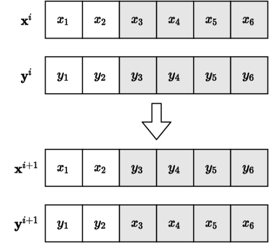
(a) Mate

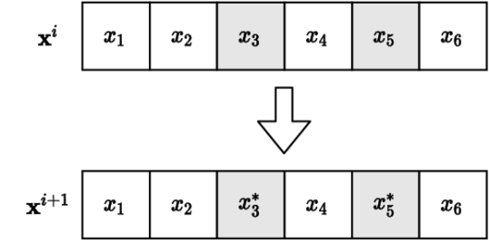
(b) Mutation

Figure 1: Graphical example of mate and mutation where $\mathbf{x}^{i}$ and $\mathbf{y}^{i}$ indicates two generic individuals of the $i$-th generation.

After the mutation step, the fitness of the new individuals is computed and the algorithm restarts with the selection of the best-fit individuals. In this way, the population evolves, generation after generation, towards the optimal individual, avoiding getting blocked in a local minima thanks to the stochastic component introduced by mutation and crossover. Thus, this method is very effective for global optimization where the objective function is potentially non-linear, while standard gradient-based methods can converge to local minima. However GA usually requires an high number of evaluations to perform the optimization, making this procedure very expensive in the case of computational costly objective functions.

3 Active subspaces for minimization on a lower dimensional parameter space

Active Subspaces (AS) [13] method is a dimensionality reduction approach for parameter space studies, which falls under the category of supervised learning techniques. AS tries to reduce the input dimension of a scalar function $f(\bm{\mu}):\Omega\subset\mathbb{R}^{k}\to\mathbb{R}$ by defining a linear transformation $\bm{\mu}_{M}=\mathbf{A}\bm{\mu}$. This method requires the evaluation of the gradients of $f$ since $\mathbf{A}$ depends on the second moment matrix $\mathbf{C}$ of the target function’s gradient, also called uncentered covariance matrix of the gradients of $f$. This matrix is defined as follows

$$\mathbf{C}=\mathbb{E}\,[\nabla_{\bm{\mu}}f\,\nabla_{\bm{\mu}}f^{T}]=\int(\nabla_{\bm{\mu}}f)(\nabla_{\bm{\mu}}f)^{T}\rho\,d\bm{\mu},$$ (1)

where with the symbol $\mathbb{E}[\cdot]$ we denote the expected value, $\nabla_{\bm{\mu}}f\equiv\nabla f({\bm{\mu}})\in\mathbb{R}^{k}$, and $\rho:\mathbb{R}^{k}\to\mathbb{R}^{+}$ is a probability density function which represents the uncertainty in the input parameters. In practice the matrix $\mathbf{C}$ is constructed with a Monte Carlo procedure, and the gradients if not provided can be approximated with different techniques such as local linear models, global models, finite difference, or Gaussian process for example — for a comparison of the methods and corresponding errors the reader can refer to [13, 14, 15]. The uncentered covariance matrix can be decomposed as

$$\mathbf{C}=\mathbf{W}\Lambda\mathbf{W}^{T},$$ (2)

where $\mathbf{W}$ stands for the orthogonal matrix containing the eigenvectors, and $\Lambda$ for the eigenvalues matrix arranged in descending order. The spectral gap [13] is used to bound the error on the numerical approximation with Monte Carlo. We can decompose these two matrices as

$$\Lambda=\begin{bmatrix}\Lambda_{1}&\\ &\Lambda_{2}\end{bmatrix},\qquad\mathbf{W}=\left[\mathbf{W}_{1}\quad\mathbf{W}_{2}\right],\qquad\mathbf{W}_{1}\in\mathbb{R}^{k\times M},$$ (3)

where $M<k$ is the dimension of the active subspace. $M$ should be chosen looking at the energy decay (the tail in the ordered eigenvalue sum) as in POD, or it can be prescribed a priori for the specific task. We can exploit this decomposition to map the input parameters onto a reduced space.

We define the active subspace of dimension $M$ as the principal eigenspace corresponding to the eigenvalues prior to the major spectral gap. We also call the active variable $\bm{\mu}_{M}$ and the inactive variable $\bm{\eta}$. They are defined as $\bm{\mu}_{M}=\mathbf{W}_{1}^{T}\bm{\mu}\in\mathbb{R}^{M}$, and $\bm{\eta}=\mathbf{W}_{2}^{T}\bm{\mu}\in\mathbb{R}^{k-M}$.

In this work we address the constrained global optimization problem of a real-valued continuous function, in the context of genetic algorithms, defined as

$$\min_{\bm{\mu}\in\Omega\subset\mathbb{R}^{k}}f(\bm{\mu}).$$ (4)

To fight the curse of dimensionality and speed up the convergence we exploit the active subspaces property of the target function to select the best individuals in the reduced parameter space, mutate and mate them, and successively to map them in the full parameter space. This translates in the following optimization problem for each generation of individuals:

$$\min_{\begin{subarray}{c}\bm{\mu}_{M}\in\mathcal{P}\subset\mathbb{R}^{M}\\ \bm{\mu}\in\Omega\end{subarray}}\;g(\bm{\mu}_{M}=\mathbf{W}_{1}^{T}\bm{\mu}),$$ (5)

where $\mathcal{P}$ is the polytope in $\mathbb{R}^{M}$ — we assume the ranges of the parameters to be intervals — defined by the AS as $\mathcal{P}:=\{\bm{\mu}_{M}=\mathbf{W}_{1}^{T}\bm{\mu}\;|\;\bm{\mu}\in\Omega\}$. We remark that there are many choices for the profile $g$. In this work we consider the following profile:

$$g(\mathbf{y}):=f(\mathbf{x_{y}})\qquad\forall\mathbf{y}\in\mathcal{Y},$$ (6)

$$\mathcal{Y}:=\{\mathbf{y}\in\mathcal{P}\;|\;\exists\,\mathbf{x_{y}}\in\Omega\,\text{ s.t. }\mathbf{y}=\mathbf{W}_{1}^{T}\mathbf{x_{y}}\}.$$ (7)

We emphasize that the projection map onto the active subspace is a surjective map because $\mathbf{W}_{1}^{T}$ is defined as a linear projection onto a subspace, hence it is surjective by definition. So the back-mapping from the active subspace onto $\Omega$ is not trivial. Given a point $\bm{\mu}_{M}^{*}$ in the active subspace we can find $B$ points in the original parameter space which are mapped onto $\bm{\mu}_{M}^{*}$ by $\mathbf{W}_{1}^{T}$. Recalling the decomposition above we have that

$$\bm{\mu}=\mathbf{W}_{1}\mathbf{W}_{1}^{T}\bm{\mu}+\mathbf{W}_{2}\mathbf{W}_{2}^{T}\bm{\mu}=\mathbf{W}_{1}\bm{\mu}_{M}+\mathbf{W}_{2}\bm{\eta}\qquad\forall\bm{\mu}\in\Omega,$$ (8)

with the additional constraint coming from the rescaling of the input parameters needed to apply AS: $-\mathbf{1}\leq\bm{\mu}\leq\mathbf{1}$, where $\mathbf{1}$ denotes the vector in $\mathbb{R}^{k}$ with all elements equal to $1$. We exploit this to sample the inactive variable $\bm{\eta}$ so that

$$-\mathbf{1}\leq\mathbf{W}_{1}\bm{\mu}_{M}^{*}+\mathbf{W}_{2}\bm{\eta}\leq\mathbf{1},$$ (9)

or equivalently

$$\mathbf{W}_{2}\bm{\eta}\leq\mathbf{1}-\mathbf{W}_{1}\bm{\mu}_{M}^{*}\qquad-\mathbf{W}_{2}\bm{\eta}\leq\mathbf{1}+\mathbf{W}_{1}\bm{\mu}_{M}^{*}.$$ (10)

These inequalities define a polytope in $\mathbb{R}^{k-M}$ from which we want to uniformly sample $B$ points. The inactive variables are sampled from the conditional distribution $p(\bm{\eta}|\bm{\mu}_{M}^{*})$, and we show how to perform it for the uniform distribution. For a more general distribution one should use Hamiltonian Monte Carlo. In particular we start with a simple rejection sampling scheme, which finds a bounding hyperbox for the polytope, draws points uniformly from it, and rejects points outside the polytope. If this method does not return enough samples, we try a hit and run method [46, 6, 34] for sampling from the polytope. This method, starting from the center of the largest hypersphere within the polytope, selects a random direction and identifies the longest segment lying inside the polytope. A new sample is randomly drawn along this segment. The procedure continues starting from the last sample until enough samples are found. If also that does not work, we use $B$ copies of a feasible point computed as the Chebyshev center [7] of the polytope. In fig. 2 we depicted these strategies, at different stages of the sampling.

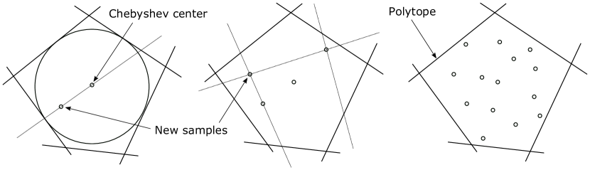
Figure 2: Graphical representation of the inactive variable sampling strategy. We emphasize the Chebyshev center, the selection of the next sample using the hit and run method, and the polytope defined by eq. 10.

4 The proposed ASGA optimization algorithm

In this section we are going to describe the proposed active subspaces extension of the standard GA, named ASGA. Before starting, we emphasize that in what follows, we will maintain the selection, mutation and mate procedures — presented in section 2 — as general as possible, without going into technical details, given the large variety of different options for these steps. In fact the proposed extension is independent on the chosen evolution strategies, and we only perform them in a lower dimension exploiting AS. In algorithm 1 we summarize the standard approach, while in algorithm 2 we highlight the differences introduced by ASGA. We also present an illustration for both the methods in fig. 3, where the yellow boxes indicate the main steps peculiar to ASGA. In both cases, the first step is the generation of the random individuals composing the initial population, and the sequential evaluation of all of them. For ASGA these individuals and their fitness are stored into two additional sets, $\mathbf{X}^{\text{AS}}$ for the individuals, and $\mathbf{y}^{\text{AS}}$ for the fitness. We will exploit them as input-output pair for the construction of the AS. After the selection of the best-fit individuals, the active subspace of dimension $M$ is built and the selected offspring is projected onto it. The low-dimensional individuals mate and mutate in the active subspace. Thanks to the reduced dimension and to the fact that we retain only the most important dimensions, these operations are much more efficient. Thus, even if the AS of dimension $M$ does not provide an accurate approximation of the original full-dimensional space, the active dimensions will provide preferential directions for the evolution, making the iterative process smarter and faster.

Figure 3: Active subspaces-based genetic algorithm scheme. The main step of the classical GA are depicted from top to bottom. The yellow boxes represent projections onto and from lower dimension active subspace, which are specific to ASGA.

After the evolution, the low-dimensional offspring is mapped back to the original space. In section 3 we describe how for any point in the active subspace we can find several points in the original space which are mapped onto it. So we select, for any individual in the offspring, $B$ full-dimensional points which correspond to the individual in the active subspace. We emphasize that to preserve the same dimensionality of the offspring between the original GA and the AS extension, in the proposed algorithm we select the $\nicefrac{{N}}{{B}}$ best individuals, instead of selecting $N$. In this way, after the back-mapping, the offspring has dimension $N$ in both versions. The number of back-mapped points $B$, and the active subspace dimension $M$ — that can be a fixed parameter or dynamically selected from the spectral gap of the covariance matrix $\mathbf{C}$ — represent the new (hyper-)parameters of the proposed method.

Finally the fitness of the new individuals, now in the full-dimensional space, are evaluated. To make the AS more precise during the iterations, the evaluated individuals and their fitness are added to $\mathbf{X}^{\text{AS}}$ and $\mathbf{y}^{\text{AS}}$. The process restarts from the selection of the offspring from the new generation, continuing as described above until the stopping criteria are met.

We stress on the fact that the structure of the algorithm is similar to the original GA approach, with the difference that the gradients at the sample points are approximated in order to identify the dimensions with highest variance. Even if such information about the function gradient is used, the ASGA method is different from gradient-based methods: numerically computing the gradient with a good accuracy at a specific point — that is the fundamental step of gradient-based methods to move on the solution manifold — is a very expensive procedure, especially in a high-dimensional space. In ASGA we avoid such computation, exploiting instead the already collected function evaluations. Further, gradient-based techniques converges (relatively) fast to optimum, but they get blocked into local minima, contrarily to the ASGA approach. It is important to remark that, for each generation, the AS is rebuilt from scratch, losing efficiency but gaining more precision due to the growing number of elements in the two sets $\mathbf{X}^{\text{AS}}$ and $\mathbf{y}^{\text{AS}}$. We also remark the samples are generated with a uniform distribution only at the first generation. After that, due to the ASGA steps the distribution changes in a way which can not be known a priori. For the computation of the expectation operator in eq. 1 in this work we assume a uniform distribution. Even if this may introduce an unknown error, the numerical results achieved by ASGA seem to support such choice. Of course the numerical estimates present in the literature for the uniform distribution do not apply in such case. This method can be viewed as an active learning procedure in a Bayesian integration context, where the maximized acquisition function is heuristic and given by the application of AS and GA steps. Another interpretation is that we are enriching the local informations near the current minimum to feed the AS algorithm, so it can be viewed as a weighted AS.

Algorithm 1 Standard GA.

Input:
           initial population size $N_{0}$
           population size $N$


           selection routine select
           mutation routine mutate
           mate routine mate
           objective function fobj
           stop criteria
      Output:
           final population $\mathbf{X}^{\text{end}}$

1:procedure GeneticAlgorithm

2:    $g\leftarrow$ 0

3:    $\mathbf{X}^{g}\leftarrow$ random pop of size $N_{0}$

4:    $\mathbf{y}^{g}\leftarrow$ fobj($\mathbf{X}^{g}$)    

5:    repeat

6:       $g\leftarrow g+1$

7:       $\mathbf{X^{*}}\leftarrow$ select($\mathbf{X}^{g-1},\mathbf{y}^{g-1},N$)    

8:       $\mathbf{X^{*}}\leftarrow$ mate($\mathbf{X}^{*}$)

9:       $\mathbf{X}^{g}\leftarrow$ mutate($\mathbf{X}^{*}$)          

10:       $\mathbf{y}^{g}\leftarrow$ fobj($\mathbf{X}^{g}$)    

11:    until stop criteria reached

12:    $\mathbf{X}^{\text{end}}\leftarrow\mathbf{X}^{g}$

13:    return $\mathbf{X}^{\text{end}}$

14:end procedure

Algorithm 2 Proposed ASGA.

Input:
           initial population size $N_{0}$
           population size $N$
           active dimension $M$
           number backward $B$
           selection routine select
           mutation routine mutate
           mate routine mate
           objective function fobj
           stop criteria
      Output:
           final population $\mathbf{X}^{\text{end}}$

1:procedure ASGA

2:    $g\leftarrow$ 0

3:    $\mathbf{X}^{g}\leftarrow$ random pop of size $N_{0}$

4:    $\mathbf{y}^{g}\leftarrow$ fobj($\mathbf{X}^{g}$)

5:    $\mathbf{X}^{\text{AS}}\leftarrow\mathbf{X}^{g}$

6:    $\mathbf{y}^{\text{AS}}\leftarrow\mathbf{y}^{g}$

7:    repeat

8:       $g\leftarrow g+1$

9:       $\mathbf{X^{*}}\leftarrow$ select($\mathbf{X}^{g-1},\mathbf{y}^{g-1},{\color[rgb]{0,0,0}\textstyle\frac{N}{B}}$)

10:       build AS($\mathbf{X}^{\text{AS}},\mathbf{y}^{\text{AS}},M$)

11:       $\mathbf{X}_{M}^{*}\leftarrow$ forward($\mathbf{X}^{*}$)

12:       $\mathbf{X}_{M}^{*}$ $\leftarrow$ mate($\mathbf{X}_{M}^{*}$)

13:       $\mathbf{X}_{M}^{*}$ $\leftarrow$ mutate($\mathbf{X}_{M}^{*}$)

14:       for $\mathbf{x}$ in $\mathbf{X}_{M}^{*}$ do

15:          for $i\leftarrow 1$ to $B$ do

16:             $\mathbf{X}^{g}\leftarrow$ backward($\mathbf{x}$)

17:          end for

18:       end for

19:       $\mathbf{y}^{g}\leftarrow$ fobj($\mathbf{X}^{g}$)

20:       $\mathbf{X}^{\text{AS}}\leftarrow\mathbf{X}^{\text{AS}}\cup\mathbf{X}^{g}$

21:       $\mathbf{y}^{\text{AS}}\leftarrow\mathbf{y}^{\text{AS}}\cup\mathbf{y}^{g}$

22:    until stop criteria reached

23:    $\mathbf{X}^{\text{end}}\leftarrow\mathbf{X}^{g}$

24:    return $\mathbf{X}^{\text{end}}$

25:end procedure

5 Numerical results

In this section we are going to present the results obtained by applying the proposed algorithm, firstly to some test functions that are usually used as benchmarks for optimization problems. Since this method is particularly suited for high-dimensional functions, we analyze the optimization convergence for three different input dimension ($2$, $15$, and $40$), i.e. the number of genes of each individual. The second test case we propose is instead a typical engineering problem, where we optimize the lift-to-drag coefficient of a NACA airfoil which is deformed using a map $\mathcal{M}:\mathbb{R}^{10}\to\mathbb{R}$ defined in section 5.2. In this example we opted for the use of a surrogate model only to evaluate the individuals’ fitness for computational considerations, since we just want to compare ASGA with GA. We do not rely on the surrogate for the gradients approximation. In [18], instead, we apply ASGA on a naval engineering hydrodynamics problem, where we do not rely on a surrogate model of the target function, but instead we exploit data-driven model order reduction methods to reconstruct the fields of interest and then compute the function to optimize.

In both the test cases, in order to collect a fair comparison, we adopt the same routines for the selection, the mutation and the crossover steps. In particular:

• for the mate we use the blend BLX-alpha crossover [25] with $\alpha=1.0$, with a mate probability of $50\%$. With this method, the offspring results:

  $$\begin{cases}{\color[rgb]{0,0,0}\mathbf{x}_{a}^{i}}=(1-\gamma){\color[rgb]{0,0,0}\mathbf{x}_{a}^{i-1}}+\gamma{\color[rgb]{0,0,0}\mathbf{x}_{b}^{i-1}}\\ {\color[rgb]{0,0,0}\mathbf{x}_{b}^{i}}=\gamma{\color[rgb]{0,0,0}\mathbf{x}_{a}^{i-1}}+(1-\gamma){\color[rgb]{0,0,0}\mathbf{x}_{b}^{i-1}}\end{cases}\quad\text{for}\;{\color[rgb]{0,0,0}a,b}=1,\dotsc,N,$$ (11)

  where ${\color[rgb]{0,0,0}\mathbf{x}_{a}^{i-1}}$ and ${\color[rgb]{0,0,0}\mathbf{x}_{b}^{i-1}}$ refer to the parent individuals (at the $i-1$th generation), ${\color[rgb]{0,0,0}\mathbf{x}_{a}^{i}}$ and ${\color[rgb]{0,0,0}\mathbf{x}_{b}^{i}}$ are the mated individuals, $N$ is the cardinality of population, and $\gamma$ is a random variable chosen in the interval $[-\alpha,1+\alpha)$. We mention that eq. 11 can recover the graphical description of mating in fig. 1(a) if $\gamma$ is taken to be discrete, either $0$ or $1$, and applied component-wise.

• for the mutation, a Gaussian operator [28] has been used with a mutation probability of $50\%$. This strategy changes genes by adding a normal noise. Since we do not have any knowledge about the low-dimensional space, tuning the variance of such mutation may result in a not trivial procedure. This quantity has in fact to be set in order to explore the input space but, as the same time, producing minimal differences between parents and offspring. A fixed variance for both the spaces may cause a too big distance — in $l_{2}$ sense — between parents and offspring, inhibiting the convergence. To overcome this potential problem, we correlate the Gaussian variance with the genes theirselves, ensuring a reasonable mutation in both spaces. The adopted mutation method is:

  $${\color[rgb]{0,0,0}\mathbf{x}_{a}^{i}}={\color[rgb]{0,0,0}\mathbf{x}_{a}^{i-1}}+\varepsilon\,{\color[rgb]{0,0,0}\mathbf{x}}_{a}^{i-1}\qquad\text{for}\;{\color[rgb]{0,0,0}a}=1,\dots,N,$$ (12)

  where $\varepsilon$ is a random variable with probability distribution $\mathcal{N}(\mu,\sigma^{2})$, that is $\varepsilon\sim\mathcal{N}(\mu,\sigma^{2})$, with $\mu=0$ and $\sigma^{2}=0.1$.

Regarding the selection, since the limited number of individuals per population, we adopt one of the simplest criteria, by selecting the $N$ best individuals in terms of fitness.

We also keep fixed the additional parameters for the AS extension: the number of active dimensions $M$ is set to $1$, while the number of back-mapped points is $2$. All the gradients computations are done using local linear models. For the actual computation regarding AS we used the ATHENA Python package [41]. The only varying parameters are the size of the initial population $N_{0}$, the size of population during the evolution $N$, and the number of generations in the evolutive loop, which are chosen empirically based on the objective function. We emphasize that, due to the stochastic nature of these methods, we repeated the tests $15$ times, with different initial configurations, presenting the mean value, the minimum and the maximum over the $15$ runs.

5.1 Benchmark test functions

We applied the optimization algorithm to $6$ different $n$-dimensional test functions, which have been chosen to cover a large variety of possible shapes. For all the functions, the results of the proposed method are compared to the results obtained using the standard genetic approach. In detail, the functions we tested are the so called: Rosenbrock, Ackley, Bohachevsky, Rastrigin, Schaffer N. 7 and Zakharov. In Figure 4 we depict the test functions, in their two-dimensional form. In the following paragraphs we briefly introduce them before presenting the obtained results. For a complete literature survey on benchmark functions for global optimization problems we suggest [31].

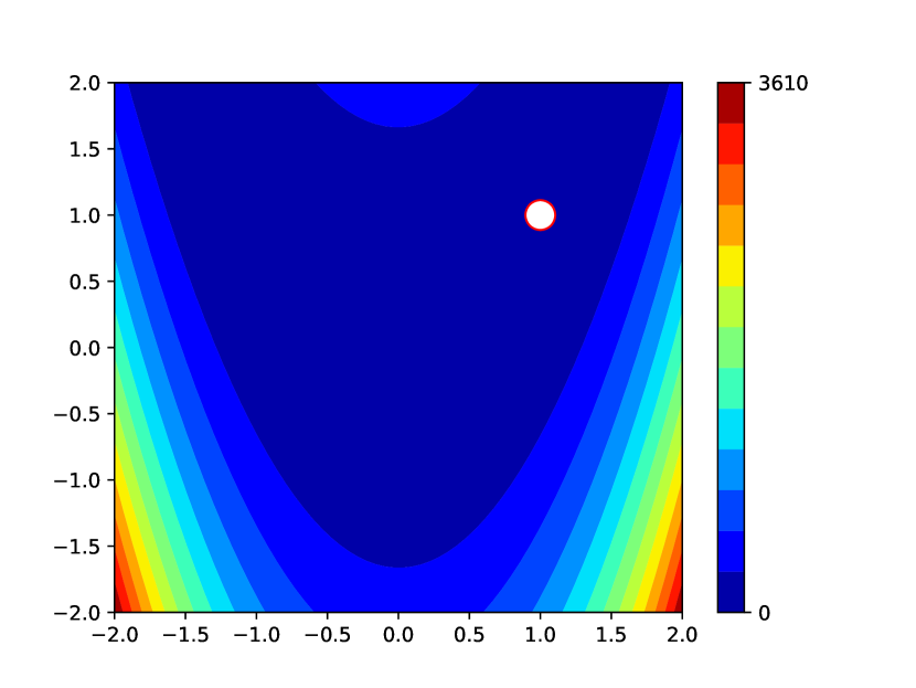
(a) Rosenbrock function.

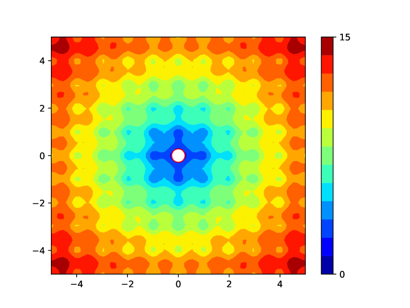
(b) Ackley function.

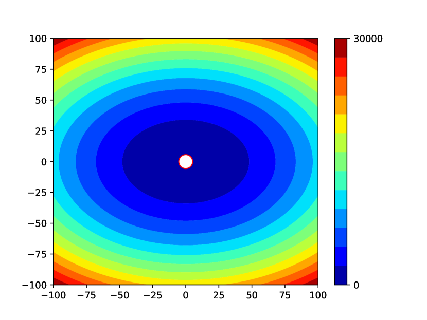
(c) Bohachevsky function.

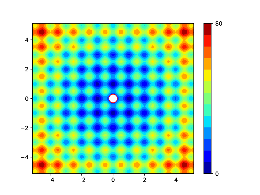
(d) Rastrigin function.

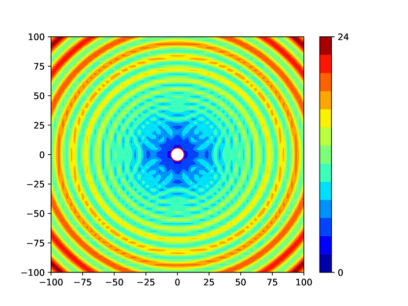
(e) Schaffer N. 7 function.

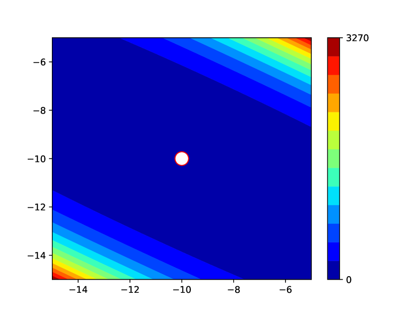
(f) Zakharov function.

Figure 4: Benchmark test functions representation in 2D. White dots indicate the global minima.

(a) Rosenbrock function

The Rosenbrock function is a widespread test function in the context of global optimization [20, 5, 38]. We choose it as representative of the valley-shaped test functions. The general $d$-dimensional formulation is the following:

$$f(x)=\sum_{i=1}^{d-1}[100(x_{i+1}-x_{i}^{2})^{2}+(x_{i}-1)^{2}].$$ (13)

Its global minimum is $f(x^{*})=0$, at $x^{*}=(1,1,\dots,1)$. As we can see from fig. 4(a) the minimum lies on a easy to find parabolic valley, but the convergence to the actual minimum is notoriously difficult. We evaluated the function in the hypercube $[-5,10]^{d}$.

(b) Ackley function

The Ackley function is characterized by many local minima making it difficult to find the global minimum, especially for hillclimbing algorithms [4, 2]. The general $d$-dimensional formulation is the following:

$$f(x)=-a\exp\left(-b\sqrt{\frac{1}{d}\sum_{i=1}^{d}x_{i}^{2}}\right)-\exp\left(\sqrt{\frac{1}{d}\sum_{i=1}^{d}\cos(cx_{i})}\right)+a+\exp(1),$$ (14)

where $a$, $b$, and $c$ are set to $20$, $0.2$, and $2\pi$, respectively. Its global minimum is $f(x^{*})=0$, at $x^{*}=(0,0,\dots,0)$. As we can see from fig. 4(b) the function is nearly flat in the outer region, with many local minima, and the global minimum lies on a hole around the origin. The function has been evaluated in the domain $[-15,30]^{d}$.

(c) Bohachevsky function

The Bohachevsky function is a representative of the bowl-shaped functions. There are many variants and we chose the general $d$-dimensional formulation as the following:

$$f(x)=\sum_{i=1}^{d-1}(x_{i}^{2}+2x_{i+1}^{2}-0.3\cos(3\pi x_{i})-0.4\cos(4\pi x_{i+1})+0.7).$$ (15)

Its global minimum is $f(x^{*})=0$, at $x^{*}=(0,0,\dots,0)$. As we can see from fig. 4(c) the function has a clear bowl shape. This function has been evaluated in the domain $[-100,100]^{d}$.

(d) Rastrigin function

The Rastrigin function is another difficult function to deal with for global optimization with genetic algorithm due to the large search space and its many local minima [36]. The general $d$-dimensional formulation is the following:

$$f(x)=10d+\sum_{i=1}^{d}[x_{i}^{2}-10\cos(2\pi x_{i})].$$ (16)

Its global minimum is $f(x^{*})=0$, at $x^{*}=(0,0,\dots,0)$. As we can see from fig. 4(d) the function is highly multimodal with local minima regularly distributed. We evaluated this function in the input domain $[-5.12,5.12]^{d}$.

(e) Schaffer N. 7 function

The Schaffer N. 7 function [44] is a stretched V sine wave. The general $d$-dimensional formulation is the following:

$$f(x)=\sum_{i=1}^{d-1}(x_{i}^{2}+x_{i+1}^{2})^{0.25}\left[\sin^{2}(50(x_{i}^{2}+x_{i+1}^{2})^{0.10})+1\right].$$ (17)

Its global minimum is $f(x^{*})=0$, at $x^{*}=(0,0,\dots,0)$. As we can see from fig. 4(e) the function presents many local minima. The optimization has been performed in the hypercube $[-100,100]^{d}$.

(f) Zakharov function

The Zakharov function is a representative of the plate-shaped functions. It has no local minima and one global minimum. The general $d$-dimensional formulation is the following (after a shift):

$$f(x)=\sum_{i=1}^{d}(x_{i}+10)^{2}+\left(\sum_{i=1}^{d}\frac{i}{2}(x_{i}+10)\right)^{2}+\left(\sum_{i=1}^{d}\frac{i}{2}(x_{i}+10)\right)^{4}.$$ (18)

We emphasize that we used a shifted version with global minimum $f(x^{*})=0$, at $x^{*}=(-10,-10,\dots,-10)$. This choice is made to prove that the proposed method is not biased towards minima around the origin. We can see from fig. 4(f) the function for $d=2$. We evaluated the Zakharov function in the domain $[-15,0]^{d}$.

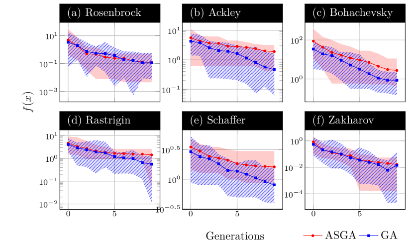
Figure 5: Results of the optimization of the benchmark functions in a space of dimension $d=2$. We compare the standard GA (in blue square dots) with the proposed algorithm ASGA (in red circle dots) using an initial population of size $30$, while the dimension for each generation is fixed to $10$. The solid lines represent the mean, over $15$ runs, of the objective function corresponding to the best individual at each generation. The shaded areas show the interval between minimum and maximum (blue with lines for GA, red for ASGA).

All the test cases presented share the same hyper-parameters described at the beginning of this section, except for the population size. For the $2$-dimensional benchmark functions, the two algorithms are tested creating $N_{0}=200$ random individuals for the initial population, then keeping an offspring of dimension $N=100$. The fig. 5 shows the behaviour for all the test functions. For this space dimension, the two trends are very similar: the usage of the proposed algorithm does not make the optimization faster, and adds the computational overhead for the AS construction. Despite that, the results after $10$ generations are very similar, and we can consider this as a worst case scenario, where a clear reduction in the parameter space is not possible.

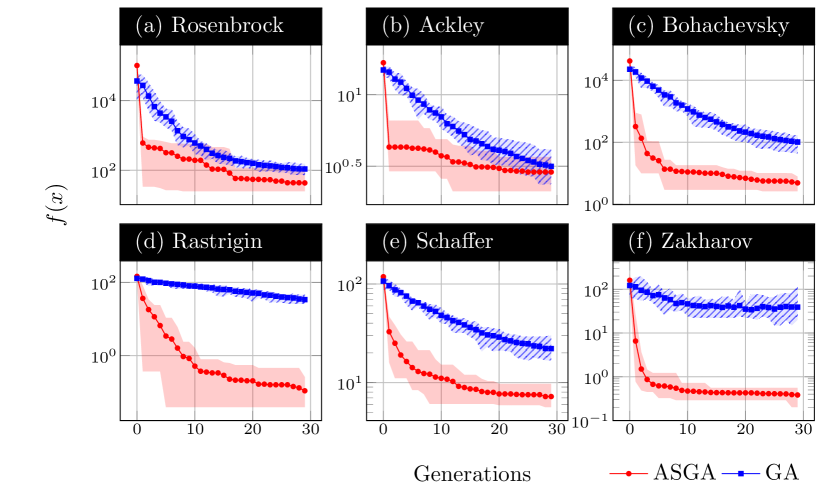
Figure 6: Results of the optimization of the benchmark functions in a space of dimension $d=15$. We compare the standard GA (in blue square dots) with the proposed algorithm ASGA (in red circle dots) using an initial population of size $2000$, while the dimension for each generation is fixed to $200$. The solid lines represent the mean, over $15$ runs, of the objective function corresponding to the best individual at each generation. The shaded areas show the interval between minimum and maximum (blue with lines for GA, red for ASGA).

The ASGA performance gain changes drastically increasing the number of dimension to $d=15$, as demonstrated in fig. 6. For such dimension, the two parameters $N_{0}$ and $N$ are set to $2000$ and $200$, respectively. Starting from this dimension, it is possible to note a remarkable difference between the standard method and the proposed one. The greater the input dimension, the greater the gain produced by ASGA, due to the exploitation of the AS reduction. All the benchmarks show a faster decay, but we can isolate two different patterns in the evolution: Rosenbrock and Ackley show a very steep trend in the first generation gain, while for the next generations the population is not able to decrease its fitness as much as before, showing a quasi-constant behaviour. The difference with the standard genetic algorithm is maximized in the first generation, but even if the evolution using ASGA is not so effective after the first generation in these two cases, the proposed method is able to achieve anyway a better result (on average) after $30$ generations. The other benchmarks instead show a much smoother decay, gradually converging to the optimum. Despite the lack of the initial step, for these benchmarks the gain with respect to the standard approach becomes bigger, even if after several generations the convergence rate decreases.

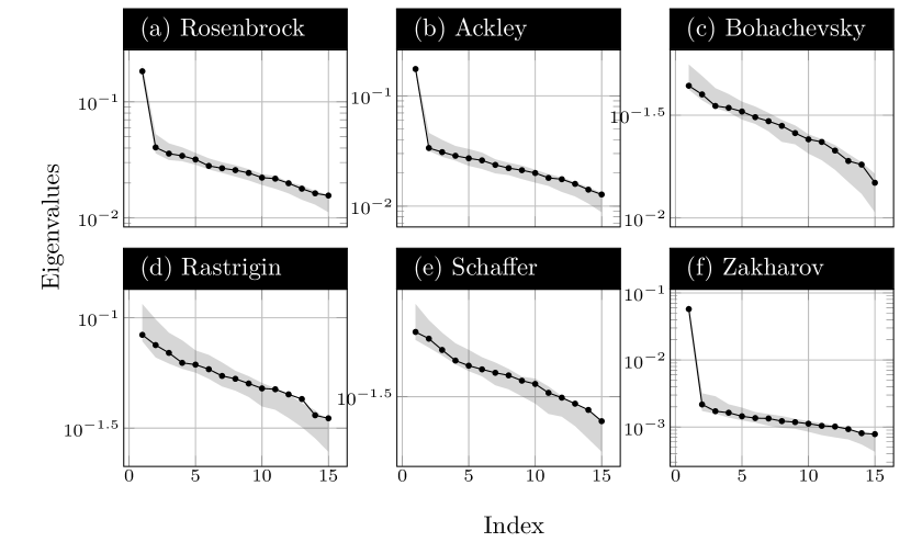
Figure 7: Eigenvalues estimates of the matrix $\mathbf{C}$ in eq. 1 for all the benchmarks, at the first generation, for $d=15$. The black dots in the plot indicate the eigenvalues, while the grey area is defined by the bootstrap intervals.

In order to better understand these differences, we investigate the spectra of the AS covariance matrices for all the benchmarks, which are reported in fig. 7. The patterns individuated in the optimizations are partially reflected in the eigenvalues: Rosenbrock, Ackley and Zakharov have an evident gap between the first and the second eigenvalues, which results in a better approximation (of the original function) in the $1$-dimensional subspace. However, the order of magnitude of the first eigenvalue is different between the three functions: for Rosenbrock and Ackley the magnitude is greater than $0.1$ whereas for Zakharov is around $0.05$.

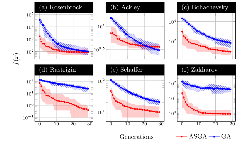
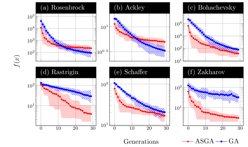
Figure 8: Results of the optimization of the benchmark functions in a space of dimension $d=15$, with active dimension $M=2$ (top) and $M=5$ (bottom). We compare the standard GA (in blue square dots) with the proposed algorithm ASGA (in red circle dots) using an initial population of size $2000$, while the dimension for each generation is fixed to $200$. The solid lines represent the mean, over $15$ runs, of the objective function corresponding to the best individual at each generation. The shaded areas show the interval between minimum and maximum (blue with lines for GA, red for ASGA).

Since for all the tests, the ASGA approach performs better than its classical counterpart despite the absence, in some cases, of an evident spectral gap in the AS covariance matrix, we perform further investigations. In particular, we use the same tests as before ($15$-dimensional functions) but with a different number of active dimensions, i.e. $M=\{2,5\}$, instead of $M=1$. In fig. 8 we show the comparison between the classical GA and the ASGA outcomes. It is possible to note that by increasing the active dimension, the differences between the performances of the two methods become smaller. Only for the Rosenbrock and for the Ackley functions we can see that ASGA with $M=5$ is not able to reach the same order of magnitude reached by GA (we remark the original space has dimension $d=15$).

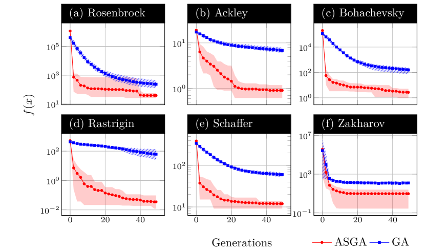
Figure 9: Results of the optimization of the benchmark functions in a space of dimension $d=40$. We compare the standard GA (in blue square dots) with the proposed algorithm ASGA (in red circle dots) using an initial population of size $5000$, while the dimension for each generation is fixed to $1000$. The solid lines represent the mean, over $15$ runs, of the objective function corresponding to the best individual at each generation. The shaded areas show the interval between minimum and maximum (blue with lines for GA, red for ASGA).

Increasing the input dimension to $d=40$ shows a much clearer benefit in using the proposed method, as we can see in fig. 9. Here we set $N_{0}=5000$ and $N=1000$. We specify that we set the active dimension $M=1$. Also with this dimensionality, we are able to isolate two main behaviours in the convergence of the six benchmarks: a very steep trend in the first generation, and a more smooth one, but still equally effective. The interesting thing is that some benchmarks do not reflect the behaviour collected with $d=15$. While Rosenbrock, Rastrigin and Zakharov show a similar convergence rate for ASGA, the other benchmarks present a change in the slope. The different behaviours observed for the same benchmarks evaluated at different input dimensional spaces is due to the fact that the method is sensitive to the approximation accuracy of the gradients of the model function with respect to the input data. This is an issue inherited by the application of AS. Moreover, since we are keeping just one active variable, we are discarding several information, thus the representation of the function along the active subspace could present some noise. So the genetic procedure enhanced by AS is able to converge fast to the optimum, but this optimum may be — for the space simplification — distant to the true optimum. From the tests with higher active dimension, we note that the improvement in the first iterations is not as rapid as by using a $1$-dimensional AS. Also, keeping more active dimensions, the performance of ASGA becomes similar to the standard GA. We can conclude that with one (or few) active dimension, ASGA reaches the global minimum with less function evaluations, but we get stuck with the projection error introduced by AS, whereas by increasing the active dimension we reduce the projection error but we lose the effectiveness of the evolution steps in a reduced space. A possible solution for this problem can be a smarter (and dynamical) strategy to select the number of active dimensions.

Over all the three test cases, where we vary the input space dimension, the performance of ASGA are better or equal than the standard GA. In table 1 we summarize the relative gain on average achieved after the entire evolution and after only one generation, divided by test function, both with the GA and ASGA methods. The relative gain is computed as the mean over $15$ runs of the ratio between the objective function evaluated at the best-fit individual at the beginning of the evolution ($f(x_{\text{opt}}^{0})$) and the objective function evaluated at the best-fit individual after $k$ generations, with $k=1$ and $k=N_{\text{gen}}$, where $N_{\text{gen}}$ is the maximum number of generations depending on the input dimension. This relative gain $G(k)$ reads,

$$G(k)=\frac{1}{15}\sum_{i=1}^{15}f(x_{\text{opt}_{i}}^{0})/f(x_{\text{opt}_{i}}^{k}),$$ (19)

where $x_{\text{opt}_{i}}^{k}$ is the best-fit individual of the population at the $i$-th run and at $k$-th generation. Highest values correspond to a more effective optimization, and for dimensions $15$ and $40$ we can see from table 1 that ASGA performs better than standard GA for all the benchmarks. Even the gain after just one evolutive iteration is bigger in all the collected tests, reaching in some cases some order of magnitude of difference with respect to GA. These results suggest that despite the computational overhead for the construction of AS and the back-mapping, an application of the ASGA over the standard GA produces usually better or at least comparable results for a fixed generation.

Table 1: Summary comparison between GA and ASGA with respect to the gain $G(k)$ defined in eq. 19. We compare the gain for the first and for the last generation.

Function	Method	dim = 2		dim = 15		dim = 40
		$G(9)$	$G(1)$	$G(29)$	$G(1)$	$G(49)$	$G(1)$
	GA	9.17	1.13	4.71	1.03	2.53	1.10
Ackley	ASGA	2.93	1.29	5.81	3.89	20.91	3.00
	GA	39.58	1.78	223.86	1.22	729.05	1.81
Bohachevsky	ASGA	31.66	2.04	8608.41	130.72	75104.33	3548.70
	GA	7.34	1.41	3.80	1.05	6.97	1.17
Rastrigin	ASGA	3.24	1.39	1343.41	4.00	14738.40	71.77
	GA	30.04	1.74	335.33	1.34	1723.89	2.42
Rosenbrock	ASGA	39.68	2.66	2343.57	167.48	29747.56	1600.24
	GA	3.64	1.21	4.83	1.11	5.66	1.18
Schaffer	ASGA	2.16	1.17	16.41	3.61	32.57	10.38
	GA	38.59	2.65	3.11	1.07	2148.39	26.50
Zakharov	ASGA	51.14	3.88	417.86	24.46	37739.61	237.48

5.2 Shape design optimization of a NACA airfoil

Here we present the shape design optimization of a NACA 4412 airfoil [1]. Since the purpose of this work is limited to the extension of the GA, we briefly present the details of the complete model, with a quick overview of the application. To reproduce the full order simulations please refer to [51].

Let be given the unsteady incompressible Navier-Stokes equations described in an Eulerian framework on a parametrized space-time domain $Q(\bm{\mu})=\Omega\times[0,T]\subset\mathbb{R}^{d}\times\mathbb{R}^{+}$, $d=2,3$ with the velocity field denoted by $\mathbf{u}:Q(\bm{\mu})\to\mathbb{R}^{d}$, and the pressure field by $p:Q(\bm{\mu})\to\mathbb{R}$, such that:

$$\begin{cases}\mathbf{u_{t}}+\mathbf{\nabla}\cdot(\mathbf{u}\otimes\mathbf{u})-\mathbf{\nabla}\cdot 2\nu\mathbf{\nabla^{s}}\mathbf{u}=-\mathbf{\nabla}p&\mbox{ in }Q(\bm{\mu}),\\ \mathbf{\nabla}\cdot\mathbf{u}=\mathbf{0}&\mbox{ in }Q(\bm{\mu}),\\ \mathbf{u}(t,x)=\mathbf{f}(\mathbf{x})&\mbox{ on }\Gamma_{\text{in}}\times[0,T],\\ \mathbf{u}(t,x)=\mathbf{0}&\mbox{ on }\Gamma_{0}(\bm{\mu})\times[0,T],\\ (\nu\nabla\mathbf{u}-p\mathbf{I})\mathbf{n}=\mathbf{0}&\mbox{ on }\Gamma_{\text{out}}\times[0,T],\\ \mathbf{u}(0,\mathbf{x})=\mathbf{k}(\mathbf{x})&\mbox{ in }Q(\bm{\mu})_{0},\\ \end{cases}$$ (20)

holds. Here, we have that $\Gamma=\Gamma_{\text{in}}\cup\Gamma_{0}\cup\Gamma_{\text{out}}$ is the boundary of $\Omega$ and it is composed by the inlet boundary $\Gamma_{\text{in}}$, the outlet boundary $\Gamma_{\text{out}}$ and the physical walls $\Gamma_{0}(\bm{\mu})$. The term $\mathbf{f}(\mathbf{x})$ stands for the stationary non-homogeneous boundary condition, whereas $\mathbf{k}(\mathbf{x})$ indicates the initial condition for the velocity at $t=0$. Shape changes are applied to the boundary $\Gamma_{0}(\bm{\mu})$ corresponding to the airfoil wall, which in the undeformed configuration corresponds to the 4-digits, NACA 4412 wing profile. Such shape modifications are associated to numerical parameters contained in the vector $\bm{\mu}\in\mathbb{R}^{k}$ with $k=10$.

As geometrical deformation map $\mathcal{M}$ we adopt the shape morphing proposed in [27], where 5 shape functions $r_{i}$ are added to the upper and lower part of the airfoil profile denoted by $y^{+}$ and $y^{-}$, respectively. Each shape function is multiplied by a possible different coefficient as in the following

$$y^{+}=\overline{y^{+}}+\sum_{i=1}^{5}a_{i}r_{i},\qquad y^{-}=\overline{y^{-}}-\sum_{i=1}^{5}b_{i}r_{i},$$ (21)

where the bar denotes the reference undeformed profile. These $10$ coefficients ($a_{i}$ and $b_{i}$) represent the input parameters $\bm{\mu}\in\mathbb{D}:=[0,0.03]^{10}$. In fig. 10 we depict the NACA 4412 together with the $5$ rescaled shape functions $r_{i}$. The output function we want to maximize is the lift-to-drag coefficient, one of the typical quantities of interest in aeronautical problems. To recast the problem in a minimization setting, we just minimize the opposite of the coefficient. To compute it, we model a turbulent flow pasting around the 2D airfoil using the incompressible Reynolds Averaged Navier–Stokes equations. Regarding the main numerical settings, we adopt a finite volume approach with the Spalart–Allmaras model, with a computational grid of $46500$ degrees of freedom. The flow velocity, at the inlet boundary, is set to $1$ m/s, while the Reynolds number is fixed to $50000$. For the detailed problem formulation we refer to the experiments conducted in [51].

Instead of running the high-fidelity solver for any new untested parameter, we optimize a RBF response surface built using the initial dataset. Due to the stochastic nature of the method, also in this test case we test the methods for several initial settings — $25$ different runs — making the total computational load very high. Thus, we decided to build a response surface using a dataset of $333$ samples, computed with the numerical scheme described above, mimicking at the same time a typical industrial workflow.

The objective function $f_{\text{o}bj}(\bm{\mu}):\mathbb{D}\subset\mathbb{R}^{10}\to\mathbb{R}$ we are going to minimize is the following:

$$f_{\text{o}bj}(\bm{\mu})=\begin{cases}g(\bm{\mu})\quad\text{if }\,\bm{\mu}\in\mathbb{D},\\ \alpha\quad\quad\,\,\text{if }\,\bm{\mu}\notin\mathbb{D},\\ \end{cases}$$ (22)

where $g(\bm{\mu})$ is the response surface built using the radial basis function (RBF) interpolation technique [9] over the samples, while $\alpha\in\mathbb{R}$ is a penalty constant. To prevent the evolution from creating new individuals that do not belong to $\mathbb{D}$, we impose a penalty factor $\alpha=10$. We recall that we minimize the opposite of the lift-to-drag coefficient.

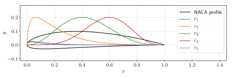
Figure 10: NACA 4412 profile with the $5$ shape functions $r_{i}$ rescaled by a factor equal to $0.2$.

fig. 11 reports the evolution of the best-fit individual over $10$ generations. Also in this case, we apply the proposed algorithm and the standard GA to $25$ different initial settings, using an initial population size $N_{0}=20$ and selecting at each generations the $N=10$ best-fit individuals for the offspring. The plot depicts the mean best-fit individual with solid lines, whereas the shaded areas show the interval between the minimum and maximum (of the $25$ runs) for each generation. Even if the dimension of the parameter space is not very high ($10$), we can see that on average the proposed algorithm is able to converge faster. The difference between the two methods is not as remarkable as in a higher dimensional test case, but we can see that the best run using standard GA is slightly worse than the mean optimum achieved by ASGA. This again demonstrates the value in the proposed method. Moreover, we emphasize that also in this case the decay of the objective function in the first generations with ASGA is faster.

Figure 11: Results of the optimization of the NACA airfoil design in a $10$-dimensional space. We compare the standard GA (in blue square dots) with the proposed algorithm ASGA (in red circle dots) using an initial population of size $20$, while the dimension for each generation is fixed to $10$. The solid lines represent the mean, over $25$ runs, of the objective function corresponding to the best individual at each generation. The shaded areas show the interval between minimum and maximum (blue with lines for GA, red for ASGA).

6 Conclusions

In this work, we have presented a novel approach for optimization problems coupling the supervised learning technique called active subspaces (AS) with the standard genetic algorithm (GA). We have demonstrated the benefits of such method by applying it to some benchmark functions and to a realistic engineering problem. The proposed method achieves faster convergence to the optimum, since the individuals evolve only along few principal directions (discovered exploiting the AS property). Further, from the results it emerges that the gain induced from the ASGA method is greater for high-dimensionality functions, making it particularly suited for models with many input parameters.

This new method can also be integrated in numerical pipelines involving model order reduction and reduction in parameter space. Reducing the number of input parameters is a key ingredient to improve the computational performance and to allow the study of very complex systems.

Since the number of active dimensions is important for the accuracy of the AS, future developments will focus on an efficient criterion to select dynamically the number of AS dimensions, which in the presented results are kept fixed. Future studies will also address the problem of incorporating non-linear extensions of active subspaces into the ASGA, focusing on the construction of a proper back-mapping from the reduced space to the original full parameter space.

Appendix A On ASGA convergence

The aim of this section is to provide further insights about the convergence of the ASGA method. We perform a single run on all the benchmark functions presented above, in a space of dimension $d=2$. We kept unaltered all the ASGA numerical settings described in section 5, so for all the details we refer to such section. We emphasize that we used the same hyper-parameters of the $2$-dimensional optimization test, except for the number of generations which we increased to $100$.

We summarize in fig. 12 and fig. 13 the spatial coordinates of the best individual after each generation using the standard GA and ASGA. The proposed method reaches the global minimum for all the testcases, performing better than the standard counterpart for the Rosenbrock and Rastrigin functions.

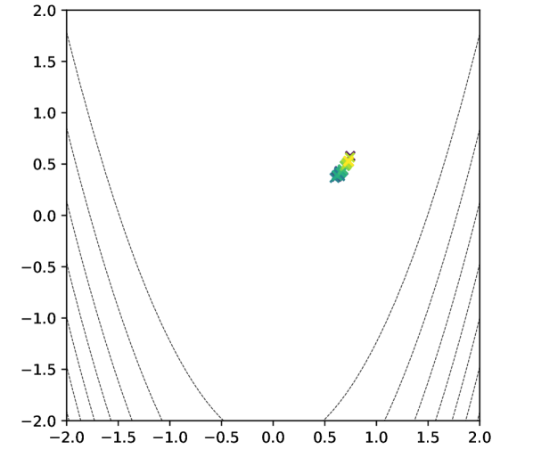
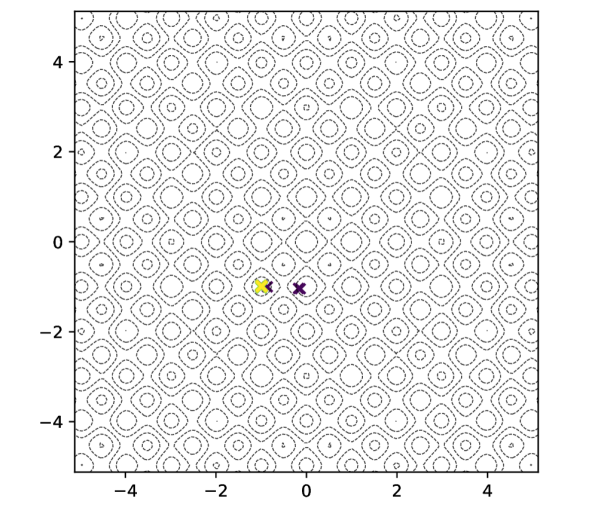
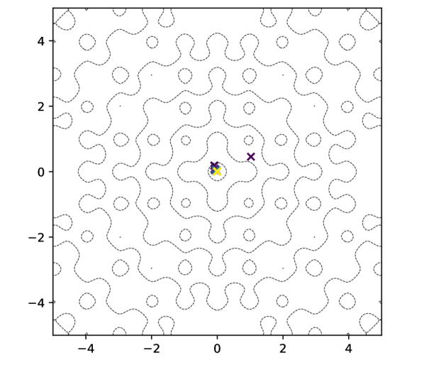
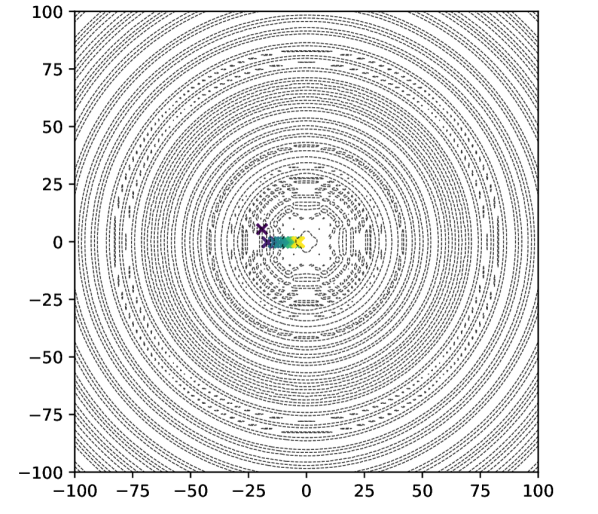
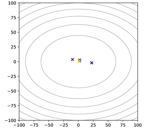
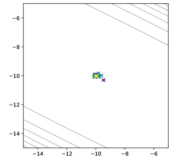
Figure 12: Results of the single optimization run using GA for the $2$-dimensional benchmark functions. The colored crosses indicate the spatial coordinates of the best individual at each generation. Black lines indicate the isolines of the functions.

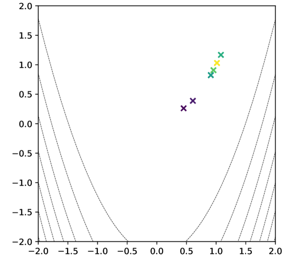
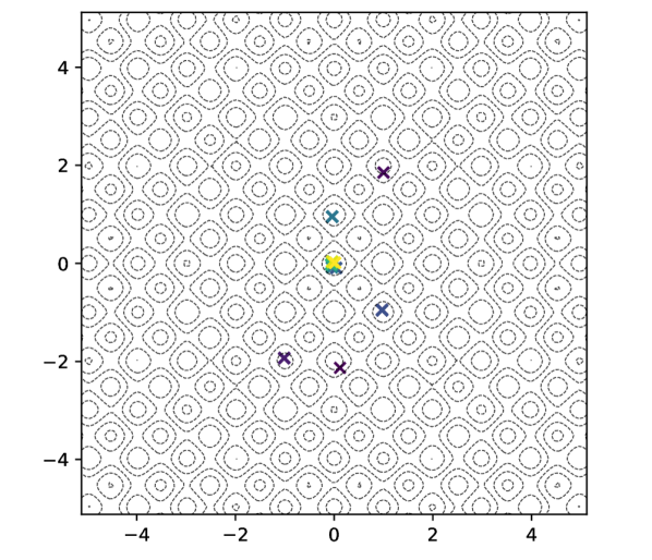
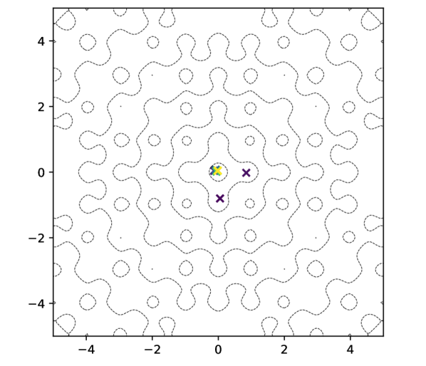
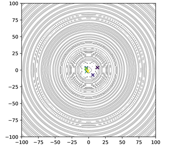
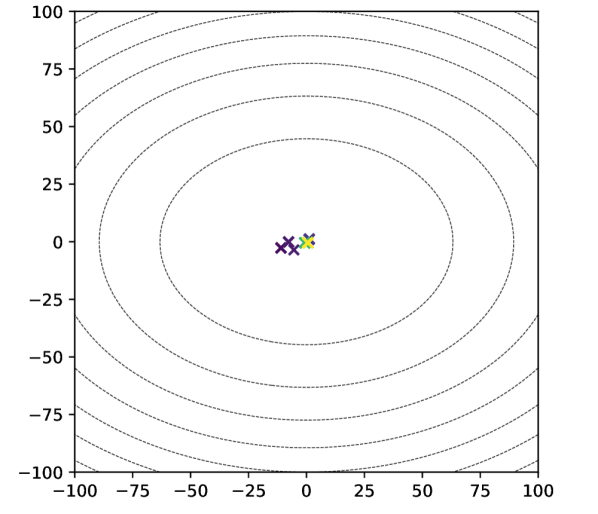
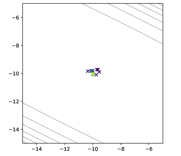
Figure 13: Results of the single optimization run using ASGA for the $2$-dimensional benchmark functions. The colored crosses indicate the spatial coordinates of the best individual at each generation. Black lines indicate the isolines of the functions.

We also measure the convergence as the Euclidean distance between the best individual fitness and the global optimum, and the spatial convergence as the Euclidean distance between the coordinates of the best individual and the coordinates of the optimal point. We kept the same numerical settings, only raising the number of generation to $1000$. Figure 14 presents the plots where we compare the trend using GA and ASGA: the proposed method shows a better performance, not only thanks to the faster convergence but also because in all the cases ASGA is able to get closer than the GA to the global optimum.

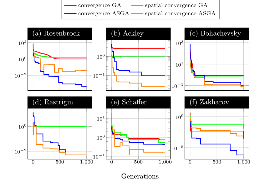
Figure 14: Convergence of GA and ASGA for the $2$-dimensional benchmark functions.

References

- [1] I. H. Abbott and A. E. Von Doenhoff. Theory of wing sections: including a summary of airfoil data. Courier Corporation, 2012.
- [2] E. P. Adorio and U. Diliman. Mvf-multivariate test functions library in C for unconstrained global optimization. Quezon City, Metro Manila, Philippines, pages 100–104, 2005.
- [3] M. M. Ali, C. Khompatraporn, and Z. B. Zabinsky. A numerical evaluation of several stochastic algorithms on selected continuous global optimization test problems. Journal of global optimization, 31(4):635–672, 2005.
- [4] T. Back. Evolutionary algorithms in theory and practice: evolution strategies, evolutionary programming, genetic algorithms. Oxford University Press, 1996.
- [5] J. Bect, D. Ginsbourger, L. Li, V. Picheny, and E. Vazquez. Sequential design of computer experiments for the estimation of a probability of failure. Statistics and Computing, 22(3):773–793, 2012.
- [6] C. J. Bélisle, H. E. Romeijn, and R. L. Smith. Hit-and-run algorithms for generating multivariate distributions. Mathematics of Operations Research, 18(2):255–266, 1993.
- [7] N. Botkin and V. Turova-Botkina. An algorithm for finding the chebyshev center of a convex polyhedron. Applied Mathematics and Optimization, 29(2):211–222, 1994.
- [8] R. A. Bridges, A. D. Gruber, C. R. Felder, M. Verma, and C. Hoff. Active Manifolds: A non-linear analogue to Active Subspaces. In Proceddings of the 36th International Conference on Machine Learning, ICML 2019, pages 764–772, Long Beach, California, USA, 9–15 June 2019.
- [9] M. D. Buhmann. Radial basis functions: theory and implementations, volume 12. Cambridge University Press, 2003.
- [10] C. Cartis and A. Otemissov. A dimensionality reduction technique for unconstrained global optimization of functions with low effective dimensionality. arXiv preprint arXiv:2003.09673, 2020.
- [11] R. Chelouah and P. Siarry. A continuous genetic algorithm designed for the global optimization of multimodal functions. Journal of Heuristics, 6(2):191–213, 2000.
- [12] K. M. Choromanski, A. Pacchiano, J. Parker-Holder, Y. Tang, and V. Sindhwani. From Complexity to Simplicity: Adaptive ES-Active Subspaces for Blackbox Optimization. In Advances in Neural Information Processing Systems, pages 10299–10309, 2019.
- [13] P. G. Constantine. Active subspaces: Emerging ideas for dimension reduction in parameter studies, volume 2 of SIAM Spotlights. SIAM, 2015.
- [14] P. G. Constantine, E. Dow, and Q. Wang. Active subspace methods in theory and practice: applications to kriging surfaces. SIAM Journal on Scientific Computing, 36(4):A1500–A1524, 2014.
- [15] P. G. Constantine, A. Eftekhari, and M. B. Wakin. Computing active subspaces efficiently with gradient sketching. In 2015 IEEE 6th International Workshop on Computational Advances in Multi-Sensor Adaptive Processing (CAMSAP), pages 353–356. IEEE, 2015.
- [16] C. Cui, K. Zhang, T. Daulbaev, J. Gusak, I. Oseledets, and Z. Zhang. Active Subspace of Neural Networks: Structural Analysis and Universal Attacks. arXiv preprint arXiv:1910.13025, 2019.
- [17] J. P. Cunningham and Z. Ghahramani. Linear dimensionality reduction: Survey, insights, and generalizations. The Journal of Machine Learning Research, 16(1):2859–2900, 2015.
- [18] N. Demo, M. Tezzele, A. Mola, and G. Rozza. Hull shape design optimization with parameter space and model reductions and self-learning mesh morphing. arXiv preprint arXiv:2101.03781, Submitted, 2021.
- [19] N. Demo, M. Tezzele, and G. Rozza. A non-intrusive approach for reconstruction of POD modal coefficients through active subspaces. Comptes Rendus Mécanique de l’Académie des Sciences, DataBEST 2019 Special Issue, 347(11):873–881, November 2019.
- [20] L. C. W. Dixon and G. P. Szego. The Global Optimization Problem: An Introduction. In Towards Global Optimisation, pages 1–15. North-Holland Pub. Co, Amsterdam, 1978.
- [21] Z. Drezner. A new genetic algorithm for the quadratic assignment problem. INFORMS Journal on Computing, 15(3):320–330, 2003.
- [22] T. A. El-Mihoub, A. A. Hopgood, L. Nolle, and A. Battersby. Hybrid genetic algorithms: A review. Engineering Letters, 13(2):124–137, 2006.
- [23] S. M. Elsayed, R. A. Sarker, and D. L. Essam. A new genetic algorithm for solving optimization problems. Engineering Applications of Artificial Intelligence, 27:57–69, 2014.
- [24] C. Emmeche. The garden in the machine: the emerging science of artificial life, volume 17. Princeton University Press, 1996.
- [25] L. J. Eshelman and J. D. Schaffer. Real-coded genetic algorithms and interval-schemata. In Foundations of genetic algorithms, volume 2, pages 187–202. Elsevier, 1993.
- [26] M. Guo and J. S. Hesthaven. Reduced order modeling for nonlinear structural analysis using Gaussian process regression. Computer Methods in Applied Mechanics and Engineering, 341:807–826, 2018.
- [27] R. M. Hicks and P. A. Henne. Wing design by numerical optimization. Journal of Aircraft, 15(7):407–412, 1978.
- [28] R. Hinterding. Gaussian mutation and self-adaption for numeric genetic algorithms. In Proceedings of 1995 IEEE International Conference on Evolutionary Computation, volume 1, page 384. IEEE, 1995.
- [29] J. H. Holland. Genetic algorithms and the optimal allocation of trials. SIAM Journal on Computing, 2(2):88–105, 1973.
- [30] J. H. Holland. Adaptation in natural and artificial systems: an introductory analysis with applications to biology, control, and artificial intelligence. MIT press, 1992.
- [31] M. Jamil and X.-S. Yang. A literature survey of benchmark functions for global optimisation problems. International Journal of Mathematical Modelling and Numerical Optimisation, 4(2):150–194, 2013.
- [32] M. Kumar, M. Husain, N. Upreti, and D. Gupta. Genetic algorithm: Review and application. Available at SSRN 3529843, 2010.
- [33] M. Laguna and R. Martí. Experimental testing of advanced scatter search designs for global optimization of multimodal functions. Journal of Global Optimization, 33(2):235–255, 2005.
- [34] L. Lovász and S. Vempala. Hit-and-run from a corner. SIAM Journal on Computing, 35(4):985–1005, 2006.
- [35] T. W. Lukaczyk, P. Constantine, F. Palacios, and J. J. Alonso. Active subspaces for shape optimization. In 10th AIAA multidisciplinary design optimization conference, page 1171, 2014.
- [36] H. Mühlenbein, M. Schomisch, and J. Born. The parallel genetic algorithm as function optimizer. Parallel computing, 17(6-7):619–632, 1991.
- [37] Y. Nesterov and V. Spokoiny. Random gradient-free minimization of convex functions. Foundations of Computational Mathematics, 17(2):527–566, 2017.
- [38] V. Picheny, T. Wagner, and D. Ginsbourger. A benchmark of kriging-based infill criteria for noisy optimization. Structural and Multidisciplinary Optimization, 48(3):607–626, 2013.
- [39] H. Qian, Y.-Q. Hu, and Y. Yu. Derivative-free optimization of high-dimensional non-convex functions by sequential random embeddings. In IJCAI, pages 1946–1952, 2016.
- [40] F. Romor, M. Tezzele, A. Lario, and G. Rozza. Kernel-based Active Subspaces with application to CFD parametric problems using Discontinuous Galerkin method. arXiv preprint arXiv:2008.12083, Submitted, 2020.
- [41] F. Romor, M. Tezzele, and G. Rozza. ATHENA: Advanced Techniques for High dimensional parameter spaces to Enhance Numerical Analysis. Submitted, 2020.
- [42] G. Rozza, M. Hess, G. Stabile, M. Tezzele, and F. Ballarin. Basic Ideas and Tools for Projection-Based Model Reduction of Parametric Partial Differential Equations. In P. Benner, S. Grivet-Talocia, A. Quarteroni, G. Rozza, W. H. A. Schilders, and L. M. Silveira, editors, Model Order Reduction, volume 2, chapter 1, pages 1–47. De Gruyter, Berlin, Boston, 2020.
- [43] M. L. Sanyang and A. Kabán. REMEDA: Random Embedding EDA for optimising functions with intrinsic dimension. In International Conference on Parallel Problem Solving from Nature, pages 859–868. Springer, 2016.
- [44] J. D. Schaffer, R. Caruana, L. J. Eshelman, and R. Das. A study of control parameters affecting online performance of genetic algorithms for function optimization. In Proceedings of the 3rd international conference on genetic algorithms, pages 51–60, 1989.
- [45] R. Sivaraj and T. Ravichandran. A review of selection methods in genetic algorithm. International journal of engineering science and technology, 3(5):3792–3797, 2011.
- [46] R. L. Smith. The hit-and-run sampler: a globally reaching markov chain sampler for generating arbitrary multivariate distributions. In Proceedings Winter Simulation Conference, pages 260–264. IEEE, 1996.
- [47] M. Tezzele, F. Ballarin, and G. Rozza. Combined parameter and model reduction of cardiovascular problems by means of active subspaces and POD-Galerkin methods. In D. Boffi, L. F. Pavarino, G. Rozza, S. Scacchi, and C. Vergara, editors, Mathematical and Numerical Modeling of the Cardiovascular System and Applications, volume 16 of SEMA-SIMAI Series, pages 185–207. Springer International Publishing, 2018.
- [48] M. Tezzele, N. Demo, M. Gadalla, A. Mola, and G. Rozza. Model order reduction by means of active subspaces and dynamic mode decomposition for parametric hull shape design hydrodynamics. In Technology and Science for the Ships of the Future: Proceedings of NAV 2018: 19th International Conference on Ship & Maritime Research, pages 569–576. IOS Press, 2018.
- [49] M. Tezzele, N. Demo, A. Mola, and G. Rozza. An integrated data-driven computational pipeline with model order reduction for industrial and applied mathematics. Special Volume ECMI, Springer, In Press, 2020.
- [50] M. Tezzele, N. Demo, and G. Rozza. Shape optimization through proper orthogonal decomposition with interpolation and dynamic mode decomposition enhanced by active subspaces. In R. Bensow and J. Ringsberg, editors, Proceedings of MARINE 2019: VIII International Conference on Computational Methods in Marine Engineering, pages 122–133, 2019.
- [51] M. Tezzele, N. Demo, G. Stabile, A. Mola, and G. Rozza. Enhancing CFD predictions in shape design problems by model and parameter space reduction. Advanced Modeling and Simulation in Engineering Sciences, 7(40), 2020.
- [52] M. Tezzele, F. Salmoiraghi, A. Mola, and G. Rozza. Dimension reduction in heterogeneous parametric spaces with application to naval engineering shape design problems. Advanced Modeling and Simulation in Engineering Sciences, 5(1):25, Sep 2018.
- [53] Z. Wang, F. Hutter, M. Zoghi, D. Matheson, and N. de Feitas. Bayesian optimization in a billion dimensions via random embeddings. Journal of Artificial Intelligence Research, 55:361–387, 2016.
- [54] O. Zahm, P. G. Constantine, C. Prieur, and Y. M. Marzouk. Gradient-based dimension reduction of multivariate vector-valued functions. SIAM Journal on Scientific Computing, 42(1):A534–A558, 2020.
- [55] G. Zhang, J. Zhang, and J. Hinkle. Learning nonlinear level sets for dimensionality reduction in function approximation. In Advances in Neural Information Processing Systems, pages 13199–13208, 2019.