Expectation-Maximization Algorithm for Identification of Mesh-based Compartment Thermal Model of Power Modules

Abstract

Accurate knowledge of temperatures in power semiconductor modules is crucial for proper thermal management of such devices. Precise prediction of temperatures allows to operate the system at the physical limit of the device avoiding undesirable over-temperatures and thus improve reliability of the module.

Commonly used thermal models can be based on detailed expert knowledge of the device’s physical structure or on precise and complete temperature distribution measurements. The latter approach is more often used in the industry. Recently, we have proposed a linear time invariant state-space thermal model based on a compartment representation and its identification procedure that is based on the Expectation-Maximization algorithm from incomplete temperature data. However, the model still requires to measure temperatures of all active elements.

In this contribution, we aim to relax the need for all measurements. Therefore, we replace the previous dark gray-box approach with a structured compartment model. The structure of the model is designed by a mesh-based discretization of the physical layout of the module. All compartments are assumed to share parameters that are identified from the data of the measured elements. Temperatures of the unmeasured elements are predicted using the shared parameters.

Identification of the parameters is possible only with suitable regularization due to limited amount of the data. In particular, the model tightening is accomplished by sharing parameters among compartments and by constraining the process covariance matrix of the model in this contribution. Applicability of the proposed identification procedure is discussed in terms of growing state-space and therefore speeding up of the identification algorithm is suggested. Performance of the proposed approach is tested and demonstrated on simulated data.

Keywords: expectation-maximization, state space model, thermal model, compartment model, identification, power electronics, mesh-based, covariance matrix, regularization

1 Introduction

Monitoring of temperature distribution and its accurate prediction in power semiconductor modules is fundamental for the proper thermal management, that enables to operate system at the physical limit and prevents device failures due to undesirable thermal stresses. Therefore, the integration of the precise thermal model into the thermal protection algorithm is essential, since the direct measurement of all temperature distribution is very often infeasible (e.g. due to necessity for device capsuling or low cost production claims).

A popular class of models used for heat transfer simulations are models based on numerical discretization such as Finite Difference Method (FDM), Finite Element Method (FEM) or Finite Volume Method (FVM). These methods yield very accurate results but at the expense of high computational requirements and thus they cannot be used in online prediction. Moreover, the design and especially validation of these models can be very time-consuming and without precise knowledge of device’s physical structure difficultly realizable.

Another class of models is based on Lumped Parameter Thermal Networks (LPTNs) using thermal resistors and thermal capacitors as an analoqy to electrical circuits for modeling of the heat transfer in the devices. Generally, LPTNs produce reasonably accurate results requiring much less computational time in comparison to models based on numerical discretization methods. LPTNs can be classified as dark gray-box, light gray-box or white-box models depending on the number of used equivalent Resistor and Capacitor (RC) elements [1]. Dark gray-box LPTNs use only units of elements and therefore computational requirements of such models can be very low. On the contrary dark gray-box LPTNs are strongly abstracted, the information about temperature distribution in the device is not complete (only selected points in the device can be monitored) and several thermal phenomena (e.g. coupling effect or temperature distribution in the segment like a chip) are ignored.

Increasing microcontrollers computational performance enables to employ improved LPTNs with more complicated structure (light gray-box or white-box models). Using higher level of elements in the LPTN can lead to improved solution accuracy [2] and finer details, e.g. spatial temperature distribution, boundary conditions or coupling effect [3, 4] can be covered in the model. Nevertheless, RC parameters of such models are very often extracted from the complicatedly calibrated FEM model using transient (step) response analysis and following exponential fitting techniques applied on transient thermal impedance curves. An interesting approach how to create light gray- or white-box RC model is to uses a mesh-based LPTN [5, 6], that can be identify from a geometric and material description of the device. This standard identification procedure is strongly dependent on quality of information about device physical structure and still requires rich experience to obtain reasonable results [2].

Recently, authors of this contribution proposed the Linear Time Invariant (LTI) State Space (SS) compartment thermal model and its self-tuning identification using Expectation-Maximization (EM) algorithm in [7]. This approach enables identification of the model from incomplete temperature data and allows to combine sets of various measurements of Temperature Sensitive Electrical Parameters (TSEPs) or direct measurements. However, the model still requires to measure temperatures of all active elements. In this paper, we aim to relax the need for all measurements. Therefore we investigate the mesh-based structured compartment model in this paper. In the sense of classification into the black-/gray-/white-box model, [7] can be seen as dark gray-box model. The proposed mesh-based model falls into white-box models, since there is much finer compartment structure based on discretization of the physical layout of the module. This results in a growing state space of temperatures and growing dimension of the state matrix in the proposed LTI SS model. For that reason, the model is tightened by sharing parameters, that are identified from the data. The possibility to apply Expectation-Maximization algorithm for the identification of the consequently growing LTI SS is studied in detail.

2 Mesh-based compartment structure

The proposed LTI SS thermal model is based on a compartment representation of the studied power semiconductor module. The compartment model may be understood as a coarsely discretized model in the sense of numerical methods. In other words, each compartment stands for a relatively spacious control volume of the area of interest. In comparison to the numerical discretization, the module is possible to be represented by only units of compartments, although a finer compartment representation can give better results. For that reason, the models based on mesh representation and comprising structured compartments (circa hundreds of compartments what is still much less than it is usual in numerical models) are objects of our interest.

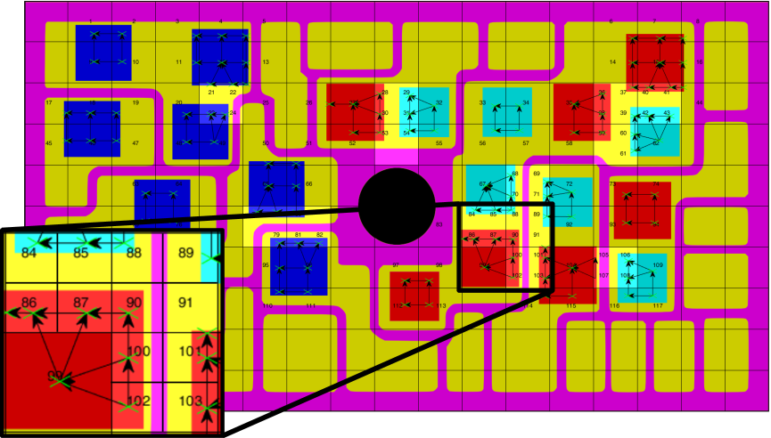
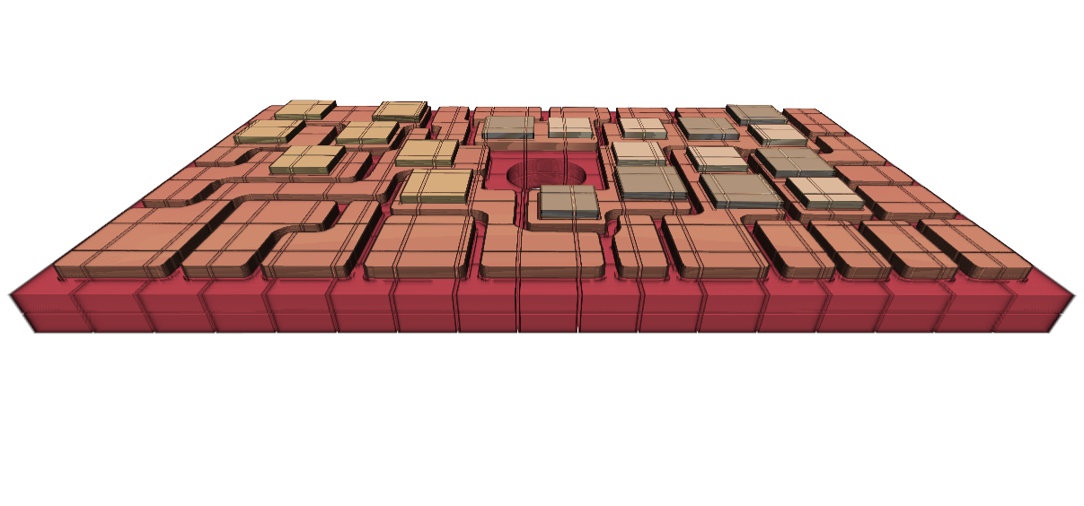
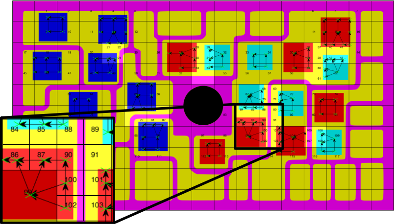
The three-dimensional volume of entire domain of the investigated power module is discretized into rectangular elements (cubes or cuboids) in a uniform Cartesian grid. To these elements we refer as to compartments. Each basic-sized compartment can be further refined into four finer compartments in X- and Y-axis in quadtree sense in the case that the compartment contains more various components (e.g. a part of diode’s volume and a part of transistor’s volume are located in the same compartment).

(a) Scheme of the layer arrangement

(b) Complicated layout comprising diodes and transistors

Figure 1: Semikron power electronics module SK20 DGDL 065 ET

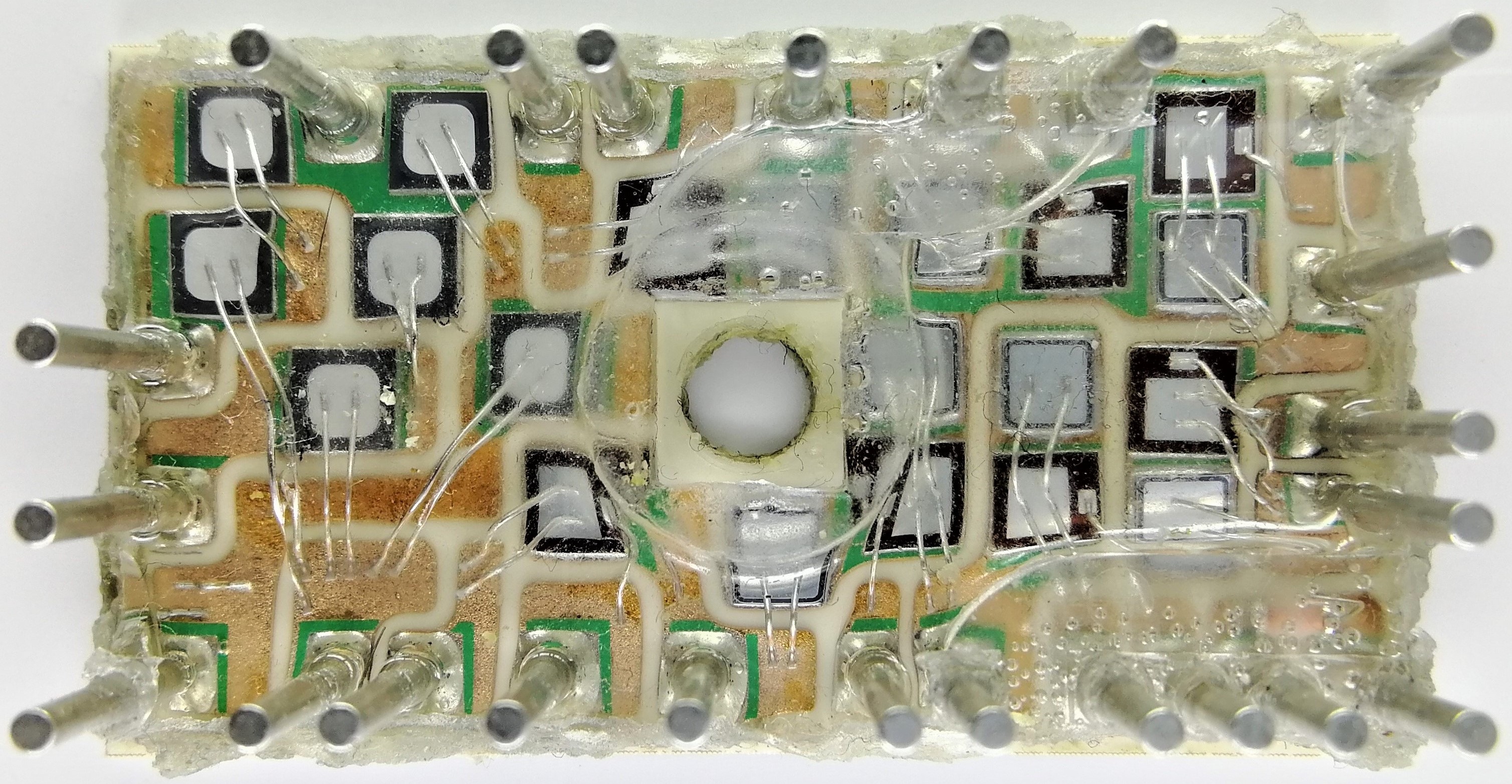
A selection of the basic discretization level is a trade-off between growing number of compartments and a quality of the model. A layer arrangement in one axis (Z-axis in our case) is typical for a common power semiconductor module (Figure 1a), whereas more complicated layout comprising diodes or transistors covers the surface (Figure 1b) in remaining two axes (X- and Y-axis). For this reason, the suggested design of the discretization divides into the selection of the number of compartment’s layers and selection of the fineness of the power module surface grid.

The specific discretization levels used in this paper for testing the proposed identification method are discussed in Section 5.

3 Compartment state space model

The governing equation for the LTI SS model is the well known heat transfer equation

$$\text{div}\left(\lambda\text{grad}T\right)+p=\rho c_{\mathrm{p}}\frac{\partial T}{\partial t},$$ (1)

where $T$ stands the temperature, $p$ is the internal heat source (with base units $[\mathrm{W/m^{3}}]$), $\lambda$ is the thermal conductivity coefficient, $\rho$ is the density of the material, and $c_{\mathrm{p}}$ is the specific heat capacity at constant pressure. Under the assumption of uniform constant thermal properties of compartments, equation (1) can be discretized [8] using fully explicit scheme into the form

$$T_{i,t+1}=T_{i,t}+\Delta\tau\left(\sum_{j\in\mathcal{S}_{i}}k_{i,j}(T_{j,t}-T_{i,t})+z_{i}P_{i,t}\right),$$ (2)

where $T_{i,t}$ and $P_{i,t}$ are the temperature and the internal volumetric heat source inside the compartment $i$ in the discrete time $t$, $t\in\mathbb{Z}$. The time step is denoted by $\text{$\Delta$}\tau$ and $\mathcal{S}_{i}$ is the set of indexes of the compartments adjacent to the $i$th compartment such that we assume thermal coupling with the $i$th compartment. More detail can be seen in [7].

The proposed compartment model (2) can be viewed as a particular case of directed graphs. Using graph theory [9], the heat transfer between compartments given by equation (2) may be described by a directed graph with vertices $T_{i}$ and directed edges $k_{i,j}$. Coefficients $k_{i,j}$ can be arbitrarily sorted into a vector $\boldsymbol{k}\text{$\in$}\mathbb{R}^{m}$, which corresponds to the ordering of edges in the graph. Then the directed graph can be represented by an incidence matrix $\mathcal{J}$. The incidence matrix is a sparse matrix of size $n\text{$\times$}m$ in general, where $n$ is the number of vertices (i.e. compartments) and $m$ is the number of edges (i.e. valid coefficients $k_{i,j}$). The element $j_{i,l}$ of the incidence matrix $\mathcal{J}$ is defined by the relation

$$j_{i,l}=\left\{\begin{array}[]{ll}1&\textrm{\qquad if }T_{i}\textrm{ is the tail of the }l\textrm{-th edge}\\ -1&\textrm{\qquad if }T_{i}\textrm{ is the head of the }l\textrm{-th edge}\\ 0&\textrm{\qquad otherwise}.\end{array}\right.$$ (3)

Introducing a temperature vector $\boldsymbol{T}_{t}=[T_{1,t},\ldots,T_{n,t}]^{\prime}$, a vector of volumetric power sources (power losses) $\boldsymbol{P}_{t}=[P_{1,t},\ldots,P_{n,t}]^{\prime}$ and a parameter vector $\boldsymbol{z}=[z_{1},\ldots,z_{n}]^{\prime}$, and employing the incidence matrix $\mathcal{J}$ and the parameter vector $\boldsymbol{k}$, discrete thermal dynamic equation (2) can be written in the form using the parametrization by $\boldsymbol{k}$ and $\boldsymbol{z}$

$$\boldsymbol{T}_{t+1} = \boldsymbol{T}_{t}-\Delta\tau\mathcal{I}\mathrm{\text{diag}(\mathcal{C}\boldsymbol{k})\mathcal{J}^{\prime}}\boldsymbol{T}_{t}+\Delta\tau\mathcal{B}\mathrm{\text{diag}}(\mathcal{A}\boldsymbol{z})\boldsymbol{P}_{t}$$ (4)

$$= \boldsymbol{T}_{t}-\Delta\tau\mathcal{I}\text{diag}(\mathcal{J}^{\prime}\boldsymbol{T}_{t})\mathcal{C}\boldsymbol{k}+\Delta\tau\mathcal{B}\text{diag}(\boldsymbol{P}_{t})\mathcal{A}\boldsymbol{z},$$ (5)

where matrix $\mathcal{I}$ is a matrix obtained from incidence matrix $\mathcal{J}$ by replacement $1\rightarrow 0$. Matrices and $\mathcal{A},\mathcal{B}$ and $\mathcal{C}$ in equations (4) and (5) are auxiliary matrices of elementary vectors. If $\text{$\mathcal{A}$}=I_{n}$, $\text{$\mathcal{B}$}=I_{n}$, $\text{$\mathcal{C}$}=I_{m}$, where $I_{n}$ is the identity matrix $n\text{$\times$}n$, we get exactly the same set of equations as in (2).

In many cases, the power losses $\boldsymbol{P}_{t}$ could be considered only for particular compartments (e.g. for compartments corresponding to transistors or diodes in the case of power module modeling). Furthermore we wish to have the mesh-based compartment model described by shared parameters. It means that selected sets of coefficients $k_{i,j}$ and $z_{i}$ are required to be identical. These presumptions are very desirable for the following identification procedure, since the dimension of temperature vector in the proposed mesh-based model is relatively high.

In general, vectors $\boldsymbol{z}=[z_{1},\ldots,z_{n_{z}}]^{\prime}$, $\boldsymbol{P}_{t}=[P_{1,t},\ldots,P_{n_{P},t}]^{\prime}$, and $\boldsymbol{k}=[k_{1},\ldots,k_{n_{k}}]^{\prime}$ are of arbitrary lengths $n_{z}$, $n_{P}$, and $n_{k}$ respectively. Then $\mathcal{A}$ is a matrix $n_{P}\text{$\times$}n_{z}$ of scaled elementary row vectors mapping vector $\boldsymbol{z}$ to the corresponding heat sources, $\mathcal{B}$ is a matrix $n\text{$\times$}n_{P}$ of scaled elementary row vectors mapping heat sources to the corresponding compartments, and $\mathcal{C}$ is a matrix $m\text{$\times$}n_{k}$ of scaled elementary row vectors mapping vector $\boldsymbol{k}$ to the corresponding edges of the graph representation (i.e. mapping vector $\boldsymbol{k}$ to the corresponding differences $T_{j,t}-T_{i,t}$). The scale of each elementary vector corresponds to a certain weight of transfer coefficients among compartments in the case that only a fraction of compartment volume is occupied by the studied device, or in the case that compartment refining is utilized during designing of the mesh-based model. Then, these weights are dependent on the different volumes and outer surfaces of base-size compartments and refined compartments. In other cases the default scale is set to one.

Further, equations (4)–(5) can be rewritten in a more pleasant form. Establishing matrices $A$, $B$ and $M$

$$A = I_{n}-\Delta\tau\mathcal{I}\mathrm{\text{diag}(\mathcal{C}\boldsymbol{k})\mathcal{J}^{\prime}},$$ (6)

$$B = \Delta\tau\mathcal{B}\mathrm{\text{diag}}(\mathcal{A}\boldsymbol{z}),$$ (7)

$$M_{t} = \left[-\mathcal{I}\text{diag}(\mathcal{J}^{\prime}\boldsymbol{T}_{t})\mathcal{C},\,\text{$\mathcal{B}$diag}(\boldsymbol{P}_{t})\mathcal{A}\right]$$ (8)

and assuming an additional zero-mean Gaussian noise $\boldsymbol{w}_{t}\text{$\in\ $}\mathbb{R}^{n}$ with a covariance matrix $Q$, $\boldsymbol{w}_{t}\sim\mathcal{N}\left(\boldsymbol{w}_{t}|\boldsymbol{0},Q\right)$, equation (4) can be put into the standard form of the explicit discrete LTI state equation

$$\boldsymbol{T}_{t+1} = A\boldsymbol{T}_{t}+B\boldsymbol{P}_{t}+\boldsymbol{w}_{t}$$ (9)

$$= \boldsymbol{T}_{t}+\Delta\tau M_{t}\boldsymbol{\theta}+\boldsymbol{w}_{t},$$ (10)

$$\text{$\hphantom{\boldsymbol{\boldsymbol{}_{t+1}}}$}\boldsymbol{\theta} = \left[\boldsymbol{k}^{\prime},\boldsymbol{z}^{\prime}\right]^{\prime}.$$ (11)

with the state vector $\boldsymbol{T}_{\bullet}$ and the input vector $\boldsymbol{P}_{\bullet}$. Equation (10) is a notation enabling to use a least squares method for estimating unknown parameter vectors $\boldsymbol{k}$ and $\boldsymbol{z}$ of the proposed model.

For completeness of the model, we define the vector of measured temperatures as $\boldsymbol{y}_{t}$ and observation model (output equation)

$$\boldsymbol{y}_{t}=C\boldsymbol{T}_{t}+\boldsymbol{v}_{t},$$ (12)

where $C\in\mathbb{R}^{n_{y}\times n}$ is the matrix comprising elementary row vectors corresponding to the indices of $n_{y}$ measured (observed) compartment temperatures, and $\boldsymbol{v}_{t}$ is a zero-mean Gaussian noise with a covariance matrix $R$, $\boldsymbol{v}_{t}\sim\mathcal{N}\left(\boldsymbol{v}_{t}|\boldsymbol{0};R\right).$ The length of the measurement vector is denoted by $N,$ $t\in 1:N.$ Then, equations (9) and (12) form a standard discrete LTI SS model with unknown parameters $\boldsymbol{\theta}$.

4 Expectation-maximization algorithm

The Expectation-Maximization (EM) algorithm [10] is a standard technique that allows to estimate model parameters from data sets with missing or hidden variables. Its application for the identification of the proposed model (9)–(12) is now reviewed.

The objective of EM algorithm is to maximize the log likelihood of the measured data

$$\log p\left(Y|P,\boldsymbol{\theta}\right)=\log\int\limits_{T}p\left(T,Y|P,\boldsymbol{\theta}\right)dT,$$ (13)

where $T=\left\{\boldsymbol{T}_{1},\cdots,\boldsymbol{T}_{N}\right\}$, $P=\left\{\boldsymbol{P}_{1},\cdots,\boldsymbol{P}_{N}\right\}$, $Y=\left\{\boldsymbol{y}_{1},\cdots,\boldsymbol{y}_{N}\right\}$. In essence, the algorithm is proposed to approximate the correct marginal likelihood approach by iterative maximization of its lower bound. The lower bound $\mathcal{F}\left(\mathcal{Q},\boldsymbol{\theta}\right)$ is derived [11] using any distribution $\Phi\left(T\right)$ as

$$\log\int\limits_{T}p\left(T,Y|P,\boldsymbol{\theta}\right)dT=\log\int\limits_{T}\Phi\left(T\right)\frac{p\left(T,Y|P,\boldsymbol{\theta}\right)}{\Phi\left(T\right)}dT=\hskip 56.9055pt$$

$$\hskip 28.45274pt=\log E_{\Phi\left(T\right)}\left[\frac{p\left(T,Y|P,\boldsymbol{\theta}\right)}{\Phi\left(T\right)}\right]\geq E_{\Phi\left(T\right)}\left[\log\frac{p\left(T,Y|P,\boldsymbol{\theta}\right)}{\Phi\left(T\right)}\right]=\hskip 28.45274pt$$ (14)

$$\vphantom{\int\limits_{X}}\hskip 56.9055pt=E_{\Phi\left(T\right)}\left[\log p\left(T,Y|P,\boldsymbol{\theta}\right)\right]-E_{\Phi\left(T\right)}\left[\log\Phi\left(T\right)\right]=\mathcal{F}\left(\Phi,\boldsymbol{\theta}\right).$$

To find the maximum likelihood (ML) estimate of unknown parameters $\boldsymbol{\theta}$, the EM algorithm seeks to maximize the lower bound $\mathcal{F}\left(\Phi,\boldsymbol{\theta}\right)$ of the observed data marginal likelihood (13) by alternating so called Expectation step (E-step) and Maximization step (M-step). With the aim to identify the proposed LTI SS model, we discuss these steps in the following text in more detail.

4.1 Expectation step – Rauch Tung Striebel Smoother

In the $r$-th E-step, the lower bound $\mathcal{F}(\Phi,\boldsymbol{\theta}^{r-1})$ is maximized with respect to the distribution $\Phi$ holding fixed parameter vector $\boldsymbol{\theta}^{r-1}$. Assuming that we have some parameter values $\boldsymbol{\theta}^{r-1}$ available from the previous M-step, it is possible to show, that the desired distribution $\Phi^{r}\left(T\right)$ is exactly the conditional distribution of $T$ [11]

$$\Phi^{r}\left(T\right)=p\left(T|Y,P,\boldsymbol{\theta}^{r-1}\right)$$ (15)

Since for the known values of the parameter vector $\boldsymbol{\theta}^{r-1}$, i.e. for known values of matrix $A$ and $B$ given by (6) and (7), the system (9),(12) forms a state space model, the full distribution of all temperatures (15) can be determined by Rauch Tung Striebel Smoother (RTSS) [12]. The RTSS is a two-pass algorithm (Algorithm 1) for fixed interval smoothing, where the first pass is the regular forward Kalman filter and the second pass is the backward smoother.

The output of the RTSS is the smoothed posterior Gaussian distribution $p(\boldsymbol{T}_{t}|P,\boldsymbol{\theta}^{r-1},Q^{r-1},R)$. Moreover theRTSS purveys the smoothed posterior joint distribution

$$p\left(\left[\begin{array}[]{c}\boldsymbol{T}_{t+1}\\ \boldsymbol{T}_{t}\end{array}\right]|P,\boldsymbol{\theta}^{r-1},Q^{r-1},R\right)=\mathcal{N}\left(\left[\begin{array}[]{c}\boldsymbol{T}_{t+1}\\ \boldsymbol{T}_{t}\end{array}\right]|\left[\begin{array}[]{c}\boldsymbol{x}_{t+1}^{N}\\ \boldsymbol{x}_{t}^{N}\end{array}\right],\left[\begin{array}[]{cc}V_{t+1}^{N}&V_{t+1,t}^{N}\\ \left(V_{t+1,t}^{N}\right)^{\prime}&V_{t}^{N}\end{array}\right]\right),$$ (16)

where the notation from the Algorithm 1 is used. Note that the temperature random variable is marked by $\boldsymbol{T}_{\bullet}$, whereas the smoothed estimate (or the expected value in other words) by $\boldsymbol{x}_{\bullet}^{N}$.

As can be seen, the posterior distributions determined by RTSS are also conditioned by covariance matrices $Q^{r-1}$ and $R$. These matrices can be either known in many cases and fixed by user or they can be added into the identification process. In this paper, we assume covariance matrix $R$ of measurement noise to be known and we incorporate the identification of process noise covariance matrix $Q$ into the estimation procedure. Therefore, $Q^{r-1}$ is available in the $r$-th E-step similarly to parameters vector $\boldsymbol{\theta}^{r-1}$. The estimation of $Q^{r-1}$ is the objective of the previous maximization step discussed in subsection 4.3.

4.2 Speeding up of E-step using steady-state covariances

The time and memory burdens of RTSS directly depend on the dimension of state space vector $\boldsymbol{T}_{t}$ (we assume the dimension of vector $\boldsymbol{T}_{t}$ much larger than dimensions of vectors $\boldsymbol{P}_{t}$ and $\boldsymbol{y}_{t}$) and on the number of measurements $N$. Since we are using the model with hundreds or even thousands of compartments (corresponding to the dimension of $\boldsymbol{T}_{t}$ and each dimension of covariance matrices $V_{t+1}^{\text{$\bullet$}}$), especially the inversion $(V_{t+1}^{t})^{-1}$(line 10 in Algorithm 1) in each for-cycle iteration of the backward pass is very time consuming apart from a large matrix multiplication in the remaining parts of RTSS. Besides, storing covariance matrices $V_{t}^{t}$ and $V_{t+1}^{t}$ in the forward pass (necessary for backward pass) is strongly memory-consuming as the number of observation $N$ increases.
1:  input $A,$ $B,$ $C,$ $Q,$ $R,$          $\boldsymbol{x}_{1}^{1}=\boldsymbol{T}_{1},$ $\boldsymbol{P}_{t},$ $\boldsymbol{y}_{t}$, $N$  $V_{S}^{-}$:  $\left(CV_{S}^{-}C^{\prime}+R\right)^{-1}$ 2:  for $t=1:1:N-1$ 3:   $\boldsymbol{x}_{t+1}^{t}=A\mathbf{x}_{t}^{t}+B\boldsymbol{P}_{t}$ 4:   $V_{t+1}^{t}=AV_{t}^{t}A^{\prime}+Q$ 5:   $K_{t+1}=V_{t+1}^{t}C^{\prime}(CV_{t+1}^{t}C^{\prime}+R)^{-1}$ 6:   $V_{t+1}^{t+1}=V_{t+1}^{t}-K_{t+1}CV_{t+1}^{t}$ 7:   $\boldsymbol{x}_{t+1}^{t+1}=\boldsymbol{x}_{t+1}^{t}+K_{t+1}(\boldsymbol{y}_{t+1}-C\boldsymbol{x}_{t+1}^{t})$ 8:  end for  $V_{S}^{N}:$ 9:  for $t=N-1:-1:1$ 10:   $J_{t}=V_{t}^{t}A^{\prime}(V_{t+1}^{t})^{-1}$ 11:   $V_{t}^{N}=V_{t}^{t}+J_{t}(V_{t+1}^{N}-V_{t+1}^{t})J_{t}^{\prime}$ 12:   $V_{t+1,t}^{N}=V_{t+1}^{N}J_{t}^{\prime}$ 13:   $\boldsymbol{x}_{t}^{N}=\boldsymbol{x}_{t}^{t}+J_{t}(\boldsymbol{x}_{t+1}^{N}-A\boldsymbol{x}_{t}^{t}-B\boldsymbol{P}_{t})$ 14:  end for Algorithm 1 original RTSS     1:  input $A,$ $B,$ $C,$ $Q,$ $R,$          $\boldsymbol{x}_{1}^{1}=\boldsymbol{T}_{1},$ $\boldsymbol{P}_{t},$ $\boldsymbol{y}_{t}$, $N$ 2:  compute Riccati equation for $V_{S}^{-}$: $V_{S}^{-}=AV_{S}A^{\prime}-AV_{S}^{-}C^{\prime}\left(CV_{S}^{-}C^{\prime}+R\right)^{-1}CV_{S}^{-}A^{\prime}+Q$ 3:  $K_{S}=V_{S}^{-}C^{\prime}\left(CV_{S}^{-}C^{\prime}+R\right)^{-1}$ 4:  $V_{S}^{+}=\left(I_{n}-K_{S}C\right)V_{S}^{-}$ 5:  for $t=1:1:N-1$ 6:   $\boldsymbol{x}_{t+1}^{t}=A\mathbf{x}_{t}^{t}+B\boldsymbol{P}_{t}$ 7:   $\boldsymbol{x}_{t+1}^{t+1}=\boldsymbol{x}_{t+1}^{t}+K_{S}(\boldsymbol{y}_{t+1}-C\boldsymbol{x}_{t+1}^{t})$ 8:  end for   9:  $J_{S}=V_{S}^{+}A^{\prime}(V_{S}^{-})^{-1}$ 10:  compute Lyapunov equation for $V_{S}^{N}:$ $V_{S}^{N}=J_{S}V_{S}^{N}J_{S}^{\prime}+\left(V_{S}^{+}-J_{S}V_{S}^{-}J_{S}^{\prime}\right)$ 11:  for $t=N-1:-1:1$ 12:   $\boldsymbol{x}_{t}^{N}=\boldsymbol{x}_{t}^{t}+J_{S}(\boldsymbol{x}_{t+1}^{N}-A\boldsymbol{x}_{t}^{t}-B\boldsymbol{P}_{t})$ 13:  end for Algorithm 2 RTSS with steady covariances

For these reasons, we suggest to use steady covariance matrices in the RTSS which significantly reduces the computational requirements [13]. The implementation of the RTSS with steady covariances is shown in Algorithm 2.

Riccati equation on line 2 and Lyapunov equation on line 10 of Algorithm 2 can be evaluated by direct method or solvers (e.g. idare and dlyap Matlab’s in-build function) or iteratively using e.g. Newton techniques. Specifically in our case, we employed Modified Newton method for discrete-time algebraic Riccati equations [14] and Matlab’s function dlyap for solving discrete-time Lyapunov equations.

For an effective implementation, it is sufficient to collect only few statistics of relatively small size (square of the number of compartments) for the following M-step. The necessary statistics utilized in the M-step and obtained from RTSS using steady covariance matrices are

$$XX^{\prime}\equiv(N-1)V_{S}^{N}+\sum_{t=1}^{N-1}\boldsymbol{x}_{t}^{N}\left(\boldsymbol{x}_{t}^{N}\right)^{\prime} XU^{\prime}\equiv\sum_{t=1}^{N-1}\boldsymbol{x}_{t}^{N}\boldsymbol{P}_{t}^{\prime}$$

$$ZZ^{\prime}\equiv(N-1)V_{S}^{N}+\sum_{t=1}^{N-1}\boldsymbol{x}_{t+1}^{N}\left(\boldsymbol{x}_{t+1}^{N}\right)^{\prime} ZU^{\prime}\equiv\sum_{t=1}^{N-1}\boldsymbol{x}_{t+1}^{N}\boldsymbol{P}_{t}^{\prime}$$ (17)

$$XZ^{\prime}\equiv(N-1)J_{S}\left(V_{S}^{N}\right)^{\prime}+\sum_{t=1}^{N-1}\boldsymbol{x}_{t}^{N}\left(\boldsymbol{x}_{t+1}^{N}\right)^{\prime} UU^{\prime}\equiv\sum_{t=1}^{N-1}\boldsymbol{P}_{t}\boldsymbol{P}_{t}^{\prime}$$

For comparison, the form of statistics derived by the original full RTSS (Algorithm 1) and utilizable for the M-step can be found in [7].

4.3 Maximization step – Maximum Likelihood Estimate

In the $r$-th M-step, the lower bound $\mathcal{F}(\Phi^{r},\boldsymbol{\theta})$ is maximized with respect to the unknown model parameters $\boldsymbol{\theta}$ and noise covariance matrix $Q$ holding distribution $\Phi^{r}(T)$ fixed. The distribution $\Phi^{r}(T)$ is the smoothed posterior distribution (16) evaluated in the previous E-step of EM algorithm. Then, the new updates of parameters $\boldsymbol{\theta}^{r}$ and noise covariance matrix $Q^{r}$are given by

$$\boldsymbol{\theta}^{r},Q^{r}\text{=} \arg\max_{\boldsymbol{\theta},Q}\sum\limits_{1}^{N-1}E_{\Phi^{r}(T)} \Bigl{\{}\ln|Q^{-1}||R^{-1}|-\left(\Delta\boldsymbol{T}_{t}-M_{t}\boldsymbol{\theta}\right)^{\prime}Q^{-1}\left(\Delta\boldsymbol{T}_{t}-M_{t}\boldsymbol{\theta}\right)+$$ (18)

$$\vphantom{\ln|Q^{-1}||R^{-1}|-\left(\Delta\boldsymbol{T}_{t}-M_{t}\boldsymbol{\theta}\right)^{\prime}Q^{-1}\left(\Delta\boldsymbol{T}_{t}-M_{t}\boldsymbol{\theta}\right)}-\text{ $\left(\boldsymbol{y}_{t}-C\boldsymbol{T}_{t}\right)^{\prime}$}R^{-1}\text{ $\left(\boldsymbol{y}_{t}-C\boldsymbol{T}_{t}\right)$}\Bigr{\}}$$

where $\Delta\boldsymbol{T}_{t}=\Delta\tau^{-1}(\boldsymbol{T}_{t+1}-\boldsymbol{T}_{t})$, $E_{\Phi^{r}(T)}(\cdot)$ stands for the expectation value with respect to the distribution (16) and $|\cdot|$ denotes the determinant of the particular matrix.

It is easy to show, that the ML estimator of (18) is of the form

$$\boldsymbol{\theta}^{r}=\left(\sum_{t=1}^{N-1}E_{\Phi^{r}(T)}\left\{M_{t}^{\prime}\left(Q^{r}\right)^{-1}M_{t}\right\}\right)^{-1}\sum_{t=1}^{N-1}E_{\Phi^{r}(T)}\left\{M_{t}^{\prime}\left(Q^{r}\right)^{-1}\Delta\boldsymbol{T}_{t}\right\}$$ (19)

$$Q_{\textrm{full}}^{r}\text{=}\frac{1}{N-1}\sum\limits_{t=1}^{N-1}E_{\Phi^{r}(T)}\Bigl{\{}\Delta\boldsymbol{T}_{t}\Delta\boldsymbol{T}_{t}^{\prime}-\Delta\boldsymbol{T}_{t}\left(M_{t}\boldsymbol{\theta}^{r}\right)^{\prime}-M_{t}\boldsymbol{\theta}^{r}\left(\Delta\boldsymbol{T}_{t}\right)^{\prime}+M_{t}\boldsymbol{\theta}^{r}\left(M_{t}\boldsymbol{\theta}^{r}\right)^{\prime}\Bigr{\}}$$ (20)

where the individual expected terms can be expressed using only statistics (17) obtained by RTSS in the previous $r$-th E-step. These terms are given in A in the detail.

The computational problem lies in the mutual cross dependency of $\boldsymbol{\theta}^{r}$ on $Q^{r}$ and vice versa. This obstacle is connected with the structure of desired covariance matrix $Q$ and may vanish in some particular case. Moreover, the number of elements in the covariance matrix $Q$ is much higher than dimension of parameters vector $\boldsymbol{\theta}$ and thus a regularization of the problem (a shrinkage of covariance matrix estimation) is greatly desirable. Therefore, we investigate carefully the structure of the covariance matrix $Q$ now and discuss possible solutions.

4.4 Structure of process noise covariance matrix

1. An easy approach is to assume the covariance matrix $Q$ in the diagonal form with a constant on the diagonal, $Q\overset{!}{=}qI_{n}$. In such case, equation (19) can be simplified, since the term $\left(qI_{n}\right)^{-1}$ is possible to completely eliminate from the expression for $\boldsymbol{\theta}^{r}$ (19). Thus the evaluation of $\boldsymbol{\theta}^{r}$ is not dependent on the constrained covariance matrix $Q$ and can be directly executed. The formulation of M-step is then similar to ordinary least squares method but with proper considering of expected values. The formula for computation of the covariance matrix $q^{r}I_{n}$, or scalar value $q^{r}$ actually, reads

   $$q^{r}=\frac{1}{n}\Tr\left(Q_{\textrm{full}}^{r}\right).$$ (21)

   This case together with specific form of equations (19) and (20) is described by authors in [7].

2. There exist several other constraints on the covariance matrix $Q$, where direct derivation of the estimator is feasible. One representative of this group is non-homogeneous diagonal covariance matrix (compare with weighted least squares method), $Q\overset{!}{=}\text{diag}\left(\boldsymbol{q}\right)$, where $\boldsymbol{q}=[q_{1},\ldots,q_{n}]^{\prime}$. In such case, the form of ML estimators of $\boldsymbol{\theta}^{r}$ and $Q_{\textrm{diag}}^{r}$ remain as in (19) and (20), only with consideration that non-diagonal elements of $Q^{r}$ are zeros,

   $$\boldsymbol{q}^{r}\text{=}\text{diag}\left(Q_{\textrm{full}}^{r}\right).$$ (22)

   The mutual cross dependency of $\boldsymbol{\theta}^{r}$ and $Q_{\textrm{diag}}^{r}$can be overcome by employing the previous estimation of the covariance matrix $Q_{\textrm{diag}}^{r-1}$ in (19) (i.e. utilizing ML estimator of $Q$ from the $r-1$-th M-step of the EM algorithm for new update of $\boldsymbol{\theta}^{r}$). Thereafter, the new update of $\boldsymbol{\theta}^{r}$ can be used for evaluation of (20).

3. A constraint on the covariance matrix $Q$ can be formulated in the “infeasible” way, where the estimator $Q_{\alpha LL^{\prime}+\beta I}^{r}$ cannot be expressed analytically in the explicit form. The proper approach is to design an optimization task using e.g. method of Lagrange multipliers as the way how to cope with constraints on the covariance matrix [15]. The other approach is to use an approximate solution. We suggest to declare the nearest (in the sense of Frobenius norm) constrained covariance matrix to the full ML estimator (20) as the approximate constrained estimator

   $$Q_{\alpha LL^{\prime}+\beta I}^{r}=\arg\min_{Q_{\alpha LL^{\prime}+\beta I}}\left\{\left\|Q_{\textrm{full}}^{r}-Q_{\alpha LL^{\prime}+\beta I}\right\|_{\mathcal{F}}\right\}.$$ (23)

   The specific “infeasible” constraint on the covariance matrix, which we investigate in this contribution, is of the form

   $$Q_{\alpha LL^{\prime}+\beta I}^{r}=\alpha^{r}LL^{\prime}+\beta^{r}I_{n},$$ (24)

   where $\alpha^{r},\beta^{r}>0$ are estimated optimal parameters and matrix $L\in\mathbb{R}^{n\times n}$ is a predefined fixed constant matrix. The approximate solution (23) is then easy to write using least squares method as

   $$\left[\begin{array}[]{c}\alpha^{r}\\ \beta^{r}\end{array}\right]=\left(F_{Q}^{\prime}F_{Q}\right)^{-1}F_{Q}^{\prime}\text{vec}\left(Q_{\textrm{full}}^{r}\right),$$ (25)

   where matrix $F_{Q}=\left[\begin{array}[]{cc}\text{vec}(LL^{\prime})&\text{vec}(I_{n})\end{array}\right]$ and $\text{vec}(\cdot)$ is operator of vectorization stacking the columns of the matrix on top of one another.

These three various structures of the covariance matrix, the convergence properties and their influence on the quality of results are analyzed in Section 5.2 in the detail.

5 Validation of the proposed method on synthetic data

The performance of the proposed identification method of mesh-based compartment models is tested on generated data. For demonstration purpose, we use a mesh-based compartment model inspired by physical properties of real IGBT (insulated-gate bipolar transistor) three phase power module SK20 DGDL 065 ET (Figure 1b). The discretization level of the toy model is selected as follows: four layers of compartments are used in Z-axis and the basic grid of $17\text{$\times$}10$ compartments is used for each layer in X-Y plane. Using this level of discretization, the size of basic compartments corresponds to covering surface of size cca $3$ mm $\times 3$ mm of the real power module. The total number of compartments of the model is 817, specifically the first upper layer contains 117 compartments (caused by neglecting of surface, where no transistor, diode or rectifier exists, and on the contrary, refining some critical areas of the first layer – Figure 2b), the second layer contains 359 compartments (caused by refining), the third and the fourth 170 (only basic grid used) and the last remaining compartment is employed for the ambient temperature modeling. The dynamics of the last compartment (representing the ambient temperature) is dependent only on the previous value of the ambient temperature.

(a) 3D visualization of the model

(b) First compartments’ layer of the model (refined area is zoomed)

Figure 2: Proposed mesh-based compartment model

5.1 Convergence of parameters

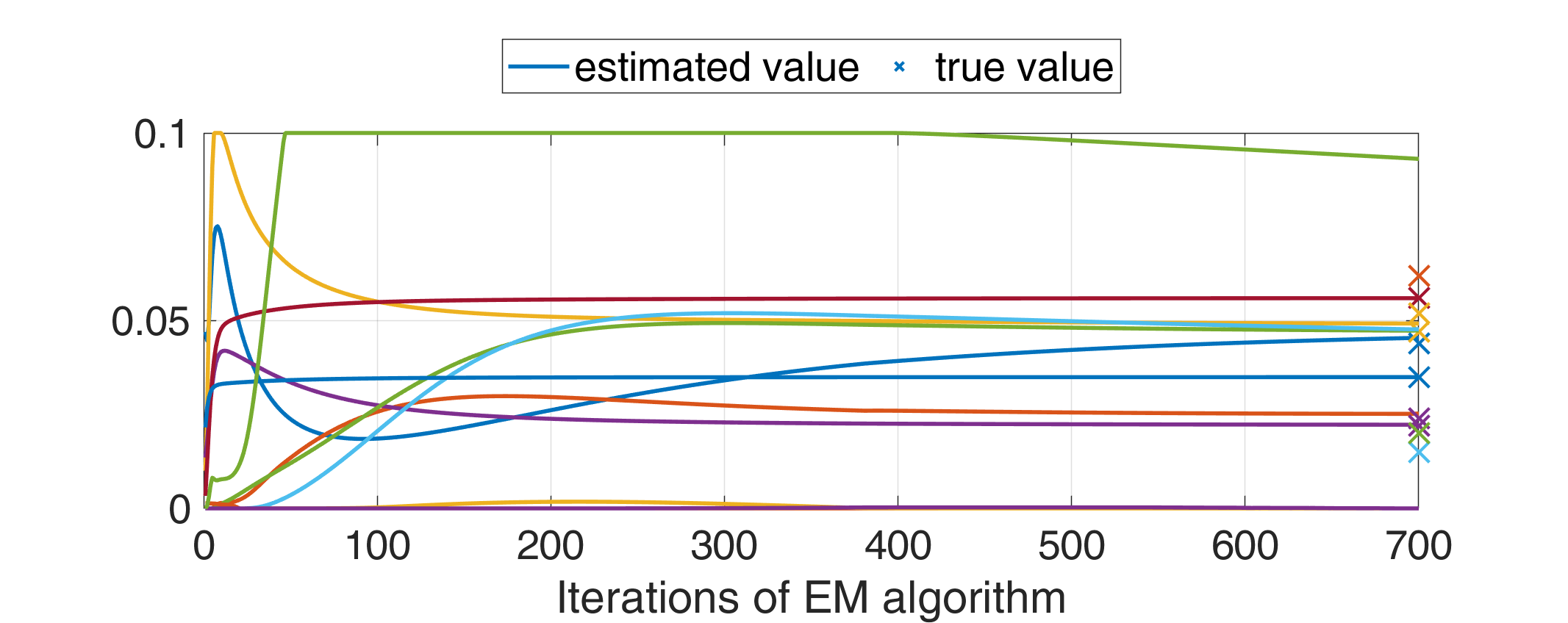
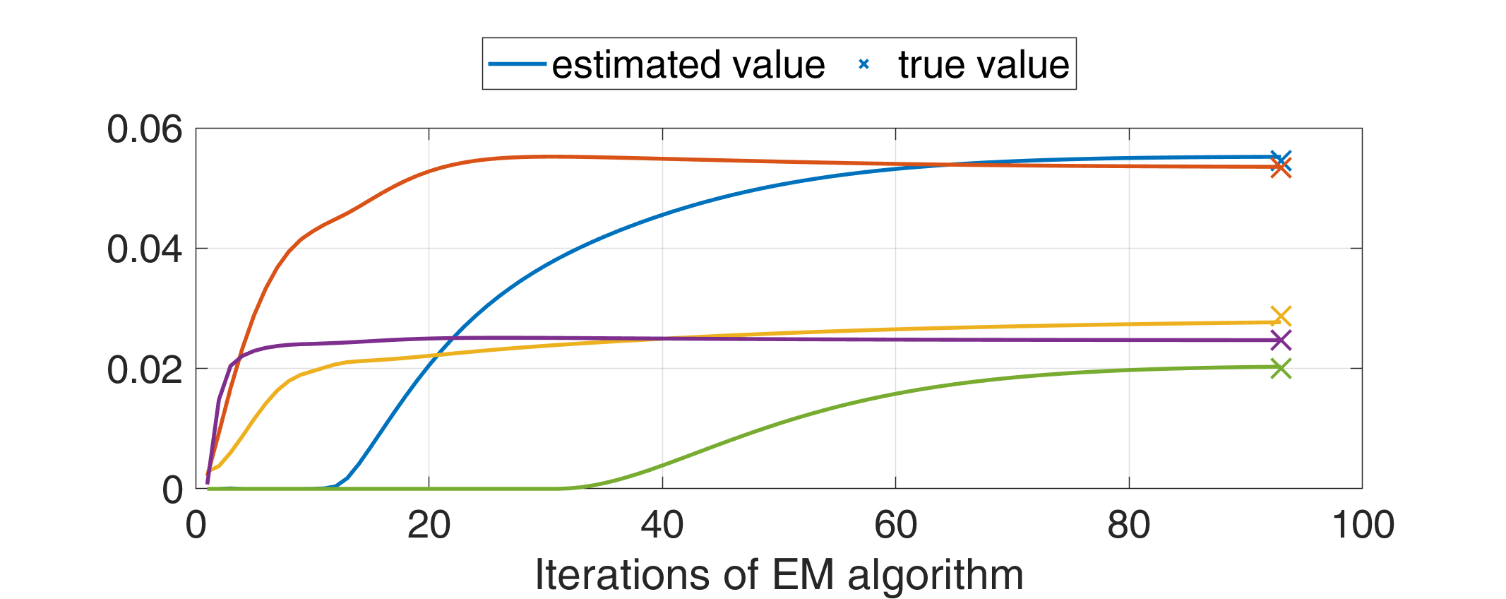
The convergence of parameters is studied in this subsection. We test two possibilities of parametrization of state matrix $A$. In the first case, we employ 12 parameters, which are specified in Table 1 and call this parametrization as weakly shared. The second studied model employs parametrization using only 5 parameters for description of matrix $A$, which we call strongly shared parametrization. Further there is one parameter connected with power losses $P_{i,t}$ in compartments representing IGBTs of the real module ($\boldsymbol{z}\in\mathbb{R}^{1}$) and parameters describing the estimator of state noise covariance matrix $Q$.

weakly shared parameters	true value	strongly shared parameters	true value
IGBT (layer 1) $\rightleftarrows$ IGBT (layer 1)	0.035	$k_{1}$	0.025
diode (layer 1) $\rightleftarrows$ diode (layer 1)	0.015
rectifier (layer 1) $\rightleftarrows$ rectifier (layer 1)	0.024
layer 2 (Cu layer) $\rightleftarrows$ layer 2 (Cu layer)	0.022	$k_{2}$	0.029
layer 3 $\rightleftarrows$ layer 3	0.044
layer 4 $\rightleftarrows$ layer 4	0.020
IGBT (layer 1) $\rightleftarrows$ layer 2 (Cu layer)	0.056	$k_{3}$	0.053
diode (layer 1) $\rightleftarrows$ layer 2 (Cu layer)	0.052
rectifier (layer 1) $\rightleftarrows$ layer 2 (Cu layer)	0.052
layer 2 (Cu layer) $\rightleftarrows$ layer 3	0.047	$k_{4}$	0.055
layer 3 $\rightleftarrows$ layer 4	0.062
layer 4 $\rightleftarrows$ ambient temperature	0.020	$k_{5}$	0.020

Table 1: Parameters of studied synthetic models

For identification purposes, the values of temperatures in compartments corresponding to selected IGBTs in the real power module (specifically 40 compartments out of all 117 compartments in the first layer), temperature of one selected compartment in layer 4 representing temperature sensor in the real power module and the ambient temperature represented by last compartment are observed according observation model (12). The input vector $\boldsymbol{P}_{1:N}$ is also assumed to be known. In this subsection, we know exactly the structure of both toy models (using weakly and strongly shared parametrization) and the true values of all parameters which we want to identified. Moreover, the process noise is neglected for better comparison.

The convergence of parameters $\boldsymbol{k}$ during identification process is depicted in Figure 3. It can be seen that in the case of strongly shared parametrization, all parameters converge to their true values (marked by crosses in the graph). In the case of weakly shared parametrization, the EM algorithm converges as well, but not to all true values of parameters $\boldsymbol{k}$. It can be caused by lack of information about temperatures in unobserved compartments (e.g. compartments representing diodes or rectifiers in the true power module). Despite the EM algorithm not converging to the true parameters in the weakly shared parametric model, the trend of temperature predicted by the identified model stays valid in some cases as can be seen in Figure 4, i.e. the identified model still explains measured temperatures relatively correctly. This conclusion is probably valid if no specific temperature fluctuation exists in unobserved compartments connected with remaining parts of model with poorly identified connections (e.g. a connection between rectifiers and Cu layer or a connection between diodes and Cu layer).

(a) Weakly shared parameters

(b) Strongly shared parameters

Figure 3: Convergence of values of parameters vector $\boldsymbol{k}$

Figure 4: Prediction of temperature trends – model generated with weakly shared parametrization and identified using strongly shared parametrization

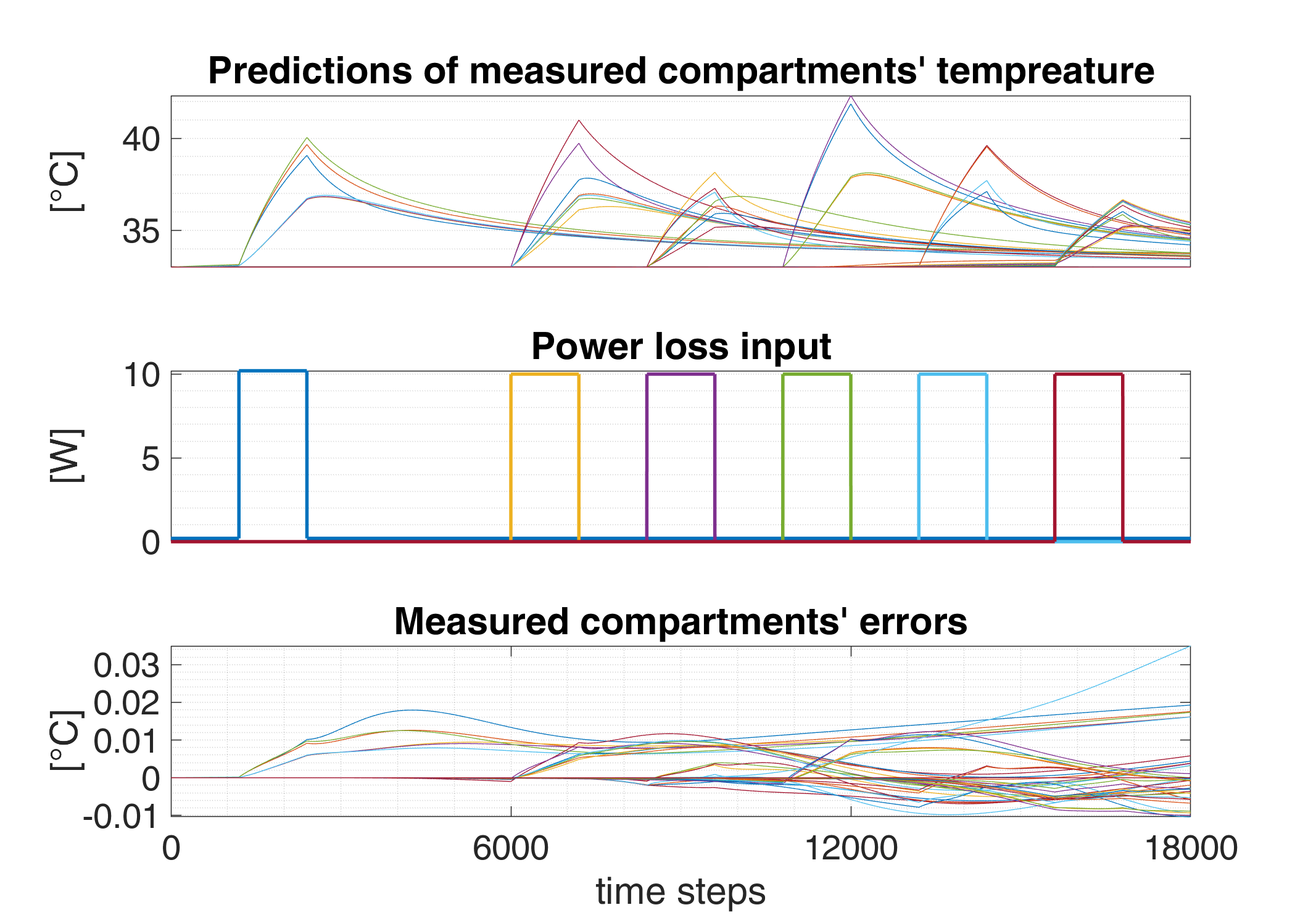
The error in prediction of temperature depicted in Figure 4 is not greater than 4% (maximum error of 0.3°C for temperature trend, where the difference between ambient temperature and maximum temperature is more than 9°C) for the synthetic model on relatively long-term prediction (for prediction of 18000 time steps from the initial value of temperature and with knowledge of the input vector $\boldsymbol{P}_{1:N}$ only). Note, that the same holds not only for the measured compartment, but for all compartments in the model as well.

5.2 Temperature prediction in dependency on covariance matrix structure

In this subsection we investigate the convergence properties of the EM algorithm for identification of the proposed mesh-based compartment thermal model in dependency on structure’s constraint of the process noise covariance matrix $Q$.

For the analysis of covariance matrix estimation, the weakly shared parametrization is employed to generate data, while during identification process strongly shared parametrization is assumed. It means that the identified model is thus not identical to the ground truth, although the structure (mesh-based discretization) of compartments is still the same. In other words, using various parametrization for generating data and for identifying model causes, that we do not know the true form of auxiliary matrices $\mathcal{A},\mathcal{B}$ and $\mathcal{C}$ in equations (6) and (7). Moreover, data are generated with process noise

$$\boldsymbol{w}_{t}\sim\mathcal{N}\left(\boldsymbol{w}_{t}|\boldsymbol{0},\sigma^{2}AA^{\prime}\right),$$ (26)

where $\sigma^{2}$ is set to value $10^{-4}$ and matrix $A$ is defined by (6).

We investigate three kinds of parametrization of the covariance matrix estimator similary as it is introduced in Section 4.4. For covariance structure’s constraint $Q_{\alpha LL^{\prime}+\beta I}^{r}=\alpha^{r}LL^{\prime}+\beta^{r}I_{n}$, elements $l_{i,j}$ of matrix $L\in\mathbb{R}^{n\times n}$ are defined as

$$l_{i,j}=\left\{\begin{array}[]{c}1\\ 0\end{array}\right. \begin{array}[]{l}\textrm{\qquad if }(\mathcal{I}\mathrm{\text{diag}(\mathcal{C}\boldsymbol{1})\mathcal{J}^{\prime}})_{i,j}\textrm{ is NOT }0\textrm{ and }j<n\\ \textrm{\qquad other}\end{array} \qquad i,j=1:n$$ (31)

where $\boldsymbol{1}$ is vector of all ones with the same dimension as vector $\boldsymbol{k}$ and where notation from (6) is used.

(a) State matrix $A$

(b) Matrix $LL^{\prime}$ used for covariance matrix $Q$ estimation

Figure 5: Illustration of matrix structure (white color corresponds to not zero element, black color corresponds to zero element)

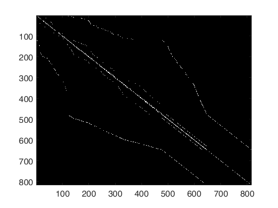
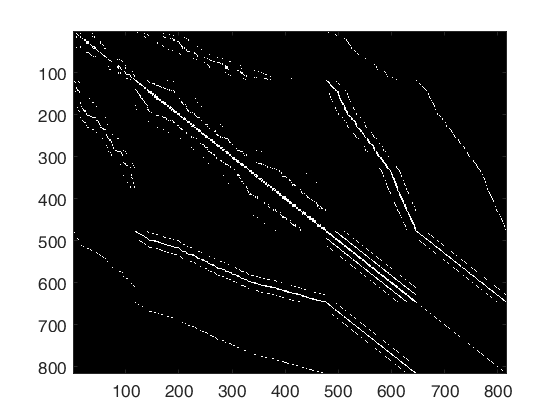
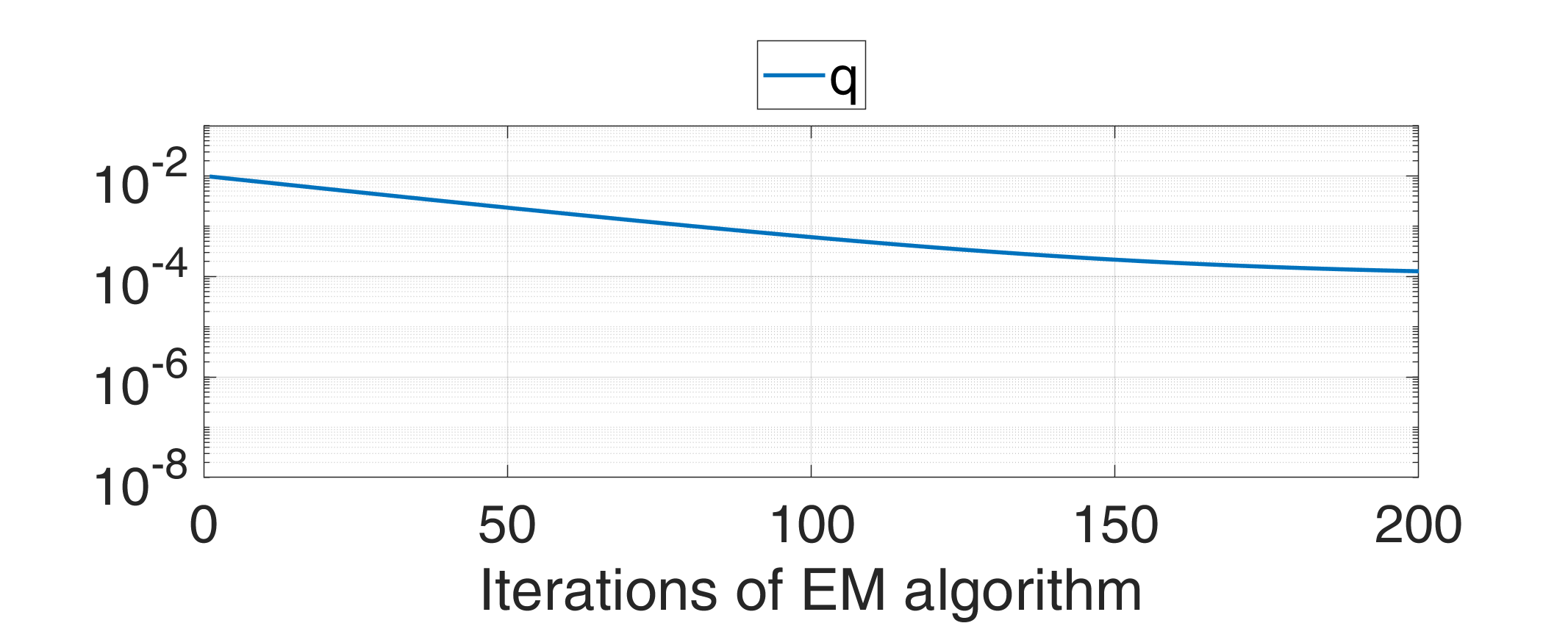
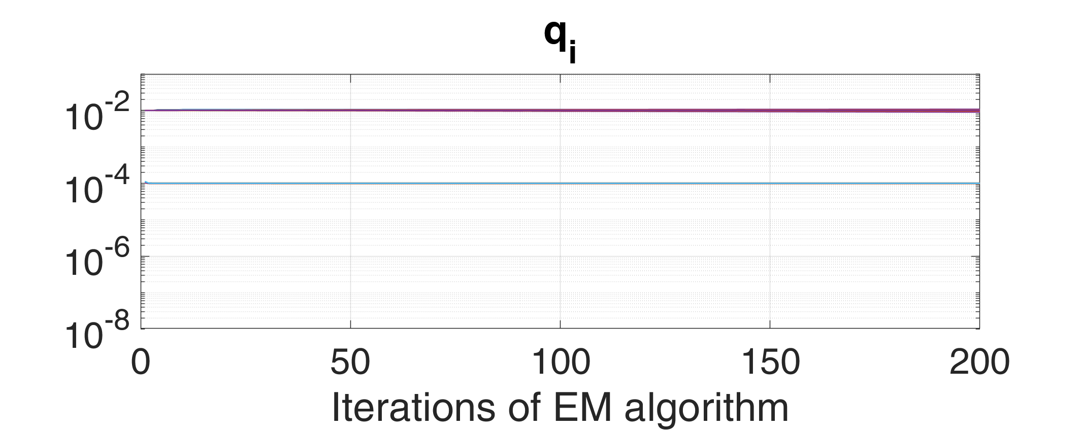
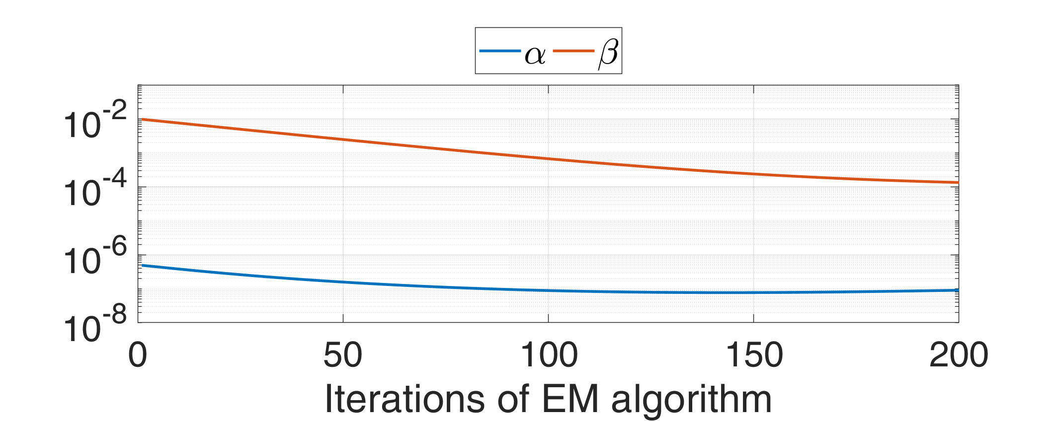
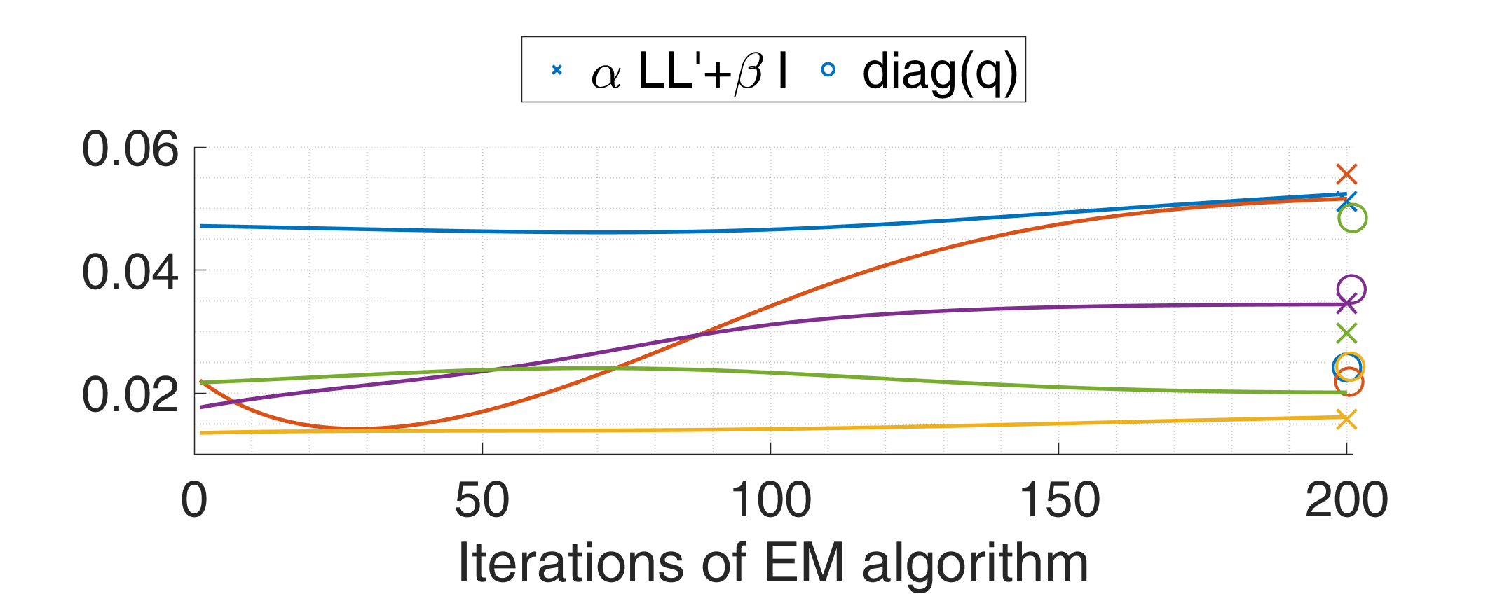
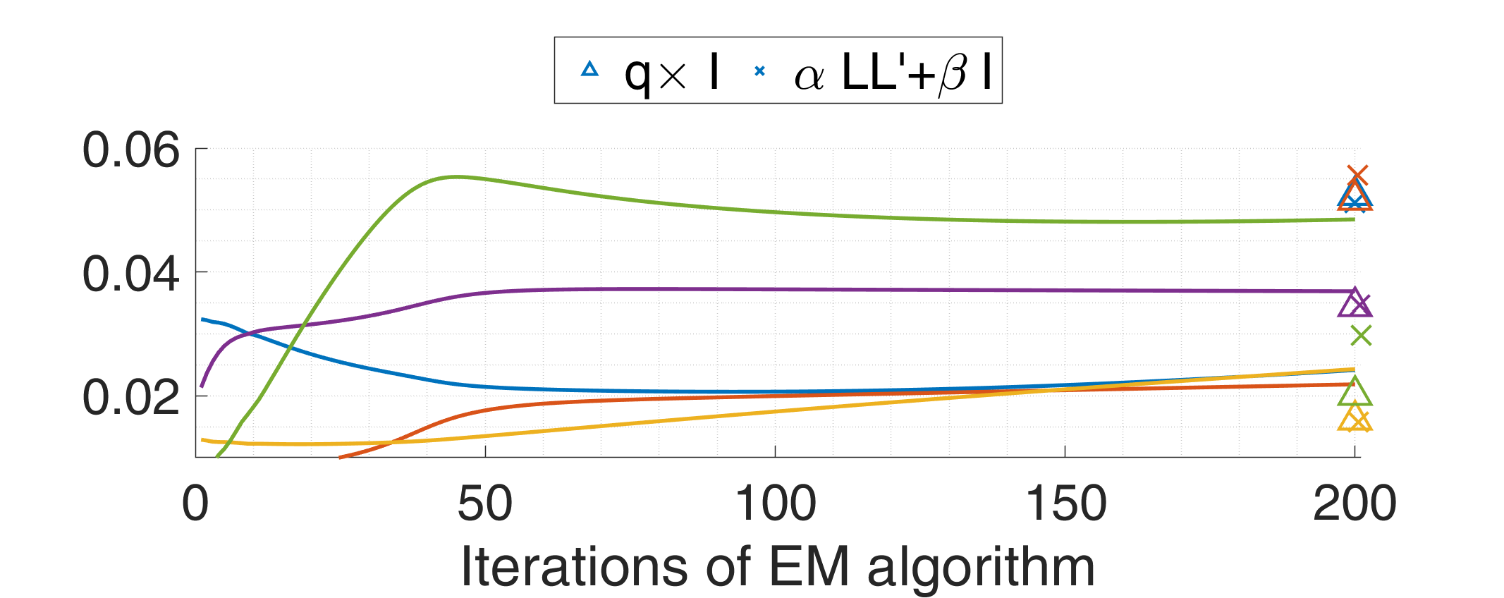
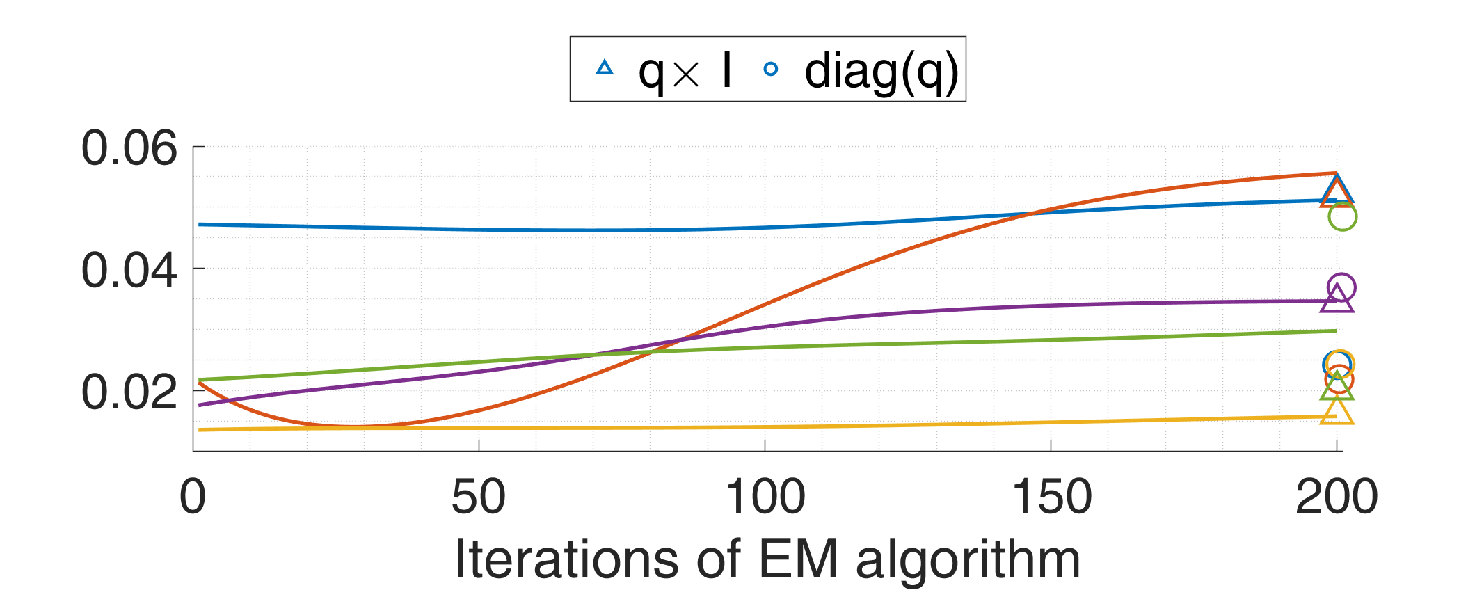
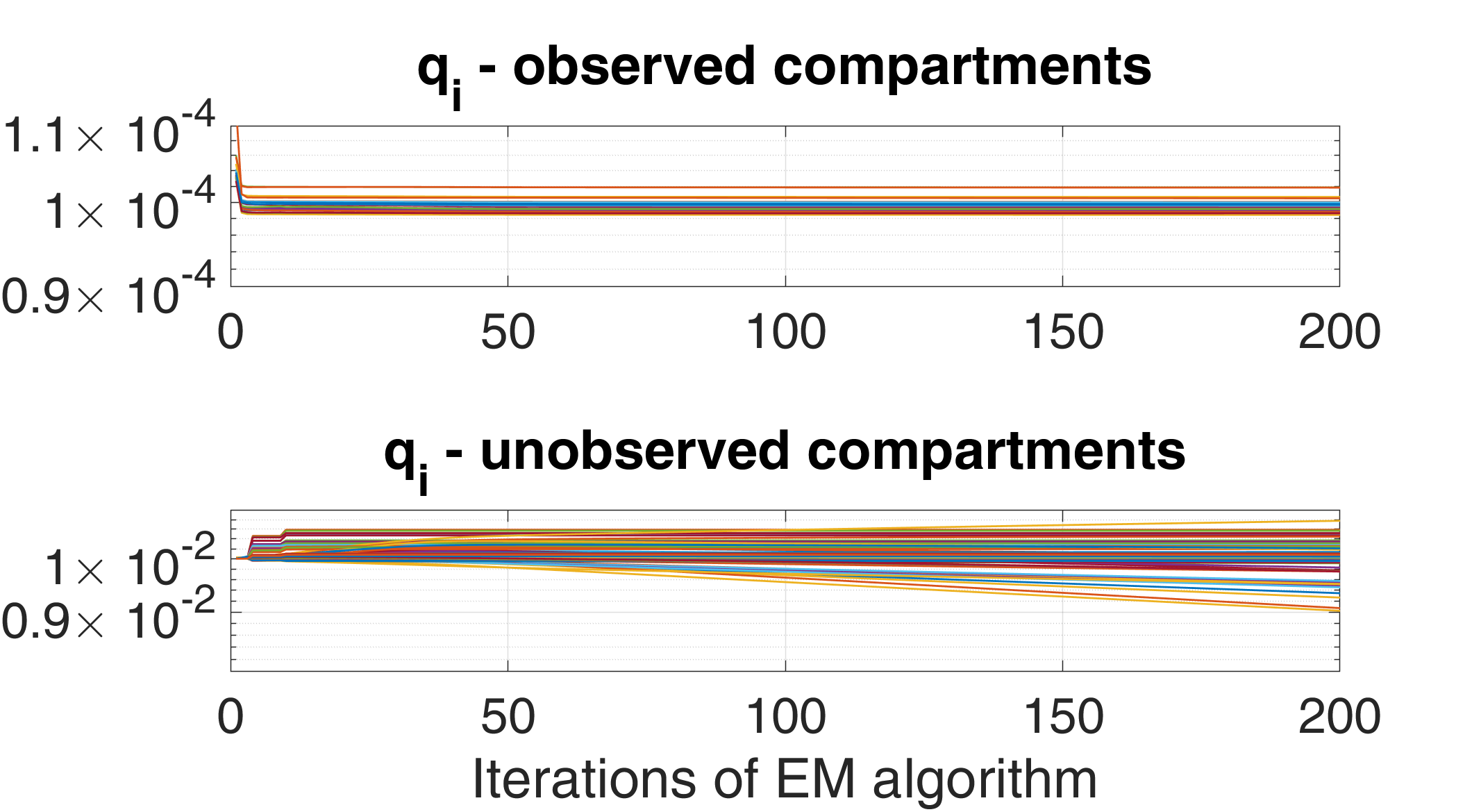
The convergence of parameters describing constrained covariance matrix $Q$ is depicted in Figure 6. The convergence of values of parameters vector $\boldsymbol{k}$ dependent on the choice of regularization of process noise covariance estimator is depicted in Figure 7. It can be seen, that models using constraints on covariance matrix $Q$ in forms $Q\overset{!}{=}qI_{n}$ and $Q\overset{!}{=}\alpha LL^{\prime}+\beta I_{n}$ give similar results and both of these form are sufficiently regularized. Moreover with knowledge of true covariance matrix (26) and being aware of matrix $A$ is diagonally dominant, we can claim, that these two approaches converge to the plausible values of covariance parameters. From this point of view, the constraint $Q\overset{!}{=}\text{diag}\left(\boldsymbol{q}\right)$ seems to be overparameterized, since the convergence of selected elements to the value $10^{-2}$, i.e. staying at the initial value, is not well-founded. Figure 8 can give an explanation of this phenomenon. Diagonal elements of covariance matrix taking higher values of variance ($10^{-2}$) are elements just corresponding to unobserved compartments. Elements converging to the true value of variance $10^{-4}$ are elements corresponding to the observed compartments. Thus due to lack of information about unobserved compartments, we are not able to identify the variance correctly using constraint $Q\overset{!}{=}\text{diag}\left(\boldsymbol{q}\right)$.

(a) Constraint $Q\overset{!}{=}qI_{n}.$

(b) Constraint $Q\overset{!}{=}\text{diag}\left(\boldsymbol{q}\right)$

(c) Constraint $Q\overset{!}{=}\alpha LL^{\prime}+\beta I_{n},$

Figure 6: Convergence of process noise covariance matrix estimation

(a) Constraint $Q\overset{!}{=}qI_{n}.$

(b) Constraint $Q\overset{!}{=}\text{diag}\left(\boldsymbol{q}\right)$

(c) Constraint $Q\overset{!}{=}\alpha LL^{\prime}+\beta I_{n},$

Figure 7: Convergence of values of parameters vector $\boldsymbol{k}$ in dependency on the constraint of process noise covariance matrix

Figure 8: Convergence of process noise covariance matrix estimation for the constraint $Q\overset{!}{=}\text{diag}\left(\boldsymbol{q}\right)$ – separation of elements corresponding to observed compartments and unobserved compartments

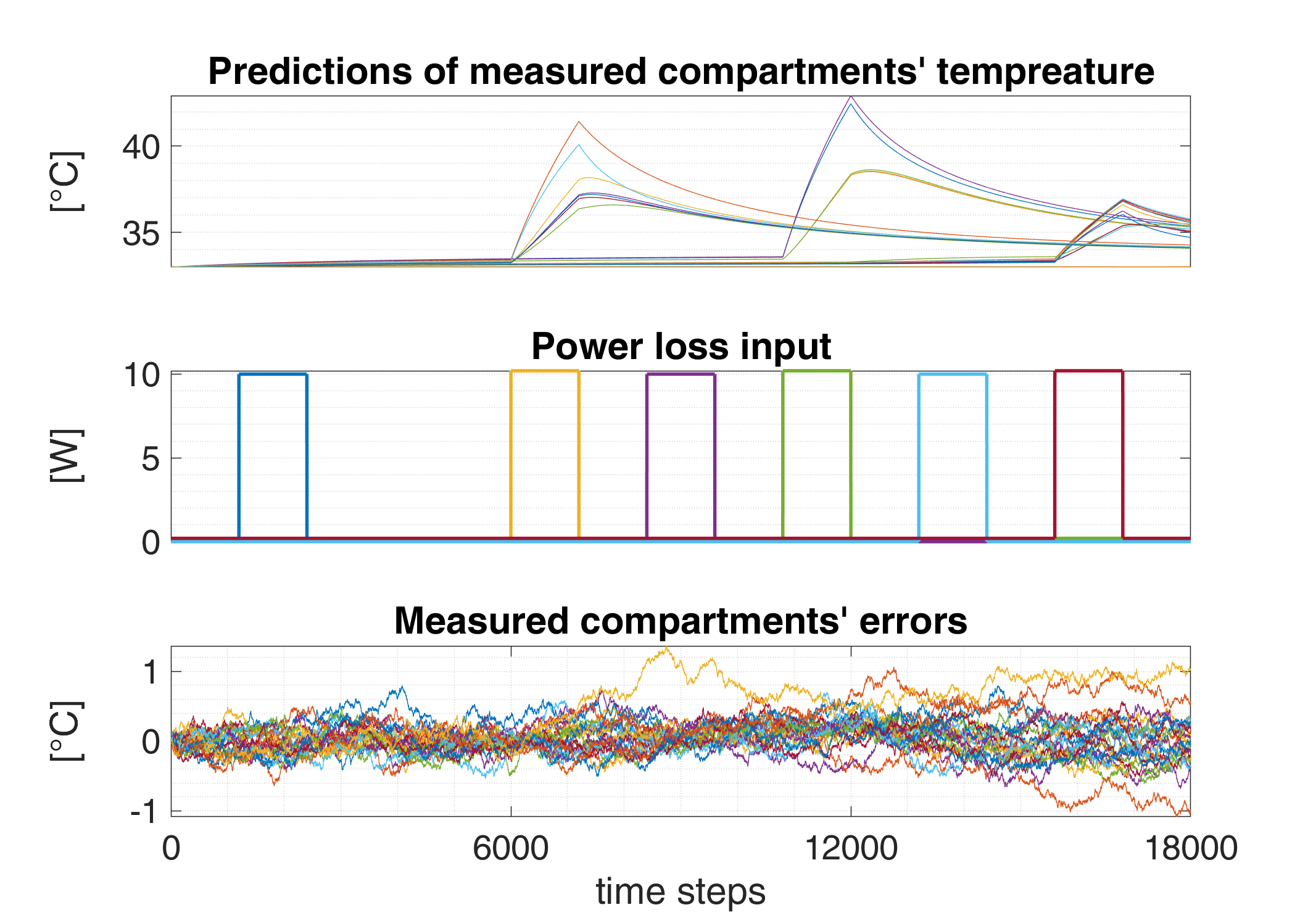
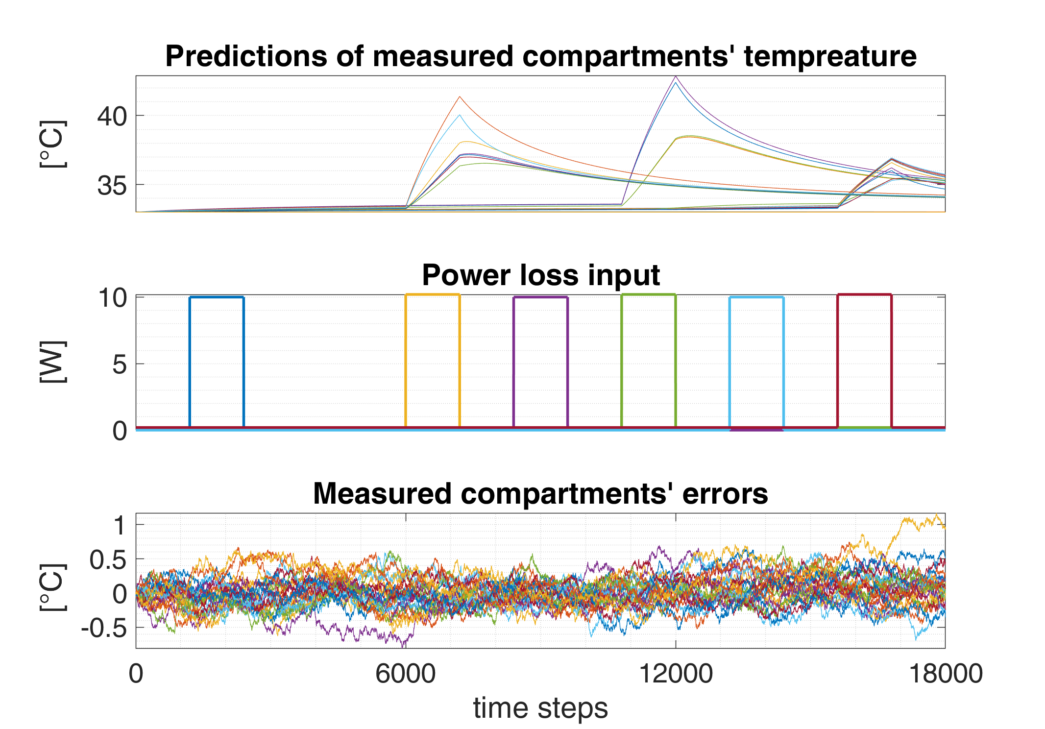
The long-term predictions of 18000 time steps using models identified with constrained covariance estimators $Q\overset{!}{=}qI_{n}$ and $Q\overset{!}{=}\alpha LL^{\prime}+\beta I_{n}$ respectively are depicted in Figure 9. Similar as in subsection 5.1, inputs of prediction are the initial values of temperatures and vector $\boldsymbol{P}_{1:N}$ only. On the contrary, we do not know the true parameterization during identification process (the parameterization used for identification is different from the one used for data generation). Nevertheless, the error of prediction is always smaller than 1 °C for temperature trends, where the difference between ambient temperature and maximum temperature is more than 10°C.

(a) Constraint $Q\overset{!}{=}qI_{n}.$

(b) Constraint $Q\overset{!}{=}\alpha LL^{\prime}+\beta I_{n},$

Figure 9: Temperature prediction and its errors

6 Conclusion

Mesh-based compartment thermal model and its identification procedure using Expectation-Maximization algorithm was proposed. Using steady-state covariance matrix in E-step of EM algorithm was suggested for speeding up the identification algorithm and constraints on structure of process noise covariance matrix in estimation procedure was investigated in detail.

Preliminary tests on synthetic data indicated applicability of the proposed thermal model and the identification approach. The selection of parametrization has a strong impact on the possibility to identify the model from incomplete temperature data. The strongly shared parameterized models are better identifiable and furthermore enable to explain more complicated models. However, the validation on real measured data is needed and ought to be carried out by authors in the near future.

Appendix A Expected terms for M-step

Expected terms necessary for equations (19) and (20) expressed using only statistics (17) obtained from a previous E-step:

$$\sum\limits_{t=1}^{N-1}E_{\Phi^{r}(T)}\left\{\Delta\boldsymbol{T}_{t}\Delta\boldsymbol{T}_{t}^{\prime}\right\}=\frac{1}{\Delta\tau^{2}}\left(XX^{\prime}-XZ^{\prime}-(XZ^{\prime})^{\prime}+ZZ^{\prime}\right)$$

$$\sum\limits_{t=1}^{N-1}E_{\Phi^{r}(T)}\left\{M_{t}^{\prime}Q^{-1}M_{t}\right\}=$$

$$\hskip 36.98866pt\text{=}\left[\begin{array}[]{cc}\mathcal{C}^{\prime}\left(\left(\mathcal{I}^{\prime}Q^{-1}\mathcal{I}\right)\circ\left(\mathcal{J}^{\prime}XX^{\prime}\text{$\mathcal{J}$}\right)\right)\mathcal{C}&-\mathcal{C}^{\prime}\left(\left(\mathcal{I}^{\prime}Q^{-1}\mathcal{B}\right)\circ\left(\mathcal{J}^{\prime}XU^{\prime}\right)\right)\mathcal{A}\\ -\mathcal{A}^{\prime}\left(\left(\mathcal{B}^{\prime}Q^{-1}\mathcal{I}\right)\circ\left(\left(XU^{\prime}\right)^{\prime}\mathcal{J}\right)\right)\mathcal{C}&\mathcal{A}^{\prime}\left(\mathcal{B}^{\prime}Q^{-1}\mathcal{B}\circ UU^{\prime}\right)\mathcal{A}\end{array}\right]$$

$$\sum\limits_{t=1}^{N-1}E_{\Phi^{r}(T)}\left\{M_{t}\boldsymbol{\theta}\boldsymbol{\theta}^{\prime}M_{t}^{\prime}\right\}=\left\{\boldsymbol{\theta}\boldsymbol{\theta}^{\prime}\equiv\left[\begin{array}[]{cc}\boldsymbol{kk}^{\prime}&\boldsymbol{kz}^{\prime}\\ \boldsymbol{zk}^{\prime}&\boldsymbol{zz}^{\prime}\end{array}\right]\right\}=$$

$$\hskip 36.98866pt=\mathcal{I}\left(\left(\mathcal{C}\boldsymbol{kk}^{\prime}\mathcal{C}^{\prime}\right)\circ\left(\mathcal{J}^{\prime}XX^{\prime}\text{$\mathcal{J}$}\right)\right)\mathcal{I}^{\prime}-\text{$\mathcal{B}$}\left(\left(\mathcal{A}\boldsymbol{zk}^{\prime}\mathcal{C}^{\prime}\right)\circ\left(\left(XU^{\prime}\right)^{\prime}\mathcal{J}\right)\right)\mathcal{I}^{\prime}+$$

$$\hskip 36.98866pt\hphantom{=}-\mathcal{I}\left(\left(\mathcal{C}\boldsymbol{kz}^{\prime}\mathcal{A}^{\prime}\right)\circ\left(\mathcal{J}^{\prime}XU^{\prime}\right)\right)\mathcal{B}^{\prime}+\text{$\mathcal{B}$}\left(\left(\mathcal{A}\boldsymbol{zz}^{\prime}\mathcal{A}^{\prime}\right)\circ UU^{\prime}\right)\mathcal{B}^{\prime}$$

$$\sum\limits_{t=1}^{N-1}E_{\Phi^{r}(T)}\left\{M_{t}Q^{-1}\Delta\boldsymbol{T}_{t}\right\}=\Delta t^{-1}\left[\begin{array}[]{c}-\mathcal{C}^{T}\text{diag}\left(\mathcal{J}^{T}\left(XZ^{\prime}-XX^{\prime}\right)\left(Q^{-1}\right)^{\prime}\mathcal{I}\right)\\ \mathcal{A}^{T}\text{diag}\left(\left(ZU^{\prime}-XU^{\prime}\right)^{\prime}\left(Q^{-1}\right)^{\prime}\mathcal{B}\right)\end{array}\right]$$

$$\sum\limits_{t=1}^{N-1}E_{\Phi^{r}(T)}\left\{\Delta\boldsymbol{T}_{t}\boldsymbol{\theta}^{\prime}M_{t}^{\prime}\right\}=\left\{\boldsymbol{\theta}\equiv\left[\begin{array}[]{c}\boldsymbol{k}\\ \boldsymbol{z}\end{array}\right]\right\}=$$

$$\hskip 36.98866pt=\Delta t^{-1}\left(XZ^{\prime}-XX^{\prime}\right)^{\prime}\mathcal{J}\text{diag}(-C\boldsymbol{k})\mathcal{I}^{T}+\Delta t^{-1}\left(ZU^{\prime}-XU^{\prime}\right)\text{diag}(\mathcal{A}\boldsymbol{z})\mathcal{B}^{T},$$

where symbol $\circ$ stands for Hadamard product, i.e. element-wise multiplication, and operator $\text{diag}(\cdot)$ applied on a vector creates diagonal matrix with the vector values on the main diagonal and operator $\text{diag}(\cdot)$ applied on a matrix extracts the main diagonal and the rest of elements replaces with zeros.

References

- [1] O. Wallscheid and J. Böcker. Global identification of a low-order lumped-parameter thermal network for permanent magnet synchronous motors. IEEE Transactions on Energy Conversion, 31(1):354–365, March 2016.
- [2] A. Boglietti, A. Cavagnino, D. Staton, M. Shanel, M. Mueller, and C. Mejuto. Evolution and modern approaches for thermal analysis of electrical machines. IEEE Transactions on Industrial Electronics, 56(3):871–882, March 2009.
- [3] X. Wang, X. Yuan, and Y. Sang. An improved lateral-coupling thermal impedance model of a half-bridge power module under inverter operations. In IECON 2019 - 45th Annual Conference of the IEEE Industrial Electronics Society, volume 1, pages 3142–3147, Oct 2019.
- [4] A. S. Bahman, K. Ma, and F. Blaabjerg. A lumped thermal model including thermal coupling and thermal boundary conditions for high-power igbt modules. IEEE Transactions on Power Electronics, 33(3):2518–2530, March 2018.
- [5] N. Simpson, R. Wrobel, and P. H. Mellor. An accurate mesh-based equivalent circuit approach to thermal modeling. IEEE Transactions on Magnetics, 50(2):269–272, Feb 2014.
- [6] Wenbo Wang, Xibo Yuan, P. L. Evans, and P. H. Mellor. Mesh-based lumped parameter model with mor for thermal analysis of virtual prototyping for power electronics systems with comparison to fdm. In 2017 IEEE 3rd International Future Energy Electronics Conference and ECCE Asia (IFEEC 2017 - ECCE Asia), pages 1037–1042, June 2017.
- [7] J. Ševčík, V. Šmídl, and M. Votava. Identification of thermal model of power module using expectation-maximization algorithm. In IECON 2019 - 45th Annual Conference of the IEEE Industrial Electronics Society, volume 1, pages 119–125, Oct 2019.
- [8] Suhas Patankar. Numerical heat transfer and fluid flow. CRC press, 2018.
- [9] A. Bondy and U.S.R. Murty. Graph Theory. Graduate Texts in Mathematics. Springer London, 2007.
- [10] Arthur P Dempster, Nan M Laird, and Donald B Rubin. Maximum likelihood from incomplete data via the em algorithm. Journal of the royal statistical society. Series B (methodological), pages 1–38, 1977.
- [11] Sam Roweis and Zoubin Ghahramani. An em algorithm for identification of nonlinear dynamical systems. 2000.
- [12] Herbert E Rauch, CT Striebel, and F Tung. Maximum likelihood estimates of linear dynamic systems. AIAA journal, 3(8):1445–1450, 1965.
- [13] John L Crassidis and John L Junkins. Optimal estimation of dynamic systems. Chapman and Hall/CRC, 2011.
- [14] Vasile Sima and Peter Benner. Numerical investigation of newton’s method for solving continuous-time algebraic riccati equations. In 2014 11th International Conference on Informatics in Control, Automation and Robotics (ICINCO), volume 1, pages 404–409. IEEE, 2014.
- [15] Wolfgang Mader, Yannick Linke, Malenka Mader, Linda Sommerlade, Jens Timmer, and Björn Schelter. A numerically efficient implementation of the expectation maximization algorithm for state space models. Applied Mathematics and Computation, 241:222–232, 2014.