Effective boundary conditions for magnetohydrodynamic flows with thin Hartmann layers.

Abstract

Here we build some effective boundary conditions to be used in numerical calculations in order to avoid the thin meshing usually required in problems involving Hartmann layers near a locally plane wall. Wall model are provided for both tangential and normal electric current density and velocity. In particular, a condition on the normal derivative of the tangential velocity is derived. A wide variety of problems is covered as the only restriction is that the magnetic Reynolds number has to be large at the scale of the Hartmann layer. The cases of perfectly conducting or insulating wall are examined, as well as the case of a thin conducting wall. The newest result is a condition on the normal velocity accounting for inertial effects in the Hartmann layer.

I Introduction

The flow of an electro-conducting fluid near a wall transverse to a magnetic field produces a specific boundary layer, the Hartmann layer, resulting from the balance between the Lorentz and the viscous force. This layer is generally very thin, which is problematic for a direct numerical resolution of the magnetohydrodynamic equations. The Hartmann layer thickness scales as the inverse of the magnetic field component orthogonal to the wall. Strong magnetic fields therefore dramatically reduce the layer thickness, to typically a few hundredths of mm in a liquid metal in a magnetic field of one Tesla, so that a very fine numerical mesh would be required for a direct computation. An insufficient resolution could spoil the whole computation as in some cases, the outer velocity is controlled by the total electric current passing through the layer, so an accurate description of the Hartmann layer is essential.

A convective flow in a rectangular elongated cavity alternatively has been modeled either meshing the layer or using a simple analytical model (using the classical linear model simply built on the balance between Lorentz and viscous forces (see for instance moreau90 ). It was found that 15 meshes within the layer were required in order to have a discrepancy smaller than $10\%$ from the outer velocity computed from the analytical model. Mück et. al. muck00 have also performed accurate numerical simulations using such a simple model. Similar difficulties would arise in many examples such as lithium blankets designed for nuclear fusion reactors (buhl96 ), where a liquid metal must evacuate heat under the strong transverse magnetic field used to confine the plasma, or in electromagnetic steerers where liquid steel is driven by a sliding magnetic field between transverse plates. Note finally the applications to the Earth liquid metal core, where we expect Hartmann layers with thickness less than one meter to occur at the contact with the mantle or with the solid metal inner core.

We propose here as an alternative approach to use an analytical model of the Hartmann layer, and to deduce effective boundary conditions for the core flow. Many previous works use a similar asymptotic approach, leading to a coupled analytical description of the core flow and boundary layers. Such fully analytical solutions are however generally limited to linear problems, e.g. Hunt and Shercliff hunt71 for duct flows, Walker walker81 for convection. A two-dimensional evolution equation for a 2D core flow relying on a similar idea is proposed in sm82 . Pothérat et Al. psm00 extended such effective 2D models to the case of moderate magnetic fields, taking into account recirculating secondary flows in the Hartmann layer. Here, we consider again the same effects, but with the goal of extracting an effective boundary condition for the core flow, without any assumption on its dynamics (it is not necessarily described as a two-dimensional flow).

Our approach here is quite general, with possibly non-uniform or time varying magnetic fields and various wall electric conditions, as presented in section 2. We use a systematic expansion for the Hartmann layer valid for large magnetic fields, and the matching with the core provides the requested effective boundary conditions. The zero order classical Hartmann layer is recalled in section 3, and effective boundary conditions are deduced. It is shown that in many cases, one can just forget the Hartmann layer and allow the fluid to slip on the wall.

However this is not always sufficient, in particular in the case of insulating walls. Thus the electric current sheet generated in the Hartmann layer transmits a friction effect in the core. This is taken into account by an effective condition on the normal current density. Similarly a normal velocity is generated in the Hartmann layer, due to the recirculating flows induced by inertial effects. This appears as a higher order correction on the Hartmann layer, derived in section 4. In the case of Coriolis effects, these effects are modified as the Hartmann layer is transformed into Hartmann-Ekman layer, as discussed in section 5.

II Description of the system

Let us consider an incompressible fluid with density $\rho$, kinematic viscosity $\nu$, conductivity $\sigma$ in a magnetic field $\mathbf{B}\left(\mathbf{x,}t\right)$ possibly depending on time $t$ and position vector $\mathbf{x}$. All variables are non-dimensional, using a typical magnetic field value $B_{0}$, a velocity $U$, a scale $a$ of the fluid domain. The time is normalized by the advective time scale $a/U$. The dynamics then depend on three non-dimensional parameters, the Hartmann number $Ha$, the interaction parameter $N$ and the magnetic Reynolds number $Rm$,

$$Ha=(\tfrac{\sigma B_{0}^{2}}{\rho}\tfrac{a^{2}}{\nu})^{1/2}\;\;,\;\;N=\tfrac{\sigma B_{0}^{2}}{\rho}\tfrac{a}{U}\;\;,\;\;Rm=\mu\sigma Ua.$$ (1)

The Hartmann number and interaction parameter compare the electromagnetic forces respectively to viscosity and inertia. Note that the hydrodynamic Reynolds number $Re$ can be expressed as $Re=Ha^{2}/N$, while the magnetic Reynolds number $Rm$ compares advection and diffusion of the magnetic field.

The non-dimensional velocity field $\mathbf{u}$ satisfies the Navier-Stokes equations

$$\partial_{t}\mathbf{u+u.\nabla}\mathbf{u}={\ \tfrac{1}{Re}}\mathbf{\Delta u}+N\mathbf{j\times B}-N{\nabla p},$$ (2)

$$\mathbf{\nabla.u}=0,$$ (3)

with an electromagnetic force proportional to the current density $\mathbf{j}$, normalized by its estimate $\sigma UB_{0}$. The pressure $p$ has been normalized by its estimate $N\rho U_{0}^{2}$, corresponding to a balance between pressure and electromagnetic forces. The electric current and magnetic field satisfy the Ohm’s law and the equations of magnetic induction, in non-dimensional form,

$$\mathbf{j}=\mathbf{E}+\mathbf{u\times B},$$ (4)

$$\nabla\times\mathbf{E}=-\partial_{t}\mathbf{B},$$ (5)

$$\mathbf{\nabla\times B=}Rm\,\mathbf{j},$$ (6)

$$\mathbf{\nabla.B}=0.$$ (7)

Note that taking the curl of the Ohm’s law (4) and using (5), we get :

$$\nabla\times\mathbf{j}=-\partial_{t}\mathbf{B}-\mathbf{u.\nabla B}+\mathbf{B.\nabla u}.$$ (8)

The boundary condition for the velocity is the classical no-slip condition

$$\mathbf{u}=0.$$ (9)

For the magnetic field, there is a condition of continuity with the outside of the normal component $\mathbf{B.n}$ ($\mathbf{n}$ is the normal to the wall). There is also a condition on the tangential components of $\mathbf{B}$, related to the electrical boundary conditions by the induction law (6). Denoting $\mathbf{j_{W}}$ the current density at the wall, the tangential projection of the magnetic field is determined from the normal current $\mathbf{j_{W}.n}$ on the whole boundary, while the normal derivative of this tangential magnetic field is proportional to the tangential projection of $\mathbf{j_{W}}$. We shall consider four cases:

1. insulating walls, $\mathbf{j_{W}.n}$=0,

2. electrodes controlling the injected current $\mathbf{j_{W}.n}=j_{I}$ is given,

3. perfectly conducting walls $\mathbf{j_{W\|}}=0$,

4. thin conducting walls, with conductance $\Sigma_{W}\sigma a$ (so that $\Sigma_{W}$ is non-dimensional). Then the tangential electric field $\mathbf{E_{\|}}$, which is continuous at the boundary, is proportional to the surface current density $\mathbf{J_{W}}$ along the wall shell, $\mathbf{E_{\|}=J_{W}}/\Sigma_{W}$. The current conservation in this shell yields $\nabla_{\|}.\mathbf{J_{W}}=j_{I}-j_{Wz}$, where $j_{I}$ is a current density possibly injected on the shell by electrodes from outside. Then, using the Ohm’s law (4) at the wall, with $\mathbf{u}=0$, we get the electric boundary condition

   $$\nabla_{\|}.(\Sigma_{W}\mathbf{j_{W\|}})+\mathbf{j_{W}.n}=j_{I},$$ (10)

   which in fact covers the four cases. The case of insulating walls or imposed normal current is obtained with $\Sigma_{W}=0$ and the case of perfectly conducting walls with $\Sigma_{W}\rightarrow\infty$.

Near the walls with non-zero transverse magnetic field $\mathbf{B.n}$, a Hartmann boundary layer occurs. It is dominated by a balance between the electromagnetic force, pressure force and viscosity (the three terms in the right hand side of (2)). The thickness of this layer is in $a(Ha\mathbf{B.n})^{-1}$, which we suppose to be much smaller than $a$. This is verified in most cases of interest. We furthermore assume that the magnetic field variation $\delta\mathbf{B}$ across this layer is small, $\delta\mathbf{B}\ll\mathbf{B}$. Then the magnetic field can be assumed given when the dynamics of the boundary layer is studied. This is satisfied when the magnetic Reynolds number at the scale of the Hartmann number is small, $Rm/Ha\ll 1$, a condition which is in practice always verified, even if $Rm$ is large. In some engineering applications (e.g. in induction pumps), a magnetic field oscillation is externally imposed with frequency $f$. Then our analysis applies if the skin depth $(\mu\sigma f)^{-1/2}$ remains larger than the Hartmann layer thickness $a(Ha\mathbf{B.n})^{-1}$, so that again the magnetic field can be considered as uniform across the Hartmann layer.

Inertial effects are assumed small in the Hartmann layer, which is satisfied for high interaction parameters $N$. We shall consider the perturbative effects of inertia, resulting in recirculation effects, so our analysis extends in reality for values of $N$ close to unity. In summary our analysis applies when

$$Ha\;\mathbf{B.n}\gg 1,\quad N\gg 1,\quad\frac{Rm}{Ha}\ll 1,\quad f\ll\dfrac{Ha^{2}}{\mu\sigma a^{2}}.$$ (11)

Furthermore we shall assume that the curvature radius of the walls is large with respect to the thickness $aB_{0}(Ha\mathbf{B.n})^{-1}$ of the Hartmann layer, so that the latter can be assumed locally plane.

In addition we shall separately discuss the case with strong Coriolis force, as relevant in a planetary liquid metal core. Then Hartmann-Ekman layers are obtained instead of Hartmann layers.

III The Hartmann Layer.

III.1 The equation of motion in the Hartmann layer.

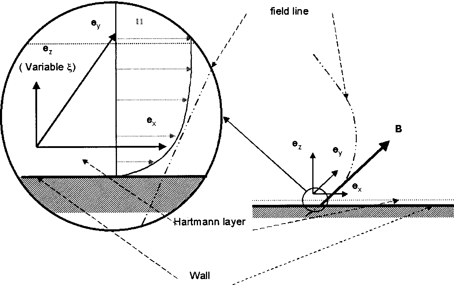
Figure 1: Geometric configuration

In the Hartmann boundary layer, the normal derivative dominates the tangential ones. We choose an orthonormal reference frame ($\mathbf{e}_{x},\mathbf{e}_{y},\mathbf{e}_{z}$), where $\mathbf{e_{z}}$ is the unit vector normal to the wall, and the origin is chosen so that the wall corresponds to the surface $z=0$. We define the stretched non-dimensional coordinate $\xi=Ha\;z$, which remains of order one in the Hartmann layer, and denote the fields by the superscript $\hat{()}$, to specify that they are functions of this stretched coordinate.

We assume that the wall curvature is sufficiently small, so that the Hartmann layer can be calculated with the cartesian coordinates $(x,y,\xi)$, where the origin of $\xi$ is at the wall. In further discussions, vectors belonging to the plane of the wall are referred as tangential whereas vectors orthogonal to the wall are called normal

The velocity $\mathbf{u}$ is then decomposed in its tangential projection, denoted $\mathbf{{u}_{\|}}$, and normal component, denoted ${w}$.

With these conventions, the continuity equation (3) rewrites

$$-\dfrac{1}{Ha}\mathbf{\nabla}_{\|}.\mathbf{\hat{u}_{\|}}=\partial_{\xi}\hat{w},$$ (12)

so that the normal velocity $\hat{w}$ is of order $\frac{1}{Ha}$

The tangential projection of the Navier-Stokes equation yields

$$\tfrac{1}{N}\left[\left(\partial_{t}+\mathbf{\hat{u}.\nabla}_{\|}+Ha\,\hat{w}\,\partial_{\xi}\right)\mathbf{\hat{u}_{\|}}\right]-\tfrac{1}{Ha^{2}}\mathbf{\Delta}_{\|}\mathbf{\hat{u}}$$

$$=-\mathbf{\nabla}_{\|}\hat{p}+\partial_{\xi\xi}^{2}\mathbf{\hat{u}_{\|}}+B_{z}\mathbf{\hat{\jmath}\times e}_{z}+\hat{\jmath}_{z}\mathbf{e}_{z}\times\mathbf{B}_{\|}.$$ (13)

The normal component of the Navier-Stokes equation yields, to an excellent approximation a balance between normal pressure and electromagnetic force, namely

$$\mathcal{O}(N^{-1}Ha^{-1})=-\partial_{z}p+\mathbf{\hat{\jmath}_{\|}\times B_{\|}}.$$ (14)

The electric current conservation writes :

$$-\dfrac{1}{Ha}\mathbf{\nabla}_{\|}\mathbf{.\hat{\jmath}_{\|}}=\partial_{\xi}\hat{\jmath}_{z}.$$ (15)

The curl of the Ohm’s law (8) is written in terms of the stretched variable as

$$\dfrac{1}{Ha}\left[\left(\mathbf{e}_{z}\times\mathbf{\nabla}_{\|}\right)\hat{\jmath}_{z}-\dfrac{d}{dt}\mathbf{B}_{\|}+\left(\mathbf{B}_{\|}\mathbf{.\nabla}\right)\mathbf{\hat{u}_{\|}}\right]$$

$$=\mathbf{e}_{z}\times\partial_{\xi}\mathbf{\hat{\jmath}_{\|}}-B_{z}\partial_{\xi}\mathbf{\hat{u}_{\|}},$$ (16)

where $\frac{d}{dt}\equiv\partial_{t}+\mathbf{\hat{u}.\nabla}_{\|}$ is the advection operator.

The Hartmann layer solution is supposed to match the core solution of the motion equation. The latter differs from the Hartmann layer solution by its typical normal lenghscale which is $\mathcal{O}\left(1\right)$ and to which the normal coordinate $z$ normalized by $a$ is associated. Then, the core solution does not satisfy the boundary condition at the wall. Moreover, the validity domain of the boundary layer solution does not extend to the core, so that the matching of the two solutions has to occur at an intermediate scale $\zeta\left(Ha^{-1}\right)$, possibly depending on $Ha$, satisfying Kaplun54 :

$$Ha^{-1}\ll\zeta\left(Ha^{-1}\right)\ll 1.$$ (17)

We shall here denote the functions of the core coordinate $z$ by the superscript $\check{()}$, to distinguish them from the functions of the stretched coordinate $\xi$. Matching the core solution to the boundary solution at the intermediate scale is achieved by the asymptotic condition for any quantity $g$ :

$$\lim_{\begin{subarray}{c}Ha^{-1}\rightarrow 0\\ z_{\zeta}fixed\end{subarray}}\check{g}\left(\zeta z_{\zeta}\right)-\hat{g}\left(Ha\zeta z_{\zeta}\right)=0$$ (18)

for an appropriate intermediate scale $\zeta(Ha^{-1})$ and for any value of the argument $z_{\zeta}$. When the function $\hat{g}$ decays exponentially to a constant, we can just replace (18) by the simpler condition

$$\lim\limits_{{}_{z\rightarrow 0}}{\check{g}}\left(z\right)=\lim\limits_{{}_{\xi\rightarrow\infty}}{\hat{g}}\left(\xi\right)$$ (19)

However, we shall find that some perturbative terms, of order $N^{-1}$ or $Ha^{-1}$ for instance, increase with $\xi$, so that $\lim\limits_{{}_{\xi\rightarrow\infty}}{\hat{g}}\left(\xi\right)=\infty$ and the more general condition (18) must be used instead of (19).

III.2 The classical Hartmann layer

The zero order equations are given by neglecting the terms in $1/N$ and $1/Ha$ in (12), (13), (15), (16): we only keep the right-hand terms, of order unity. Taking into account the no slip condition at the wall, (12) and (15) yield :

$$\begin{array}[]{cc}\hat{w}=0,&\hat{j_{z}}=j_{Wz}.\end{array}$$ (20)

By continuity with the core, this gives the effective conditions $\check{w}(0)=0$ and $\check{j_{z}}(0)=j_{W}z0$, which just reproduce the wall conditions, as expected across the thin Hartmann layer.

Using (20), (13) and (16) are simplified. Integrating (16) with condition $\mathbf{\hat{\jmath}_{\|}}(0)=\mathbf{j_{W\|}}$ yields a relation between the tangential current density and velocity

$$\mathbf{\hat{\jmath}_{\|}}(\xi)=\mathbf{j}_{W\|}-B_{z}\left(\mathbf{e}_{z}\times\mathbf{\hat{u}_{\|}}\right),$$ (21)

which just expresses the Ohm’s law (4) with a constant tangential electric field across the Hartmann layer. Eliminating the current density with (13) yields an equation for $\mathbf{\hat{u}_{\|}}\left(\xi\right).$ The latter can be solved using the no-slip condition (9) for the tangential velocity and the matching condition (18), which at zero order simplifies in $\lim\limits_{{}_{z\rightarrow 0}}\mathbf{\check{u}}\left(z\right)=\lim\limits_{{}_{\xi\rightarrow\infty}}\mathbf{\hat{u}}\left(\xi\right)$, so that finally we get the classical Hartmann velocity and current density Hartmann profiles,

$$\mathbf{\hat{u}_{\|}}\left(\xi\right)=\mathbf{\check{u}}_{\|}(0)\left[1-e^{-B_{z}\xi}\right],$$ (22a)

$$\mathbf{\hat{\jmath}}_{\|}\left(\xi\right)=\mathbf{j}_{W\|}+B_{z}\mathbf{\check{u}_{\|}}\left(0\right)\times\mathbf{e}_{z}\left[1-e^{-B_{z}\xi}\right].$$ (22b)

The matching with the core yields the conditions :

$$\mathbf{\check{u}_{\|}}\left(0\right) = B_{z}^{-1}\mathbf{j}_{W\|}\mathbf{\times e}_{z}-B_{z}^{-2}j_{Wz}\mathbf{B}_{\|}\times\mathbf{e}_{z}-B_{z}^{-2}\mathbf{\nabla}_{\|}p,$$

$$\mathbf{\check{j}_{\|}}\left(0\right) = \mathbf{j}_{W\|}+B_{z}\mathbf{\check{u}_{\|}}\left(0\right)\times\mathbf{e}_{z}.$$ (24)

By eliminating $\mathbf{j}_{W\|}$ in these two relations, and using the matching $\check{j_{z}}(0)=j_{Wz}$, we get :

$${B_{z}}\mathbf{\check{j}_{\|}}(0)-\mathbf{B_{\|}}(0)\check{j_{z}}(0)-B_{z}^{-1}\mathbf{\nabla}_{\|}p\times\mathbf{e}_{z}=\mathcal{O}\left(N^{-1}\right).$$ (25)

This relation just expresses the balance, in tangential projection, between the electromagnetic force $\mathbf{j\times B}$ and the pressure force.

III.3 Effective boundary conditions for the core

We get effective boundary conditions for the core at $z\to 0$ by matching these results on Hartmann layer for $\xi\to\infty$, or more precisely using the condition (18).

First, the impermeability condition $w=0$ is just transmitted to the core boundary thanks to (20). We need two additional effective boundary conditions, one condition for the current, and one hydrodynamic condition in order to replace the no-slip wall condition. These are provided by the continuity of $j_{z}$ and the two relations (24) and (25).

In the case of a fixed injected current density $j_{Wz}$, for instance with insulating walls, this condition on $j_{Wz}$ is just transmitted to the core boundary like the normal velocity. This allows to solve the equations for the magnetic field and electric current, providing $\mathbf{\check{j}_{\|}}$ near the boundary. Then (25) provides the required hydrodynamic condition, in terms of pressure. In some cases the typical pressure effects are of order $N^{-1}$, so this condition is no more effective, and this case will be discussed below. The additional relation (24) is not needed for the effective boundary conditions: it just determines the wall tangential current density $\mathbf{j}_{W\|}$.

In the case of a perfectly conducting wall, $\mathbf{j}_{W\|}=0$, then (24) and (25) provide relationships between $\mathbf{\check{j}_{\|}}(0)$, $\check{j_{z}}(0)$, pressure gradient and velocity.

In the case of a thin wall, combining the divergence of (24) and (10) gives :

$$\nabla_{\|}.[\Sigma_{W}B_{z}(\mathbf{\check{u}_{\|}(}0\mathbf{)\times e_{z})}]=(\check{j}_{z}(0)-j_{I})+\nabla_{\|}.[\Sigma_{W}\mathbf{\check{j}_{\|}}(0)],$$ (26)

which has to be used in combination with the hydrodynamic condition (25).

As already noticed, this condition is only relevant if the pressure effects are of order unity. When they are not imposed from the outside, like in ducts, pressure gradients rather tend to scale as $\rho U^{2}$, or $N^{-1}$ in non-dimensional units, so that (25) does not provide any hydrodynamic condition. It just states that the current is nearly aligned with the magnetic field, so that the electromagnetic force $\mathbf{j\times B}$ is weaker (by a factor at least $N$) than expected from direct dimensional analysis. The effective hydrodynamic condition can be obtained in all cases from the curl of the Ohm’s law (8) at $z=0$ :

$$\partial_{z}\mathbf{\hat{u}}_{\|}-B_{z}^{-1}\left(\mathbf{u}_{\|}\mathbf{.\nabla}_{\|}\right)\mathbf{\check{B}_{\|}}+B_{z}^{-1}\left(\mathbf{B}_{\|}\mathbf{.\nabla}_{\|}\right)\mathbf{\check{u}_{\|}}$$

$$=-B_{z}^{-1}\left[\left(\mathbf{e}_{z}\times\mathbf{\nabla}_{\|}\right)\check{j}_{z}-\partial_{t}\mathbf{B}_{\|}+B_{z}^{-1}\partial_{z}\mathbf{\check{j}}\mathbf{\times e}_{z}\right].$$ (27)

The normal derivative $\partial_{z}\mathbf{\check{j}}\left(0\right)$ can be expressed as a function of the current density and the magnetic field by differentiating the Navier-Stokes equation in the core at leading order (III.2), with respect to $z$. In addition, the pressure can be eliminated using (14), the vertical component of the Navier Stokes equation in the core. Then (27) becomes :

$$\partial_{z}\mathbf{\check{u}}_{\|}=-B_{z}^{-1}\left[\begin{array}[]{c}\left(\mathbf{e}_{z}\times\mathbf{\nabla}_{\|}\right)\check{j}_{z}-\frac{d}{dt}\mathbf{B}_{\|}\mathbf{+}\left(\mathbf{B}_{\|}\mathbf{.\nabla}\right)\mathbf{\check{u}}\\ +\partial_{z}\mathbf{\check{j}}_{\|}\left(0\right)\times\mathbf{e}_{z}\end{array}\right],$$ (28)

where $\partial_{z}\mathbf{\check{j}}_{\|}\left(0\right)\times\mathbf{e}_{z}$ is obtained from the solution of the system formed with (25) and (14). An alternate way to obtain a condition on $\partial_{z}\mathbf{\hat{u}}_{\|}(0)$. This relation relates an effective boundary condition on velocity to the boundary condition for the electric current. In the case of a magnetic field normal to the wall, $\mathbf{B}_{\|}=0$, it reduces to

$$\partial_{z}\mathbf{\check{u}_{\|}}^{\left(0\right)}\left(0\right)=B_{z}^{-1}\left(\mathbf{e}_{z}\times\mathbf{\nabla}_{\|}\right)j_{zW}^{\left(0\right)}$$ (29)

and $\partial_{z}\mathbf{\hat{u}}_{\|}=0$ for an insulating wall. Note that this effective boundary condition has been already derived by Sommeria and Moreau (1982) to justify the two-dimensional dynamics of turbulence observed in duct flows with insulating walls and transverse magnetic field. When an electric current is injected through electrodes at the boundary, a normal shear is introduced as indicated by (29). This corresponds to the existence of a shear layer parallel to the magnetic field, propagating from the electrode along magnetic field lines into the core flow.

Up to now, the effective boundary conditions could be obtained without explicit calculation of the Hartmann layer. We could have just used the impermeability condition for velocity and continuity of the normal current density, while keeping free the tangential projections of the velocity and current. However the previous results do not account for the phenomenon of Hartmann friction, which is important for a uniform transverse magnetic field and insulating walls. This effect is due to the closing in the core of electric current sheets generated in the Hartmann layer. With our approach it appears as a next order term in the normal current $j_{z}$, as derived systematically in Appendix /refapp:A2. We can find the result more intuitively by noticing that the Hartmann layer contains a current sheet with surface density $\int_{0}^{+\infty}\left[\mathbf{\hat{\jmath}}_{\|}\left(\xi^{\prime}\right)\mathbf{-\check{j}}_{\|}\left(0\right)\right]d\xi^{\prime}$. Then the current conservation is accounted by an additional normal current

$$\check{j}_{z}\left(0\right)=-\tfrac{1}{Ha}\mathbf{\nabla}_{\|}.\int_{0}^{+\infty}\left[\mathbf{\hat{\jmath}}\left(\xi^{\prime}\right)\mathbf{-\check{j}}\left(0\right)\right]d\xi^{\prime},$$ (30)

which, applied to (22b), yields :

$$\check{j}_{z}=j_{zW}+{\tfrac{1}{Ha}}{\nabla}_{\|}\times\mathbf{\check{u}}(0).$$ (31)

This corresponds to the well-know result according to which the normal current induced outside a Hartmann layer is proportional to the vorticity outside the layer.

IV Flow rate out of the Hartmann layer

The effective condition of zero normal velocity is valid only at zero order. In reality a small normal velocity can be induced by the Hartmann layer and this may be important for the convective transport of heat or chemicals at the wall. This normal velocity is obtained from the divergence of the total tangential flow rate within the Hartmann layer, as for the current (30)

$$\check{w}\left(0\right)=-\tfrac{1}{Ha}\mathbf{\nabla}_{\|}.\int_{0}^{+\infty}\left[\mathbf{\hat{u}}\left(\xi^{\prime}\right)\mathbf{-\check{u}}\left(0\right)\right]d\xi^{\prime}.$$ (32)

Plugging (22a) into (32) yields the normal velocity related to the classical Hartmann layer profile :

$$\check{w}\left(0\right)=\mathbf{\nabla}_{\|}.\left(\mathbf{\check{u}}\left(0\right)B_{z}^{-1}\right).$$ (33)

This velocity just represents the flow over a weak topography with height $\dfrac{aB_{0}B_{z}^{-1}}{Ha}$ (in real units), which corresponds to the thickness of the Hartmann layer. Indeed this is a zone of stagnant fluid and the core flow has to move around it. When following a fluid particle in its tangential motion near the wall, this normal motion is reversible and does not provide normal transport of matter.

The true transport is obtained at next order by perturbing the Hartmann layer basic profile with terms in $N^{-1}$. These effects are significant in practice for small hydrodynamic scales (see psm00 ) over which the magnetic field is uniform, which simplifies calculations. Then the velocity profile in the Hartmann layer is perturbed by the inertial terms expressed with the basic profile of the tangential velocity (22a). At this order, the tangential velocity profile becomes (see appendix B) :

$$\mathbf{\hat{u}}_{\|}\left(\xi\right)=$$

$$\left[\mathbf{\check{u}}_{\|}\left(0\right)-B_{z}^{-2}\left(\tfrac{4}{9}B_{z}^{-1}\mathbf{s}_{1}-\tfrac{1}{3}\mathbf{s}_{0}\right)e^{-B_{z}\xi}\right]\left(1-e^{-B_{z}\xi}\right)$$

$$+B_{z}^{-2}\xi e^{-B_{z}\xi}\left[\tfrac{1}{3}\mathbf{s}_{1}\mathbf{-r}_{0}\tfrac{B_{z}}{2}-\tfrac{1}{4}\mathbf{r}_{1}\left(1+B_{z}\xi\right)\right],$$ (34)

$$\mathbf{\check{u}}_{\|}\left(0\right) = B_{z}^{-2}\Big{[}-\mathbf{\nabla}_{\|}p+B_{z}\mathbf{j}_{\|W}\times\mathbf{e}_{z}$$

$$-j_{W}\mathbf{B}_{\|}\mathbf{\times e}_{z}-\dfrac{1}{N}\dfrac{d\mathbf{\check{u}}_{\|}}{dt}\Big{]},$$

$$\mathbf{r}_{0} = -\partial_{t}\mathbf{\check{u}}_{\|}-2\left(\mathbf{\check{u}}_{\|}\mathbf{.\nabla_{\|}}\right)\mathbf{\check{u}}_{\|},$$ (35b)

$$\mathbf{r}_{1} = -\left[\mathbf{\check{u}}_{\|}\mathbf{.\nabla}_{\|}B_{z}\right]\mathbf{\check{u}}_{\|}+\mathbf{\check{u}}_{\|}\partial_{t}B_{z},$$ (35c)

$$\mathbf{s}_{0} = \left(\mathbf{\check{u}}_{\|}\mathbf{.\nabla}_{\|}\right)\mathbf{\check{u}}_{\|},$$ (35d)

$$\mathbf{s}_{1} = -\left[\mathbf{\check{u}}_{\|}\mathbf{.\nabla}_{\|}B_{z}\right]\mathbf{\check{u}}_{\|}.$$ (35e)

The condition (35) replaces (III.2).

The corresponding normal velocity is obtained by the mass conservation law (32), which yields

$$\check{w}\left(0\right)=B_{z}^{-1}\mathbf{\nabla}_{\|}\mathbf{\check{u}}\left(0\right)+\dfrac{B_{z}^{-4}}{HaN}\mathbf{\nabla}_{\|}$$

$$.\left[\tfrac{B_{z}}{2}\partial_{t}\mathbf{\check{u}}\left(0\right)-\tfrac{5}{6}\left(\mathbf{\check{u}.\nabla}_{\|}\right)\mathbf{\check{u}}-\tfrac{B_{z}}{6}\mathbf{\check{u}}\partial_{t}B_{z}\right].$$ (36)

In the case of a steady uniform magnetic field the expression of the normal velocity simplifies :

$$\check{w}\left(0\right)=-Ha^{-1}N^{-1}B_{z}^{-2}\mathbf{\nabla}_{\|}.\left[\tfrac{5B_{z}}{6}\left[\mathbf{\check{u}}.\mathbf{\nabla}_{\|}\right]\mathbf{\check{u}}\right]$$

$$+\mathcal{O}_{i+j=3}\left(N^{-i}Ha^{-j}\right).$$ (37)

This expression is almost the same as the one found in psm00 in the case of a flow between two transverse plates. However, in this latter configuration, the quasi two dimensionality of the core allows to consider $\mathbf{\nabla}_{\|}.\mathbf{\check{u}}^{\left(0\right)}\simeq 0$ at the leading order. Then, the vertical velocity at the edge of the Hartmann layer is exclusively the consequence of inertial effects arising in the Hartmann layer. If the flow is axisymetric as under a big vortex, (37) simply expresses the secondary flow due to the Ekman recirculation.

V The Hartmann-Ekman layers.

If the motion is described in a frame of reference which is in rotation around an axis perpendicular to the wall (speed $\Omega$), a Corolis force appears in the right hand side of (13). We shall write it $A^{-1}\mathbf{u}_{\|}\mathbf{\times e}_{z}$ using non-dimensional coordinates, where $A=\frac{\sigma B^{2}}{2\rho\Omega}$ is the Elsasser number. Assuming that the magnetic field is permanent and orthogonal to the wall ($B_{z}=1$) and neglecting the other inertial terms allows to find an expression for the vertical velocity as in Acheson73 :

$$\mathbf{\hat{u}}_{\mathcal{\|}} (\xi) =$$ (38)

$$\mathbf{\check{u}}_{\mathcal{\|}}(z=0)(1-e^{-c\xi}\cos b\xi)$$

$$- \frac{1}{bc}[A^{-1}\mathbf{e}_{z}\times\mathbf{\hat{u}}_{\mathcal{\|}}(z=0)$$

$$+ (1+c^{2}-b^{2})\mathbf{\hat{u}}_{\mathcal{\|}}(z=0)]e^{-c\xi}\sin b\xi$$

$$\mathbf{\check{u}_{\perp}} \left(z=0\right) =$$

$$\frac{1}{1+A^{-2}} \left[\left[\mathbf{\mathbf{j}}_{W\|}-A^{-1}\mathbf{\nabla}_{\|}\hat{p}\right]\times\mathbf{e}_{z}-\mathbf{\mathbf{j}}_{W\|}-A^{-1}\mathbf{\nabla}_{\|}\hat{p}\right]$$

where $c=-\left(1+A^{-2}\right)^{\frac{1}{4}}\cos\left[\frac{1}{2}\arctan A^{-1}\right]$ and $b=-\left(1+A^{-2}\right)^{\frac{1}{4}}\sin\left[\frac{1}{2}\arctan A^{-1}\right]$. As the condition (24) is still valid, the discussion on the effective electric boundary condition still applies, replacing (III.2) with (LABEL:u-j_HaEk).

The normal velocity associated with this profile has the same expression as for a classical Ekman layers but, with a thickness modified by the magnetic field

$$\hat{w}\left(0\right)=Ha^{-1}[\left(1+A^{-2}\right)^{-\frac{1}{2}}\mathbf{\nabla_{\|}\times\check{u}_{\|}}\left(z=0\right)$$

$$-\mathbf{\nabla}_{\mathbf{\|}}\mathbf{.\check{u}_{\|}}\left(z=0\right)]$$ (40)

This result is not surprising since at the edge of Hartmann layers, the normal velocity occurs either because of an additional effect (such as inertial) or because $\mathbf{\nabla}_{\mathbf{\|}}\mathbf{.\check{u}_{\perp}}\left(z=0\right)\neq 0$. Therefore, the normal velocity in Hartmann-Ekman layers only arises because of the Ekman spiral term in $\mathbf{e}_{z}\times\mathbf{\hat{u}}_{\mathcal{\|}}$ as in Ekman layers.

The same remark applies for the electric current density except that it results from the Hartmann behavior of the layer.

$$\check{\jmath}_{z}\left(0\right)=\jmath_{Wz}-Ha^{-1}[\mathbf{\nabla_{\|}\times\check{u}_{\|}}\left(z=0\right)$$

$$-\left(1+A^{-2}\right)^{-\frac{1}{2}}\mathbf{\nabla}_{\mathbf{\|}}\mathbf{.\check{u}_{\perp}}\left(z=0\right)].$$ (41)

These results are equivalent to (36) and (31) with a modification factor for (40), due to the fact that inertia is treated as a perturbation in (36).

VI Conclusion.

We have obtained effective boundary conditions for the core in the parameter regime (11), which is quite commonly reached in magnetohydrodynamics.

The impermeability condition at the wall is reproduced to a good precision as an effective condition for the wall. A small normal velocity does however exist. First, the Hartmann layer is a stagnant zone, and inhomogeneities of its thickness result in a “topography” effect (33) for the core flow. More importantly, a pumping flow (37) is driven by weak recirculating flows arising as perturbative effects in the Hartmann layers. A pumping effect also occurs in Hartmann-Ekman boundary layers obtained in the presence of Coriolis force.

An important point is that if the magnetic field has a tangential component or if the wall is conducting, the no-slip condition is replaced by a condition (28) on the normal shear.

The electric boundary condition provides a normal current (31). The closing of this current in the core is responsible for the Hartmann friction effects which are important when the tangential electric current density is weak in the core. The latter case is relevant when the field is homogeneous and normal to an insulating wall. In this case, the core flow is quasi 2D. But when the wall is not insulating or when the magnetic field has a tangential component, strong electric current are passed to the core and the Hartmann layer is no more active. If the wall is not insulating, the normal electric current injected in the core has almost the same value as the electric current at the wall and the condition for the tangential velocity (28) indicates that the core is three-dimensional at the edge of the Hartmann layer. The effective conditions for the electric current are then deduced from (25) and (10). A tangential component of the magnetic field also results in a non-zero derivative of the tangential velocity in and strong electric current injected in the core which is also expressed by condition (25) and (III.2).

Appendix A Appendix: full matching method

A.1 expansion in $Ha^{-1}$ and $N^{-1}$

We are interested in the limit $Ha\gg 1$ and $N\gg 1$ so that each quantity is developped in terms of these two small parameters :

$$g=g^{(0)}+g^{\left(1,0\right)}\dfrac{1}{N}+g^{\left(0,1\right)}\dfrac{1}{Ha}+g^{\left(1,1\right)}\dfrac{1}{HaN}+...$$ (42)

Following Cole81 , the matching condition at order $(i,j)$ requires that there exists $\left(K,L,k,l\right)\in N^{4}$ and an intermediate scale $\zeta\left(Ha^{-1}\right)$ satisfying (17) such that:

$$\lim_{\begin{subarray}{c}Ha^{-1}\rightarrow 0\\ z_{h}fixed\end{subarray}}\dfrac{\sum_{n_{1}=0}^{K}\sum_{n_{2}=0}^{L}\check{g}^{\left(n1,n2\right)}\left(\zeta z_{\zeta}\right)N^{-n_{1}}Ha^{-n_{2}}-\sum_{n_{1}=0}^{k}\sum_{n_{2}=0}^{l}\hat{g}^{\left(n1,n2\right)}\left(\zeta z_{\zeta}Ha\right)N^{-n_{1}}Ha^{-n_{2}}}{N^{-i}Ha^{-j}}=0$$ (43)

A.2 Effective normal velocity and current sheet

The divergence of the flow sheet $\mathbf{\hat{u}}^{\left(0\right)}\left(\xi\right)$ integrated over the Hartmann layer yields the vertical velocity at the edge of the layer. To demonstrate this result, let’s integrate (12)$-Ha^{-1}\times$(12)$\left(z=0\right)$ between $0$ and $\zeta\left(Ha^{-1}\right)\,z_{\zeta}\,Ha$ :

$$\hat{w}\left(\xi\right)=\tfrac{1}{Ha}\int_{0}^{\zeta\,z_{\zeta}\,Ha}\partial_{z}\check{w}\left(0\right)d\xi^{\prime}\\ -\tfrac{1}{Ha}\int_{0}^{\zeta\,z_{\zeta}\,Ha}\mathbf{\nabla}_{\|}.\left[\mathbf{\hat{u}}\left(\xi^{\prime}\right)\mathbf{-\check{u}}\left(0\right)\right]d\xi^{\prime}.$$ (44)

Assuming $\zeta$ satisfies (17) and using (44) yields :

$$\lim\limits_{\begin{subarray}{c}\zeta\rightarrow 0\\ z_{\zeta}\text{fixed}\end{subarray}}\hat{w}\left(\xi\right)=\check{w}\left(0\right)=\lim\limits_{\begin{subarray}{c}\zeta\rightarrow 0\\ z_{\zeta}\text{fixed}\end{subarray}}\\ \left[\zeta z_{\zeta}\check{w}\left(0\right)-\tfrac{1}{Ha}\int_{0}^{\tfrac{\zeta z_{\zeta}}{Ha^{-1}}}\mathbf{\nabla}_{\|}.\left[\mathbf{\hat{u}}\left(\xi^{\prime}\right)\mathbf{-\check{u}}\left(0\right)\right]d\xi^{\prime}\right].$$ (45)

If $\mathbf{\hat{u}}\left(\xi^{\prime}\right)\mathbf{-\check{u}}\left(0\right)$ is a polynom of exponential function, integral and divergence can be interverted in the limit $\zeta\rightarrow 0$ . Indeed, although $\int_{0}^{\tfrac{\zeta z_{\zeta}}{Ha^{-1}}}\mathbf{\nabla}_{\|}.\left[\mathbf{\hat{u}}\left(\xi^{\prime}\right)\mathbf{-\check{u}}\left(0\right)\right]d\xi^{\prime}$ and $\mathbf{\nabla}_{\|}.\int_{0}^{\tfrac{\zeta z_{\zeta}}{Ha^{-1}}}\left[\mathbf{\hat{u}}\left(\xi^{\prime}\right)\mathbf{-\check{u}}\left(0\right)\right]d\xi^{\prime}$ are not equal to each other, their difference tends toward $0$ in the limit $\zeta\rightarrow 0$. Finaly, $\check{w}\left(0\right)$ writes :

$$\check{w}\left(0\right)=-\tfrac{1}{Ha}\mathbf{\nabla}_{\|}.\int_{0}^{+\infty}\left[\mathbf{\hat{u}}\left(\xi^{\prime}\right)\mathbf{-\check{u}}\left(0\right)\right]d\xi^{\prime}.$$ (46)

We insist that the limit processes have to be carefully applied in (45) (in particular an asymptotic expansion in terms of $\zeta$ has to be performed on the exponential terms in order to reveal the different orders in $Ha^{-1}$). These difficulties could be avoided integrating (12) between $0$ and $\xi$ and applying (44) at the considered order but the intuitive result (32) would be shortcut.

The same process can be applied to the electric current density and it yields :

$$\check{j}_{z}\left(0\right)=-\tfrac{1}{Ha}\mathbf{\nabla}_{\|}.\int_{0}^{+\infty}\left[\mathbf{\hat{\jmath}}\left(\xi^{\prime}\right)\mathbf{-\check{j}}\left(0\right)\right]d\xi^{\prime}$$ (47)

Appendix B Appendix: Effective conditions with inertia

We shall now look for the way the effective boundary conditions are affected by moderate inertial effects. The latter are taken into account by considering $N^{-1}\;$order of equations (13) and (16). Using leading order solutions (22a), (20) and (22b) to assess inertial terms, the equation for $\mathbf{\hat{u}}^{\left(1,0\right)}$ writes

$$\partial_{\xi\xi}^{2}\mathbf{\hat{u}}^{(1,0)}-B_{z}^{2}\mathbf{\hat{u}}^{(1,0)}=\\ \left[\mathbf{\nabla}_{\|}p^{\left(0\right)}+\dfrac{d\mathbf{\check{u}}^{\left(0\right)}}{dt}-B_{z}\mathbf{j}_{\|W}^{\left(0,1\right)}\times\mathbf{e}_{z}+j_{W}^{\left(0,1\right)}\mathbf{B}_{\|}\mathbf{\times e}_{z}\right]\\ +e^{-B_{z}\xi}\Big{[}\partial_{t}\mathbf{u}-2\left(\mathbf{\check{u}}^{\left(0\right)}\mathbf{.\nabla}\right)\mathbf{\check{u}}^{\left(0\right)}+B_{z}^{-2}\left[\mathbf{\check{u}}^{\left(0\right)}\mathbf{.\nabla}_{\|}B_{z}\right]\mathbf{\check{u}}^{\left(0\right)}\\ -\xi\left[\left[\mathbf{\nabla}_{\|}.\mathbf{\check{u}}^{\left(0\right)}\right]\mathbf{\check{u}}^{\left(0\right)}-\mathbf{\check{u}}^{\left(0\right)}\partial_{t}B_{z}\right]\Big{]}+e^{-2B_{z}\xi}\Big{[}\left(\mathbf{\check{u}}^{\left(0\right)}\mathbf{.\nabla}\right)\mathbf{\check{u}}^{\left(0\right)}\\ -B_{z}^{-2}\left[\mathbf{\check{u}}^{\left(0\right)}\mathbf{.\nabla}_{\|}B_{z}\right]\mathbf{\check{u}}^{\left(0\right)}-\xi B_{z}^{-1}\left[\mathbf{\check{u}}^{\left(0\right)}\mathbf{.\nabla}_{\|}B_{z}\right]\mathbf{\check{u}}^{\left(0\right)}\Big{]}\\ =\left[\mathbf{d+}\left(\mathbf{r}_{0}+\mathbf{r}_{1}\xi\right)e^{-B_{z}\xi}+\left(\mathbf{s}_{0}+\mathbf{s}_{1}\xi\right)e^{-2B_{z}\xi}\right]$$ (48)

Using the no-slip condition yields :

$$\mathbf{\hat{u}}(\xi) = B_{z}^{-2}\left[-\mathbf{d}\left(0\right)+\left(\tfrac{4}{9}B_{z}^{-1}\mathbf{s}_{1}-\tfrac{1}{3}\mathbf{s}_{0}\right)e^{-B_{z}\xi}\right]\left(1-e^{-B_{z}\xi}\right)$$ (49)

$$+ B_{z}^{-2}\left[\tfrac{1}{3}\mathbf{s}_{1}\mathbf{-r}_{0}\tfrac{B_{z}}{2}-\tfrac{1}{4}\mathbf{r}_{1}\left(1+B_{z}\xi\right)\right]\xi e^{-B_{z}\xi}$$

Here again, the matching condition (18) simply reduces to $\lim\limits_{{}_{z\rightarrow 0}}\mathbf{\check{u}}\left(z\right)=\lim\limits_{{}_{\xi\rightarrow+\infty}}\mathbf{\check{u}}\left(\xi\right)$, that is :

$$\mathbf{\check{u}}\left(0\right)=-B_{z}^{-2}\left[\mathbf{\nabla}_{\|}p-B_{z}\mathbf{j}_{\|W}\times\mathbf{e}_{z}+j_{W}\mathbf{B}_{\|}\mathbf{\times e}_{z}+\tfrac{1}{N}\dfrac{d\mathbf{\check{u}}^{\left(0\right)}}{dt}\right].$$ (50)

This condition is equivalent to condition (III.2). The tangential current density can be derived from (16), neglecting $Ha^{-1}$ terms :

$$\mathbf{\hat{\jmath}}\left(\xi\right)=-\mathbf{e}_{z}\times\mathbf{\hat{u}}\left(\xi\right)+\mathbf{j}_{W}$$ (51)

Here again, the matching condition can be reduced to a simple limit process so that it comes finally that (24) is still valid at order $N^{-1}$. The same discussion about the effective electric conditions as in section 3.3 also applies.

A vertical velocity order $\mathcal{O}\left(Ha^{-1}N^{-1}\right)$ can be associated to the inertial jet in the Hartmann layer. But if the field is not uniform, it is negligible compared to the vertical velocity induced by non uniformity of the field (33). Therefore the expression is computed under the assumption $\partial_{x}B_{z}=\partial_{y}B_{z}=0$.

Using the continuity equation in the layer (12) yields the expression of the normal velocity within the Hartmann layer

$$\hat{w}=-B_{z}^{-1}\left[-1+e^{-B_{z}\xi}+\xi B_{z}\right]\mathbf{\nabla}_{\|}.\left(\mathbf{d}B_{z}^{-2}\right)\\ +B_{z}^{-2}\left(1-e^{-B_{z}\xi}-B_{z}\xi e^{-B_{z}\xi}\right)\mathbf{\nabla}_{\|}.\left(B_{z}^{-2}\left[\mathbf{r}_{0}\tfrac{B_{z}}{2}+\tfrac{1}{4}\mathbf{r}_{1}\right]\right)\\ +\tfrac{B_{z}^{-1}}{2}\left(1-e^{-B_{z}\xi}\right)^{2}\mathbf{\nabla}_{\|}.\left(B_{z}^{-2HaN}\tfrac{1}{3}\mathbf{s}_{0}\right)\\ +\tfrac{B_{z}^{-3}}{12}[-6+6e^{-B_{z}\xi}+6B_{z}\xi e^{-B_{z}\xi}+3B_{z}^{2}\xi^{2}e^{-B_{z}\xi}\\ +B_{z}^{3}\xi^{3}]\mathbf{\nabla}_{\|}.\left(B_{z}^{-1}\mathbf{r}_{1}\right).\\$$ (52)

The velocity in the core is obtained integrating the tangential flow rate across the Hartmann layer thanks to (43) :

$$\check{w}\left(0\right) = -B_{z}^{-1}\mathbf{\nabla}_{\|}.\mathbf{\check{u}}\left(0\right)+\frac{B_{z}^{-4}}{HaN}\mathbf{\nabla}_{\|}.\Big{[}\mathbf{r}_{0}\tfrac{B_{z}}{2}+\tfrac{1}{6}\mathbf{r}_{1}$$ (53)

$$+\tfrac{B_{z}}{6}\mathbf{s}_{0}\Big{]}$$

$$= B_{z}^{-4}\mathbf{\nabla}_{\|}.\Big{[}\tfrac{B_{z}}{2}\partial_{t}\mathbf{\check{u}}^{\left(0\right)}\left(0\right)-\tfrac{5}{6}\left(\mathbf{\check{u}}^{\left(0\right)}\mathbf{.\nabla}_{\|}\right)\mathbf{\check{u}}^{\left(0\right)}$$

$$-\tfrac{B_{z}}{6}\mathbf{\check{u}}^{\left(0\right)}\partial_{t}B_{z}\Big{]}.$$

The latter result is also obtained by direct application of (32).

A normal current density also results from the current conservation (15), but this vertical current is negligible in front of (31), except in the very particular case of a uniform field and irrotational outer flow.

References

- (1) R. Moreau. Magnetohydrodynamics. Kluwer Academic Publisher, 1990.
- (2) B. Mück, C. Günter, and L. Bühler. Buoyant three-dimensional MHD flows in rectangular ducts with internal obstacles. Journal of Fluid Mechanics, 418:265–295, 2000.
- (3) L. Bühler. Instabilities in quasi two-dimsensional magnetohydrodynamic flows. Journal of Fluid Mechanics, 326:125–150, 1996.
- (4) J.C.R Hunt and S. Shercliff. hydrodynamics at high Hartmann number. Annual review of Fluid Mechanics, 3:37–72, 1971.
- (5) J.S Walker. Magnetohydrodynamic in rectangular ducts with thin conducting walls. part 1 : constant area ducts with strong uniform magnetic field. Journal de Mecanique, 20-1, 1981.
- (6) Joël Sommeria and René Moreau. Why, how and when, MHD turbulence becomes two-dimensionnal. J. Fluid Mech., 118:507–518, 1982.
- (7) A. Pothérat, J. Sommeria, and R. Moreau. An effective two-dimensionnal model for MHD flows with tranverse magnetic field. J. Fluid. Mech., 424:75–100, 2000.
- (8) S. Kaplun. the role of coordinate systems in boundary layer theory. ZAMP, V-9:111–135, 1954.
- (9) D.J Acheson and R. Hide. Hydromagnetics in rotating fluids. Rep. Prog. Phys., 36:159–221, 1973.
- (10) J.D Cole and J. Kevorkian. perturbations methods in applied mathematics. Springer-Verlag, 1981.