Towards Deeper Graph Neural Networks with Differentiable Group Normalization

Abstract

Graph neural networks (GNNs), which learn the representation of a node by aggregating its neighbors, have become an effective computational tool in downstream applications. Over-smoothing is one of the key issues which limit the performance of GNNs as the number of layers increases. It is because the stacked aggregators would make node representations converge to indistinguishable vectors. Several attempts have been made to tackle the issue by bringing linked node pairs close and unlinked pairs distinct. However, they often ignore the intrinsic community structures and would result in sub-optimal performance. The representations of nodes within the same community/class need be similar to facilitate the classification, while different classes are expected to be separated in embedding space. To bridge the gap, we introduce two over-smoothing metrics and a novel technique, i.e., differentiable group normalization (DGN). It normalizes nodes within the same group independently to increase their smoothness, and separates node distributions among different groups to significantly alleviate the over-smoothing issue. Experiments on real-world datasets demonstrate that DGN makes GNN models more robust to over-smoothing and achieves better performance with deeper GNNs.

1 Introduction

Graph neural networks (GNNs) [1, 2, 3] have emerged as a promising tool for analyzing networked data, such as biochemical networks [4, 5], social networks [6, 7], and academic networks [8, 9]. The successful outcomes have led to the development of many advanced GNNs, including graph convolutional networks [10], graph attention networks [11], and simple graph convolution networks [12].

Besides the exploration of graph neural network variants in different applications, understanding the mechanism and limitation of GNNs is also a crucial task. The core component of GNNs, i.e., a neighborhood aggregator updating the representation of a node iteratively via mixing itself with its neighbors’ representations [6, 13], is essentially a low-pass smoothing operation [14]. It is in line with graph structures since the linked nodes tend to be similar [15]. It has been reported that, as the number of graph convolutional layers increases, all node representations over a graph will converge to indistinguishable vectors, and GNNs perform poorly in downstream applications [16, 17, 18]. It is recognized as an over-smoothing issue. Such an issue prevents GNN models from going deeper to exploit the multi-hop neighborhood structures and learn better node representations.

A lot of efforts have been devoted to alleviating the over-smoothing issue, such as regularizing the node distance [19], node/edge dropping [20, 21], batch and pair normalizations [22, 23, 24]. Most of existing studies focused on measuring the over-smoothing based on node pair distances. By using these measurements, representations of linked nodes are forced to be close to each other, while unlinked pairs are separated. Unfortunately, the global graph structures and group/community characteristics are ignored, which leads to sub-optimal performance. For example, to perform node classification, an ideal solution is to assign similar vectors to nodes in the same class, instead of only the connected nodes. In the citation network Pubmed [25], $36\%$ of unconnected node pairs belong to the same class. These node pairs should instead have a small distance to facilitate node classification. Thus, we are motivated to tackle the over-smoothing issue in GNNs from a group perspective.

Given the complicated group structures and characteristics, it remains a challenging task to tackle the over-smoothing issue in GNNs. First, the formation of over-smoothing is complex and related to both local node relations and global graph structures, which makes it hard to measure and quantify. Second, the group information is often not directly available in real-world networks. This prevents existing tools such as group normalization being directly applied to solve our problem [26]. For example, while the group of adjacent channels with similar features could be directly accessed in convolutional neural networks [27], it is nontrivial to cluster a network in a suitable way. The node clustering needs to be in line with the embeddings and labels, during the dynamic learning process.

To bridge the gap, in this paper, we perform a quantitative study on the over-smoothing in GNNs from a group perspective. We aim to answer two research questions. First, how can we precisely measure the over-smoothing in GNNs? Second, how can we handle over-smoothing in GNNs? Through exploring these questions, we make three significant contributions as follows.

• Present two metrics to quantify the over-smoothing in GNNs: (1) Group distance ratio, clustering the network and measuring the ratio of inter-group representation distance over intra-group one; (2) Instance information gain, treating node instance independently and measuring the input information loss during the low-pass smoothing.

• Propose differentiable group normalization to significantly alleviate over-smoothing. It softly clusters nodes and normalizes each group independently, which prevents distinct groups from having close node representations to improve the over-smoothing metrics.

• Empirically show that deeper GNNs, when equipped with the proposed differentiable group normalization technique, yield better node classification accuracy.

2 Quantitative Analysis of Over-smoothing Issue

In this work, we use the semi-supervised node classification task as an example and illustrate how to handle the over-smoothing issue. A graph is represented by $G=\{\mathcal{V},\mathcal{E}\}$, where $\mathcal{V}$ and $\mathcal{E}$ represent the sets of nodes and edges, respectively. Each node $v\in\mathcal{V}$ is associated with a feature vector $x_{v}\in\mathbb{R}^{d}$ and a class label $y_{v}$. Given a training set $\mathcal{V}_{l}$ accompanied with labels, the goal is to classify the nodes in the unlabeled set $\mathcal{V}_{u}=\mathcal{V}\setminus\mathcal{V}_{l}$ via learning the mapping function based on GNNs.

2.1 Preliminaries

Following the message passing strategy [28], GNNs update the representation of each node via aggregating itself and its neighbors’ representations. Mathematically, at the $k$-th layer, we have,

$$N^{(k)}_{v}=\mathrm{AGG}(\{a^{(k)}_{vv^{\prime}}W^{(k)}h^{(k-1)}_{v^{\prime}}:v^{\prime}\in\mathcal{N}(v)\}),\quad h^{(k)}_{v}=\mathrm{COM}(a^{(k)}_{vv}W^{(k)}h^{(k-1)}_{v},N^{(k)}_{v}).$$ (1)

$N^{(k)}_{v}$ and $h^{(k)}_{v}$ denote the aggregated neighbor embedding and embedding of node $v$, respectively. We initialize $h^{(0)}_{v}=x_{v}$. $\mathcal{N}(v)=\{v^{\prime}|e_{v,v^{\prime}}\in\mathcal{E}\}$ represents the set of neighbors for node $v$, where $e_{v,v^{\prime}}$ denotes the edge that connects nodes $v$ and $v^{\prime}$. $W^{(k)}$ denotes the trainable matrix used to transform the embedding dimension. $a^{(k)}_{vv^{\prime}}$ is the link weight over edge $e_{v,v^{\prime}}$, which could be determined based on the graph topology or learned by an attention layer. Symbol $\mathrm{AGG}$ denotes the neighborhood aggregator usually implemented by a summation pooling. To update node $v$, function $\mathrm{COM}$ is applied to combine neighbor information and node embedding from the previous layer. It is observed that the weighted average in Eq. (1) smooths node embedding with its neighbors to make them similar. For a full GNN model with $K$ layers, the final node representation is given by $h_{v}=h^{(K)}_{v}$, which captures the neighborhood structure information within $K$ hops.

2.2 Measuring Over-smoothing with Group Structures

In GNNs, the neighborhood aggregation strategy smooths nodes’ representations over a graph [14]. It will make the representations of nodes converge to similar vectors as the number of layers $K$ increases. This is called the over-smoothing issue, and would cause the performance of GNNs deteriorates as $K$ increases. To address the issue, the first step is to measure and quantify the over-smoothing [19, 21]. Measurements in existing work are mainly based on the distances between node pairs [20, 24]. A small distance means that a pair of nodes generally have undistinguished representation vectors, which might triggers the over-smoothing issue.

However, the over-smoothing is also highly related to global graph structures, which have not been taken into consideration. For some unlinked node pairs, we would need their representations to be close if they locate in the same class/community, to facilitate the node classification task. Without the specific group information, the metrics based on pair distances may fail to indicate the over-smoothing. Thus, we propose two novel over-smoothing metrics, i.e., group distance ratio and instance information gain. They quantify the over-smoothing from global (communities/classes/groups) and local (node individuals) views, respectively.

Definition 1 (Group Distance Ratio). Suppose that there are $C$ classes of node labels. We intuitively cluster nodes of the same class label into a group to formulate the labeled node community. Formally, let $\bm{L}_{i}=\{h_{iv}\}$ denote the group of representation vectors, where node $v$ is associated with label $i$. We have a series of labeled groups $\{\bm{L}_{1},\cdots,\bm{L}_{C}\}$. Group distance ratio $R_{\mathrm{Group}}$ measures the ratio of inter-group distance over intra-group distance in the Euclidean space. We have:

$$R_{\mathrm{Group}}=\frac{\frac{1}{(C-1)^{2}}\sum_{i\neq j}(\frac{1}{|\bm{L}_{i}||\bm{L}_{j}|}\sum_{h_{iv}\in\bm{L}_{i}}\sum_{h_{jv^{\prime}}\in\bm{L}_{j}}||h_{iv}-h_{jv^{\prime}}||_{2})}{\frac{1}{C}\sum_{i}(\frac{1}{|\bm{L}_{i}|^{2}}\sum_{h_{iv},h_{iv^{\prime}}\in\bm{L}_{i}}||h_{iv}-h_{iv^{\prime}}||_{2})},$$ (2)

where $||\cdot||_{2}$ denotes the L2 norm of a vector and $|\cdot|$ denotes the set cardinality. The numerator (denominator) represents the average of pairwise representation distances between two different groups (within a group). One would prefer to reduce the intra-group distance to make representations of the same class similar, and increase the inter-group distance to relieve the over-smoothing issue. On the contrary, a small $R_{\mathrm{Group}}$ leads to the over-smoothing issue where all groups are mixed together, and the intra-group distance is maintained to hinder node classification.

Definition 2 (Instance Information Gain). In an attributed network, a node’s feature decides its class label to some extent. We treat each node instance independently, and define instance information gain $G_{\mathrm{Ins}}$ as how much input feature information is contained in the final representation. Let $\mathcal{X}$ and $\mathcal{H}$ denote the random variables of input feature and representation vector, respectively. We define their probability distributions with $P_{\mathcal{X}}$ and $P_{\mathcal{H}}$, and use $P_{\mathcal{XH}}$ to denote their joint distribution. $G_{\mathrm{Ins}}$ measures the dependency between node feature and representation via their mutual information:

$$G_{\mathrm{Ins}}=I(\mathcal{X};\mathcal{H})=\sum_{x_{v}\in\mathcal{X},h_{v}\in\mathcal{H}}P_{\mathcal{XH}}(x_{v},h_{v})\log\frac{P_{\mathcal{XH}}(x_{v},h_{v})}{P_{\mathcal{X}}(x_{v})P_{\mathcal{H}}(h_{v})}.$$ (3)

We list the details of variable definitions and mutual information calculation in the context of GNNs in Appendix. With the intensification of the over-smoothing issue, nodes average the neighborhood information and lose their self features, which leads to a small value of $G_{\mathrm{Ins}}$.

2.3 Illustration of Proposed Over-smoothing Metrics

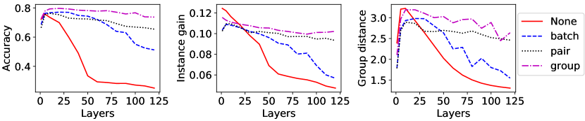
Figure 1: The test accuracy, instance information gain, and group distance ratio of SGC on Cora. We compare differentiable group normalization with none, batch and pair normalizations.

Based on the two proposed metrics, we take simple graph convolution networks (SGC) as an example, and analyze the over-smoothing issue on Cora dataset [25]. SGC simplifies the model through removing all the trainable weights between layers to avoid the potential of overfitting [12]. So the over-smoothing issue would be the major cause of performance dropping in SGC. As shown by the red lines in Figure 1, the graph convolutions first exploit neighborhood information to improve test accuracy up to $K=5$, after which the over-smoothing issue starts to worsen the performance. At the same time, instance information gain $G_{\mathrm{Ins}}$ and group distance ratio $R_{\mathrm{Group}}$ decrease due to the over-smoothing issue. For the extreme case of $K=120$, the input features are filtered out and all groups of nodes converge to the same representation vector, leading to $G_{\mathrm{Ins}}=0$ and $R_{\mathrm{Group}}=1$, respectively. Our metrics quantify the smoothness of node representations based on group structures, but also have the similar variation tendency with test accuracy to indicate it well.

3 Differentiable Group Normalization

We start with a graph-regularized optimization problem [10, 19]. To optimize the over-smoothing metrics of $G_{\mathrm{Ins}}$ and $R_{\mathrm{Group}}$, one traditional approach is to minimize the loss function:

$$\mathcal{L}=\mathcal{L}_{0}-G_{\mathrm{Ins}}-\lambda R_{\mathrm{Group}}.$$ (4)

$\mathcal{L}_{0}$ denotes the supervised cross-entropy loss w.r.t. representation probability vectors $h_{v}\in\mathbb{R}^{C\times 1}$ and class labels. $\lambda$ is a balancing factor. The goal of optimization problem Eq. (4) is to learn node representations close to the input features and informative for their class labels. Considering the labeled graph communities, it also improves the intra-group similarity and inter-group distance. However, it is non-trivial to optimize this objective function due to the non-derivative of non-parametric statistic $G_{\mathrm{Ins}}$ [29, 30] and the expensive computation of $R_{\mathrm{Group}}$.

3.1 Proposed Technique for Addressing Over-smoothing

Instead of directly optimizing regularized problem in Eq. (4), we propose the differentiable group normalization (DGN) applied between graph convolutional layers to normalize the node embeddings group by group. The key intuition is to cluster nodes into multiple groups and then normalize them independently. Consider the labeled node groups (or communities) in networked data. The node embeddings within each group are expected to be rescaled with a specific mean and variance to make them similar. Meanwhile, the embedding distributions from different groups are separated by adjusting their means and variances. We develop an analogue with the group normalization in convolutional neural networks (CNNs) [26], which clusters a set of adjacent channels with similar characteristics into a group and treats it independently. Compared with standard CNNs, the challenge in designing DGN is how to cluster nodes in a suitable way. The clustering needs to be in line with the embedding and labels, during the dynamic learning process.

We address this challenge by learning a cluster assignment matrix, which softly maps nodes with close embeddings into a group. Under the supervision of training labels, the nodes close in the embedding space tend to share a common label. To be specific, we first describe how DGN clusters and normalizes nodes in a group-wise fashion given an assignment matrix. After that, we discuss how to learn the assignment matrix to support differentiable node clustering.

Group Normalization. Let $H^{(k)}=[h_{1}^{(k)},\cdots,h_{n}^{(k)}]^{T}\in\mathbb{R}^{n\times d^{(k)}}$ denote the embedding matrix generated from the $k$-th graph convolutional layer. Taking $H^{(k)}$ as input, DGN softly assigns nodes into groups and normalizes them independently to output a new embedding matrix for the next layer. Formally, we define the number of groups as $G$, and denote the cluster assignment matrix by $S^{(k)}\in\mathbb{R}^{n\times G}$. $G$ is a hyperparameter that could be tuned per dataset. The $i$-th column of $S^{(k)}$, i.e., $S^{(k)}[:,i]$, indicates the assignment probabilities of nodes in a graph to the $i$-th group. Supposing that $S^{(k)}$ has already been computed, we cluster and normalize nodes in each group as follows:

$$H^{(k)}_{i}=S^{(k)}[:,i]\circ H^{(k)}\in\mathbb{R}^{n\times d^{(k)}};\quad\tilde{H}^{(k)}_{i}=\gamma_{i}(\frac{H^{(k)}_{i}-\mu_{i}}{\sigma_{i}})+\beta_{i}\in\mathbb{R}^{n\times d^{(k)}}.$$ (5)

Symbol $\circ$ denotes the row-wise multiplication. The left part in the above equation represents the soft node clustering for group $i$, whose embedding matrix is given by $H^{(k)}_{i}$. The right part performs the standard normalization operation. In particular, $\mu_{i}$ and $\sigma_{i}$ denote the vectors of running mean and standard deviation of group $i$, respectively, and $\gamma_{i}$ and $\beta_{i}$ denote the trainable scale and shift vectors, respectively. Given the input embedding $H^{(k)}$ and the series of normalized embeddings $\{\tilde{H}^{(k)}_{1},\cdots,\tilde{H}^{(k)}_{G}\}$, DGN generates the final embedding matrix $\tilde{H}^{(k)}$ for the next layer as follows:

$$\tilde{H}^{(k)}=H^{(k)}+\lambda\sum_{i=1}^{G}\tilde{H}^{(k)}_{i}\in\mathbb{R}^{n\times d^{(k)}}.$$ (6)

$\lambda$ is a balancing factor as mentioned before. Inspecting the loss function in Eq. (4), DGN utilizes components $H^{(k)}$ and $\sum_{i=1}^{G}\tilde{H}^{(k)}_{i}$ to improve terms $G_{\mathrm{Ins}}$ and $R_{\mathrm{Group}}$, respectively. In particular, we preserve the input embedding $H^{(k)}$ to avoid over-normalization and keep the input feature of each node to some extent. Note that the linear combination of $H^{(k)}$ in DGN is different from the skip connection in GNN models [31, 32], which instead connects the embedding output $H^{(k-1)}$ from the last layer. The technique of skip connection could be included to further boost the model performance. Group normalization $\sum_{i=1}^{G}\tilde{H}^{(k)}_{i}$ rescales the node embeddings within each group independently to make them similar. Ideally, we assign the close node embeddings with a common label to a group. Node embeddings of the group are then distributed closely around the corresponding running mean. Thus for different groups associate with distinct node labels, we disentangle their running means and separates the node embedding distributions. By applying DGN between the successive graph convolutional layers, we are able to optimize Problem (4) to mitigate the over-smoothing issue.

Differentiable Clustering. We apply a linear model to compute the cluster assignment matrix $S^{(k)}$ used in Eq. (5). The mathematical expression is given by:

$$S^{(k)}=\mathrm{softmax}(H^{(k)}U^{(k)}).$$ (7)

$U^{(k)}\in\mathbb{R}^{d^{(k)}\times G}$ denotes the trainable weights for a DGN module applied after the $k$-th graph convolutional layer. $\mathrm{softmax}$ function is applied in a row-wise way to produce the normalized probability vector w.r.t all the $G$ groups for each node. Through the inner product between $H^{(k)}$ and $U^{(k)}$, the nodes with close embeddings are assigned to the same group with a high probability. Here we give a simple and effective way to compute $S^{(k)}$. Advanced neural networks could be applied.

Time Complexity Analysis. Suppose that the time complexity of embedding normalization at each group is $\mathcal{O}(T)$, where $T$ is a constant depending on embedding dimension $d^{(k)}$ and node number $n$. The time cost of group normalization $\sum_{i=1}^{G}\tilde{H}^{(k)}_{i}$ is $\mathcal{O}(GT)$. Both the differentiable clustering (in Eq. (5)) and the linear model (in Eq. (7)) have a time cost of $\mathcal{O}(nd^{(k)}G)$. Thus the total time complexity of a DGN layer is given by $\mathcal{O}(nd^{(k)}G+GT)$, which linearly increases with $G$.

Comparison with Prior Work. To the best of our knowledge, the existing work mainly focuses on analyzing and improving the node pair distance to relieve the over-smoothing issue [19, 21, 24]. One of the general solutions is to train GNN models regularized by the pair distance [19]. Recently, there are two related studies applying batch normalization [22] or pair normalization [24] to keep the overall pair distance in a graph. Pair normalization is a “slim” realization of batch normalization by removing the trainable scale and shift. However, the metric of pair distance and the resulting techniques ignore global graph structure, and may achieve sub-optimal performance in practice. In this work, we measure over-smoothing of GNN models based on communities/groups and independent node instances. We then formulate the problem in Eq. (4) to optimize the proposed metrics, and propose DGN to solve it in an efficient way, which in turn addresses the over-smoothing issue.

3.2 Evaluating Differentiable Group Normalization on Attributed Graphs

We apply DGN to the SGC model to validate its effectiveness in relieving the over-smoothing issue. Furthermore, we compare with the other two available normalization techniques used upon GNNs, i.e., batch normalization and pair normalization. As shown in Figure 1, the test accuracy of DGN remains stable with the increase in the number of layers. By preserving the input embedding and normalizing node groups independently, DGN achieves superior performance in terms of instance information gain as well as group distance ratio. The promising results indicate that our DGN tackles the over-smoothing issue more effectively, compared with none, batch and pair normalizations.

It should be noted that, the highest accuracy of $79.7\%$ is achieved with DGN when $K=20$. This observation contradicts with the common belief that GNN models work best with a few layers on current benchmark datasets [33]. With the integration of advanced techniques, such as DGN, we are able to exploit deeper GNN architectures to unleash the power of deep learning in network analysis.

3.3 Evaluation in Scenario with Missing Features

To further illustrate that DGN could enable us to achieve better performance with deeper GNN architectures, we apply it to a more complex scenario. We assume that the attributes of nodes in the test set are missing. It is a common scenario in practice [24]. For example, in social networks, new users are often lack of profiles and tags [34]. To perform prediction tasks on new users, we would rely on the node attributes of existing users and their connections to new users. In such a scenario, we would like to apply more layers to exploit the neighborhood structure many hops away to improve node representation learning. Since the over-smoothing issue gets worse with the increasing of layer numbers, the benefit of applying normalization will be more obvious in this scenario.

We remove the input features of both validation and test sets in Cora, and replace them with zeros [24]. Figure 2 presents the results on three widely-used models, i.e., SGC, graph convolutional networks (GCN), and graph attention networks (GAT). Due to the over-smoothing issue, GNN models without any normalization fail to distinguish nodes quickly with the increasing number of layers. In contrast, the normalization techniques reach their highest performance at larger layer numbers, after which they drop slowly. We observe that DGN obtains the best performance with $50$, $20$, and $8$ layers for SGC, GCN, and GAT, respectively. These layer numbers are significantly larger than those of the widely-used shallow models (e.g., two or three layers).

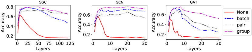
Figure 2: The test accuracies of SGC, GCN, and GAT models on Cora with missing features. We compare differentiable group normalization with none, batch and pair normalizations.

4 Experiments

We now empirically evaluate the effectiveness and robustness of DGN on real-world datasets. We aim to answer three questions as follows. Q1: Compared with the state-of-the-art normalization methods, can DGN alleviate the over-smoothing issue in GNNs in a better way? Q2: Can DGN help GNN models achieve better performance by enabling deeper GNNs? Q3: How do the hyperparameters influence the performance of DGN?

4.1 Experiment Setup

Datasets. Joining the practice of previous work, we evaluate GNN models by performing the node classification task on four datasets: Cora, Citeseer, Pubmed [25], and CoauthorCS [35]. We also create graphs by removing features in validation and test sets. The dataset statistics are in Appendix.

Implementations. Following the previous settings, we choose the hyperparameters of GNN models and optimizer as follows. We set the number of hidden units to $16$ for GCN and GAT models. The number of attention heads in GAT is $1$. Since a larger parameter size in GCN and GAT may lead to overfitting and affects the study of over-smoothing issue, we compare normalization methods by varying the number of layers $K$ in $\{1,2,\cdots,10,15,\cdots,30\}$. For SGC, we increase the testing range and vary $K$ in $\{1,5,10,20,\cdots,120\}$. We train with a maximum of $1000$ epochs using the Adam optimizer [36] and early stopping. Weights in GNN models are initialized with Glorot algorithm [37]. We use the following sets of hyperparameters for Citeseer, Cora, CoauthorCS: $0.6$ (dropout rate), $5\cdot 10^{-4}$ (L2 regularization), $5\cdot 10^{-3}$ (learning rate), and for Pubmed: $0.6$ (dropout rate), $1\cdot 10^{-3}$ (L2 regularization), $1\cdot 10^{-2}$ (learning rate). We run each experiment $5$ times and report the average.

Baselines. We compare with none normalization (NN), batch normalization (BN) [22, 23] and pair normalization (PN) [24]. Their technical details are listed in Appendix.

DGN Configurations. The key hyperparameters include group number $G$ and balancing factor $\lambda$. Depending on the number of class labels, we apply $5$ groups to Pubmed and $10$ groups to the others. The criterion is to use more groups to separate representation distributions in networked data accompanied with more class labels. $\lambda$ is tuned on validation sets to find a good trade-off between preserving input features and group normalization. We introduce the selection of $\lambda$ in Appendix.

4.2 Experiment Results

Studies on alleviating the over-smoothing problem. To answer Q1, Table 1 summarizes the results of applying different normalization techniques to GNN models on all datasets. We report the performance of GCN and GAT with $2/15/30$ layers, and SGC with $5/60/120$ layers due to space limit. We provide test accuracies, instance information gain and group distance ratio under all depths in Appendix. It can be observed that DGN has significantly alleviated the over-smoothing issue. Given the same layers, DGN almost outperforms all other normalization methods for all cases and greatly slows down the performance dropping. It is because the self-preserved component $H^{(k)}$ in Eq. (6) keeps the informative input features and avoids over-normalization to distinguish different nodes. This component is especially crucial for models with a few layers since the over-smoothing issue has not appeared. The other group normalization component in Eq. (6) processes each group of nodes independently. It disentangles the representation similarity between groups, and hence reduces the over-smoothness of nodes over a graph accompanied with graph convolutions.

Table 1: Test accuracy in percentage on attributed networks. Layers $a/b$ denote the layer number $a$ in GCN & GAT and that of $b$ in SGC. $\#K$ denotes the optimal layer numbers where DGN achieves the highest performance.

Dataset	Model	Layers 2/5				Layers 15/60				Layers 30/120				#K
		NN	BN	PN	DGN	NN	BN	PN	DGN	NN	BN	PN	DGN
Cora	GCN	$\bm{82.2}$	$73.9$	$71.0$	$82.0$	$18.1$	$70.3$	$67.2$	$\bm{75.2}$	$13.1$	$67.2$	$64.3$	$\bm{73.2}$	$2$
	GAT	$80.9$	$77.8$	$74.4$	$\bm{81.1}$	$16.8$	$33.1$	$49.6$	$\bm{71.8}$	$13.0$	$25.0$	$30.2$	$\bm{51.3}$	$2$
	SGC	$75.8$	$76.3$	$75.4$	$\bm{77.9}$	$29.4$	$72.1$	$71.7$	$\bm{77.8}$	$25.1$	$51.2$	$65.5$	$\bm{73.7}$	$20$
Citeseer	GCN	$\bm{70.6}$	$51.3$	$60.5$	$69.5$	$15.2$	$46.9$	$46.7$	$\bm{53.1}$	$9.4$	$47.9$	$47.1$	$\bm{52.6}$	$2$
	GAT	$\bm{70.2}$	$61.5$	$62.0$	$69.3$	$22.6$	$28.0$	$41.4$	$\bm{52.6}$	$7.7$	$21.4$	$33.3$	$\bm{45.6}$	$2$
	SGC	$\bm{69.6}$	$58.8$	$64.8$	$69.5$	$\bm{66.3}$	$50.5$	$65.0$	$63.4$	$60.8$	$47.3$	$63.1$	$\bm{64.7}$	$30$
Pubmed	GCN	$79.3$	$74.9$	$71.1$	$\bm{79.5}$	$22.5$	$73.7$	$70.6$	$\bm{76.1}$	$18.0$	$70.4$	$70.4$	$\bm{76.9}$	$2$
	GAT	$\bm{77.8}$	$76.2$	$72.4$	$77.5$	$37.5$	$56.2$	$68.8$	$\bm{75.9}$	$18.0$	$46.6$	$58.2$	$\bm{73.3}$	$5$
	SGC	$71.5$	$76.5$	$75.8$	$\bm{76.8}$	$34.2$	$75.2$	$77.1$	$\bm{77.4}$	$23.1$	$71.6$	$76.7$	$\bm{77.1}$	$10$
Coauthors	GCN	$92.3$	$86.0$	$77.8$	$\bm{92.3}$	$72.2$	$78.5$	$69.5$	$\bm{83.7}$	$3.3$	$\bm{84.7}$	$64.5$	$84.4$	$1$
	GAT	$91.5$	$89.4$	$85.9$	$\bm{91.8}$	$6.0$	$77.7$	$53.1$	$\bm{84.5}$	$3.3$	$16.7$	$48.1$	$\bm{75.5}$	$1$
	SGC	$89.9$	$88.7$	$86.0$	$\bm{90.2}$	$10.2$	$59.7$	$76.4$	$\bm{81.3}$	$5.8$	$30.5$	$52.6$	$\bm{60.8}$	$1$

Studies on enabling deeper and better GNNs. To answer Q2, we compare all of the concerned normalization methods over GCN, GAT, and SGC in the scenario with missing features. As we have discussed, normalization techniques will show their power in relieving the over-smoothing issue and exploring deeper architectures especially for this scenario. In Table 2, Acc represents the best test accuracy yielded by model equipped with the optimal layer number $\#K$. We can observe that DGN significantly outperforms the other normalization methods on all cases. The average improvements over NN, BN and PN achieved by DGN are $37.8\%$, $7.1\%$ and $12.8\%$, respectively. Compared with vanilla GNN models without any normalization layer, the optimal models accompanied with normalization layers (especially for our DGN) usually possess larger values of $\#K$. It demonstrates that DGN enables to explore deeper architectures to exploit neighborhood information with more hops away by tackling the over-smoothing issue. We present the comprehensive analyses in terms of test accuracy, instance information gain and group distance ratio under all depths in Appendix.

Table 2: The highest accuracy (%) and the accompanied optimal layers in the scenario with missing features. We calculate the average improvement achieved by DGN over each GNN framework.

Model	Norm	Cora		Citeseer		Pubmed		CoauthorCS		Improvement%
		Acc	#K	Acc	#K	Acc	#K	Acc	#K
GCN	NN	$57.3$	$3$	$44.0$	$6$	$36.4$	$4$	$67.3$	$3$	$42.2$
	BN	$71.8$	$20$	$45.1$	$25$	$70.4$	$30$	$82.7$	$30$	$5.2$
	PN	$65.6$	$20$	$43.6$	$25$	$63.1$	$30$	$63.5$	$4$	$19.2$
	DGN	$\bm{76.3}$	$\bm{20}$	$\bm{50.2}$	$\bm{30}$	$\bm{72.0}$	$\bm{30}$	$\bm{83.7}$	$\bm{25}$	-
GAT	NN	$50.1$	$2$	$40.8$	$4$	$38.5$	$4$	$63.7$	$3$	$51.0$
	BN	$72.7$	$5$	$48.7$	$5$	$60.7$	$4$	$80.5$	$6$	$9.8$
	PN	$68.8$	$8$	$50.3$	$6$	$63.2$	$20$	$66.6$	$3$	$14.7$
	DGN	$\bm{75.8}$	$\bm{8}$	$\bm{54.5}$	$\bm{5}$	$\bm{72.3}$	$\bm{20}$	$\bm{83.6}$	$\bm{15}$	-
SGC	NN	$63.4$	$5$	$51.2$	$40$	$63.7$	$5$	$71.0$	$5$	$20.1$
	BN	$78.5$	$20$	$50.4$	$20$	$72.3$	$50$	$84.4$	$20$	$6.2$
	PN	$73.4$	$50$	$58.0$	$120$	$75.2$	$30$	$80.1$	$10$	$4.5$
	DGN	$\bm{80.2}$	$\bm{50}$	$\bm{58.2}$	$\bm{90}$	$\bm{76.2}$	$\bm{90}$	$\bm{85.8}$	$\bm{20}$	-

Hyperparameter studies. We study the impact of hyperparameters, group number $G$ and balancing factor $\lambda$, on DGN in order to answer research question Q3. Over the GCN framework associated with $20$ convolutional layers, we evaluate DGN by considering $G$ and $\lambda$ from sets $[1,5,10,15,20,30]$ and $[0.001,0.005,0.01,0.03,0.05,0.1]$, respectively. The left part in Figure 3 presents the test accuracy for each hyperparameter combination. We observe that: (i) The model performance is damaged greatly when $\lambda$ is close to zero (e.g., $\lambda=0.001$). In this case, group normalization contributes slightly in DGN, resulting in over-smoothing in the GCN model. (ii) Model performance is not sensitive to the value of $G$, and an appropriate $\lambda$ value could be tuned to optimize the trade-off between instance gain and group normalization. It is because DGN learns to use the appropriate number of groups by end-to-end training. In particular, some groups might not be used as shown in the right part of Figure 3, at which only $6$ out of $10$ groups (denoted by black triangles) are adopted. (iii) Even when $G=1$, DGN still outperforms BN by utilizing the self-preserved component to achieve an accuracy of $74.7\%$, where $\lambda=0.1$. Via increasing the group number, the model performance could be further improved, e.g., the accuracy of $76.3\%$ where $G=10$ and $\lambda=0.01$.

Node representation visualization. We investigate how DGN clusters nodes into different groups to tackle the over-smoothing issue. The middle and right parts of Figure 3 visualize the node representations achieved by GCN models without normalization tool and with the DGN approach, respectively. It is observed that the node representations of different classes mix together when the layer number reaches $20$ in the GCN model without normalization. In contrast, our DGN method softly assigns nodes into a series of groups, whose running means at the corresponding normalization modules are highlighted with black triangles. Through normalizing each group independently, the running means are separated to improve inter-group distances and disentangle node representations. In particular, we notice that the running means locate at the borders among different classes (e.g., the upper-right triangle at the border between red and pink classes). That is because the soft assignment may cluster nodes of two or three classes into the same group. Compared with batch or pair normalization, the independent normalization for each group only includes a few classes in DGN. In this way, we relieve the representation noise from other node classes during normalization, and improve the group distance ratio as illustrated in Appendix.

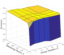
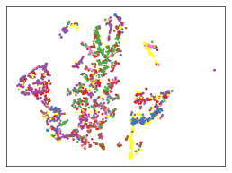
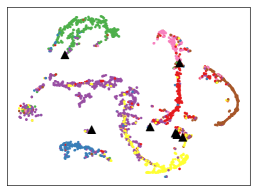
Figure 3: Left: Test accuracies of GCN with $20$ layers on Cora with missing features, where hyperparameters $G$ and $\lambda$ are studied. Middle: Node representation visualization for GCN without normalization and with $K=20$. Right: Node representation visualization for GCN with DGN layer and $K=20$ (node colors represent classes, and black triangles denote the running means of groups).

5 Conclusion

In this paper, we propose two over-smoothing metrics based on graph structures, i.e., group distance ratio and instance information gain. By inspecting GNN models through the lens of these two metrics, we present a novel normalization layer, DGN, to boost model performance against over-smoothing. It normalizes each group of similar nodes independently to separate node representations of different classes. Experiments on real-world classification tasks show that DGN greatly slowed down performance degradation by alleviating the over-smoothing issue. DGN enables us to explore deeper GNNs and achieve higher performance in analyzing attributed networks and the scenario with missing features. Our research will facilitate deep learning models for potential graph applications.

Broader Impact

The successful outcome of this work will lead to advances in building up deep graph neural networks and dealing with complex graph-structured data. The developed metrics and algorithms have an immediate and strong impact on a number of fields, including (1) Over-smoothing Quantitative Analysis: GNN models tend to result in the over-smoothing issue with the increase in the number of layers. During the practical development of deeper GNN models, the proposed instance information gain and group distance ratio effectively indicate the over-smoothing issue, in order to push the model exploration toward a good direction. (2) Deep GNN Modeling: The proposed differentiable group normalization tool successfully tackles the over-smoothing issue and enables the modeling of deeper GNN variants. It encourages us to fully unleash the power of deep learning in processing the networked data. (3) Real-world Network Analytics Applications: The proposed research will broadly shed light on utilizing deep GNN models in various applications, such as social network analysis, brain network analysis, and e-commerce network analysis. For such complex graph-structured data, deep GNN models can exploit the multi-hop neighborhood information to boost the task performance.

Appendix A Dataset Statistics

For fair comparison with previous work, we perform the node classification task on four benchmark datasets, including Cora, Citeseer, Pubmed [25], and CoauthorCS [35]. They have been widely adopted to study the over-smoothing issue in GNNs [21, 19, 24, 16, 20]. The detailed statistics are listed in Table 3. To further illustrate that the normalization techniques could enable deeper GNNs to achieve better performance, we apply them to a more complex scenario with missing features. For these four benchmark datasets, we create the corresponding scenarios by removing node features in both validation and testing sets.

Table 3: Dataset statistics on Cora, Citeseer, Pubmed, and CoauthorCS.

	Cora	Citeseer	Pubmed	CoauthorCS
#Nodes	$2708$	$3327$	$19717$	$18333$
#Edges	$5429$	$4732$	$44338$	$81894$
#Features	$1433$	$3703$	$500$	$6805$
#Classes	$7$	$6$	$3$	$15$
#Training Nodes	$140$	$120$	$60$	$600$
#Validation Nodes	$500$	$500$	$500$	$2250$
#Testing Nodes	$1000$	$1000$	$1000$	$15483$

Appendix B Running Environment

All the GNN models and normalization approaches are implemented in PyTorch, and tested on a machine with 24 Intel(R) Xeon(R) CPU E5-2650 v4 @ 2.20GB processors, GeForce GTX-1080 Ti 12 GB GPU, and 128GB memory size. We implement the group normalization in a parallel way. Thus the practical time cost of our DGN is comparable to that of traditional batch normalization.

Appendix C GNN Models

We test over three general GNN models to illustrate the over-smoothing issue, including graph convolutional networks (GCN) [10], graph attention networks (GAT) [11] and simple graph convolution (SGC) networks [12]. We list their neighbor aggregation functions in Table 4.

Table 4: Neighbor aggregation function at a graph convolutional layer for GCN, GAT and SGC.

Model	Neighbor aggregation function
GCN	$h^{(k)}_{v}=\mathrm{ReLU}(\sum_{v^{\prime}\in\mathcal{N}(v)\cup\{v\}}\frac{1}{\sqrt{(|\mathcal{N}(v)|+1)\cdot(|\mathcal{N}(v^{\prime})|+1)}}W^{(k)}h_{v^{\prime}}^{(k-1)})$
GAT	$h^{(k)}_{v}=\mathrm{ReLU}(\sum_{v^{\prime}\in\mathcal{N}(v)\cup\{v\}}a_{vv^{\prime}}^{(k)}W^{(k)}h_{v^{\prime}}^{(k-1)})$
SGC	$h^{(k)}_{v}=\sum_{v^{\prime}\in\mathcal{N}(v)\cup\{v\}}\frac{1}{\sqrt{(|\mathcal{N}(v)|+1)\cdot(|\mathcal{N}(v^{\prime})|+1)}}h_{v^{\prime}}^{(k-1)}$

Considering the message passing strategy as shown by Eq. (1) in the main manuscript, we explain the key properties of GCN, GAT and SGC as follows. GCN merges the information from node itself and its neighbors weighted by vertices’ degrees, where $a^{(k)}_{vv^{\prime}}=1./\sqrt{(|\mathcal{N}(v)|+1)\cdot(|\mathcal{N}(v^{\prime})|+1)}$. Functions $\mathrm{AGG}$ and $\mathrm{COM}$ are realized by a summation pooling. The activation function of ReLU is then applied to non-linearly transform the latent embedding. Based on GCN, GAT uses an additional attention layer to learn link weight $a^{(k)}_{vv^{\prime}}$. GAT aggregates neighbors with the trainable link weights, and achieves significant improvements in a variety of applications. SGC is simplified from GCN by removing all trainable parameters $W^{(k)}$ and nonlinear activations between successive layers. It has been empirically shown that these simplifications do not negatively impact classification accuracy, and even relive the problems of over-fitting and vanishing gradients in deeper models.

Appendix D Normalization Baselines

Batch normalization is first applied between the successive convolutional layers in CNNs [23]. It is extended to graph neural networks to improve node representation learning and generalization [22]. Taking embedding matrix $H^{(k)}$ as input after each layer, batch normalization scales the node representations using running mean and variance, and generates a new embedding matrix for the next graph convolutional layer. Formally, we have:

$$\tilde{H}^{(k)}=\gamma(\frac{H^{(k)}-\mu}{\sigma})+\beta\in\mathbb{R}^{n\times d^{(k)}}.$$

$\mu$ and $\sigma$ denote the vectors of running mean and standard deviation, respectively; $\gamma$ and $\beta$ denote the trainable scale and shift vectors, respectively. Recently, pair normalization has been proposed to tackle the over-smoothing issue in GNNs, targeting at maintaining the average node pair distance over a graph [24]. Pair normalization is a simplifying realization of batch normalization by removing the trainable $\gamma$ and $\beta$. In this work, we augment each graph convolutional layer via appending a normalization module, in order to validate the effectiveness of normalization technique in relieving over-smoothing and enabling deeper GNNs.

Appendix E Hyperparameter Tuning in DGN

The balancing factor, $\lambda$, is crucial to determine the trade-off between input feature preservation and group normalization in DGN. It needs to be tuned carefully as GNN models increase the number of layers. To be specific, we consider the candidate set $\{5\cdot 10^{-4},1\cdot 10^{-3},2\cdot 10^{-3},3\cdot 10^{-3},5\cdot 10^{-3},1\cdot 10^{-2},2\cdot 10^{-2},3\cdot 10^{-2},5\cdot 10^{-2}\}$. For each specific model, we use a few epochs to choose the optimal $\lambda$ on the validation set, and then evaluate it on the testing set. We observe that the value of $\lambda$ tends to be larger in the model accompanied with more graph convolutional layers. That is because the over-smoothing issue gets worse with the increase in layer number. The group normalization is much more required to separate the node representations of different classes.

Appendix F Instance Information Gain

In this work, we adopt kernel-density estimators (KDE), one of the common non-parametric approaches, to estimate the mutual information between input feature and representation vector [29, 30]. A key assumption in KDE is that the input feature (or output representation vector) of neural networks is distributed as a mixture of Gaussians. Since a neural network is a deterministic function of the input feature after training, the mutual information would be infinite without such assumption. In the following, we first formally define the Gaussian assumption, input probability distribution and representation probability distribution, and then present how to obtain the instance information gain based on the mutual information metric.

Gaussian assumption.

In the graph signal processing, it is common to assume that the collected input feature contains both true signal and noise. In other word, we have the input feature as follows: $x_{v}=\bar{x}_{v}+\epsilon_{x}$. $\bar{x}_{v}$ denotes the true value, and $\epsilon_{x}\sim\mathcal{N}(0,\sigma^{2}\bm{I})$ denotes the added Gaussian noise with variance $\sigma^{2}$. Therefore, input feature $x_{v}$ is a Gaussian variable centered on its true value.

Input probability distribution.

We treat the empirical distribution of input samples as true distribution. Given a dataset accompanied with $n$ samples, we have a series of input features $\{x_{1},\cdots,x_{n}\}$ for all the samples. Each node feature is sampled with probability $1/|\mathcal{V}|$ following the empirical uniform distribution. Let $|\mathcal{V}|$ denotes the number of samples, and let $\mathcal{X}$ denote the random variable of input features. Based on the above Gaussian assumption, probability $P_{\mathcal{X}}(x_{v})$ of input feature $x_{v}$ is obtained by the product of $1/|\mathcal{V}|$ with Gaussian probability centered on true value $\bar{x}_{v}$.

Representation probability distribution.

Let $\mathcal{H}$ denote the random variable of node representations. To obtain probability $P_{\mathcal{H}}(h_{v})$ of continuous vector $h_{v}$, a general approach is to bin and transform $\mathcal{H}$ into a new discrete variable. However, with the increasing dimensions of $h_{v}$, it is non-trivial to statistically count the frequencies of all possible discrete values. Considering the task of node classification, the index of largest element along vector $h_{v}\in\mathbb{R}^{C\times 1}$ is regarded as the label of a node. We propose a new binning approach that labels the whole vector $h_{v}$ with the largest index $z_{v}$. In this way, we only have $C$ classes of discrete values to facilitate the frequency counting. To be specific, let $\bf P_{c}$ denote the number of representation vectors whose indexes $z_{v}=c$. The probability of a discrete variable with class $c$ is given by: $p_{c}=P_{\mathcal{H}}(z_{v}=c)=\frac{\bf P_{c}}{\sum_{l=1}^{C}\bf P_{l}}$.

Mutual information calculation.

Based on KDE approach, a lower bound of mutual information between input feature and representation vector can be calculated as:

$$\begin{array}[]{rl}G_{\mathrm{Ins}}=I(\mathcal{X};\mathcal{H})&=\sum_{x_{v}\in\mathcal{X},h_{v}\in\mathcal{H}}P_{\mathcal{XH}}(x_{v},h_{v})\log\frac{P_{\mathcal{XH}}(x_{v},h_{v})}{P_{\mathcal{X}}(x_{v})P_{\mathcal{H}}(h_{v})}\\ \\ &=H({\mathcal{X}})-H({\mathcal{X}}|{\mathcal{H}})\\ \\ &\geq-\frac{1}{|\mathcal{V}|}\sum_{i}\log{\frac{1}{|\mathcal{V}|}}\sum_{j}\exp(-\frac{1}{2}\frac{||x_{i}-x_{j}||_{2}^{2}}{4\sigma^{2}})\\ &\quad-\sum_{c=1}^{C}p_{c}[-\frac{1}{\bf P_{c}}\sum_{i,z_{i}=c}\log{\frac{1}{\bf P_{c}}}\sum_{j,z_{j}=c}\exp(-\frac{1}{2}\frac{||x_{i}-x_{j}||_{2}^{2}}{4\sigma^{2}})].\end{array}$$

The sum over $i,z_{i}=c$ represents a summation over all the input features whose representation vectors are labeled with $z_{i}=c$. $P_{\mathcal{XH}}(x_{v},h_{v})$ denotes the joint probability of $x_{v}$ and $h_{v}$. The effectiveness of $G_{\mathrm{Ins}}$ in measuring mutual information between input feature and node representation has been demonstrated in the experimental results. As illustrated in Figures 5-7, $G_{\mathrm{Ins}}$ decreases with the increasing number of graph convolutional layers. This practical observation is in line with the human expert knowledge about neighbor aggregation strategy in GNNs. The neighbor aggregation function as shown in Table 4 is in fact a low-passing smoothing operation, which mixes the input feature of a node with those of its neighbors gradually. At the extreme cases where $K=30$ or $120$, we find that $G_{\mathrm{Ins}}$ approaches to zero in GNN models without normalization. The loss of informative input feature leads to the dropping of node classification accuracy. However, our DGN keeps the input information during graph convolutions and normalization to some extent, resulting in the largest $G_{\mathrm{Ins}}$ compared with the other normalization approaches.

Appendix G Performance Comparison on Attributed Graphs

In this section, we report the model performances in terms of test accuracy, instance information gain and group distance ratio achieved on all the concerned datasets in Figures 5-7. We make the following observations:

• Comparing with other normalization techniques, our DGN generally slows down the dropping of test accuracy with the increase in layer number. Even for GNN models associated with a small number of layers (i.e., $G\leq 5$), DGN achieves the competitive performance compared with none normalization. The adoption of DGN module does not damage the model performance, and prevents model from suffering over-smoothing issue when GNN goes deeper.

• DGN achieves the larger or comparable instance information gains in all cases, especially for GAT models. That is because DGN keeps embedding matrix $H^{(k)}$ and prevents over-normalization within each group. The preservation of $H^{(k)}$ saves input features to some extent after each layer of graph convolutions and normalization. In an attributed graph, the improved preservation of informative input features in the final representations will significantly facilitate the downstream node classification. Furthermore, such preservation is especially crucial for GNN models with a few layers, since the over-smoothing issue has not appeared.

• DGN normalizes each group of node representations independently to generally improve the group distance ratio, especially for models GCN and GAT. A larger value of group distance ratio means that the node representation distributions from all groups are disentangled to address the over-smoothing issue. Although the ratios of DGN are smaller than those of pair normalization in some cases upon SGC framework, we still achieve the largest test accuracy. That may be because the intra-group distance in DGN is much smaller than that of pair normalization. A small value of intra-group distance would facilitate the node classification within the same group. We will further compare the intra-group distance in scenarios with missing features in the following experiments.

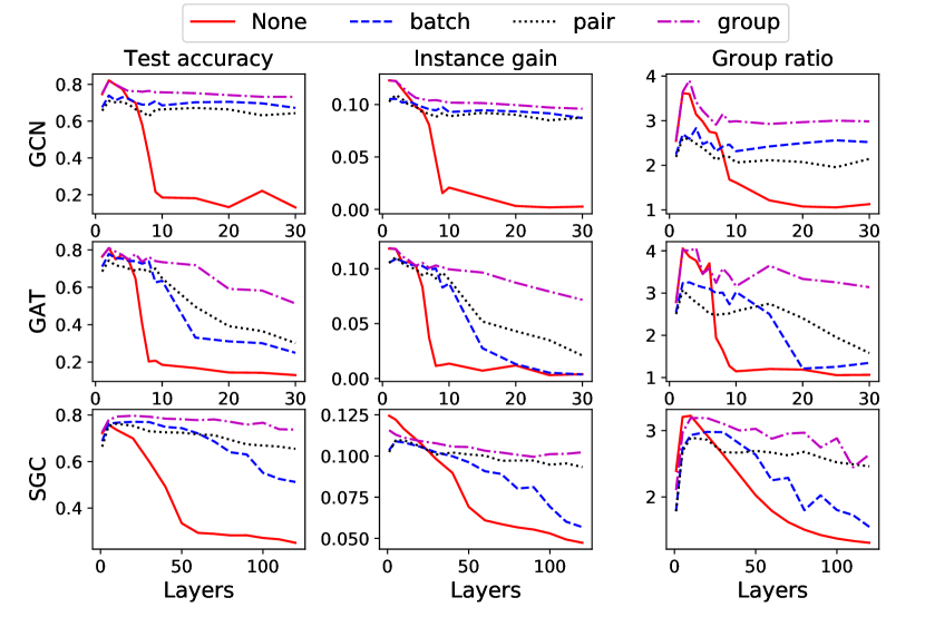
Figure 4: The test accuracy, instance information gain, and group distance ratio in attributed Cora. We compare differentiable group normalization with none, batch and pair normalizations.

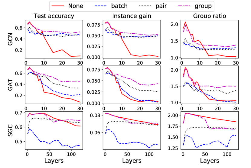
Figure 5: The test accuracy, instance information gain, and group distance ratio in attributed Citeseer. We compare differentiable group normalization with none, batch and pair normalizations.

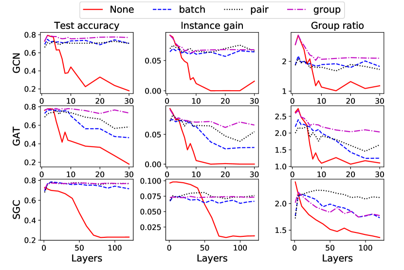
Figure 6: The test accuracy, instance information gain, and group distance ratio in attributed Pubmed. We compare differentiable group normalization with none, batch and pair normalizations.

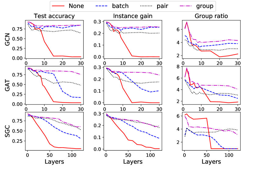
Figure 7: The test accuracy, instance information gain, and group distance ratio in attributed CoauthorCS. We compare differentiable group normalization with none, batch and pair normalizations.

Appendix H Performance Comparison in Scenarios with Missing Features

In this section, we report the model performances in terms of test accuracy, group distance ratio and intra-group distance achieved in scenarios with missing features in Figures 9-11. The intra-group distance is calculated by node pair distance averaged within the same group. Its mathematical expression is given by the denominator of Equation (3) in the main manuscript. We make the following observations:

• DGN achieves the largest test accuracy by exploring the deeper neural architecture with a larger number of graph convolutional layers. In the scenarios with missing features, GNN model relies highly on the neighborhood structure to classify nodes. DGN enables the deeper GNN model to exploit neighborhood structure with multiple hops away, and at the same time relieves the over-smoothing issue.

• Comparing with other normalization techniques, DGN generally improves the group distance ratio to relieve over-smoothing issue. Although in some cases the ratios are smaller than those of pair normalization upon SGC framework, we still achieve the comparable or even better test accuracy. That is because DGN has a smaller intra-group distance to facilitate node classification within the same group, which is analyzed in the followings.

• DGN obtains an appropriate intra-group distance to optimize the node classification task. While the over-smoothing issue results in an extremely-small distance in the model without normalization, a larger one in pair normalization leads to the inaccurate node classification within each group. That is because the pair normalization is designed to maintain the distance between each pair of nodes, no matter whether they locate in the same class group or not. The divergence of node representations in a group prevents a downstream classifier to assign them the same class label.

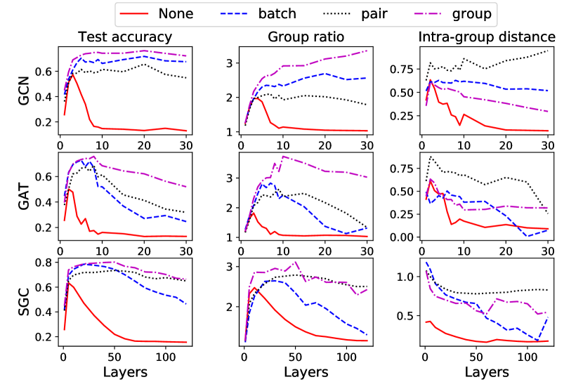
Figure 8: The test accuracy, group distance ratio and intra-group distance in Cora with missing features. We compare differentiable group normalization with none, batch and pair normalizations.

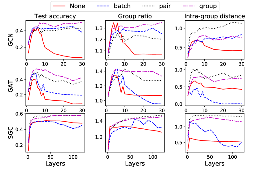
Figure 9: The test accuracy, group distance ratio and intra-group distance in Citeseer with missing features. We compare differentiable group normalization with none, batch and pair normalizations.

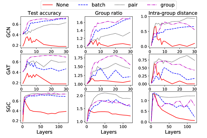
Figure 10: The test accuracy, group distance ratio and intra-group distance in Pubmed with missing features. We compare differentiable group normalization with none, batch and pair normalizations.

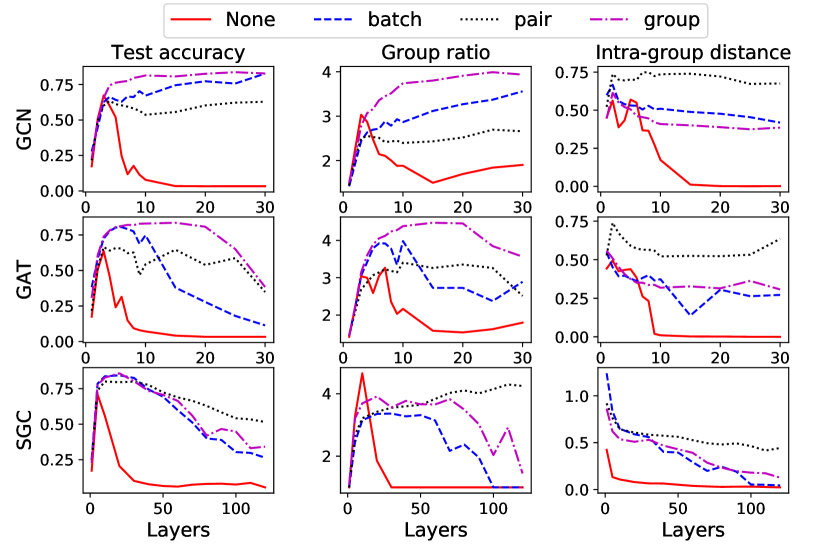
Figure 11: The test accuracy, group distance ratio and intra-group distance in CoauthorCS with missing features. We compare differentiable group normalization with none, batch and pair normalizations.

References

- [1] Franco Scarselli, Marco Gori, Ah Chung Tsoi, Markus Hagenbuchner, and Gabriele Monfardini. The graph neural network model. IEEE Transactions on Neural Networks, 20(1):61–80, 2008.
- [2] Yujia Li, Daniel Tarlow, Marc Brockschmidt, and Richard Zemel. Gated graph sequence neural networks. arXiv preprint arXiv:1511.05493, 2015.
- [3] Zonghan Wu, Shirui Pan, Fengwen Chen, Guodong Long, Chengqi Zhang, and Philip S Yu. A comprehensive survey on graph neural networks. arXiv, 2019.
- [4] David K Duvenaud, Dougal Maclaurin, Jorge Iparraguirre, Rafael Bombarell, Timothy Hirzel, Alán Aspuru-Guzik, and Ryan P Adams. Convolutional networks on graphs for learning molecular fingerprints. In NeuIPS, pages 2224–2232, 2015.
- [5] Keyulu Xu, Weihua Hu, Jure Leskovec, and Stefanie Jegelka. How powerful are graph neural networks? arXiv preprint arXiv:1810.00826, 2018.
- [6] Will Hamilton, Zhitao Ying, and Jure Leskovec. Inductive representation learning on large graphs. In NeuIPS, pages 1024–1034, 2017.
- [7] Xiao Huang, Qingquan Song, Yuening Li, and Xia Hu. Graph recurrent networks with attributed random walks. In Proceedings of the 25th ACM SIGKDD International Conference on Knowledge Discovery & Data Mining, pages 732–740, 2019.
- [8] Hongyang Gao, Zhengyang Wang, and Shuiwang Ji. Large-scale learnable graph convolutional networks. In Proceedings of the 24th ACM SIGKDD International Conference on Knowledge Discovery & Data Mining, pages 1416–1424, 2018.
- [9] Kaixiong Zhou, Qingquan Song, Xiao Huang, and Xia Hu. Auto-gnn: Neural architecture search of graph neural networks. arXiv preprint arXiv:1909.03184, 2019.
- [10] Thomas N Kipf and Max Welling. Semi-supervised classification with graph convolutional networks. ICLR, 2017.
- [11] Petar Velickovic, Guillem Cucurull, Arantxa Casanova, Adriana Romero, Pietro Lio, and Yoshua Bengio. Graph attention networks. arXiv, 1(2), 2017.
- [12] Felix Wu, Tianyi Zhang, Amauri Holanda de Souza Jr, Christopher Fifty, Tao Yu, and Kilian Q Weinberger. Simplifying graph convolutional networks. arXiv preprint arXiv:1902.07153, 2019.
- [13] Kaixiong Zhou, Qingquan Song, Xiao Huang, Daochen Zha, Na Zou, and Xia Hu. Multi-channel graph neural networks. arXiv preprint arXiv:1912.08306, 2019.
- [14] Hoang NT and Takanori Maehara. Revisiting graph neural networks: All we have is low-pass filters. arXiv preprint arXiv:1905.09550, 2019.
- [15] Miller McPherson, Lynn Smith-Lovin, and James M Cook. Birds of a feather: Homophily in social networks. Annual review of sociology, 27(1):415–444, 2001.
- [16] Qimai Li, Zhichao Han, and Xiao-Ming Wu. Deeper insights into graph convolutional networks for semi-supervised learning. In Thirty-Second AAAI Conference on Artificial Intelligence, 2018.
- [17] Kenta Oono and Taiji Suzuki. Graph neural networks exponentially lose expressive power for node classification. In International Conference on Learning Representations, 2020.
- [18] Yuening Li, Xiao Huang, Jundong Li, Mengnan Du, and Na Zou. Specae: Spectral autoencoder for anomaly detection in attributed networks. In Proceedings of the 28th ACM International Conference on Information and Knowledge Management, pages 2233–2236, 2019.
- [19] Deli Chen, Yankai Lin, Wei Li, Peng Li, Jie Zhou, and Xu Sun. Measuring and relieving the over-smoothing problem for graph neural networks from the topological view. arXiv preprint arXiv:1909.03211, 2019.
- [20] Yu Rong, Wenbing Huang, Tingyang Xu, and Junzhou Huang. Dropedge: Towards deep graph convolutional networks on node classification. In International Conference on Learning Representations. https://openreview. net/forum, 2020.
- [21] Yifan Hou, Jian Zhang, James Cheng, Kaili Ma, Richard TB Ma, Hongzhi Chen, and Ming-Chang Yang. Measuring and improving the use of graph information in graph neural networks, 2020.
- [22] Vijay Prakash Dwivedi, Chaitanya K Joshi, Thomas Laurent, Yoshua Bengio, and Xavier Bresson. Benchmarking graph neural networks. arXiv preprint arXiv:2003.00982, 2020.
- [23] Sergey Ioffe and Christian Szegedy. Batch normalization: Accelerating deep network training by reducing internal covariate shift. ICML, 2015.
- [24] Lingxiao Zhao and Leman Akoglu. Pairnorm: Tackling oversmoothing in gnns. arXiv preprint arXiv:1909.12223, 2019.
- [25] Zhilin Yang, William W Cohen, and Ruslan Salakhutdinov. Revisiting semi-supervised learning with graph embeddings. arXiv preprint arXiv:1603.08861, 2016.
- [26] Yuxin Wu and Kaiming He. Group normalization. In Proceedings of the European Conference on Computer Vision (ECCV), pages 3–19, 2018.
- [27] Alex Krizhevsky, Ilya Sutskever, and Geoffrey E Hinton. Imagenet classification with deep convolutional neural networks. In Advances in neural information processing systems, pages 1097–1105, 2012.
- [28] Justin Gilmer, Samuel S Schoenholz, Patrick F Riley, Oriol Vinyals, and George E Dahl. Neural message passing for quantum chemistry. In Proceedings of the 34th International Conference on Machine Learning-Volume 70, pages 1263–1272. JMLR. org, 2017.
- [29] Artemy Kolchinsky and Brendan D Tracey. Estimating mixture entropy with pairwise distances. Entropy, 19(7):361, 2017.
- [30] Artemy Kolchinsky, Brendan D Tracey, and David H Wolpert. Nonlinear information bottleneck. Entropy, 21(12):1181, 2019.
- [31] Guohao Li, Matthias Muller, Ali Thabet, and Bernard Ghanem. Deepgcns: Can gcns go as deep as cnns? In Proceedings of the IEEE International Conference on Computer Vision, pages 9267–9276, 2019.
- [32] Nezihe Merve Gürel, Hansheng Ren, Yujing Wang, Hui Xue, Yaming Yang, and Ce Zhang. An anatomy of graph neural networks going deep via the lens of mutual information: Exponential decay vs. full preservation. arXiv preprint arXiv:1910.04499, 2019.
- [33] Jie Zhou, Ganqu Cui, Zhengyan Zhang, Cheng Yang, Zhiyuan Liu, Lifeng Wang, Changcheng Li, and Maosong Sun. Graph neural networks: A review of methods and applications. arXiv preprint arXiv:1812.08434, 2018.
- [34] Al Mamunur Rashid, George Karypis, and John Riedl. Learning preferences of new users in recommender systems: an information theoretic approach. Acm Sigkdd Explorations Newsletter, 10(2):90–100, 2008.
- [35] Oleksandr Shchur, Maximilian Mumme, Aleksandar Bojchevski, and Stephan Günnemann. Pitfalls of graph neural network evaluation. arXiv preprint arXiv:1811.05868, 2018.
- [36] Diederik P Kingma and Jimmy Ba. Adam: A method for stochastic optimization. arXiv, 2014.
- [37] Xavier Glorot and Yoshua Bengio. Understanding the difficulty of training deep feedforward neural networks. In Proceedings of the thirteenth international conference on artificial intelligence and statistics, pages 249–256, 2010.