Multi Layer Neural Networks as Replacement for Pooling Operations

Abstract

Pooling operations, which can be calculated at low cost and serve as a linear or nonlinear transfer function for data reduction, are found in almost every modern neural network. Countless modern approaches have already tackled replacing the common maximum value selection and mean value operations, not to mention providing a function that allows different functions to be selected through changing parameters. Additional neural networks are used to estimate the parameters of these pooling functions.Consequently, pooling layers may require supplementary parameters to increase the complexity of the whole model. In this work, we show that one perceptron can already be used effectively as a pooling operation without increasing the complexity of the model. This kind of pooling allows for the integration of multi-layer neural networks directly into a model as a pooling operation by restructuring the data and, as a result, learnin complex pooling operations. We compare our approach to tensor convolution with strides as a pooling operation and show that our approach is both effective and reduces complexity. The restructuring of the data in combination with multiple perceptrons allows for our approach to be used for upscaling, which can then be utilized for transposed convolutions in semantic segmentation.

Introduction

Convolutional neural networks are the successor in many visual recognition tasks (Krizhevsky, Sutskever, and Hinton 2012; Yuan, Chen, and Wang 2019; Fuhl et al. 2019c; Fuhl, Rosenstiel, and Kasneci 2019; Fuhl et al. 2018a; Fuhl, Gao, and Kasneci 2020a; Fuhl 2020) as well as graph classification (Zhao and Wang 2019; Orsini, Frasconi, and De Raedt 2015) and time series annotation (Palaz, Collobert et al. 2015; Connor, Martin, and Atlas 1994). The main focus of modern research on CNNs includes architecture improvements (He et al. 2016; Howard et al. 2017), optimizer enhancements (Kingma and Ba 2014; Qian 1999), computational cost reduction (Rastegari et al. 2016; Fuhl et al. 2020), validation (Fuhl and Kasneci 2019), training procedures (Goodfellow et al. 2014), and also building blocks like convolutions (Long, Shelhamer, and Darrell 2015), graph kernels (Yanardag and Vishwanathan 2015) or pooling operations (Kobayashi 2019b, a; Eom and Choi 2018). The aforementioned pooling operations are used for data reduction, reducing calculation costs and making the model robust against input variations. This is especially useful in applications like eye tracking (Fuhl 2019) where the computational resources are limited and there is a plethora of information which can be extracted from the eye movements (Fuhl, Rong, and Enkelejda 2020; Fuhl et al. 2018d; Fuhl, Castner, and Kasneci 2018a, b; Fuhl and Kasneci 2018; Fuhl et al. 2019a, b). In addition, the used algorithms have to be as efficient as possible to ensure a high battery runtime (Fuhl et al. 2016b, 2017a, 2018c; Fuhl, Gao, and Kasneci 2020b; Fuhl, Santini, and Kasneci 2017b; Fuhl et al. 2018b, 2016a, 2017b; Fuhl, Santini, and Kasneci 2017a).

The pooling operation itself is inspired by the biological viewpoint of the visual cortex, based on a neuroscientific study (Hubel and Wiesel 1962). Most works suggest that max pooling is considered, biologically, to be the best operator (Riesenhuber and Poggio 1998, 1999; Serre and Poggio 2010). In practice, however, average pooling also works for CNNs, just as effectively as the combined approaches of max and average pooling. Based on this evidence, it can be surmised that the optimal pooling operation is dependent on the model, the task and the data set used. To further improve the accuracy of CNNs, simple pooling operations (e.g. max and average) are replaced by other static functions as well as by trainable operators.

The first group of operations is motivated by image scaling and uses wavelets (Mallat 1989) in wavelet pooling (Williams and Li 2018) or other image scaling techniques (Weber et al. 2016) such as detailed-preserving pooling (DPP) (Saeedan et al. 2018). Another approach is the integration of formulas that can choose between several static pooling operations like max or average pooling. The first studies in this area focus on mixed pooling and gated pooling (Lee, Gallagher, and Tu 2016; Yu et al. 2014). These selective methods have been extended with parameterizable functions that can map many different average and max pooling operations, including learned norm (Gulcehre et al. 2014) alpha (Simon et al. 2017), and alpha integration pooling (Eom and Choi 2018). The approach was further refined according to the maximum entropy principle (Kobayashi 2019b; Lee, Gallagher, and Tu 2016) and, as with alpha integration pooling (Eom and Choi 2018), equipped with parameters that can be trained and optimized in an end-to-end fashion. The global-feature guided pooling (Kobayashi 2019b) uses the input feature map to adapt pooling parameters. As a result, an additional CNN was used and jointly trained. In (Lee, Gallagher, and Tu 2016), the authors proposed mixed max average pooling, gated max average pooling, and tree pooling.

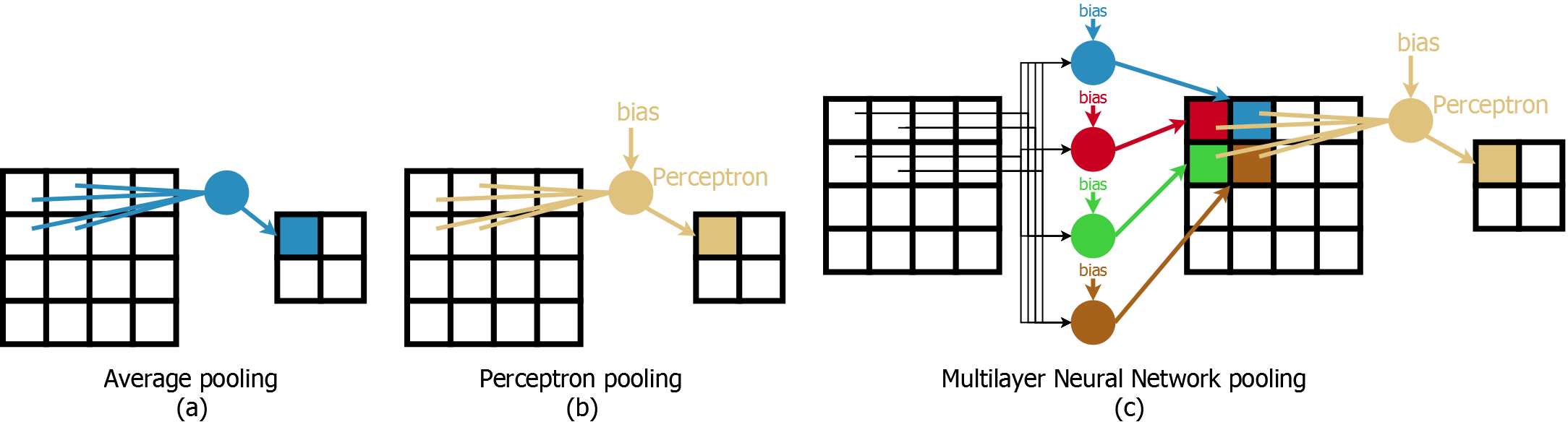
Figure 1: Visual explanation of our approach without activation functions. (a) is the average pooling operation where all weights are fixed to $0.25$. (b) is the simplest form of our approach which utilizes a perceptron as pooling operator. (c) is a multilayer neural network where the first (hidden) layer has four perceptrons and the output layer has one perceptron.

In addition to the deterministic pooling operations already mentioned, other methods that introduce randomness have been presented (Zeiler and Fergus 2013). The motivation of these pooling operations comes from drop out (Srivastava et al. 2014) and variational drop out (Kingma, Salimans, and Welling 2015). This approach can also be used in combination with all other pooling operations. Another approach which does not formulate the combination of local neuron activations as a convex mapping or downscaling operation is gaussian based pooling (Kobayashi 2019a). The authors introduce a local gaussian probabilistic model with mean and standard deviation. The deviation are estimated using global feature guided pooling (Kobayashi 2019b) and, therefore, also require an additional CNN model for parameter estimation. Alternatives to those approaches include the commonly used strided tensor convolutions (Springenberg et al. 2014). Strided tensor convolutions require multiple parameters and network in network (Lin, Chen, and Yan 2013) wherein a small multilayer perceptron is used as convolution operation. Those multilayer perceptron convolutions are stacked like normal convolution layers but do not use any data resizing. In the end, the convolutions use one global average pooling as a downscaling operation before the fully connected layers.

In contrast to other approaches, we present the simple use of perceptrons (Rosenblatt 1958) or neurons as the pooling operator. To create a deeper network from these single neurons, we propose data restructuring, allowing the data to scale up. The pooling operation that we present can be be used not only in data reduction, but also in data expansion, a key element for semantic segmentation. By the simple use of neurons or multi-layer neural networks, there is only a minimal increase in the number of parameters in need of training and the complexity of the pooling operation remains nearly the same. In comparison to the other pooling operations presented, we also compare our approach to strided tensor convolutions (Springenberg et al. 2014).

Our work contributes the latest research in the field with respect to the following points:

1

We present an efficient usage of perceptrons as pooling operation and show a

2

Perceptron-based data upscaling.

3

We provide an efficient construction of multilayer neural networks with the proposed perceptron upscaling and perceptron pooling operations and

4

Provide CUDA implementations of the proposed approach for easy integration into research and application projects.

Method

Our fundamental idea to improve learnable pooling operations is to use one of the best known function approximators available today, i.e. the neural network which consists of single neurons (also called perceptrons) and is also known as multilayer perceptron (MLP). The main advantage of an MLP is that it can be easily integrated into deep neural networks (DNNs) since it consists of the same basic components as a DNN. This makes it easy to train with the remaining layers and the same optimization methods.

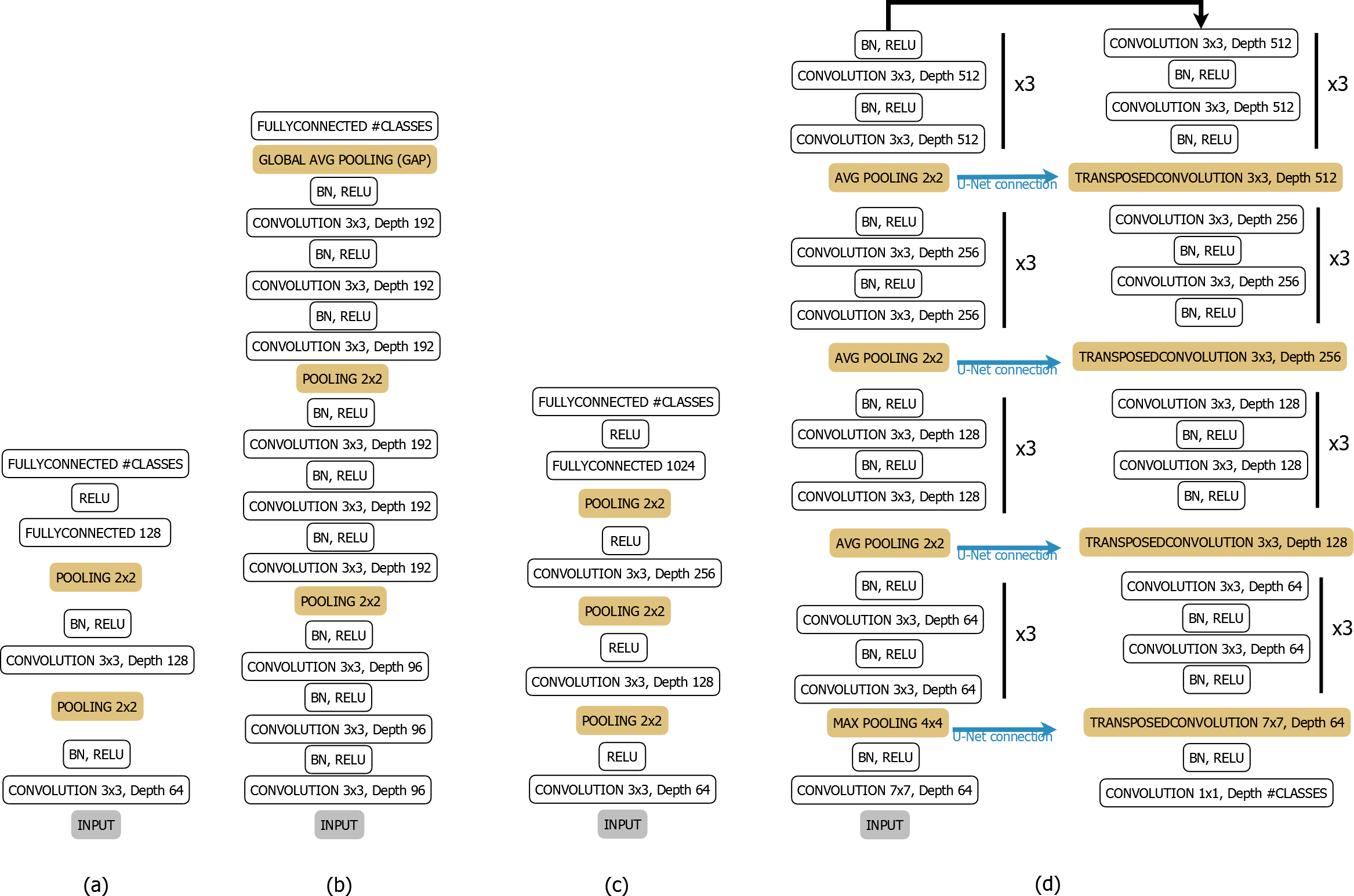
Figure 2: All used architectures in our experimental evaluation. The orange blocks are replaced with different pooling operations or in case of the transposed convolutions, the upscaling is replaced with our approach. (a) represents a small neural network model with batch normalization taken from (Eom and Choi 2018). (b) is a 14 layer architecture taken from (Kobayashi 2019a). (c) is a small model without batch normalization. (d) is a residual network using the interconnections from U-Net (Ronneberger, Fischer, and Brox 2015) for semantic image segmentation.

Figure 1 a) shows the basic concept of a pooling operation. Based on the input window, an output value is calculated, which differs depending on the selected pooling operation. Then the window is moved in the x and y dimension based on the stride parameter. If the pooling operation is average pooling, the weights (represented by the blue lines in Figure 1 a)) could be assigned the value $0.25$. Starting from here, it is easy to replace the pooling operation with a perceptron, since the only missing piece is the bias term (Figure 1 b)). The calculation of the output is nearly identical to the average pooling with the constant $0.25$ weights, which are multiplied by the corresponding input values. Afterwards, the sum is calculated together with the bias term and the activation function (ReLu (Hahnloser et al. 2000; Glorot, Bordes, and Bengio 2011), Sigmoid, TanH, etc.) of the perceptron is computed. Now we have a perceptron which is used as a pooling operation. To create a multilayer neural network, we simply use several perceptrons with activation function in the first layer and attach further perceptrons to their outputs. This idea is shown in Figure 1 c), where four perceptrons are defined for the input window of $2\times 2$ and their output is arranged in the x,y plane. For four perceptrons and a stride of two, the input tensor has the same size as the output tensor (see Figure 1 c)). One additional layer is then added on the arranged output of the four perceptrons. For the example shown in Figure 1 c), this layer consists of a perceptron with a stride of two and a window size of $2\times 2$. Thus, we have defined a neural network with a hidden layer of 4 perceptrons and an output layer of 1 perceptron, which represents our pooling operation.

The training of the perceptron or neural networks is the same as in any other layer of the superordinate neural network. As an additional memory requirement, the generated error is added, as in any other layer, to store the backpropagated error, which is needed to calculate the gradient. The only difference to the other layers in the neural network is that the learning rate of the perceptrons for the weights and the bias term should be reduced ($10^{-1}$ in our experiments). Weight decay can be used with the same reduction, but we disabled it to achieve slightly better results (Factor 0 in our experiments). It is, of course, also possible to train the perceptron or neural network for pooling at the same learning rate. In the case of large input and output tensors, however, the training becomes unstable. This is due to the fact that the error of the entire tensor affects only a few weights, and, therefore, the weights vary greatly. For example, for the nets in Figure 2 a) and c) it is possible to use the same learning rate without problems. In case of Figure 2 b) and d), however, this can lead to a initially fluctuating training phase.

A further refinement for the effective use of perceptrons or neural networks as pooling operators is the initialization of the parameters. Normally, formula 16 from (Glorot and Bengio 2010) is used for the random initialization of the parameters, which we have also used for all other layers. In the case of perceptron or neural networks, however, this can easily lead to failure. The networks only have a few parameters and, in the case of an unfavorable initialization, may not be able to shift through the gradient to a suitable minima. A simple example is the use of a perceptron for pooling with the average pooling parameter initialization. This means that each weight is set to $0.25$ and the bias term is set to $0$. Following the training of the entire model, the results of our evaluations were significantly better when compared to average pooling (see Table 1).

Table 1: Results of a single percptron with the parameter initialization from avarage pooling (each weight is set to $0.25$ and the bias term to $0$). The model a) form Figure 2 was used and evaluated on the CIFAR10 data set.

Pooling method	Run 1	Run 2	Run 3	Run 4	Run 5
Averge	84.82	84.61	84.96	85.01	84.58
(ours) Perceptron (ReLu)	84.92	84.53	84.82	85.07	84.41
(ours) Perceptron	85.94	85.76	85.92	86.16	86.06

Table 2: Results of different pooling operations for model a) from Figure 2 on the CIFAR10 data set. Our approaches are highlighted in italics. Perceptron means only a single perceptron for pooling. NN-4-1 is a multilayer neural network with 4 neurons in the first layer and 1 output neuron. NN-Z corresponds to one perceptron for pooling per layer of the input tensor. In NN-Field we used one perceptron per pooling region in the x,y plane and with NN-Tensor we used for each pooling region in the input tensor a seperate perceptron. ReLu is here the abbreviation for rectifier linear unit.

Pooling method	Accuracy on CIFAR10	Additional Parameters
Average	85.04	0
Max	84.43	0
Strided tensor convolution (ReLu) (Springenberg et al. 2014)	87.70	82,112
Strided tensor convolution (Springenberg et al. 2014)	86.78	82,112
(ours) Perceptron (ReLu)	85.22	10
(ours) Perceptron	87.71	10
(ours) Perceptron no bias (ReLu)	84.71	8
(ours) Perceptron no bias	85.11	8
(ours) NN-4-ReLu-1-ReLu	85.45	50
(ours) NN-4-ReLu-1	86.40	50
(ours) NN-4-1	87.29	50
(ours) NN-Z (ReLu)	83.87	770
(ours) NN-Z	84.37	770
(ours) NN-Field (ReLu)	84.23	1,600
(ours) NN-Field	85.28	1,600
(ours) NN-Tensor (ReLu)	81.04	122,880
(ours) NN-Tensor	80.93	122,880

Table 1 shows that the ReLu has a considerable influence on the result. We will explore this in greater detail in the first Experiment Experiment 1: Spatial Invariant vs Spatial Pooling. Consequently, for our initialization we have also used random values, but ensured that they are either symmetrical or follow rotated/mirrored patterns based on the sign of the values. This concept stems from manually created filters that originate in classical image processing, such as edge filters and weighted average pooling. In the case of a single perceptron this means: either all positive or negative and vice versa, a diagonal negative and the rest positive, or that the transition between positive and negative is along the x or y axis. For several perceptrons in the same layer, we calculated a random pattern and rotated it or mirrored it along the x or y axis, making sure that the pattern was not repeated. This was repeated until all perceptrons in the layer had an initialization.

Additional parameters for a perceptron: Each perceptron or neuron has a input window size of $W\times H$ and a bias term $b$. Therefore, we have $W*H+1$ additional parameters for a perceptron.

Additional parameters for the multilayer neural network: The amount of neurons in the first layer is $p_{1}$ and in the last layer $p_{L}$. For the first layer we would have $p_{1}*(W_{1}*H_{1}+1)$ additional parameters. Each following layer has $p_{l}*(W_{l}*H_{l}+1)$ parameters. Thus, the total number of parameters can be specified as $\sum_{l=1}^{L}p_{l}*(W_{l}*H_{l}+1)$.

Complexity of the perceptron: We perform per index value one multiplication and one addition. For the bias term we need an extra addition. Therefore, the complexity is $O(\frac{2*W*H*n}{stride^{2}}+\frac{n}{stride^{2}})$ which is theoretical $O(n)$ as for the standard pooling operations.

Complexity of the multi layer neural network: The amount of neurons in the first layer is $p_{1}$ and in the last layer $p_{L}$. Furthermore, we have $n_{l}$ input values at layer $l$. Therefore, the first layer needs $O(\frac{p_{1}*2*W_{1}*H_{1}*n_{1}}{stride_{1}^{2}}+\frac{n_{1}}{stride_{1}^{2}}))$ operations. The following layers need $O(\frac{p_{l}*2*W_{l}*H_{l}*n_{l}}{stride_{l}^{2}}+\frac{n_{l}}{stride_{l}^{2}}))$ operations. Since the amount of perceptrons or neurons per layer is independent of $n$ we still have a theoretical complexity of $O(n)$. With $stride_{l}^{2}$ we expect the same shift in each x and y dimension of the input tensor at layer $l$.

Neural Network Models

Table 3: Results of different pooling operations for model b) form Figure 2 on the CIFAR100 data set. Our approaches are highlighted in italics. Perceptron means only a single perceptron for pooling. NN-4-1 is a multilayer neural network with 4 neurons in the first layer and 1 output neuron. The same notation was used for NN-16-1 with 16 neurons in the first layer. In the last entry we also replaced the GAP layer with a perceptron.

Pooling method	Accuracy on CIFAR100	Additional Parameters
Average	75.40	0
Max	75.36	0
Strided tensor convolution (ReLu) (Springenberg et al. 2014)	77.53	184,608
Stochastic (Zeiler and Fergus 2013)	75.66	0
Mixed (Lee, Gallagher, and Tu 2016)	75.90	2
DPP (Saeedan et al. 2018)	75.56	4
Gated (Lee, Gallagher, and Tu 2016)	76.03	18
GFGP (Kobayashi 2019b)	75.81	46,080
Half-Gauss (Kobayashi 2019a)	76.74	69,840
iSP-Gauss (Kobayashi 2019a)	76.85	69,840
(ours) Perceptron	76.06	10
(ours) NN-4-1	76.21	50
(ours) NN-16-1	77.14	194
(ours) Perceptron & GAP	76.37	75

Figure 2 shows all the architectures used in our experiments. Figure 2 a) shows a small neural network we adapted from (Eom and Choi 2018) and is employed in Experiment 1 to compare different pooling operations as well as spatial pooling with fields and tensors of neurons on the CIFAR10 data set (Krizhevsky, Hinton et al. 2009). The network in Figure 2 b) was taken over from (Kobayashi 2019a) and is used for comparison with the state-oft-the-art on the CIFAR100 data set (Krizhevsky, Hinton et al. 2009) as shown in Experiment 2. The third model (Figure 2 c)) is used in Experiment 3 and does not include batch normalization. This model was employed to compare pooling operations with the same random initialization and the same batches during training. The last model in Figure 2 d) is a fully convolutional neural network (Long, Shelhamer, and Darrell 2015) with U-Net connections (Ronneberger, Fischer, and Brox 2015). It is used to compare the pooling operations and the high scaling for semantic segmentation. We implemented our approach into DLIB (King 2009) and also used it for all evaluations and comparisons.

Datasets

In this section, we present and explain training parameters for all the datasets used in our experiments. We also define the batch size as well as the optimizer and its parameters. In the case of data augmentation, we kept the number of datasets to a minimum for reproduction purposes, described in detail in the following section.

CIFAR10 (Krizhevsky, Hinton et al. 2009) consists of 60,000 $32\times 32$ colour images. The dataset has ten classes. For training, 50,000 images are provided with 5.000 examples in each class. For validation, 10,000 images are provided (1,000 examples for each class). The task in this dataset is to classify a given image to one of the ten categories.

Training: We used a batch size of 50 with a balanced amount of classes per batch and an initial learning rate of $10^{-3}$. As optimizer, we used ADAM (Kingma and Ba 2014) with weight deacay of $5*10^{-5}$, momentum one with $0.9$ and momentum two with $0.999$. For data augmentation, we cropped a $32\times 32$ region from a $40\times 40$ image, where the original image was centered on the $40\times 40$ image and the border on each side are 4 pixels set to zero. The training itself was conducted for 300 epochs, whereby the learning rate was decreased by $10^{-1}$ after each 50 epochs. The images are preprocessed by mean substraction (mean-red $122.782$, mean-green $117.001$, mean-blue $104.298$) and division by $256.0$.

CIFAR100 (Krizhevsky, Hinton et al. 2009) is similar to CIFAR10 and consists of 32x32 color images, which must be assigned to one out of 100 classes. For training, 500 examples of each class are provided. The validation set consists of 100 examples for each class. Thus, CIFAR100 has the same size as CIFAR10, with 50,000 images in the training set and 10,000 images in the validation set, respectively.

Training: We used a batch size of 100 and an initial learning rate of $10^{-1}$. As optimizer we used SGD with momentum (Qian 1999) ($0.9$) and a weight decay of ($5*10^{-4}$). For data augmentation, we normalized the images to zero mean and one standard deviation and cropped a $32\times 32$ region from a $40\times 40$ image, where the original image was centered on the $40\times 40$ image and the border on each side are 4 pixels set to zero. The training itself was conducted for 160 epochs, whereby after the 80th and 120th epoch the learning rate was decreased by $10^{-1}$. This is the same procedure as specified in (Kobayashi 2019a).

VOC2012 (Everingham et al. ) is a detection, classification and semantic segmentation dataset. We only used the semantic segmentations in our evaluation, which contains 20 classes. The task for semantic segmentation is to provide a pixelwise classification of a given image. Each image can contain multiple objects of the same class, but not all classes are present in each image. Therefore, the amount of classes increases to 21. For training, 1,464 images are provided with a total of 3,507 segmented objects. For validation, another 1,449 images are designated with a total of 3,422 segmented objects. In this dataset, the number of objects is unbalanced, making the dataset more challenging to utilize. In addition to the training and validation set’s segmented images a third set without segmentations is provided, containing 2,913 images with 6,929 objects. We did not use the third dataset in our training.

Table 4: Results of different pooling operations for model c) form Figure 2 on the CIFAR10 data set. Our approaches are highlighted in italics. Perceptron mean only a single perceptron for pooling. NN-4-1 is a multilayer neural network with 4 neurons in the first layer and 1 output neuron. Each convolution and fully connected layer had the same random initialization as well and all models saw the same batches during training.

Pooling method	Run 1	Run 2	Run 3	Run 4	Additional Parameters
Averge	84.12	84.13	84.23	84.47	0
Max	85.63	85.77	85.36	86.01	0
Strided tensor convolution (ReLu) (Springenberg et al. 2014)	86.95	87.68	87.11	87.84	344,512
(ours) Perceptron	85.73	86.13	85.95	85.18	15
(ours) NN-4-1	86.37	87.15	87.21	87.89	75

Table 5: Average pixel classification accuracy on Pascal VOC2012 sematic segmentation dataset with model d) from Figure 2. Our approaches are highlighted in italics. Perceptron is the downscaling operation (One single perceptron) and NN-4/16-UP are four/sixteen neurons for upscaling. The sixteen neurons are in the last layer before the output.

Pooling method	Pixel accuracy on VOC2012	Additional Parameters
As in Figure 2 d)	85.15	0
(ours) Perceptron & Transpose	86.36	32
(ours) Perceptron & NN-4/16-UP	87.62	172

Training: We used a batch size of 10 and an initial learning rate of $10^{-1}$. As optimizer we used SGD with momentum (Qian 1999) ($0.9$) and weight deacay ($1*10^{-4}$). For data augmentation, we used random cropping of $227\times 227$ regions with a random color offset and left right flipping of the image. The training itself was conducted for 800 epochs, whereby after each 200 epochs the learning rate was decreased by $10^{-1}$. The images are preprocessed by mean substraction (mean-red $122.782$, mean-green $117.001$, mean-blue $104.298$) and division by $256.0$.

Experiment 1: Spatial Invariant vs Spatial Pooling

Table 2 shows the comparison of different pooling operations on the CIFAR10 data set. The model chosen was a) from Figure 2. Each pooling operation was trained a total of ten times with random initialization. Of all ten runs, the best result was entered in Table 2. First, Table 2 shows that a single perceptron as a pooling operation is as good as a tensor convolution with stride. Additionally, from the Table 1 one can see that a multi-layer neural network (NN-4-1) does not perform as well. The single perceptron was also trained and evaluated without bias term and, as exhibited, it performed only slightly better than average pooling. Thus, it can be assumed that the bias term has a significant influence on this model and data set.

Another clear observation that can be obtained from this evaluation is that the ReLu (Rectifier Linear Unit) has a strong limiting influence on the classification accuracy. We believe this is the case because we used the neural network like a function embedded in a larger network. By restricting the network, we reduce the amount of functions that can be learned. Similar to a directly used neural network, the outputs are not limited. As the tiny neural networks with ReLu score significantly worse in all evaluations, we do not use the ReLu in the following experiment. For the strided tensor convolution (Springenberg et al. 2014) as pooling operation we continued with the ReLu due to better results.

As in (Lee, Gallagher, and Tu 2016) we have additionally evaluated spatially separated placements of neurons (NN-Z, NN-Field, and NN-Tensor). NN-Z is a separate perceptron for each channel of the input tensor. For the NN-Field, we assigned a single perceptron to all pooling windows in the x,y plane and moved them along the channels. In the last evaluated spatial arrangement NN-Tensor, we assigned a single perceptron to each pooling region in the input sensor. As can be seen in Table 2, the accuracy of all is significantly worse than the standard max and average pooling operations. The worst is NN-Tensor, which requires more parameters than the strided tensor convolution (Springenberg et al. 2014). Thus, we can confirm for the perceptrons that a spatial arrangement does not provide any improvement, as the authors in (Lee, Gallagher, and Tu 2016) have confirmed in their approach.

Experiment 2: Comparison to the state-of-the-art

Table 3 shows the comparison of our approach with the state-of-the-art on the CIFAR100 data set. As in (Kobayashi 2019a), we have trained each model three times with random initialization. In the end, we entered the best results in Table 2. As can be seen, the strided tensor convolution (Springenberg et al. 2014) has achieved the best results, but it also requires the most additional parameters (184,608). The second best results are obtained with the NN-16-1 neural network (97additional parameters), the iSP-Gauss (Kobayashi 2019a) (69,840 additional parameters) and the Half-Gauss (Kobayashi 2019a) (69,840 additional parameters). This is followed by the our two smaller models with a single perceptron and tiny neural network which both require significantly less additional parameters, i.e., only 50, compared to the above mentioned Gaussian-based approaches. If the global average pooling (GAP) is replaced by a perceptron, the number of parameters increases by 65 and the result improves by 0.34%. To perform training with the perceptron as a GAP replacement, we have set the learning rate factor (bias and weights) for this perceptron to $10^{-3}$. At this point, it must also be mentioned that our approach can be calculated in O(n) and we have only evaluated very small neural networks. It is, of course, also possible to use deeper and wider nets as pooling operations.

Experiment 3: Equal Randomness and Batch Data Comparison

Table 4 shows an evaluation of different pooling operations, where the same initial parameters of the convolution layers and fully connected layers are set for all. The data set used is CIFAR10 and the model is c) from Figure 2. Of course, this does not apply to the parameters of the pooling operations because of their different sizes. Also, the individual batches and the sequence of the batches were the same for all models. In this evaluation, we wanted to show a comparison between pooling operations under the same conditions. As can be seen in Table 4, the overall best result was achieved by the NN-4-1 in the fourth evaluation. Comparing the NN-4-1 with the tensor convolution, the results are always similar, whereas the tensor convolution is more stable in its range of values. A closer look at the standard pooling operations’ max and average pooling reveals that max pooling is consistently better than average pooling for this data set with the model c) from Figure 2. If we compare the individual perceptron with max and average pooling, it outperforms both in three of four runs for the model c) from Figure 2 and the CIFAR10 data set.

Experiment 4: Usage in Semantic Segmentation

Table 5 shows the result of the U-Net from Figure 2 d) on the VOC2012 data set. Each net was initialized and trained with random values. For Perceptron & Transopse we replaced only the pooling operations with a perceptron. For Perceptron & NN-4/16-UP we replaced the pooling and upscaling operations with perceptrons. As can be seen, our approach improves the results both as a pooling operation and for up scaling. Since VOC2012 is a very hard data set and semantic segmentation is a difficult task, we see this as a significant improvement of the results.

Limitations

Despite the parameter reduction presented above, our methods still have some disadvantages when compared to the classical maximum value selection or the mean value pooling. One disadvantage is that we still have a few additional parameters to calculate for the perceptron or the neural network. Additionally, this means that we have to provide memory for back-propagating the error, as is the case for each learning layer in a neural network. Of course, this also affects the optimizer, which requires needs additional memory for the moments. The use of neural networks as pooling operators also extends to the search space for model finding and, thus, their complexity and computing requirements. However, in general, our approach does not increase the complexity of the calculation of a pooling operation in the case of the perceptron, but it does improve the accuracy of the model. In the case of using a multilayer neural network for the pooling operation, our approach naturally increases the number of computations. When compared to a tensor convolution as pooling operation, however, the increase inherent in our approach is only minimal because the tensor convolution increases the complexity by the output tensor depth. As a general remark, it must also be said that, in case of unstable training, reducing the learning rate of the perceptron or small neural network has always resulted in success.

Conclusion

In this paper, we have shown that single perceptrons can be used effectively as pooling operators without increasing the complexity of the model. We have also shown that neural networks can be formed as pooling operators by simply restructuring the output data of several perceptrons. This increases the complexity and number of parameters in the model only minimally compared to tensor convolutions as pooling operator and is almost as effective. These multi-layer neural networks and presented restructuring can also be used to learn a scaling that can be effectively employed for transposed convolutions. Here it is also possible to learn the scaling via tensors. This would require an extension of our approach utilizing two dimensional matrices. In addition to the models evaluated in this paper, it is, of course, possible to train deeper nets as pooling operators or to equip individual layers with more perceptrons. In this way, the results can be further improved. We leave this open for future research. Our approach is easy to integrate into modern architectures and can be learned simultaneously with all other parameters without creating parallel branches in a model. Thus, the approach can also be effectively computed on a GPU.

References

- Connor, Martin, and Atlas (1994) Connor, J. T.; Martin, R. D.; and Atlas, L. E. 1994. Recurrent neural networks and robust time series prediction. IEEE transactions on neural networks 5(2): 240–254.
- Eom and Choi (2018) Eom, H.; and Choi, H. 2018. Alpha-Integration Pooling for Convolutional Neural Networks. arXiv preprint arXiv:1811.03436 .
- (3) Everingham, M.; Van Gool, L.; Williams, C. K. I.; Winn, J.; and Zisserman, A. ???? The PASCAL Visual Object Classes Challenge 2012 (VOC2012) Results. http://www.pascal-network.org/challenges/VOC/voc2012/workshop/index.html.
- Fuhl (2019) Fuhl, W. 2019. Image-based extraction of eye features for robust eye tracking. Ph.D. thesis, University of Tübingen.
- Fuhl (2020) Fuhl, W. 2020. From perception to action using observed actions to learn gestures. User Modeling and User-Adapted Interaction 1–18.
- Fuhl et al. (2019a) Fuhl, W.; Bozkir, E.; Hosp, B.; Castner, N.; Geisler, D.; Santini, T. C.; and Kasneci, E. 2019a. Encodji: encoding gaze data into emoji space for an amusing scanpath classification approach. In Proceedings of the 11th ACM Symposium on Eye Tracking Research & Applications, 1–4.
- Fuhl, Castner, and Kasneci (2018a) Fuhl, W.; Castner, N.; and Kasneci, E. 2018a. Histogram of oriented velocities for eye movement detection. In International Conference on Multimodal Interaction Workshops, ICMIW.
- Fuhl, Castner, and Kasneci (2018b) Fuhl, W.; Castner, N.; and Kasneci, E. 2018b. Rule based learning for eye movement type detection. In International Conference on Multimodal Interaction Workshops, ICMIW.
- Fuhl et al. (2019b) Fuhl, W.; Castner, N.; Kübler, T. C.; Lotz, A.; Rosenstiel, W.; and Kasneci, E. 2019b. Ferns for area of interest free scanpath classification. In Proceedings of the 2019 ACM Symposium on Eye Tracking Research & Applications (ETRA).
- Fuhl et al. (2018a) Fuhl, W.; Castner, N.; Zhuang, L.; Holzer, M.; Rosenstiel, W.; and Kasneci, E. 2018a. MAM: Transfer learning for fully automatic video annotation and specialized detector creation. In International Conference on Computer Vision Workshops, ICCVW.
- Fuhl et al. (2018b) Fuhl, W.; Eivazi, S.; Hosp, B.; Eivazi, A.; Rosenstiel, W.; and Kasneci, E. 2018b. BORE: Boosted-oriented edge optimization for robust, real time remote pupil center detection. In Eye Tracking Research and Applications, ETRA.
- Fuhl, Gao, and Kasneci (2020a) Fuhl, W.; Gao, H.; and Kasneci, E. 2020a. Neural networks for optical vector and eye ball parameter estimation. In ACM Symposium on Eye Tracking Research & Applications, ETRA 2020. ACM.
- Fuhl, Gao, and Kasneci (2020b) Fuhl, W.; Gao, H.; and Kasneci, E. 2020b. Tiny convolution, decision tree, and binary neuronal networks for robust and real time pupil outline estimation. In ACM Symposium on Eye Tracking Research & Applications, ETRA 2020. ACM.
- Fuhl et al. (2019c) Fuhl, W.; Geisler, D.; Rosenstiel, W.; and Kasneci, E. 2019c. The applicability of Cycle GANs for pupil and eyelid segmentation, data generation and image refinement. In International Conference on Computer Vision Workshops, ICCVW.
- Fuhl et al. (2018c) Fuhl, W.; Geisler, D.; Santini, T.; Appel, T.; Rosenstiel, W.; and Kasneci, E. 2018c. CBF:Circular binary features for robust and real-time pupil center detection. In ACM Symposium on Eye Tracking Research & Applications.
- Fuhl and Kasneci (2018) Fuhl, W.; and Kasneci, E. 2018. Eye movement velocity and gaze data generator for evaluation, robustness testing and assess of eye tracking software and visualization tools. In Poster at Egocentric Perception, Interaction and Computing, EPIC.
- Fuhl and Kasneci (2019) Fuhl, W.; and Kasneci, E. 2019. Learning to validate the quality of detected landmarks. In International Conference on Machine Vision, ICMV.
- Fuhl et al. (2020) Fuhl, W.; Kasneci, G.; Rosenstiel, W.; and Kasneci, E. 2020. Training Decision Trees as Replacement for Convolution Layers. In Conference on Artificial Intelligence, AAAI.
- Fuhl et al. (2017a) Fuhl, W.; Kübler, T. C.; Hospach, D.; Bringmann, O.; Rosenstiel, W.; and Kasneci, E. 2017a. Ways of improving the precision of eye tracking data: Controlling the influence of dirt and dust on pupil detection. Journal of Eye Movement Research 10(3).
- Fuhl, Rong, and Enkelejda (2020) Fuhl, W.; Rong, Y.; and Enkelejda, K. 2020. Fully Convolutional Neural Networks for Raw Eye Tracking Data Segmentation, Generation, and Reconstruction. In Proceedings of the International Conference on Pattern Recognition, 0–0.
- Fuhl, Rosenstiel, and Kasneci (2019) Fuhl, W.; Rosenstiel, W.; and Kasneci, E. 2019. 500,000 images closer to eyelid and pupil segmentation. In Computer Analysis of Images and Patterns, CAIP.
- Fuhl et al. (2017b) Fuhl, W.; Santini, T.; Geisler, D.; Kübler, T. C.; and Kasneci, E. 2017b. EyeLad: Remote Eye Tracking Image Labeling Tool. In 12th Joint Conference on Computer Vision, Imaging and Computer Graphics Theory and Applications (VISIGRAPP 2017).
- Fuhl et al. (2016a) Fuhl, W.; Santini, T.; Geisler, D.; Kübler, T. C.; Rosenstiel, W.; and Kasneci, E. 2016a. Eyes Wide Open? Eyelid Location and Eye Aperture Estimation for Pervasive Eye Tracking in Real-World Scenarios. In ACM International Joint Conference on Pervasive and Ubiquitous Computing: Adjunct publication – PETMEI 2016.
- Fuhl, Santini, and Kasneci (2017a) Fuhl, W.; Santini, T.; and Kasneci, E. 2017a. Fast and Robust Eyelid Outline and Aperture Detection in Real-World Scenarios. In IEEE Winter Conference on Applications of Computer Vision (WACV 2017).
- Fuhl, Santini, and Kasneci (2017b) Fuhl, W.; Santini, T.; and Kasneci, E. 2017b. Fast camera focus estimation for gaze-based focus control. In CoRR.
- Fuhl et al. (2018d) Fuhl, W.; Santini, T.; Kuebler, T.; Castner, N.; Rosenstiel, W.; and Kasneci, E. 2018d. Eye movement simulation and detector creation to reduce laborious parameter adjustments. arXiv preprint arXiv:1804.00970 .
- Fuhl et al. (2016b) Fuhl, W.; Santini, T.; Reichert, C.; Claus, D.; Herkommer, A.; Bahmani, H.; Rifai, K.; Wahl, S.; and Kasneci, E. 2016b. Non-Intrusive Practitioner Pupil Detection for Unmodified Microscope Oculars. Elsevier Computers in Biology and Medicine 79: 36–44.
- Glorot and Bengio (2010) Glorot, X.; and Bengio, Y. 2010. Understanding the difficulty of training deep feedforward neural networks. In Proceedings of the thirteenth international conference on artificial intelligence and statistics, 249–256.
- Glorot, Bordes, and Bengio (2011) Glorot, X.; Bordes, A.; and Bengio, Y. 2011. Deep sparse rectifier neural networks. In Proceedings of the fourteenth international conference on artificial intelligence and statistics, 315–323.
- Goodfellow et al. (2014) Goodfellow, I.; Pouget-Abadie, J.; Mirza, M.; Xu, B.; Warde-Farley, D.; Ozair, S.; Courville, A.; and Bengio, Y. 2014. Generative adversarial nets. In Advances in neural information processing systems, 2672–2680.
- Gulcehre et al. (2014) Gulcehre, C.; Cho, K.; Pascanu, R.; and Bengio, Y. 2014. Learned-norm pooling for deep feedforward and recurrent neural networks. In Joint European Conference on Machine Learning and Knowledge Discovery in Databases, 530–546. Springer.
- Hahnloser et al. (2000) Hahnloser, R. H.; Sarpeshkar, R.; Mahowald, M. A.; Douglas, R. J.; and Seung, H. S. 2000. Digital selection and analogue amplification coexist in a cortex-inspired silicon circuit. Nature 405(6789): 947–951.
- He et al. (2016) He, K.; Zhang, X.; Ren, S.; and Sun, J. 2016. Deep residual learning for image recognition. In Proceedings of the IEEE conference on computer vision and pattern recognition, 770–778.
- Howard et al. (2017) Howard, A. G.; Zhu, M.; Chen, B.; Kalenichenko, D.; Wang, W.; Weyand, T.; Andreetto, M.; and Adam, H. 2017. Mobilenets: Efficient convolutional neural networks for mobile vision applications. arXiv preprint arXiv:1704.04861 .
- Hubel and Wiesel (1962) Hubel, D. H.; and Wiesel, T. N. 1962. Receptive fields, binocular interaction and functional architecture in the cat’s visual cortex. The Journal of physiology 160(1): 106–154.
- King (2009) King, D. E. 2009. Dlib-ml: A machine learning toolkit. Journal of Machine Learning Research 10(Jul): 1755–1758.
- Kingma and Ba (2014) Kingma, D. P.; and Ba, J. 2014. Adam: A method for stochastic optimization. arXiv preprint arXiv:1412.6980 .
- Kingma, Salimans, and Welling (2015) Kingma, D. P.; Salimans, T.; and Welling, M. 2015. Variational dropout and the local reparameterization trick. In Advances in neural information processing systems, 2575–2583.
- Kobayashi (2019a) Kobayashi, T. 2019a. Gaussian-Based Pooling for Convolutional Neural Networks. In Advances in Neural Information Processing Systems, 11214–11224.
- Kobayashi (2019b) Kobayashi, T. 2019b. Global Feature Guided Local Pooling. In Proceedings of the IEEE International Conference on Computer Vision, 3365–3374.
- Krizhevsky, Hinton et al. (2009) Krizhevsky, A.; Hinton, G.; et al. 2009. Learning multiple layers of features from tiny images .
- Krizhevsky, Sutskever, and Hinton (2012) Krizhevsky, A.; Sutskever, I.; and Hinton, G. E. 2012. Imagenet classification with deep convolutional neural networks. In Advances in neural information processing systems, 1097–1105.
- Lee, Gallagher, and Tu (2016) Lee, C.-Y.; Gallagher, P. W.; and Tu, Z. 2016. Generalizing pooling functions in convolutional neural networks: Mixed, gated, and tree. In Artificial intelligence and statistics, 464–472.
- Lin, Chen, and Yan (2013) Lin, M.; Chen, Q.; and Yan, S. 2013. Network in network. arXiv preprint arXiv:1312.4400 .
- Long, Shelhamer, and Darrell (2015) Long, J.; Shelhamer, E.; and Darrell, T. 2015. Fully convolutional networks for semantic segmentation. In Proceedings of the IEEE conference on computer vision and pattern recognition, 3431–3440.
- Mallat (1989) Mallat, S. G. 1989. A theory for multiresolution signal decomposition: the wavelet representation. IEEE transactions on pattern analysis and machine intelligence 11(7): 674–693.
- Orsini, Frasconi, and De Raedt (2015) Orsini, F.; Frasconi, P.; and De Raedt, L. 2015. Graph invariant kernels. In Twenty-Fourth International Joint Conference on Artificial Intelligence.
- Palaz, Collobert et al. (2015) Palaz, D.; Collobert, R.; et al. 2015. Analysis of cnn-based speech recognition system using raw speech as input. Technical report, Idiap.
- Qian (1999) Qian, N. 1999. On the momentum term in gradient descent learning algorithms. Neural networks 12(1): 145–151.
- Rastegari et al. (2016) Rastegari, M.; Ordonez, V.; Redmon, J.; and Farhadi, A. 2016. Xnor-net: Imagenet classification using binary convolutional neural networks. In European conference on computer vision, 525–542. Springer.
- Riesenhuber and Poggio (1998) Riesenhuber, M.; and Poggio, T. 1998. Just one view: Invariances in inferotemporal cell tuning. In Advances in neural information processing systems, 215–221.
- Riesenhuber and Poggio (1999) Riesenhuber, M.; and Poggio, T. 1999. Hierarchical models of object recognition in cortex. Nature neuroscience 2(11): 1019–1025.
- Ronneberger, Fischer, and Brox (2015) Ronneberger, O.; Fischer, P.; and Brox, T. 2015. U-net: Convolutional networks for biomedical image segmentation. In International Conference on Medical image computing and computer-assisted intervention, 234–241. Springer.
- Rosenblatt (1958) Rosenblatt, F. 1958. The perceptron: a probabilistic model for information storage and organization in the brain. Psychological review 65(6): 386.
- Saeedan et al. (2018) Saeedan, F.; Weber, N.; Goesele, M.; and Roth, S. 2018. Detail-preserving pooling in deep networks. In Proceedings of the IEEE Conference on Computer Vision and Pattern Recognition, 9108–9116.
- Serre and Poggio (2010) Serre, T.; and Poggio, T. 2010. A neuromorphic approach to computer vision. Communications of the ACM 53(10): 54–61.
- Simon et al. (2017) Simon, M.; Gao, Y.; Darrell, T.; Denzler, J.; and Rodner, E. 2017. Generalized orderless pooling performs implicit salient matching. In Proceedings of the IEEE international conference on computer vision, 4960–4969.
- Springenberg et al. (2014) Springenberg, J. T.; Dosovitskiy, A.; Brox, T.; and Riedmiller, M. 2014. Striving for simplicity: The all convolutional net. arXiv preprint arXiv:1412.6806 .
- Srivastava et al. (2014) Srivastava, N.; Hinton, G.; Krizhevsky, A.; Sutskever, I.; and Salakhutdinov, R. 2014. Dropout: a simple way to prevent neural networks from overfitting. The journal of machine learning research 15(1): 1929–1958.
- Weber et al. (2016) Weber, N.; Waechter, M.; Amend, S. C.; Guthe, S.; and Goesele, M. 2016. Rapid, detail-preserving image downscaling. ACM Transactions on Graphics (TOG) 35(6): 1–6.
- Williams and Li (2018) Williams, T.; and Li, R. 2018. Wavelet pooling for convolutional neural networks .
- Yanardag and Vishwanathan (2015) Yanardag, P.; and Vishwanathan, S. 2015. Deep graph kernels. In Proceedings of the 21th ACM SIGKDD International Conference on Knowledge Discovery and Data Mining, 1365–1374.
- Yu et al. (2014) Yu, D.; Wang, H.; Chen, P.; and Wei, Z. 2014. Mixed pooling for convolutional neural networks. In International conference on rough sets and knowledge technology, 364–375. Springer.
- Yuan, Chen, and Wang (2019) Yuan, Y.; Chen, X.; and Wang, J. 2019. Object-Contextual Representations for Semantic Segmentation. arXiv preprint arXiv:1909.11065 .
- Zeiler and Fergus (2013) Zeiler, M. D.; and Fergus, R. 2013. Stochastic pooling for regularization of deep convolutional neural networks. arXiv preprint arXiv:1301.3557 .
- Zhao and Wang (2019) Zhao, Q.; and Wang, Y. 2019. Learning metrics for persistence-based summaries and applications for graph classification. In Advances in Neural Information Processing Systems, 9855–9866.