Early Detection of Retinopathy of Prematurity (ROP) in Retinal Fundus Images Via Convolutional Neural Networks

Abstract

Retinopathy of prematurity (ROP) is an abnormal blood vessel development in the retina of a prematurely-born infant or an infant with low birth weight. ROP is one of the leading causes for infant blindness globally. Early detection of ROP is critical to slow down and avert the progression to vision impairment caused by ROP. Yet there is limited awareness of ROP even among medical professionals. Consequently, dataset for ROP is limited if ever available, and is in general extremely imbalanced in terms of the ratio between negative images and positive ones.

In this study, we formulate the problem of detecting ROP in retinal fundus images in an optimization framework, and apply state-of-art convolutional neural network techniques to solve this problem. Experimental results based on our models achieve 100 percent sensitivity, 96 percent specificity, 98 percent accuracy, and 96 percent precision. In addition, our study shows that as the network gets deeper, more significant features can be extracted for better understanding of ROP.

1 Introduction

Retinopathy of prematurity (ROP) is an abnormal blood vessel development in the retina of prematurely-born infants or infants with low birth weight [3]. ROP can lead to permanent visual impairment and is one of the leading causes of infant blindness globally. Higher neonatal survival rates have significantly increased the number of premature infants; consequently, there are sharp increases in ROP cases for infants. It is estimated that nineteen million children are visually impaired worldwide [1], among which ROP accounts for six to eighteen percent in childhood blindness [4]. Early treatment has confirmed the efficacy of treatment for ROP [2]. Therefore, it is crucial that at-risk infants receive timely retinal examinations and early detection of potential ROP.

Early detection of ROP faces significant challenges. The most imposing one is the dire lack of experienced ophthalmologists for the screen of ROP, even in developed countries. This challenge is compounded by the limited awareness of ROP even among medical professionals and infants’ inability of active participation in medical diagnosis.

Deep learning has made significant progresses in image classification and pattern recognition, and has shown great potentials for applications in medical images, such as of diabetic retinopathy (DR) [5]. However, the development of high-performance deep learning methodology for medical imaging has two critical requirements. First, it requires collections of large datasets with tens of thousands of abnormal (positive) cases. Secondly, clinical validation datasets for evaluation of final performance require multiple grades for each image to ensure the consistency of the grading result. For instance, DR is a well-recognized complication among tens of millions of diabetic patients and the available datasets with both positive and negative samples from DR diagnosis are in the order of several hundred thousands. In the case of ROP, however, it is infeasible to meet these two key requirements. Due to the limited awareness and expertise among medical professionals, ROP dataset is limited and extremely imbalanced in terms of the ratio between negative and positive images. (See Section 2). More importantly, clinical screening for ROP often requires unusually high sensitivity level, i.e., higher than the medical standard of 95%. This is to ensure that few positive ROP cases are missed for infants.

Our work.

We formulate the problem of identifying ROP from retinal fundus images in an optimization framework, and adopt neural network techniques to solve this optimization problem.

Our study consists of two stages. First, we use a shallow convolutional neural network called ROPBaseCNN. This ROPBaseCNN-based model works well and achieves over 91 percent in both specificity and sensitivity on the first dataset Data_0 collected from a single data source. To increase the robustness of the model, more ROP data Data_1 from multiple data sources are collected, and a deeper neural network ROPResCNN is developed. This updated ROPResCNN-based model overcomes the over-fitting and vanishing/exploding gradient problem.

Our experiments demonstrate that ROPResCNN-based model dominates both human experts and ROPBaseCNN-model, by a wide margin. It shows impressive performance on the combined Data_0 and Data_1: a perfect score on sensitivity, excellent scores of specificity (96%) and precision (96%), and across-the-board improvement of roughly 10% when compared with experienced ophthalmologists. Most importantly, it reduces human errors by over 66% in all categories, and in particular eliminates completely the error in the category of sensitivity, the most critical requirement for diagnosis of ROP.

In addition to excellent experimental results, our study shows that as the network gets deeper, significant features can be extracted for better understanding of ROP. For instance, in spite of the limited and imbalanced data, ROPResCNN-based model succeeds in learning and capturing explicitly a well-known indicator for the medical diagnosis of ROP.

2 ROP: Data Collection, Augmentation, and Processing

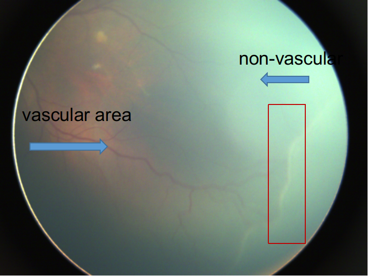
(a) Positive sample

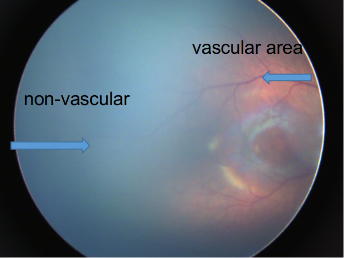
(b) Negative sample

Figure 1: positive sample and negative sample in Data_0; the difference between the vascular area and the non-vascular area is clear; note the apparent thickened ridge (indicated in the red box) in the positive sample between the vascular and the non-vascular areas, with no such appearance in the negative sample.

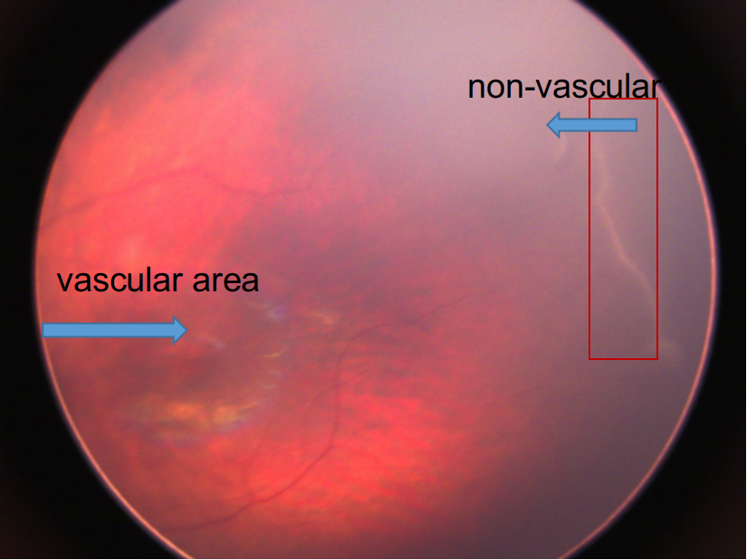
(a) Positive sample

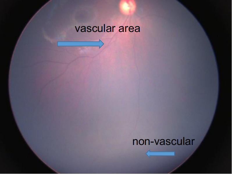
(b) Negative sample

Figure 2: positive sample and negative sample in Data_1; note the thickened white line (indicated in the red box) in the positive sample between the vascular and the non-vascular areas.

2.1 Data Collection

To develop a model for ROP detection, ROP retinal fundus images were retrospectively collected from the Affiliated Eye Hospital of Nanchang University, which is an AAA (i.e., the highest ranked) hospital in China. All images were de-identified according to patient privacy protection policy, and ethics review was approved by the ethical committee of the university.

Two datasets were used. The first de-identified dataset, Data_0, consists of random samples of ROP images taken at the hospital between 2013 and 2018. A single type of fundus camera, Clarity Retcam3, was used with 130°fields of view. All operators had gone through professional training. Data_0 includes 2021 negative samples and 382 positive samples with the resolution of $1600\times 1200$ retinal fundus image. Images in this dataset share a common characteristic: the boundary between the vascular and the non-vascular areas is clear and the color difference is obvious. As shown in Figure 1, there is a clear white dividing line, called the demarcation line, between the vascular and the non-vascular areas of the peripheral retina. In the early stage of ROP, this demarcation line will get thicker until a ridge occurs. As the ridge gets thicker, proliferation of abnormal blood vessels will cause the retinal blood vessel to expand, eventually leading to the ROP problem. The appearance of thickened ridges is the main indicator used by ophthalmologists to diagnose ROP. Note that there is no such thickened ridge in the negative sample.

The second de-identified dataset Data_1 consists of 461 negative samples and 498 positive samples with the resolution of $1600\times 1200$ retinal fundus images. A variety of 130°fields cameras were used, including CLARITY Retcam3, SUOER SW-8000, and MEDSO ORTHOCONE RS-B002. This set of data is characterized by the similar appearance of the vascular and non-vascular areas, and with similar colors. However, the boundary between the vascular area and the non-vascular area is much clearer than that in Data_0. Figure 2 shows a negative sample and a positive sample from Data_1.

All images were graded by ophthalmologists for the presence of ROP severity and for the image quality using an annotation tool. The annotation tool was designed by ophthalmologists and implemented by ourselves. ROP severity was graded as positive or negative. Image quality was assessed by graders, with images of adequate quality considered gradable. The reliability of the grading result was assessed by four prominent ophthalmologists. The final grading results, for which the diagnosis from the hospital agreed with the majority of diagnosis from these ophthalmologists, were used for each retinal fundus image.

2.2 Data Processing and Balancing

The datasets are imbalanced, for instance, negative samples in Data_0 dataset is five times more than positive samples. Consequently, the training process may be significantly biased towards the class with more samples. Data imbalance is very common among medical data. There are several approaches, including under-sampling [6], re-sampling and fine-tuning [7], oversampling [11], and weight balance and class balance [13].

To mitigate the imbalance problem, we design a hybrid method with a combination of several techniques:

1. Data enhancement: all samples in the dataset are first enhanced by brightness adjustment and random flipping. (See Figure 3). Afterwards, all images are resized into $300\times 300$.

2. Tuning sampling ratio and class weights: we use different class weights in the cross entropy loss function in our optimization framework, to be introduced in the next section. We over-sample the enhanced positive samples and re-sample the enhanced negative samples, so that the numbers of positive samples and negative samples in the sample batch are kept proportional to the inverse of their class weights. We experiment with different ratios through grid search in the validation set, and eventually set the ratio of positive and negative samples to $1:2$ in the training process.

This data processing and balance strategy is used throughout our study.

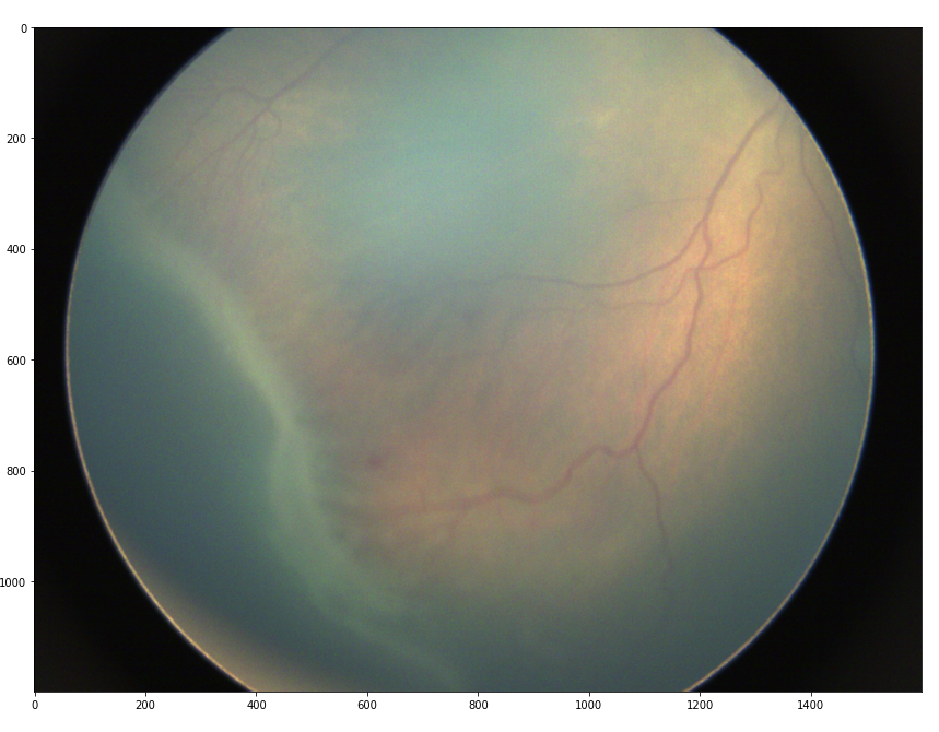
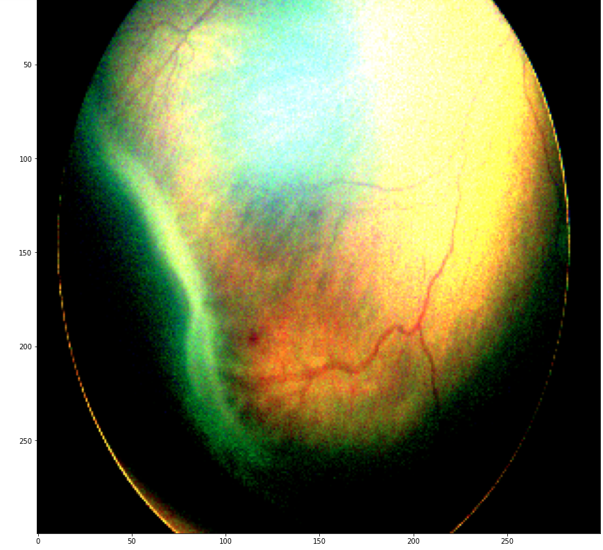
Figure 3: the left is an original retinal fundus image; the right is the same image from the left after data processing.

3 Problem and Optimization

Problem formulation.

We formulate the problem of detecting ROP as a binary classification problem, where the positive images and the negative images are labeled as $1$ and $0$, respectively. That is, given a fundus image, instead of labelling the image as either $1$ or $0$, we assign a score in terms of probability between $0$ and $1$ to the input image. The higher the score, the higher the probability that the image has an ROP (i.e., ROP positive). When assigning the label for the input image, if the probability is higher than $0.5$, it is then labelled as positive; otherwise it is negative. This is a natural choice for the neural network which requires the output to be a continuous variable.

Now, suppose the probability is parametrized by $\theta$ such that it is denoted as $p_{\theta}$. This set of parameter could be interpreted as various factors contributing to the probability of having an ROP. Then the training stage is to minimize the cross entropy loss function over the set of parameters $\theta$. That is, denote the distribution of the pair of the image $x$ and the 0-1 label $y$ by $p_{\text{data}}$, then the training process is to solve the following optimization problem,

$$\min_{\theta}\mathbb{E}_{(x,y)\sim p_{\text{data}}}[-y\log p_{\theta}(x)-(1-y)\log(1-p_{\theta}(x))].$$

Given the limited amount of available data and hence possible issue of overfitting, we add a kernel regularization. In particular, we adopt the $L^{2}$ regularization on the weight matrices of the fully connected layers. For each fully connected layer with weight matrix $W=(w_{ij})$, we add the following regularization term to the loss function

$$\lambda\|W\|_{L^{2}}=\lambda\sum_{i,j}w_{ij}^{2},$$

where $\lambda$ is a hyperparameter to adjust the scale of the regularization. Finally, we adjust the loss function by the $1:2$ class weight from the data processing stage, so that the final optimization problem is to solve the following regularized cross entropy loss function,

$$\min_{\theta}\mathbb{E}_{(x,y)\sim p_{\text{data}}}[-y\log p_{\theta}(x)-2(1-y)\log(1-p_{\theta}(x))]+\lambda\|W\|_{L^{2}}.$$ (1)

Optimization.

We used the Adam algorithm [9] to solve our optimization problem (1). Adam algorithm combines a momentum method and an adaptive learning rate method, and uses the first order and the second order moments to optimize the neural network which is to be specified in details in section 4. Adam algorithm is more efficient than the vanilla stochastic gradient descent algorithm.

The parameters of Adam algorithm used here are: learning rate $\alpha=0.001$, and the exponential decay rate for the first and the second moment $\beta_{1}=0.9$ and $\beta_{2}=0.999$, respectively.

To train our models more efficiently, we adjust the learning rate with respect to the validation loss. More specifically, the learning rate is reduced by 20% when the validation loss does not improve for $5$ epochs.

Algorithm 1 Adam is proposed for stochastic optimization. Default settings are $\alpha$ = 0.001, $\beta_{1}$ = 0.9, $\beta_{2}$ = 0.999, $\eta=10^{-7}$, $r=0.8$, and $n=5$.

$\alpha$: Learning rate

$\beta_{1},\beta_{2}$: $\in$ [0, 1): Exponential decay rates for the moment estimates

$f(\theta)$: Stochastic objective function with parameters $\theta$

$\theta$: Initial parameter vector

$r$: Learning rate reduction factor

$n$: Patience parameter

$m_{0}$ $\leftarrow$ 0: Initialize $1^{st}$ moment vector

$v_{0}$ $\leftarrow$ 0: Initialize $2^{nd}$ moment vector

$i$ $\leftarrow$ 0: Initialize step

while $\theta_{i}$ not converged do

     $i\leftarrow i+1$

     $g_{i}$ $\leftarrow$ $\nabla_{\theta}$$f_{i}(\theta_{i-1})$ (Get gradients stochastic objective at step i)

     $m_{i}$ $\leftarrow$ $\beta_{1}$ $\cdot$ $m_{i-1}$+($1-\beta_{1}$)$\cdot g_{i}$ (Update biased first moment estimate)

     $v_{i}$ $\leftarrow$ $\beta_{2}$ $\cdot$ $v_{i-1}$+($1-\beta_{2}$)$\cdot g_{i}^{2}$ ((Update biased second raw moment estimate)

     $\hat{m}_{i}$ $\leftarrow$ $m_{i}/(1-\beta_{1}^{i}$)(Compute bias-corrected first moment estimate)

     $\hat{v}_{i}$ $\leftarrow$ $v_{i}/(1-\beta_{2}^{i}$)(Compute bias-corrected second raw moment estimate)

     $\theta_{i}$ $\leftarrow$ $\theta_{i-1}-\alpha\cdot$ $\hat{m}_{i}/(\sqrt[2]{\hat{v}_{i}}+\eta)$ (Update parameters)

     $\alpha\leftarrow r\alpha$ if the validation result does not improve for $n$ steps.

end while

return $\theta_{i}$ (Resulting parameter)

4 Convolutional Neural Network and Architectures

The network adopted here is the convolutional neural network (CNN) [10]. CNN is specialized for processing grid-like data including images. A CNN consists of the feature extractor and the decoder. The feature extractor has several convolutional layers and pooling layers. It captures the basic features such as lines and corners in the first few layers and extracts more advanced features such as the indicators of ROP in the later layers. The extracted features are then fed into the decoder part. The decoder is a set of fully connected layers. The decoder uses the extracted features to predict the target variable. In our problem, the probability of an input image having ROP is the target variable. We experiment with two different architectures for CNN: ROPBaseCNN and ROPResCNN.

Type of layer	parameters
Input	shape=(300,300,3)
Convolution	filters=32, kernel size=$3\times 3$, stride2=(2,2), activation=ReLU
Max pooling	pool size=$2\times 2$, strides=(2,2)
Convolution	filters=64, kernel size=$3\times 3$, stride2=(2,2), activation=ReLU
Max pooling	pool size=$2\times 2$, strides=(2,2)
Dropout	dropping probability = 0.25
Flatten	none
Fully connected	neurons=128, activation=ReLU, $\lambda=0.001$
Dropout	dropping probability = 0.5
Fully connected	neurons=64, activation=ReLU, $\lambda=0.001$
Output(Dense)	shape=(1), activation=sigmoid

Figure 4: the architecture of ROPBaseCNN

model	ROPBaseCNN	ROPBaseCNN	ROPResCNN
Train data	Data_0	Data_0+Data_1	Data_0+Data_1
Test data	Data_0	Data_0+Data_1	Data_0+Data_1
Precision	0.9479	0.8131	0.96
Sensitivity	0.91	0.7891	1.0
Specificity	0.9135	0.9335	0.96
Accuracy	0.93	0.8948	0.98
F1 score	0.9286	0.8009	0.98

Figure 5: experimental results with data Data_0 and Data_1

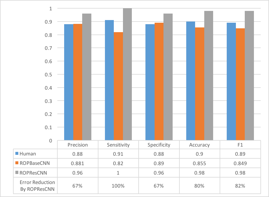
Figure 6: comparison between ophthalmologists and our models

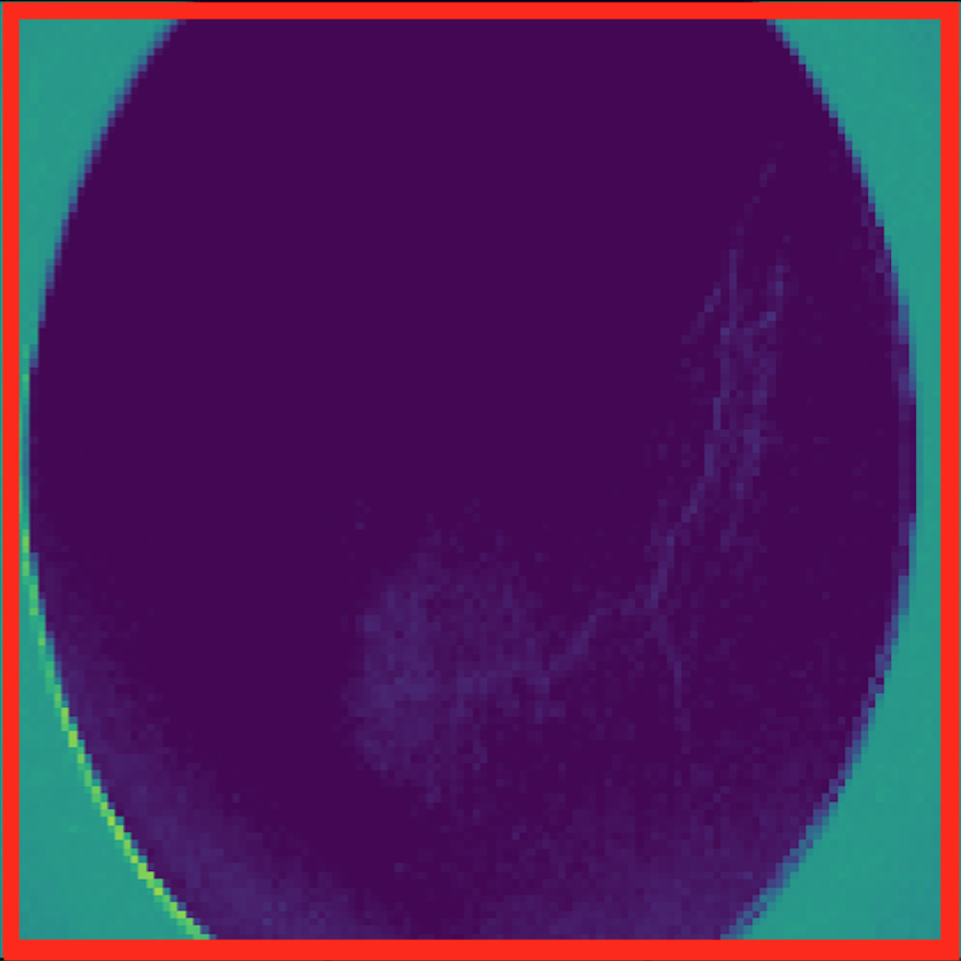
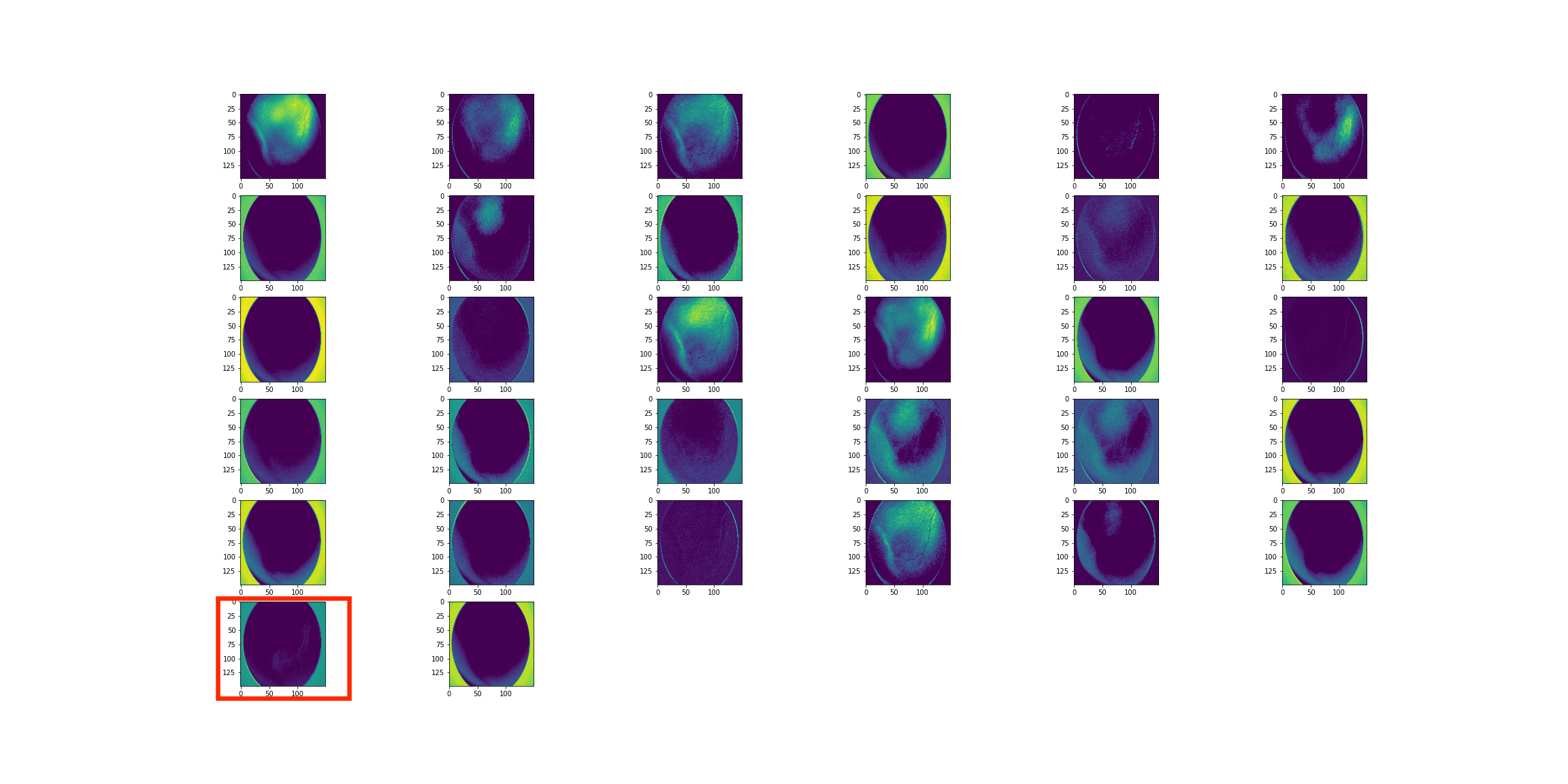
Figure 7: the top left is the preprocessed $300\times 300$ image fed into the ROPBaseCNN; the top right is the extracted feature that shows abnormal blood vessel growth; the bottom is the output from the second layer of ROPBaseCNN.

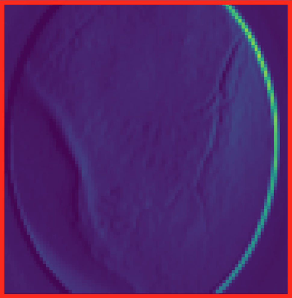
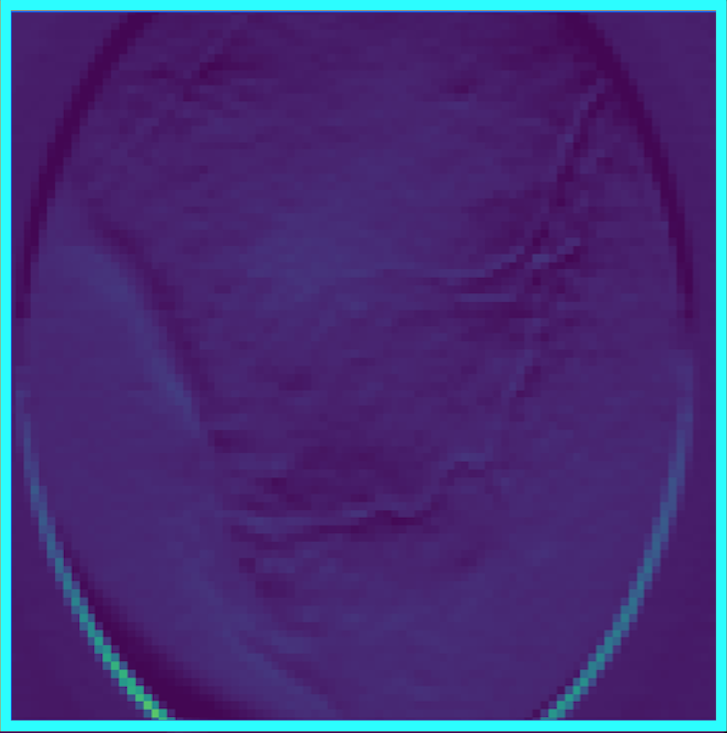
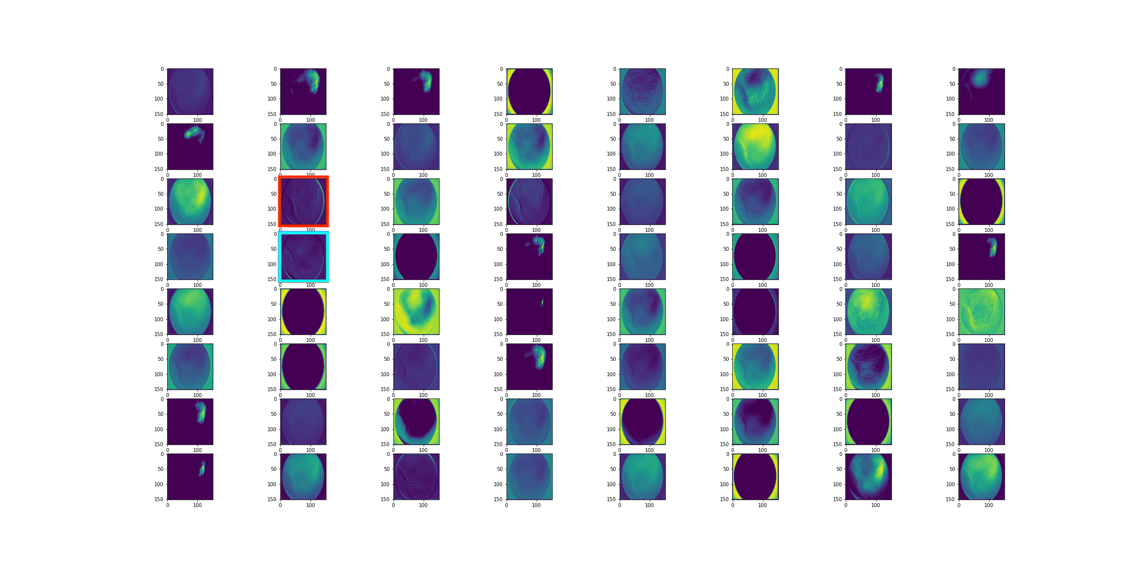
Figure 8: the top left is the preprocessed $300\times 300$ image fed into the ROPResCNN; the top middle and the top right are the extracted features showing the occurrence of the thickened ridge; the bottom is the output from the fifth layer of ROPResCNN.

The architecture of ROPBaseCNN.

For dataset Data_0 with only 2401 samples, complicated models are prone to the overfitting problem on the training data, therefore we first adopt this shallow CNN model with only five layers: two convolution layers and three fully-connected layers. To prevent the issue of overfitting, we add dropout layers [12] in the decoder part and the $L^{2}$ regularization for the kernel of the fully connected layers. The architecture of this shallow CNN, named ROPBaseCNN, is summarized in Figure 4.

Combined with aforementioned data processing strategy, the accuracy of ROP detection under ROPBaseCNN for dataset Data_0 is 93%. This model appears unstable in that its performance would deteriorate with the combined datasets Data_0 and Data_1. (See table 5).

The architecture of ROPResCNN.

The architecture of ROPResCNN combines a pre-trained ResNet50 [8] model (no top) with a global average pool layer and a fully-connected layer as the output layer. The weights of ResNet50 are used as the initial point of the optimization.

With the limited amount of ROP data, training a deep neural network from a random initialization is difficult. Instead, we adopt the pre-trained network weights, which help accelerate the training process because ResNet50 is capable of capturing basic and important features for general image classification. Moreover, with this pre-trained network, we manage to avoid the well-known issues in deep networks such as vanishing/exploding gradient. Additionally, we use the global average pooling at the end of the pre-trained residual network, reducing the dimension from 3D to 1D. Therefore, global pooling outputs one response for every feature map. At the end, a dense layer with one neuron with the Sigmoid activation function aggregates and outputs the probability.

Note that ROPResCNN favors more convolutional layers instead of fully connected ones. With the global-average-pooling for dimension reduction, empirically it is not necessary to add regularization for ROPResCNN.

5 Implementation Results

Data_0 is used in ROPBaseCNN and split into three sets: the training set has 187 positive samples and 990 negative samples, the validation set has 80 positive samples and 425 negative samples, and the testing set has 115 positive samples and 606 negative samples with held-out class labels. A combination of Data_0 and Data_1 is used for ROPResCNN, and is split into three sets: training (431 positive samples and 1216 negative samples), validation (185 positive samples and 521 negative samples), and testing (264 positive samples and 745 negative samples with held-out class labels).

Evaluation metrics.

We use the following standard metrics to evaluate the performance of our models, including precision, sensitivity, specificity, accuracy, and the F1 score,

Precision $$=\frac{TP}{TP+FP},\ \ \ \ \text{Sensitivity}=\frac{TP}{TP+FN},$$

Specificity $$=\frac{TN}{TN+FP},\ \ \ \ \text{Accuracy}=\frac{TP+TN}{TP+TN+FP+FN},$$

F1 $$=2\frac{\text{Precision}\times\text{Sensitivity}}{\text{Precision}+\text{Sensitivity}},$$

where TP, TN, FP, and FN represent true positive, true negative, false positive, and false negative, respectively. The error reduction of the models is calculated as

$$\text{Error reduction}=\frac{\text{human error}-\text{model error}}{\text{human error}}.$$

Training on single GPU.

A single GTX 1080 GPU and 8GB of memory is used for training the ROPBaseCNN-based model and the ROPResCNN-based model. With appropriate data processing, one GPU turns out to be sufficient to fit the training process with 3000 samples per epoch. For ROPBaseCNN, the batch size is 32, and the training is stopped after 25 epochs; for ROPResCNN, the batch size is 64, and the training is stopped after 30 epochs.

Evaluations.

The results of ROPBaseCNN-based model with Data_0 are summarized in the first column of Table 5, the results of ROPBaseCNN-based model with the combined datasets Data_0 and Data_1 are summarized in the second column of Table 5; and the third column shows the results of ROPResCNN-based model with both datasets Data_0 and Data_1.

We take 200 infants’ retinal fundus images with confirmed grading results by ophthalmologists. Their results are then compared against those generated by our models. Figure 6 gives the detailed performance comparison. We see that ROPBaseCNN-based model manages to achieve comparable performance with experienced ophthalmologists, especially in terms of precision and specificity. However, its performance is not robust, with excellent scores from Data_0 vanishing on the combined Data_0 and Data_1.

ROPResCNN-based model dominates both human experts and ROPBaseCNN-model, by a wide margin. It shows impressive performance on the combined Data_0 and Data_1: a perfect score on sensitivity, excellent scores in specificity (96%) and precision (96%), and across-the-board improvement of roughly 10% when compared with experienced ophthalmologists. Most importantly, it reduces human errors by over 66% in all categories, and in particular eliminates completely the error in the category of sensitivity, the most critical requirement for diagnosis of ROP.

Feature map.

The feature map from ROPBaseCNN, shown in Figure 7, captures an implicit indicator of ROP, the abnormal blood vessel growth. However, such a disorder from the retinal fundus image is not used by ophthalmologists as a standard indicator for diagnosis of ROP.

The feature map from ROPResCNN demonstrates that ROPResCNN-based model succeeds in learning and capturing explicitly the well-accepted indicator for the medical diagnosis of ROP: the thickened ridge. (See Figure 8).

6 Summary

Our study shows that models using the state-of-art CNN for general image classification can provide accurate and early detection of ROP with a perfect sensitivity score and excellent scores in specificity and precision. Beyond diagnosis, our study shows that deep neural network techniques can be potentially powerful to extract significant features for better understanding of ROP.

Broader impact

As far as the authors are concerned, a) researchers at the intersection of deep learning and medical imaging can potentially benefit from this work; b) no particular group of people in the society is expected to be put in disadvantage due to this work; c) this work is not subject to the failure of the system; d) data bias is out of the scope of the potential influence of this work; and e) proper understanding of models helps reducing the risk of misdiagnosis.

References

- [1] Hannah Blencowe, Joy Lawn, Thomas Vazquez, Alistair Fielder, and Clare Gilbert. Preterm-associated visual impairment and estimates of retinopathy of prematurity at regional and global levels for 2010. Pediatric research, 74 Suppl 1:35–49, 12 2013.
- [2] Early Treatment For Retinopathy Of Prematurity Cooperative Group. Revised Indications for the Treatment of Retinopathy of Prematurity: Results of the Early Treatment for Retinopathy of Prematurity Randomized Trial. Archives of Ophthalmology, 121(12):1684–1694, 12 2003.
- [3] Walter M. Fierson. Screening examination of premature infants for retinopathy of prematurity. Pediatrics, 142(6), 2018.
- [4] Clare Gilbert, Jugnoo Rahi, Michael Eckstein, Jane O’sullivan, and Allen Foster. Retinopathy of prematurity in middle-income countries. The Lancet, 350(9070):12–14, 1997.
- [5] Varun Gulshan, Lily Peng, Marc Coram, Martin C. Stumpe, Derek Wu, Arunachalam Narayanaswamy, Subhashini Venugopalan, Kasumi Widner, Tom Madams, Jorge Cuadros, Ramasamy Kim, Rajiv Raman, Philip C. Nelson, Jessica L. Mega, and Dale R. Webster. Development and Validation of a Deep Learning Algorithm for Detection of Diabetic Retinopathy in Retinal Fundus Photographs. JAMA, 316(22):2402–2410, 12 2016.
- [6] Guo Haixiang, Yijing Li, Jennifer Shang, Gu Mingyun, Huang Yuanyue, and Bing Gong. Learning from class-imbalanced data: Review of methods and applications. Expert Systems with Applications, 73, 12 2016.
- [7] Mohammad Havaei, Axel Davy, David Warde-Farley, Antoine Biard, Aaron Courville, Yoshua Bengio, Chris Pal, Pierre-Marc Jodoin, and Hugo Larochelle. Brain tumor segmentation with deep neural networks. Medical Image Analysis, 35:18 – 31, 2017.
- [8] Kaiming He, Xiangyu Zhang, Shaoqing Ren, and Jian Sun. Deep residual learning for image recognition. In 2016 IEEE Conference on Computer Vision and Pattern Recognition (CVPR), pages 770–778, 2016.
- [9] Diederik Kingma and Jimmy Ba. Adam: A method for stochastic optimization. International Conference on Learning Representations, 12 2014.
- [10] Yann LeCun, Patrick Haffner, Léon Bottou, and Yoshua Bengio. Object recognition with gradient-based learning. In Shape, Contour and Grouping in Computer Vision, 1999.
- [11] Charles X. Ling and Chenghui Li. Data mining for direct marketing: Problems and solutions. In Proceedings of the Fourth International Conference on Knowledge Discovery and Data Mining, KDD’98, page 73–79. AAAI Press, 1998.
- [12] Nitish Srivastava, Geoffrey Hinton, Alex Krizhevsky, Ilya Sutskever, and Ruslan Salakhutdinov. Dropout: A simple way to prevent neural networks from overfitting. Journal of Machine Learning Research, 15(56):1929–1958, 2014.
- [13] Zhi-Hua Zhou and Xu-Ying Liu. Training cost-sensitive neural networks with methods addressing the class imbalance problem. IEEE Transactions on Knowledge and Data Engineering, 18(1):63–77, 2006.