Cyclical lock-down and the economic activity along the pandemic of COVID-19

Abstract

The investigation focuses on an on-off protocol for controlling the COVID-19 widespread. The protocol establishes a working period of 4 days for all the citizens, followed by 8 days of lock-down. We further propose splitting people into smaller groups that undergo the on-off protocol, but shifted in time. This procedure is expected to regularize the overall economic activity. Our results show that either the on-of protocol and the splitting into groups reduces the amount of infected people. However, the latter seems to be better for economic reasons. Our simulations further show that the start-up time is a key issue for the success of the implementation.

I Introduction

In this investigation we explore a cyclic scheme of isolation (quarantine) and economic activity in order to cope with a pandemic like the Covid-19 one. The proposed scheme consists in a sequence of isolation-activity cycles in which a portion of the population (one third) is fully free to join its usual activities while the other two thirds are subject of the isolation. After four days the third that has been working goes into quarantine (8 days isolation), one of the remaining thirds remains in quarantine and the third one change to a state of full activity. As will be shown this scheme (inspired in Ref. Alon ) allows to properly control the pandemic evolution while keeping the economic cycle active.

The evolution of the disease is performed using a SEIR (Susceptible, Exposed, Infected, Recovered) compartmental model .

In Section II.1 we briefly describe the SEIR model. In Section II.2 we show the way in which the above metioned cyclic alternate scheme is implemented in the 4-8 case.

II The Model

II.1 The SEIR model of a single group

In order to describe the time evolution of a given population when a (small) fraction of it is infected, we resort to the SEIR compartmental model. These kind of models consider that the individuals among the the population can be in one of the following possible states:

• Susceptible individuals, which are not immune to the considered infection, and consequently, can get infected by contact with an infected individual.

• Exposed, is an individual who having been in contact with I, is already a patient but is unable to infect other Susceptible individuals.

• Is the infected state, the individual is able to infect other susceptible individuals.

• Removed state, the individuals in this state do not participate in the process of epidemic evolution any more. It both comprises the individuals who became immune to the illness but also those who die.

In this way this quantities satisfy the following relation

$$S(t)+E(t)+I(t)+R(t)=N$$ (1)

The SEIR model appears as a more accurate model for the coronavirus COVID-19 pandemic with respect to the SIS, SIR, etc.. This is because those individuals who catched the infection undergo an “incubation” period, through which they are not able to infect others.

The equations that describe the evolution of the infection read as follows.

$$\left\{\begin{array}[]{lcl}\dot{s}(t)&=&-\beta i(t)s(t)\\ \dot{e}(t)&=&\beta i(t)s(t)-\sigma e(t)\\ \dot{i}(t)&=&\sigma e(t)-\gamma i(t)\\ \dot{r}(t)&=&\gamma i(t)\end{array}\right.$$ (2)

with $s(t)=S(t)/N$, $e(t)=E(t)/N$, etc. These are the magnitudes per unit individual. For the purpose of simplicity, we will consider $\beta$, $\sigma$ y $\gamma$ as fixed parameters. The parameter $\beta$ (infection rate) represents the effective mean field rate of infection, actuating on the product of the relative susceptible population and the relative infected population. It depends on intrinsic ingredients like the infectivity of the virus under consideration and extrinsic ones like the contact frequency. Besides, the parameters $\sigma$ and $\gamma$ depend exclusively on the illness under consideration.

One of the relevant magnitudes is the so called basic reproduction number $R_{0}$ Dushoff

$$R_{0}=\frac{\beta}{\gamma}$$ (3)

This quantity represents the number of individuals that are infected by a single individual in state I, when interacting with a totally Susceptible population. It is immediate to see that if $R_{0}$ is larger than 1 the infection will blossom. On the contrary, if this quantity is smaller than 1 the infection dies out.

It should be kept in mind that once the process starts developing the $R_{0}$ should be replaced by the $R_{e}$ (i.e. effective reproduction number).

II.2 The SEIR model for three groups and cyclical lock-down

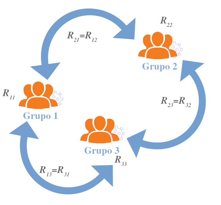
Figure 1: Connectivity scheme for many groups. The disease spreading model corresponds to the SEIR one.

The SEIR model detailed in Section II.1 assumes that the disease spreads over an homogeneous population. However, this may not be the case if some kind of grouping tendency exists among the individuals. The reproduction number may be different within the group, or, between groups. The latter will depend on the isolation degree among the groups. Two completely isolated groups attain independent evolutions. But a small infection leakage povides the mean for the disease propagation from group to group. Fig. 1 represents qualitatively this situation.

A multi-group SEIR model can mathematically represented as follows. Each group is labeled through indexes $i=1...N$. The former (scalar) states S,E,I,R become (column) arrays of states

$$(s_{1},...,s_{N})\,,(e_{1},...,e_{N})\,,(i_{1},...,i_{N})\,,(r_{1},...,r_{N})$$ (4)

respectively. Notice that the total amount of individuals in each state corresponds to the sum of the elements of each array.

Since the propagation can actually occur within each group, or, among them, we define two sets of reproduction numbers. The first set corresponds to the reproduction number within group $R_{ii}=\beta_{ii}/\gamma_{i}$. The second set corresponds to the reproduction number between any two groups $R_{ij}=\beta_{ij}/\gamma_{i}$. The mixing among groups occurs as follows

$${\scriptsize\delta_{ijk}\,s_{k}\beta_{jl}i_{l}=\left(\begin{array}[]{ccc}s_{1}&...&0\\ \vdots&\ddots&\vdots\\ 0&...&s_{N}\\ \end{array}\right)\,\left(\begin{array}[]{c}\beta_{11}i_{1}+...+\beta_{1N}i_{N}\\ \vdots\\ \beta_{N1}i_{1}+...+\beta_{NN}i_{N}\\ \end{array}\right)}$$ (5)

for $\delta_{ijk}$ representing the Kronecker tensor and $i,j,k,l=1,...,N$. The whole set of equations read

$$\left\{\begin{array}[]{lcl}\dot{s}_{i}(t)&=&-\delta_{ijk}\,\beta_{jl}\,s_{k}(t)\,i_{l}(t)\\ &&\\ \dot{e}_{i}(t)&=&\delta_{ijk}\,\beta_{jl}\,s_{k}(t)\,i_{l}(t)-\sigma_{ij}\,e_{j}(t)\\ &&\\ \dot{i}_{i}(t)&=&\sigma_{ij}\,e_{j}(t)-\gamma_{ij}\,i_{j}(t)\\ &&\\ \dot{r}_{i}(t)&=&\gamma_{ij}\,i_{j}(t)\\ \end{array}\right.$$ (6)

for $\sigma_{ij}=\mathrm{diag}(\sigma_{11},...,\sigma_{NN})$ and $\gamma_{ij}=\mathrm{diag}(\gamma_{11},...,\gamma_{NN})$ (meaning that $\sigma_{ij}$ and $\gamma_{ij}$ are diagonal matrices).

III Simulations

We implemented the Runge Kutta 4th-order method in order to integrate the differential equations. The chosen time step was 0.1 (days).

As mentioned in Section II, the parameters $\sigma$ and $\gamma$ represent the incubation rate and the recuperation rate, respectively. Therefore, $\sigma^{-1}$ and $\gamma^{-1}$ correspond to the mean incubation time and the mean recovering time, respectively. According to preliminary estimations for COVID-19, we consider the following parameter values for the SEIR model: $\sigma^{-1}=3\,$days and $\gamma^{-1}=4\,$days Milo ; oms ; hopkins ; Lessler .

The cyclical work-lockdown implementation

We first implemented a cyclic work-lockdown strategy in the same way as in Ref. Alon . This one corresponds to a cyclical schedule of lock-down and work days. As already mentioned in Section II, ​the transmission parameter $\beta$ is the only parameter to be modified through lockdown policies. Recall that this parameter depends on the number of individual contacts. Therefore, policies like lock-down can reduce its value, and thus, the value of $R_{0}$ (see Eq. 3).

The cyclical work-lockdown strategy corresponds to $W$-days of work and $L$-days of lock-down $(W,L)$. Two transmission parameters ($\beta$) may be accomplished on each period, due to the different number of contacts. These are $\beta_{W}$ for the working days and $\beta_{L}$ for the lock-down days, with the associated reproduction numbers $R_{W}$ and $R_{L}$, respectively (see Eq. 3). We assume $R_{L}\leavevmode\nobreak\ =\leavevmode\nobreak\$0.6 and $R_{W}\leavevmode\nobreak\ =\leavevmode\nobreak\$1.5 (or greater) as in Ref. Alon .

IV Results

In this section we discuss the results obtained. We divided our investigation into two different scenarios. We first examined the case in which there is no intervention during the pandemic (Section IV.1), while the intervention case is left to Section IV.2.

IV.1 The uncontrolled pandemic spreading

As a first step we examined how the pandemic spreads without any kind of intervention. In other words, withouth any cyclical strategy. According to Ref. Milo , we assumed that the reproduction number is 3. Fig. 2 shows the evolution of the susceptible, exposed, infected and recovered individual along time. As can be seen, the number of susceptible individuals decreases monotonically during time. On the contrary, an opposite behavior can be observed for the recovered individuals. In this case, they increase monotonically along time.

Besides, Fig. 2 shows that the exposed and infected individuals adopt a similar profile. As can be seen, the peak of infected individuals is reached at the fifth week. The height and width of the infected peak depends on the value of $R_{0}$. Thus, the greater the value of $R_{0}$, the higher the peak. And, in turn, narrower.

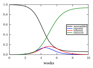
Figure 2: Pandemic evolution. We used $\sigma^{-1}=3\,$days, $\gamma^{-1}=4\,$days and $\beta=$0.75 ($R_{0}$=3) Milo . The initial condition was $s(0)=1,s(0)=0,i(0)=1\times 10^{-3}$ y $r(0)=0$.

IV.2 Evolution of the pandemic with cyclical strategy

We now discussed the effects of applying the lockdown-work cycle during the pandemic. We will use the term homogeneous group to define a set of individuals that is in a single state. That is, a homogeneous group is one that is in a state of “lockdown” or “work”, but not both. Two possible scenarios will be analyzed below:

• An unique homogeneous group: there is only one homogeneous group.

• Three homogeneous groups (multi-group): the crowd is divided into three groups of individuals of the same size. People in each group interact with those in the same group ($R_{ii}$). Also, people from one group can interact with people from another group ($R_{ij}$). It should be noted that, in this case, one group may be in a state of “lockdown”, while the other two groups in a state of “work” or “normal activity”.

IV.2.1 The (4-8) and (4-10) cycles for a single group

Fig. 3 shows the number of infected individuals when we apply the lockdown-activity strategy for two different schedules (4-8 days and 4-10 days). Notice that this is applied after the number of infected surpasses $10\%$ of the total population. We compare this evolution with respect the case in which a permanent lockdown is applied (see Fig. 3). As can be seen, in both cases, the best strategy in terms of the number of infected people, is a continuous (or strict) lock-down. In this case there is a monotonically decrease in the number of infected over time.

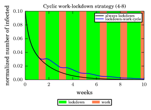
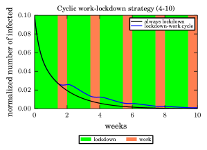
Figure 3: Normalized number of infected individuals along time. The initial condition was $s(0)=0.9,s(0)=0,s(0)=0.1$ and $s(0)=0$. The reproduction number for the “always lockdown” was $R_{l}=0.6$. On the other hand, in the “lockdown-work cycle” we used $R_{w}=1.5$ and $R_{l}=0.6$.

We can further see in Fig. 3 that when applying the cyclical strategy (blue line) there is an increase in the number of cases due to the inclusion of the “activity” stage (equivalent to the release of the lock-down). In this sense, we can see that during this stage (see orange bars) the number of infected grows, unlike what happens in the “lock-down” stage (green bars).

Finally, we can observe a similar behavior when applying cycles (4-8) and (4-10) in terms of the number of infected. It should be noted that similar results are obtained in the case of the susceptible, exposed and recovered (not shown). Thus, we conclude that applying a cycle (4-8) is similar to the schedule (4-10). However, as we will see below, the first case allows us a continuous cycle of “activity” if three groups of individuals are considered.

In the next section we will focus on the study of the cycle (4-8).

IV.2.2 Analysis of the (4-8) estrategy for a single group

Unlike the previous case, we now analyze the effects of applying the lockdown-activity cycle during different stages of the pandemic. Fig. 4 shows the evolution of each stage (susceptible, exposed, infected and recovered) as a function of time. We also plotted the case in which the system is allowed to evolve freely, equivalent to a “continuous activity” (red line). Starting from this curve, we applied the lockdown-activity cycle at different times of the evolution (see black lines).

As can be seen in Fig. 4, the number of susceptible people decreases monotonically along time due to the progressive spreading of the virus. Also, we can note that once the lockdown-activity cycle has been implemented, the number of susceptible people reaches, seemengly in four weeks, an asymptotic regime. The same occurs with the recovered individuals (see Fig. 4(d)), but in this case they increases monotonically with time.

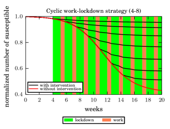
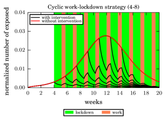
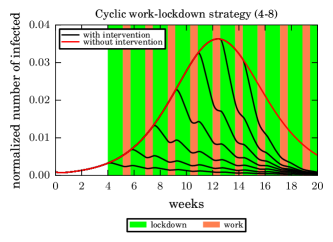
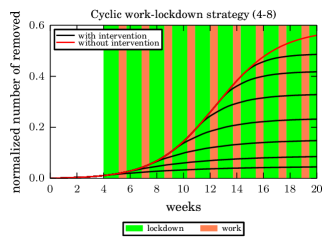
Figure 4: Normalized number of susceptibles (a), exposed (b), infected (c) and recovered (d) as a function of time. The initial condition was $s(0)=1,e(0)=0,i(0)=1\times 10^{-3}$ y $r(0)=0$. The $R$ numbers for the intervention scenario were $R_{w}=1.5$ and $R_{l}=0.6$, while for “non-intervention” $R_{0}=$1.5.

Notice that the behavior of the number of susceptibles and recovered individuals is not affected by the start-up time. That is, the number of susceptibles decreases monotonically regardless of whether the population is in the lock-down or activity stage (the same occurs in the case of those recovered). However, we can observe a completely different behavior in the case of the exposed and the infected individuals. In this case, we can see that their behavior is affected according to the time of the evolution. Notice that the number of exposed individuals grows during the “activity” stage. This can be explained if we take into account that during the “activity” stage, the frequency of contacts between susceptibles and infected increases (through $R_{w}$). Therefore, increases the probability of transmitting the virus to a susceptible. If this happens, the susceptible becomes to an exposed one. The opposite occurs in the lock-down stage, where there is a lower probability to transfer the virus.

Interesting, Fig. 4 also shows that the behavior of the number of infected individuals during the “activity” stage depends on the time of the intervention. That is, we can observe that, before week 11, the number of infected increases during the “activity” stage. Instead, this behavior is reversed (decreases) from, approximately, this point. So, the return to the activity stage does not affect the system in terms of an increase in the number of infected. Furthermore, it should be noted that this occurs before reaching the peak of the epidemic.

Up to now, we have analyzed how the epidemic evolves when considering a single homogeneous group, which can adopt a “lock-down” or “activity” behavior. In the next Section we consider three groups of individuals. As previously mentioned, this case allows optimizing the strategy (4-8).

IV.2.3 Analysis of the (4-8) strategy for three groups

We now focus on the population that appears splitted into three groups $i=1,2,3$. Recall that each group cycles through a normal working period and a lock-down period. The lock-down period fits into the mean time of the infection (say, $L=8$), while the working period lasts for approximately a working week ($W=4$). These $4\times 8$ periods for each group are set shifted in time, according to the schedule in Fig. 5.

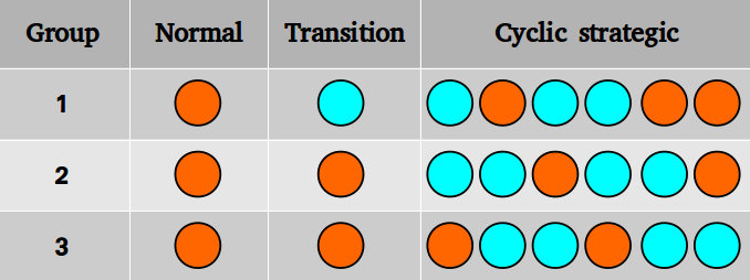
Figure 5: Schedule for the cycical estrategy on three groups. The orange and blue circles represent the working period and the lock-down period, respectively. The “normal” column means no estrategy at all. The column “transition” attains for the required shifting before the $4\times 8$ strategy is fulfilled.

The reproduction number within each group is $R_{ii}=\beta_{ii}/\gamma_{ii}$. We assume two possible situations: normal working activity with $R_{ii}=R_{w}>1$, or, the lock-down situation with $R_{ii}=R_{l}<1$. We further assume two possible reproduction values between the groups: a complete isolation ($R_{ij}=0$, $i\neq j$) or some leakage among them ($R_{ij}\ll 1$, $i\neq j$).

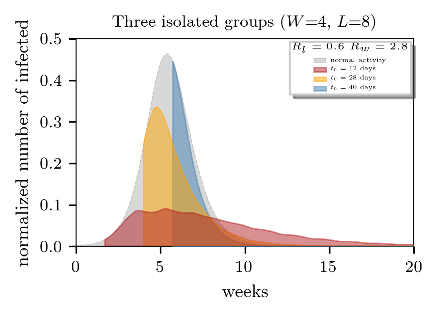
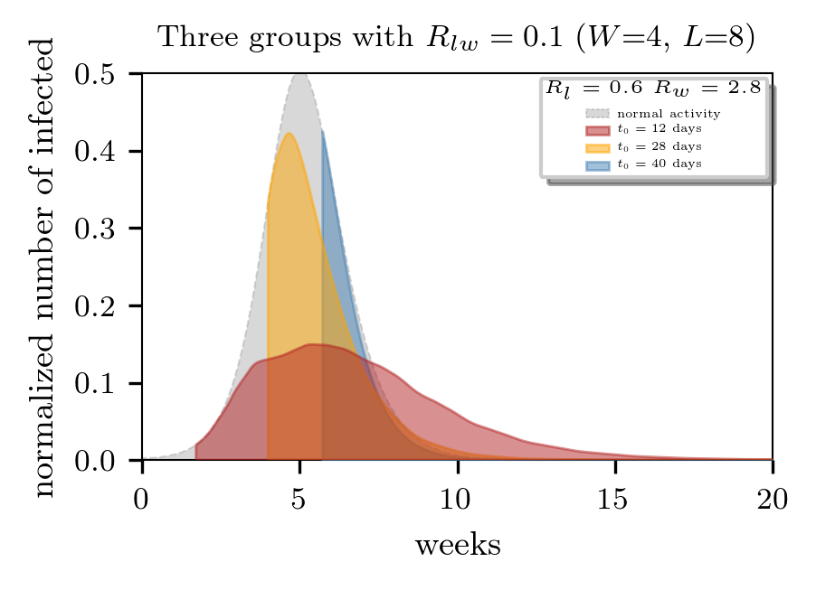
Figure 6: Total number of infected people ($i_{1}+i_{2}+i_{3}$) vs. time. The initial conditions are $s(0)=1,e(0)=0,i(0)=1\times 10^{-3}$ and $r(0)=0$. The reproduction numbers for the “normal working” and the “lock-down” situations are $R_{w}=2.8$ and $R_{l}=0.6$, respectively. The working days are $W=4$, while the lock-down days are $L=8$. (a) The three groups are completely isolated ($R_{ij}=0$). (b) An infection leak exists between the group ($R_{ij}=0.1$).

Fig. 6 shows the time evolution for the total infected people for either isolated groups and non-insolated ones (see caption for details). The area in gray corresponds to the natural evolution with no strategy at all. The red, orange and blue colors correspond the $4\times 8$ strategy (see caption for details). The strategy start-up date is indicated in the legend.

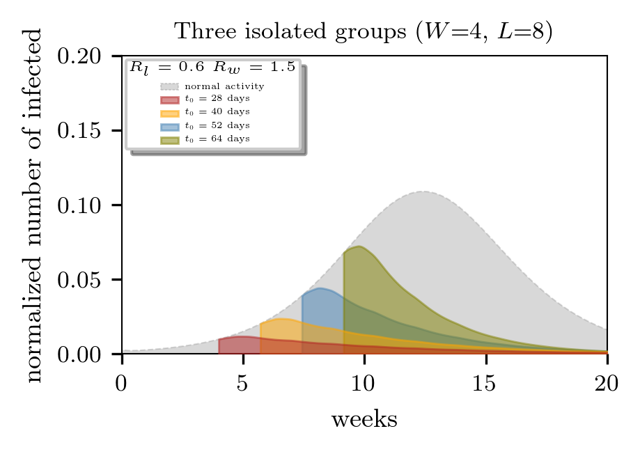
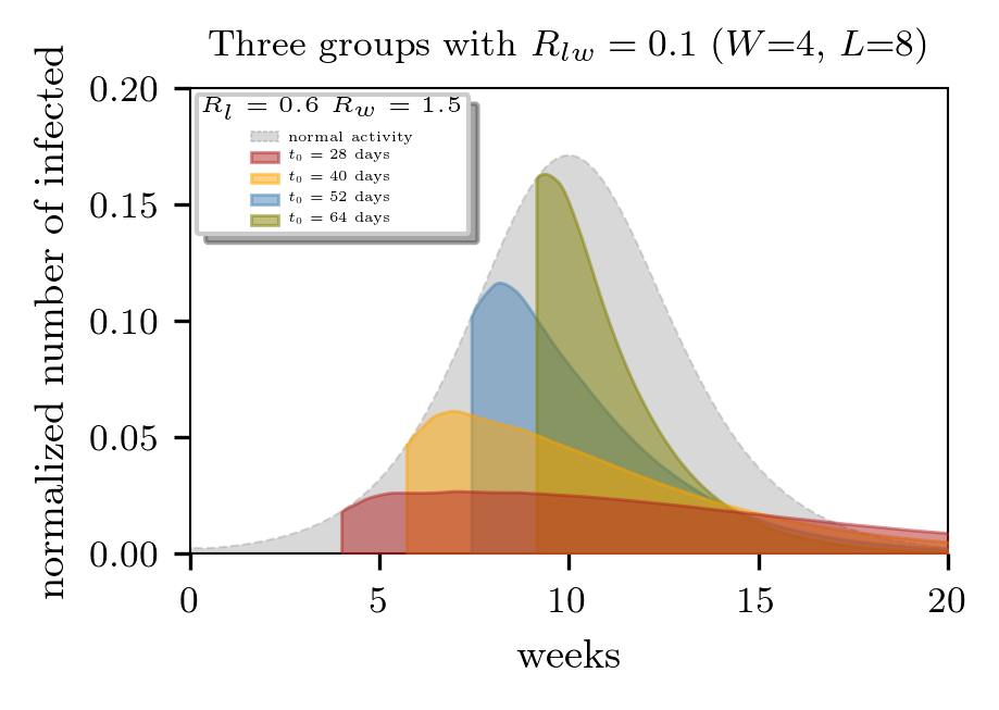
Figure 7: Total number of infected people ($i_{1}+i_{2}+i_{3}$) vs. time. The initial conditions are $s(0)=1,e(0)=0,i(0)=1\times 10^{-3}$ and $r(0)=0$. The reproduction numbers for the “normal working” and the “lock-down” situations are $R_{w}=1.5$ and $R_{l}=0.6$, respectively. The working days are $W=4$, while the lock-down days are $L=8$. (a) The three groups are completely isolated ($R_{ij}=0$). (b) An infection leak exists between the group ($R_{ij}=0.1$).

The cyclical strategy decreases the amount of infected people as the process evolves, regardless of the infection leak among groups. However, if the groups remain completely isolated, the strategy exhibits a better performance. Besides, late implementation of the strategy provides poor results.

Fig. 7 shows similar results as in Fig. 6, but for a weaker reproduction number. Notice that both scenarios decrease the total number of infected people. Thus, the $4\times 8$ strategy can be applied to a variety of infectious diseases (that is, different $R$).

V Conclusions

We studied the time evolution of an infection describable by a SEIR compartmental model. Specifically, we implemented a cyclical asymmetric scheme by which the total population is divided in 3 parts, each performing a 4 days normal activities period and an 8 days isolation period. This sequence is performed by each group comprising a third of the population in such a way that, at any given time, one third of the population is performing their usual “normal” duties. In this way the solution of the SEIR equations indicate that the disease can be controlled while keeping a sensible degree of economical activity.