A novel approach to chemotaxis: active particles guided by internal clocks

Abstract

Motivated by the observation of non-exponential run-time distributions of bacterial swimmers, we propose a minimal phenomenological model for taxis of active particles whose motion is controlled by an internal clock. The ticking of the clock depends on an external concentration field, e.g. a chemical substance. We demonstrate that these particles can detect concentration gradients and respond to them by moving up- or down-gradient depending on the clock design, albeit measurements of these fields are purely local in space and instantaneous in time. Altogether, our results open a new route in the study of directional navigation, by showing that the use of a clock to control motility actions represents a generic and versatile toolbox to engineer behavioral responses to external cues, such as light, chemical, or temperature gradients.

In the canonical picture of bacteria with run-and-tumble motility, such as Escherichia coli or Salmonella Berg and Brown (1972); Berg (2008), bacteria display exponentially distributed run-times – despite recent findings that suggest the possibility of noise-induced heavy-tailed distributions Korobkova et al. (2004); Tu and Grinstein (2005) – and perform chemotaxis by regulating the associated tumbling frequency. By measuring the chemical concentration through clustered arrays of membrane receptors Tindall et al. (2012) and subsequent signal processing via a complex biochemical cascade Celani and Vergassola (2010) that leads to an effective memory Schnitzer (1993); Celani and Vergassola (2010); Cates (2012); Flores et al. (2012), the bacterium is able to detect and respond to an external concentration gradient. It extends the duration of runs, i.e. decreases the number of tumbles when heading in the direction of increasing attractant concentration, thus performing a biased random walk towards the attractant source. Recently, it was discovered that several bacterial species differ from this classical picture. Notably, in the soil bacterium Pseudomonas putida (P. putida) that displays a run-and-reverse motility pattern with multiple run modes Hintsche et al. (2017); Alirezaeizanjani et al. (2020), the distribution of run-times is non-exponential and exhibits a refractory period, cf. Fig. 1a and Refs. Theves et al. (2013, 2015); an observation that suggests that run-times are not controlled by a Poissonian mechanism . By adapting the reversal statistics in response to a chemical gradient, P. putida is able to perform chemotaxis as indicated in Fig. 1b. However, the non-exponential run-time distribution suggests that chemotaxis in P. putida, and potentially also in other bacterial species, may involve a taxis mechanism that is fundamentally different from the one reported for E. coli. Similar non-exponential bell-shaped run-time distributions were reported for Myxococcus xanthus Wu et al. (2009) and Paenibacillus dendritiformis Be’er et al. (2013), which display run-and-reverse motility similar to P. putida. Non-exponential run-times were observed also for the marine bacterium V. alginolyticus Xie et al. (2011) and, notably, also for the rotation time of the flagellar motors of Escherichia coli Korobkova et al. (2006). Furthermore, it has been reported that surface exploration of Escherichia coli Ipiña et al. (2019) is not consistent with the canonical run-and-tumble picture of bacterial motility, but involves multiple motility modes.

Motivated by the non-Poissonian run-time statistics of P. putida – though not pretending to be a realistic, biochemical description of chemotaxis in P. putida – we propose a minimal, phenomenological, generic model for taxis of active particles that inherently produces non-exponential run-time distributions. Particles move at constant speed and experience velocity reversals. The key element of the model is that the occurrence of reversal events is controlled by an internal clock. The clock mimics the fact that the directional response of a microorganism to an external signal or field, such as a chemical concentration or temperature gradient, requires to sense this signal, internalize and process it, presumably involving cascades of biochemical events Korobkova et al. (2006); Wang et al. (2017), and to execute a behavioral response (e.g. a reversal), after which the microorganism continues sensing, processing and responding to the signal. We assume that this complex cycle can be reduced to a series of stochastic checkpoints or steps, where some or all of them depend on the external signal. These steps are represented by the “ticks” of a clock. The transitions between two consecutive ticks are modeled as Poissonian processes with concentration-dependent transition rates. Ergo, the clock dynamics is, by definition, Markovian: it does not incorporate or presuppose memory in any manner. On the other hand, the distribution of the times between two consecutive behavioral responses is non-exponential as observed in P. putida experiments, cf. Fig. 1a. Experimental details on cell culturing, the chemotaxis chamber and imaging can be found in the Supplemental Material (SM) and Refs. Sambrook and Russell (2001); Harwood et al. (1990, 1984); Pohl et al. (2017); Theves et al. (2013).

In this study, we demonstrate that the design of the clock controls the long-time motility of the particles: some of the clock designs result in signal-insensitive particles and a variety of other designs lead to particles displaying actual taxis. The taxis responses include either up-gradient or down-gradient biased motion. In short, we show how a clock can be used to guide active particles subjected to external stimuli, and to obtain non-exponential run-time distributions.

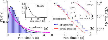
Figure 1: Run-time distribution and chemotactic response of P. putida. Left: probability distribution function (PDF) $\phi$ of run times. Right: cumulative distribution function (CDF) of run-times discriminating between up-gradient ($\Phi_{u}$) and down-gradient ($\Phi_{d}$) runs. The purple-dashed and black-solid curves in the left panel correspond to fittings with an exponential and a $\gamma$-distribution, respectively. A $\chi^{2}$-test indicates that an exponential distribution is rejected at significance level $0.05$. The insets show that the same qualitative behavior is obtained in simulations with a clock model as introduced in the main text. Parameters: $M=2$, $\gamma_{1}=5\,\mbox{s}^{-1}$, $\gamma_{2}(x)=[0.75(x/L)+0.1]^{-1}\mbox{s}^{-1}$, $L=750\,\mu\mbox{m}$ and $v_{0}=30\,\mu\mbox{m}/\mbox{s}$.

Model

We consider active particles that move at constant speed $v_{0}$ in a one-dimensional system of size $L$ with reflecting boundary conditions. Particles are exposed to a temporally constant external field $c(x)$. The equation of motion of one of these particles is given by

$$\frac{dx(t)}{dt}=v(t)=v_{0}s(t),$$ (1)

where $x(t)$ denotes the position of the particle and $s(t)\in\{-1,1\}$ indicates its direction of motion. The variable $s(t)$ undergoes stochastic transitions such that $s(t)\!\to\!-s(t)$. These reversal events are controlled by a stochastic $M$-tick clock. A reversal occurs every time the clock completes a full cycle, i.e. in the transition from $M$ to $1$, as illustrated in Fig. 2. Thus, the state of a particle is characterized by its position $x(t)$, its orientation $s(t)$ as well as the internal state (or tick) of the clock $n\!\in\!\{1,2,\dots,M\}$.

Clock dynamics

The transition between tick $n$ to $n+1$ is modeled by a Poisson process with a concentration dependent transition rate $\gamma_{n}\!\left(x\right)=f_{n}[c(x)]$, where the function $f_{n}[c]$ denotes the dependence of the $n$-th rate on the external field $c(x)$. For simplicity, we will henceforth denote the rates as functions of $x$, keeping in mind, however, that the dependence arises via the gradient in $c(x)$. If all transition rates are independent of the external field $c(x)$ and equal, i.e., $\gamma_{n}=\beta$ with a positive constant $\beta$, the spatially homogeneous case studied in Großmann et al. (2016) is recovered. It is important to notice that the model can be easily formulated in two dimensions as explained in the SM, however, we focus on the one-dimensional scenario for simplicity and without loss of generality here. Let $P_{n}(t)$ denote the probability to find the clock in state $n$ at time $t$. The temporal evolution of $P_{n}(t)$ can be expressed via the Master equation Gardiner (2010)

$$\frac{dP_{1}(t)}{dt} =-\gamma_{1}\!\!\>\big{(}x(t)\big{)}P_{1}\!\left(t\right)+\gamma_{M}\!\!\>\big{(}x(t)\big{)}P_{M}(t)$$ (2a)

$$\frac{dP_{n}(t)}{dt} =-\gamma_{n}\!\!\>\big{(}x(t)\big{)}P_{n}(t)+\gamma_{n-1}\!\!\>\big{(}x(t)\big{)}P_{n-1}(t)$$ (2b)

with $n\!\in\!\left\{2,3,\dots,M\right\}$. Notice that this is a closed chain of states.

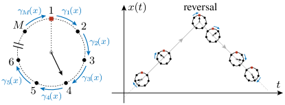
Figure 2: Illustration of the internal clock dynamics (left panel) and the resulting particle motion (right panel). The transition rates $\gamma_{n}\!\left(x\right)=f_{n}[c(x)]$ may be concentration dependent. A particle reverses its direction of motion, i.e., $s(t)\rightarrow-s(t)$, after a full clock cycle has been completed as indicated by a red square on the clock. A segment of a space-time trajectory is represented by a gray line in the right panel. Additionally, the internal dynamics is overlaid at those instances in time in which clock ticks occur.

Run-time distribution

To compute the run-time distribution, we solve for the first passage time of a directed walk from state $1$ to state $M$ within the clock. Let us consider a particle that moves in direction $s_{0}$ at time $t_{0}$ and is in state $1$. We follow its dynamics in space given by $x\!\left(t\right)\!=\!x_{0}\!+\!s_{0}v_{0}(t-t_{0})$ and stop it when it leaves state $M$. We can obtain the probabilities $P_{n}(t)$ by recursion:

$$\!\!P_{1}\!\left(t\right) \!=\!e^{-\!\int_{t_{0}}^{t}dt^{\prime}\gamma_{1}\!\!\>\left(x(t^{\prime})\right)}\!\!\>,\!\!$$ (3a)

$$\!\!P_{n}\!\left(t\right) \!=\!\!\int_{t_{0}}^{t}\!dt^{\prime\prime}\gamma_{n-1}\!\!\>\big{(}x(t^{\prime\prime})\big{)}P_{n-1}\!\left(t^{\prime\prime}\right)e^{-\!\int_{t^{\prime\prime}}^{t}dt^{\prime}\gamma_{n}\!\!\>\left(x(t^{\prime})\right)}\!\!\>.\!\!$$ (3b)

The run-time distribution is given by $\phi(t|x_{0},s_{0})\!=\!\gamma_{M}\big{(}x(t)\big{)}P_{M}(t)$; an example of $\phi$ for a $M=2$ clock is shown in Fig. 1.

Spatio-temporal dynamics

Since we are dealing with a genuine Markov process, the exact, full spatio-temporal dynamics of the problem can be described in terms of a Master equation for the probability density $P_{n}^{\pm}\!\left(x,t\right)$ to find a particle in position $x$ at time $t$ oriented along the direction $s\!=\!\pm 1$ with the internal state $n$:

$$\Big{[}\partial_{t}\!\pm\!v_{0}\partial_{x}\!\!\>\!+\!\gamma_{n}\!\left(x\right)\!\Big{]}\!P_{n}^{\pm}\!\left(x,t\right) \!=\!\begin{cases}\!\>\!\gamma_{M}\!\left(x\right)\!P_{M}^{\mp}\!\left(x,t\right)\!,&\!\!\!\!n=1,\\ \!\>\!\gamma_{n-1}\!\left(x\right)\!P_{n-1}^{\pm}\!\left(x,t\right)\!,&\!\!\!\!n\geq 2.\end{cases}$$ (4)

This is a system of $2M$ coupled linear partial differential equations. Notice that the dynamics of $P_{1}^{\pm}\!\left(x,t\right)$ is special since it contains the dynamics of reversals. Eq. (4) can be expressed in a concise matrix form for the vector

$$\mathbf{P}\!\left(x,t\right)=\left(P_{1}^{+}\!\left(x,t\right)\!,P_{1}^{-}\!\left(x,t\right)\!,\dots,P_{M}^{+}\!\left(x,t\right)\!,P_{M}^{-}\!\left(x,t\right)\right)^{\!T}$$

as follows:

$$\partial_{t}\mathbf{P}\!\left(x,t\right)=\mathcal{C}\cdot\partial_{x}\mathbf{P}\!\left(x,t\right)+\mathcal{L}(x)\cdot\mathbf{P}\!\left(x,t\right)\!,$$ (5)

where the matrix $\mathcal{C}$, which encodes the motility of particles, is diagonal with the coefficients $\mathcal{C}_{ij}\!=\!(-1)^{j}v_{0}\delta_{ij}$ and $\mathcal{L}\!\left(x\right)$ contains the transition rates of the clock dynamics as well as the reversals. The time-dependent solution may be written as $\mathbf{P}\!\left(x,t\right)\!=\!\exp\left[\left(t-t_{0}\right)\!\mathcal{M}\!\left(x\right)\right]\!\mathbf{P}\!\left(x,t_{0}\right)$, where we introduced the operator $\mathcal{M}\!\left(x\right)\!=\!\mathcal{C}\partial_{x}\!+\!\mathcal{L}\!\left(x\right)$ on the right hand side and $\mathbf{P}\!\left(x,t_{0}\right)$ abbreviates the initial condition Risken (1996).

Clock design & taxis response

If there is an observable taxis response, the density $\rho(x,t)=\sum_{n=1}^{M}\left[P_{n}^{+}(x,t)+P_{n}^{-}(x,t)\right]$ to find a particle at position $x$ should be spatially modulated in the long time limit, i.e., $\rho(x)=\lim_{t\to\infty}\rho(x,t)$ should not be constant. We exploit the fact that the time-independent solution of the Master equation (4) is unique Van Kampen (2011). In this way, we can easily verify whether a non-constant $\rho(x)$ should be expected for a given clock design.

We classify clock designs into two categories, homogeneous and inhomogeneous clocks, addressed separately in the following.

(1) Homogeneous clocks: We call a clock homogeneous if all transition rates $\gamma_{n}(x)$ are identical functions of the concentration: $\gamma_{n}\!\left(x\right)\!=\!f[c\!\left(x\right)]$ for $n=1,2,\dots,M$ with an arbitrary function $f[c]$. We start by considering a special case of great relevance: a clock model with only one tick ($M=1$). In this particular case, the Master equation reduces to

$$\Big{(}\!\!\>\partial_{t}\pm v_{0}\partial_{x}\!\!\>\Big{)}\!\>\!P_{1}^{\pm}\!\left(x,t\right)=\gamma_{1}(x)\Big{[}P_{1}^{\mp}\!\left(x,t\right)-P_{1}^{\pm}\!\left(x,t\right)\!\!\>\Big{]}.$$ (6)

Even though the transition rate $\gamma_{1}$ depends on $c(x)$, the stationary solution is spatially independent: $P_{1}^{\pm}\!\left(x\right)\!=\!(2L)^{-1}$. In short, a particle moving at constant speed is unable to detect a chemical gradient if the reversal process is controlled by a Poisson process ($M=1$) with a concentration dependent transition rate. Surprisingly, a homogeneous stationary solution, $P_{n}^{\pm}\!\left(x\right)\!=\!\left(2ML\right)^{-1}$, is also obtained for all homogeneous clocks with $M>1$, despite the run-time distributions are $\gamma$-shaped.

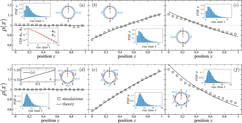
Figure 3: Stationary distributions $\rho(x)$ for two homogeneous, $(a)$ and $(d)$, and four inhomogeneous clocks, $(b)$,$(c)$, $(e)$ and $(f)$, with $M=2$ and $M=5$ internal states. Points represent particle-based simulations and lines show the density profiles as predicted by the perturbation theory. The external field $c(x)$, common for all cases shown, is displayed as an inset in panel (d). If all rates are equal (homogeneous clocks), a uniform density profile develops – particles are thus unable to respond to the chemical gradient [panels $(a)$ and $(d)$]. However, there can be a run-time bias, calculated from Eq. (3) as indicated in the inset of panel $(a)$. A nonuniform density profile is observed if the symmetry of the internal dynamics is broken. The probability to find a particle is proportional to the modulation of the first transition rate $\alpha(x)$ [panels $(b)$ and $(e)$]. By inverting the design of the clock [panels $(c)$ and $(f)$], the gradient in the resulting density profile switches sign with respect to the former case. For all cases, the run-time distribution $\phi(t)$ (shown in each panel as an inset using the same bin width of $\Delta t=0.7$) is bell-shaped when there is more than $M=1$ internal state. Note that the shape of the run-time distribution as well as the steepness of the density gradient depend on the design of the clock. Parameters in arbitrary units: $\alpha(x)\!=\!c(x)$, $c(x)=0.75+0.5x$, $\beta=1$, $v_{0}=0.01$, $L=1$. For particle-based simulations, $N=10^{4}$ particles were simultaneously tracked using a stochastic Euler scheme Gardiner (2010) with $\Delta t=10^{-3}$ and density distributions were averaged over time neglecting initial transients.

We stress that homogeneous clocks will, however, lead to a measurable run-time bias at the single particle level, i.e. run-times up-gradient differ compared to their down-gradient counterparts, cf. the inset in Fig. 3a and Eq. (3). Nevertheless, there is no accumulation at concentration maxima nor minima. In short, homogeneous clocks with multiple ticks do not induce a long-time taxis response as illustrated in Fig. 3a,d. We thus conclude that the measurement of stationary concentration profiles is an indispensable piece of information, whereas the observation of a run-time bias in the individual trajectories provides only insufficient insight into the long-time chemotaxis performance.

(2) Inhomogeneous clocks: If at least two transition rates are different from one another, the stationary state is not spatially homogeneous and nontrivial stationary profiles of $\rho(x)$ can develop (see Fig. 3b,c,e, and f). For arbitrary spatial dependencies of the transition rates $\gamma_{n}(x)$, we cannot find the exact stationary solution of Eq. (4) analytically, but various approximation methods can be applied.

In Ref. Nava et al. (2018), a drift-diffusion approximation of the Fokker-Planck type Gardiner (2010)

$$\partial_{t}\rho\!\left(x,t\right)\simeq-\partial_{x}\Big{[}f(x)\rho\!\left(x,t\right)\Big{]}\!+\partial_{x}^{2}\Big{[}D(x)\rho\!\left(x,t\right)\Big{]}$$ (7)

for the long-time dynamics of the density $\rho(x,t)$ was proposed in a related context, derived under the assumption that the mean distance traversed by a particle in between two reversals is shorter than the characteristic length scales at which the chemical gradient varies. The approximation scheme is based on a slow mode reduction of the full Master equation [Eqs. (4)]: as the particle density $\rho(x,t)$ is a conserved quantity, its dynamics is slow, thus enabling the systematic adiabatic elimination of fast degrees of freedom. In this way, drift $f(x)$ and diffusion $D(x)$ can be analytically obtained for any clock motif Nava et al. (2018). This approximation allows the prediction of the density profile $\rho(x)$ in the long-time limit based on the stationary solution of Eq. (7).

In this work, we present a perturbative approach that enables us to predict the stationary solution for the vector $\mathbf{P}(x)$ including all of its components beyond the scalar, stationary density $\rho(x)$. In Figs. 3 and 4, we compare particle-based simulations with the perturbative solution whose derivation is sketched below (see SM for additional technical details). The central idea of the perturbation theory is that the transition rates are only weakly modulated in space allowing us to split the matrix $\mathcal{L}\!\left(x\right)$ into a constant and a spatially dependent part, $\mathcal{L}\!\left(x\right)\!\!=\!\mathcal{L}_{0}\!+\!\varepsilon\mathcal{L}_{\Delta}\!\left(x\right)$, where the second matrix is defined in such a way that $\int_{0}^{L}dx\,\mathcal{L}_{\Delta}\!\left(x\right)\!=\!0$. Now, we assume that $\varepsilon$ is a small parameter allowing to expand the stationary solution as a power series: $\mathbf{P}\!\left(x\right)\!=\!\sum_{n=0}^{\infty}\mathbf{P}_{\mu}\!\left(x\right)\varepsilon^{\mu}$. Inserting this ansatz into Eq. (5) and collecting orders in $\varepsilon$ yields a systematic way to construct the stationary solution. This approach allows us to demonstrate (i) that active particles controlled by inhomogeneous clocks display a taxis response and (ii) how the clock design determines the type of response. Figures 3b and 3c show the emerging density profiles for particles with $M=2$-clocks subjected to the same external field, where the transition rates are $\gamma_{1}=\alpha(x)$ and $\gamma_{2}=\beta$ in Fig. 3b, while $\gamma_{1}=\beta$ and $\gamma_{2}=\alpha(x)$ in Fig. 3c. The important observation here is that $\rho(x)$ increases monotonically for the former clock and decreases for the latter one as one moves in up-gradient direction with respect to $c(x)$; notably, the average tumbling frequency increases in both cases in the up-gradient direction. In Fig. 3e and 3f, a similar scenario is shown for an $M=5$-clock for comparison. While the qualitative trends remain the same, the gradient in the nonuniform density profiles becomes steeper in the $M=5$-case.

In Fig. 4, a detailed comparison of individual-based simulations and the perturbation theory is shown for two clocks with two ticks ($M=2$), confirming that the presented perturbative approach can indeed predict not only the overall density profile $\rho(x)$ but also the individual probability densities $P_{i}^{\pm}(x)$ to find a particle in state $i$ at position $x$ moving up- or down-gradient, respectively, in the stationary state.

Efficiency of taxis response

To quantify the efficiency of the taxis response of particles whose reorientation is controlled by clocks, we measure the emerging particle current that arises once a chemical gradient is instantaneously switched on at $t=0$, given an initially flat density distribution in a homogeneous environment for $t\leq 0$. We focus on the role of the number of ticks $M$ for clocks where $\gamma_{1}(x)=\alpha(x)$, while all $\gamma_{n}=\beta$ with $n>1$ are constant and identical. In order to make cases with different numbers of ticks comparable, we fix the mean time $\lambda^{-1}$ spent by the clock between ticks $2$ and $M$ by setting $\gamma_{n}=\beta=\lambda(M-1)$, where $\lambda$ is a constant. In this way, clocks with larger $M$ correspond to more accurate clocks in the sense that the standard deviation of the time between ticks $2$ and $M$ divided by its mean value scales as $1/\sqrt{M-1}$. Applying Eq. (7) to an initially homogeneous density distribution ($\rho(x,t=0)=\rho_{0}$), we derive the initial current

$$j_{M}(x,t=0) =\rho_{0}\Big{[}f(x)-\partial_{x}D(x)\Big{]},$$ (8a)

$$=\rho_{0}(M-1)\!\!\>\cdot\!\!\>\frac{v_{0}^{2}}{2}\!\!\>\cdot\!\!\>\frac{2\beta+(M-2)\alpha(x)}{\alpha(x)\big{[}\beta+(M-1)\alpha\big{]}^{2}}\!\!\>\cdot\!\!\>\frac{d\alpha(x)}{dx},$$ (8b)

where the first line is the general expression and the second line follows for the particular clock model under consideration, derived by application of the drift-diffusion approximation proposed in Nava et al. (2018). We obtain $j_{1}=0$ for clocks with only one tick. Fig. 5 shows that the ratio $\varepsilon_{j}=j_{M}/j_{\infty}$ increases above zero only for $M>1$ – an observation that confirms that at least two ticks are required to obtain a non-trivial response to the external field. Furthermore, we find that the taxis efficiency increases with the clock accuracy, saturating for large values of $M$. Note that the asymmetry of initial density currents is compensated by a nonuniform density distribution of particles in the steady state.

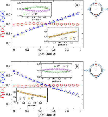
Figure 4: Comparison of the prediction of the perturbation theory and individual-based simulations at the level of the probabilities $P_{i}(x)=P_{i}^{+}(x)+P_{i}^{-}(x)$ to find a particle in state $i$ at position $x$ in the stationary state for the clock motifs shown in Fig. 3b,c. The insets indicate the splitting of these probabilities into up- and down-gradient motion, i.e. the probability densities $P_{i}^{\pm}$. Lines correspond to predictions of the perturbation theory, points show individual-based simulations. Parameters are identical to Fig. 3.

Concluding remarks

We studied the ability of active particles to perform taxis controlled by internal clocks. Our results reveal that clock designs with homogeneous transition rates $\gamma_{n}(x)$, i.e., $\gamma_{n}(x)=f[c(x)]$ for all $n$ with an arbitrary function $f[c]$, cannot generate a taxis response. It is important to realize that – despite the absence of a taxis response – the frequency of reversals may depend on the particle position, increasing or decreasing up-gradient depending on the clock design. We have shown that the clock has to fulfill the following requirements in order to generate a taxis response: (i) a number of ticks $M\geq 2$, (ii) at least one transition rate must depend on the external field, i.e., depends on $x$, and (iii) inhomogeneous transition rates, i.e., some or all transition rates should be pairwise distinct. Regarding the efficiency of the taxis response, we found that it increases with $M$, i.e. with the clock accuracy, though saturating for large values of $M$.

We stress that the obtained taxis responses are not due to the fact that we focused on velocity-reversing particles. All results hold true if we replace velocity reversals by tumbling events: if – instead of reversing with probability one – the particle reverses its direction of motion with probability $p$ and keeps it otherwise, all results reported here hold qualitatively true (cf. SM). By putting velocity reversals and tumbling events on an equal footing, it becomes evident that the crucial difference between the chemotactic mechanism of run-and-tumble bacteria, such as E. coli, and the one proposed here is the fundamentally distinct dynamics of the motility-control mechanisms, and not the type of turning maneuver (a tumble or a reversal) which is activated by the control mechanism. The two most compelling differences between these two mechanisms can be summarized as follows:

(a) In a uniform external field, i.e. in the absence of a gradient, run-and-tumble bacteria display an exponential distribution of run-times, and thus the temporal sequence of tumbling events is well-characterized by a single rate. In the here-proposed model, which is phenomenologically consistent with observations of run-and-reverse bacteria such as P. putida, the distribution of run-times is never exponential for $M>1$, but $\gamma$-shaped, cf. Fig. 1. This implies that the temporal sequence of reversals (or tumble events) cannot be parametrized by just a single rate, an observation indicating that the dynamics that controls the triggering of such events is more complex than a simple Poisson process Korobkova et al. (2006); Wang et al. (2017); we show that it may well be represented by a clock model.

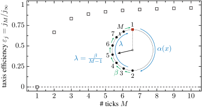
Figure 5: Taxis efficiency, characterized by the relative current $\varepsilon_{j}=j_{M}/j_{\infty}$, see text and Eq. (8), as a function of the number of ticks $M$, which measures the accuracy of the clock. The mean frequency $\lambda$ for the occurrence of the last $M\!-\!1$ ticks was fixed to be independent of $M$ by choosing $\beta=(M-1)\lambda$. The efficiency of sensing an external field increases with the accuracy of the clock. There is no chemotactic response for $M=1$. Parameters in arbitrary units (cf. Fig. 3): position of the current measurement $\bar{x}=0.5$, $\alpha(x)$ is a linear function with $\alpha(x)=0.75+0.5x$, $\lambda\!=\!1$, $v_{0}\!=\!0.01$, $L=1$.

(b) The canonical chemotaxis strategy of run-and-tumble bacteria relies on a memory: when experiencing a temporal increase in chemoattractant concentration, they decrease their tumble frequency. In the proposed clock-controlled taxis mechanism, in contrast to the classical chemotaxis picture, biased up-gradient motion can occur even when the tumbling frequency increases as the bacterium moves up-gradient. Moreover, depending on the clock design, we have observed (i) absence of taxis, (ii) up-gradient motion or (iii) down-gradient motion, even though the tumbling frequency was increasing with increasing concentration in all three cases, as illustrated in Fig. 3. This highlights the relevance of the clock architecture and indicates that the taxis direction is not dictated by the concentration dependency of the tumbling frequency, but rather by the clock design. In other words, we conclude from our results that it is generally not sufficient to measure the run-time bias only in order to infer the chemotaxis strategy of a microogranism but the measurement of the stationary concentration profile in a chemical gradient provides necessary, complementary information. We recall in this context that homogeneous clocks, where all transition rates are equal, imply a run-time bias at the single-particle level but will not yield a nonuniform concentration profile, i.e. particles will not accumulate at concentration maxima nor minima. Note also that the measurement of these profiles is experimentally managable, e.g. via microfluidic maze structures as reported recently Salek et al. (2019).

Altogether, the proposed clock-controlled taxis mechanism is a powerful conceptual toolbox that allows us to engineer a large variety of taxis responses, which may also play a key role in the design of simple robots Mijalkov et al. (2016) or for controlled assembly of active colloids Bäuerle et al. (2018); Karani et al. (2019). While the proposed phenomenological model is qualitatively consistent with experimental observations of P. putida, it is important to stress that we currently have no further mechanistic evidence that P. putida or other bacteria operate by such a clock. We insist on the phenomenological nature of the proposed clock model for sensing a signal, its internalization and processing, presumably involving cascades of biochemical events depicted by stochastic checkpoints. Identifying the intracellular mechanisms regulating the chemotactic responses of P. putida as well as other bacteria is a long-term experimental challenge beyond the scope of our current work. We thus hope that this study will open the door to a new series of experimental and theoretical works that advance our understanding of the directional navigation of bacteria.

See pages 1 of Supp_Inf.pdf

See pages 2 of Supp_Inf.pdf

See pages 3 of Supp_Inf.pdf

See pages 4 of Supp_Inf.pdf

See pages 5 of Supp_Inf.pdf

See pages 6 of Supp_Inf.pdf

See pages 7 of Supp_Inf.pdf