Massive Event-Shape Distributions at N²LL

Abstract

In a recent paper we have shown how to optimally compute the differential and cumulative cross sections for massive event-shapes at $\mathcal{O}(\alpha_{s})$ in full QCD. In the present article we complete our study by obtaining resummed expressions for non-recoil-sensitive observables to N²LL + $\mathcal{O}(\alpha_{s})$ precision. Our results can be used for thrust, heavy jet mass and C-parameter distributions in any massive scheme, and are easily generalized to angularities and other event shapes. We show that the so-called E- and P-schemes coincide in the collinear limit, and compute the missing pieces to achieve this level of accuracy: the P-scheme massive jet function in Soft-Collinear Effective Theory (SCET) and boosted Heavy Quark Effective Theory (bHQET). The resummed expression is subsequently matched into fixed-order QCD to extend its validity towards the tail and far-tail of the distribution. The computation of the jet function cannot be cast as the discontinuity of a forward-scattering matrix element, and involves phase space integrals in $d=4-2\varepsilon$ dimensions. We show how to analytically solve the renormalization group equation for the P-scheme SCET jet function, which is significantly more complicated than its 2-jettiness counterpart, and derive rapidly-convergent expansions in various kinematic regimes. Finally, we perform a numerical study to pin down when mass effects become more relevant.

1 Introduction

Since the late 70s, a class of observables called event shapes has been used to test and determine fundamental properties of QCD (for a review see  Dasgupta:2003iq ; Kluth:2006bw ), most notably to measure the strong coupling. As the name suggests, these observables contain information about the geometric momentum distribution of the final-state particle momenta. The (historic) main fields of application are $e^{+}e^{-}$ collisions and deep inelastic scattering (DIS), but today there also exist adaptations developed specifically for $pp$ colliders. In high-energy experiments most of the time it is sufficient to use the approximation that all particles in the final state are massless. If one is interested in high-precision calculations or in cases where the quark mass is a dominant effect, this approximation is no longer valid.

While the theoretical computation of event-shape distributions for massless quarks at $e^{+}e^{-}$ colliders has been pushed to unprecedented precision in recent years, including fixed-order results to $\mathcal{O}(\alpha_{s}^{3})$ GehrmannDeRidder:2007bj ; GehrmannDeRidder:2007hr ; Weinzierl:2008iv ; Ridder:2014wza ; Weinzierl:2009ms ; DelDuca:2016ily and resummation at next-to-next-to-leading-logarithm (N²LL) Hornig:2009vb ; Becher:2012qc ; Bell:2018gce and next-to-next-to-next-to-leading-logarithm (N³LL) Becher:2008cf ; Chien:2010kc ; Hoang:2014wka ; Moult:2018jzp ; HJM-theo , computations for massive quarks remain at a lower precision. Such high level of resummation for massless quarks has been achieved in most cases using Soft-Collinear Effective Theory (SCET) Bauer:2000ew ; Bauer:2000yr ; Bauer:2001ct ; Bauer:2001yt ; Bauer:2002nz (or in the equivalent formalism by Collins, Soper and Sterman Collins:1981uk ; Korchemsky:1998ev ; Korchemsky:1999kt ; Korchemsky:2000kp ; Berger:2003iw ), in which the most singular terms of the distribution are written in a factorized form, and summation of large logarithms is carried out with standard renormalization-group evolution. On the other hand, using the coherent branching formalism Catani:1992ua , the resummation can be automatized up to N²LL with numeric codes Banfi:2004yd ; Banfi:2014sua . The results have been extended to the case of oriented event shapes in Ref. Mateu:2013gya , and can be used to extract the strong coupling with high precision by comparing the theoretical expressions to LEP data, see e.g. Becher:2012qc ; Chien:2010kc ; Abbate:2010xh ; Abbate:2012jh ; Gehrmann:2012sc ; Hoang:2015hka ; HJM-fit .

A first step towards having a firmer theoretical control over massive event shapes was taken in Ref. Lepenik:2019jjk . In that article, the fixed-order differential and cumulative cross sections were computed at $\mathcal{O}(\alpha_{s})$ for any event shape. Since quark masses screen collinear divergences, there are only soft singularities that translate at threshold into two types of singular terms: a Dirac delta and a plus function (at higher orders other singular functions might appear). In Ref. Lepenik:2019jjk the coefficients of the delta and plus functions were computed analytically, providing a closed $1$-dimensional integral form for the former, and showing that the latter is universal. Furthermore, the delta function coefficient was provided in an analytic form for most event shapes. An algorithm was devised to compute the non-singular terms through a single integral (which can be carried out analytically in a few cases), a method much faster and accurate than binning the distribution in conjunction with a Monte Carlo integrator. In the present paper we complement those developments by adding resummation of large Sudakov logarithms at N²LL. This kind of resummation for boosted quarks has been worked out only for the hemisphere-mass (doubly differential) distribution in Refs. Fleming:2007qr ; Fleming:2007xt , which can be easily marginalized into heavy jet mass and 2-jettiness (and with extra little work, also into a variable called C-Jettiness in Ref. Lepenik:2019jjk ). In both cases, and only through recent computations that will be reviewed in the next paragraph, N³LL precision has been achieved. In this article we take the necessary steps to bring the accuracy to N²LL + $\mathcal{O}(\alpha_{s})$ for SCET-I type observables in the massive E- and P-schemes. These massive schemes were defined to better understand soft hadronization and affect the way in which the energy and momentum of each massive particle enters the computation of the event shape, while they have no effect on massless particles. In the P-scheme only three-momentum information is considered, whereas in the E-scheme the energy and particle direction are used.

Although SCET was first developed as an effective theory for massless particles, it was quickly generalized to include massive quarks in Ref. Leibovich:2003jd . Resummation is achieved in SCET by writing the most singular terms of the cross section as the product or convolution of various pieces: the hard matrix element, which is the squared modulus of the matching coefficient between SCET and QCD; the jet function, describing radiation collinear to the initiating partons; and the soft function, accounting for wide-angle soft radiation. Quark masses are infrared modes of the effective theory and therefore do not show up in the hard matching coefficient, but they do contribute to the jet (starting at one-loop) and soft (starting at two loops) functions. In the limit in which the difference between the jet and the heavy-quark massess is much smaller than either of those, a new physical scale emerges, requiring additional resummation of large logarithms. This is achieved by matching SCET onto boosted heavy-quark effective theory (bHQET). For jettiness all the ingredients necessary to build an N³LL-accurate cross section are known: bHQET jet function Jain:2008gb , SCET massive jet function Hoang:2019fze , and bHQET matching coefficient Hoang:2015vua , as well as the secondary production contributions Gritschacher:2013pha ; Pietrulewicz:2014qza (all up to two-loop level). The computations carried out in this article make possible N²LL resummation both in SCET and bHQET for other classes of event shapes. Masses can also modify the endpoint of the distribution, which is their only effect at LL and NLL. This threshold modification depends solely on the scheme used to define the massive event shape.

In the approach followed in Butenschoen:2016lpz to build the differential cross section, kinematic power corrections are taken into account in fixed-order perturbation theory by matching the SCET cross section onto full QCD. This setup was successfully applied to phenomenological analyses of massless event shapes, and is crucial to obtain reliable predictions in the tail and far-tail of the distribution. In the case of massive event shapes the situation is a bit more complex for two reasons: a) the partonic threshold is different in full QCD and the EFT, and b) the EFT prediction does not completely reproduce the singular terms at threshold. The reason is simple to understand: since the mass is an infrared mode, it is power-counted together with other infrared scales such as the quark virtuality, in such a way that power-suppressed terms include kinematic as well as mass corrections. Since the main focus of this article is on event shapes with mass-independent thresholds, issue a) is not relevant. At leading power, SCET and bHQET only predict the leading $\hat{m}$ behavior of the singular terms in QCD. It is however possible to modify the hard and jet functions to fully account for the singular terms in the factorization theorems, such that power corrections are not distributions and behave well close to threshold. We will show how to apply this prescription to event shapes in the E- and P-schemes.

Non-vanishing quark masses imply that the mass sensitivity can be tuned using different schemes for the event-shape definition. To the best of our knowledge, this possibility has only been studied in the context of fixed-order perturbation theory in Ref. Lepenik:2019jjk , and in the present work this analysis is continued by considering resummation of large logarithms. Furthermore, we complete the list of ingredients necessary for a full N²LL + $\mathcal{O}(\alpha_{s})$ computation, which are applied to the case study of P-scheme thrust, making our work a useful reference for upcoming studies. Our result is essential to consistently include bottom-quark mass effects in analyses that aim to extract $\alpha_{s}$ from fits to LEP data, and to clarify the top quark mass interpretation problem.

This article is organized as follows: in Sec. 2 we discuss kinematics in the dijet limit, which is the core for factorizing cross sections; in Sec. 3 we review the concept of massive schemes, explore how they affect the mass sensitivity of cross sections, and derive the implications they have for the SCET power counting; the factorization theorems in SCET and bHQET are presented in Sec. 4, in which also large-logarithm resummation is introduced; we carry out the computation of the SCET massive jet function in Sec. 5, and use this result in Sec. 6 to write down the fixed-order expression of the cross section in the dijet limit; in Sec. 7 we compute the bHQET jet function, and derive analytic results for the running of the non-distributional pieces of the SCET jet function in Sec. 8, presenting some useful expansions that can be implemented in different regions of the spectrum; kinematic, massive and non-perturbative power corrections are discussed in Sec. 9, while some numerical investigations are carried out in Sec. 10; finally, our conclusions are contained in Sec. 11. Some technical aspects of the computations are relegated to Appendices A and B.

2 Dijet Kinematics

In this section we study the kinematics of dijet events: two narrow, nearly back-to-back jets, plus additional soft radiation. In this situation the value of the event-shape is not far from its minimal value $e_{\min}$, and the SCET power-counting rules apply. Particles in such events can be either soft, $n$-collinear or $\bar{n}$-collinear, with momenta whose light-cone coordinates $p^{\mu}=(p^{+},p^{-},p^{\perp})$ scale like $p_{s}^{\mu}\sim Q(\lambda^{2},\lambda^{2},\lambda^{2})$, $p_{n}^{\mu}\sim Q(\lambda^{2},1,\lambda)$ and $p_{\bar{n}}^{\mu}\sim Q(1,\lambda^{2},\lambda)$ respectively, with $\lambda$ the SCET power-counting parameter. Since we are interested in the primary production of heavy quarks and $p^{2}=m^{2}$, for consistency one has that $\hat{m}\sim\lambda$ and soft particles are either massless or have $\hat{m}_{s}\lesssim\lambda^{2}$. The SCET scaling holds for momenta defined in the P- and E-schemes as well. In this limit it is possible to write the event-shape measurement $e$ as the sum of contributions from collinear (in both directions) and soft particles Bauer:2008dt ; Mateu:2012nk :

$$\overline{e}=e_{n}+e_{\bar{n}}+e_{s}\,,$$ (1)

where $\overline{e}$ denotes the event-shape measurement in the dijet limit at leading power, and we consider only soft perturbative particles. For SCET-I type observables, the three terms scale like $\lambda^{2}$ and are equally important. Moreover, $e_{n}$, $e_{\bar{n}}$ and $e_{s}$ can be written as a sum over single-particle contributions. If the event shape is already defined by a single sum of final-state particle momenta (as it is the case for thrust or angularities) this statement is trivial. When the event shape correlates momenta of final-state particles [ e.g. the definition involves a double sum (C-parameter) or there is a single sum squared (jet masses) ] the situation is more complicated. In the latter case one has to show explicitly that in this limit the leading contribution to the event shape can be written in the form of Eq. (1), as was done e.g. in Ref. Hoang:2014wka for C-parameter. Let us work out this decomposition for hemisphere masses, which are defined as the square of the total four-momentum flowing into one of the hemispheres, being those delimited by the plane normal to the thrust axis. Assuming the $z$ axis in the thrust direction, the mass of the plus hemisphere takes the following form in light-cone coordinates:

$$Q^{2}\rho_{+}=\sum_{i\in+}p_{i}^{+}\sum_{j\in+}p_{j}^{-}-\biggl{(}\sum_{i\in+}p^{\perp}_{i}\biggr{)}^{\!\!2}=\sum_{i\in+}p_{i}^{+}\sum_{j\in+}p_{j}^{-},$$ (2)

where we have used that the component of the total hemisphere momenta normal to the thrust axis is identically zero. Let us assume the negative direction of the $z$ axis pointing towards the plus hemisphere such that it does not contain $\bar{n}$-collinear particles (with $p_{z}>0$). In the dijet limit, particles $i$ and $j$ can be either soft or collinear, but if both are soft the corresponding contribution is $\rho^{s,s}\propto\mathcal{O}(\lambda^{4})$ and therefore power suppressed. Next we consider that $i$ is soft and $j$ is collinear, such that the leading contribution comes from the $p_{j}^{-}$ term:

$$Q^{2}\rho^{s}_{+}=\biggl{(}\sum_{j\in n}p_{j}^{-}\biggr{)}\!\biggl{(}\sum_{i\in s_{+}}p_{i}^{+}\biggr{)}=2\biggl{(}\sum_{j\in n}E_{j}\biggr{)}\!\biggl{(}\sum_{i\in s_{+}}p_{i}^{+}\biggr{)}=Q\!\sum_{i\in s_{+}}p_{i}^{+}=QP_{s_{+}}^{+},$$ (3)

where we have used that up to power corrections in the dijet limit $p_{i}^{-}=2E_{i}$ and the total available energy $Q$ is carried by collinear particles only and equally divided into each hemisphere, such that the total minus momentum flowing into the plus hemisphere is $Q$ up to power corrections. The set of soft particles that belong to the plus hemisphere is denoted by $s_{+}$. With an identical computation we get for the collinear-collinear contribution

$$Q\rho^{n}_{+}=\sum_{i\in c_{+}}p_{i}^{+}=P_{n}^{+}\,,$$ (4)

with $c_{+}$ the set of $n$-collinear particles. In the dijet limit we have $Q\rho_{+}=P_{s_{+}}^{+}+P_{n}^{+}$, which is equal to the total plus momentum entering the minus hemisphere. An identical reasoning leads to $Q\rho_{-}=P_{s_{-}}^{-}+P_{\bar{n}}^{-}$. Since we have not made any assumption on the mass of the particles, our result is valid for massless and massive quarks.

3 Massive Schemes

In this section we review the generalization of event-shape measurements for massive particles that go under the name of “massive schemes” (which should not be mistaken with the quantum field theory mass schemes such as pole, PS, 1S, MSR, $\overline{\mathrm{MS}}$, …). These schemes were introduced in an article by Salam and Wicke Salam:2001bd to study the effects of hadron masses on hadronization power corrections, which were further studied in Mateu:2012nk . Both studies consider light quarks only, such that massive schemes have no effect on partonic computations, but change the size of non-perturbative power corrections. For massive quarks, however, switching schemes can dramatically change the cross section, in particular its sensitivity to the quark mass, which is obviously of high interest either in cases where very accurate computations demand including quark mass corrections, or when they are the leading effect. A propaedeutic study of massive schemes for heavy quarks in event-shape cross sections was carried out in Ref. Lepenik:2019jjk , where fixed-order results were computed and subsequently analyzed. A more complete study demands resummation of large logarithms in the peak and tail of the distribution, and we aim to fill in this gap here.

Massless particles travel at the speed of light and their four-momenta satisfy $p^{2}=0$, which when translated into energy and momentum in a given frame implies $E_{p}=|\vec{p}\,|$. Therefore on can interchange $E_{p}\leftrightarrow|\vec{p}\,|$ in the event-shape definition with no visible effect. If particles become massive, $p^{2}=m^{2}$ and one has $E_{p}>|\vec{p}\,|$, meaning in turn that replacing the momentum magnitude by the energy (or vice versa) changes the value of the event shape. In this context, various massive schemes were defined to quantify this possibility, which reproduce the original “massless” definition in the limit $m\to 0$:

1. E-scheme: As indicated by its name, one replaces momenta by energies with the substitution $(p_{i}^{0},\vec{p}_{i})\to p_{i}^{0}\,(1,\vec{p}_{i}/|\vec{p}_{i}|)$. The scalar product takes the following form:

   $$p_{E}\!\cdot\!q_{E}=E_{p}E_{q}\biggl{(}1-\frac{\vec{p}\!\cdot\vec{q}}{|\vec{p}\,||\vec{q}\,|}\biggr{)}\,,$$ (5)

   such that $p_{E}^{2}=0$ even for massive particles. One advantage of this prescription is that hadronization corrections become universal. The variables called angularities Berger:2003pk were originally defined in this scheme.

2. P-scheme: Again the name suggests that energy gets replaced by momenta as $(p_{i}^{0},\vec{p}_{i})\to|\vec{p}_{i}|\,(1,\vec{p}_{i}/|\vec{p}_{i}|)$, and it happens that most of the classical event shapes were originally defined in this scheme: thrust Farhi:1977sg , C-parameter Parisi:1978eg ; Donoghue:1979vi and broadening Rakow:1981qn . The scalar product now reads $p_{P}\!\cdot\!q_{P}=|\vec{p}\,||\vec{q}\,|-\vec{p}\cdot\!\vec{q}$, which again implies $p_{P}^{2}=0$ for massless and massive particles.

3. M-scheme: The name “massive scheme” is used for event shapes that in their original definition were neither in the P- nor in the E-scheme, such as heavy jet mass Clavelli:1979md ; Chandramohan:1980ry ; Clavelli:1981yh . Their definition contains both energy and momentum and are the most sensitive to quark masses, in particular because in this scheme the usual relation $p^{2}=m^{2}$ is satisfied.

It is important to realize that four-momenta as defined in the E- and P-schemes are frame-dependent, and that event shapes are usually defined in terms of magnitudes measured in the center-of-mass frame. The usual light-cone decomposition applies in either scheme $S$

$$p_{S}\!\cdot\!q_{S}=\frac{1}{2}\,p_{S}^{+}q_{S}^{-}+\frac{1}{2}\,q_{S}^{+}p_{S}^{-}-\vec{p}_{S,\perp}\!\cdot\vec{q}_{S,\perp}\,,$$ (6)

with $S=E,P$. The specific definition of the event shapes just introduced can be found e.g. in the original papers and will not be repeated here unless necessary. They are also summarized, including a discussion on massive schemes, in Ref. Lepenik:2019jjk .

3.1 Mass Sensitivity

When studying the sensitivity of event shapes at parton level the leading order contribution for $e^{+}e^{-}$ annihilation comes from the production of a heavy quark-antiquark pair without additional radiation. In this case, the thrust axis is parallel to the three-momenta of the quarks, which makes trivial to calculate the threshold for two particles in the final state with equal mass $m$. Moreover, this simple computation sets the lower threshold even if additional gluons and (massless) quarks are radiated.

	$\tau$	$\tau_{a}$	$C$	$\rho$
M-scheme	$1-\beta$	$(1-\beta)^{\frac{2-a}{2}}(1+\beta)^{\frac{a}{2}}$	$12\hat{m}^{2}(1-\hat{m}^{2})$	$\hat{m}^{2}$
P- and E- schemes	$0$	$0$	$0$	$0$

Table 1: Threshold position for various event shapes in the case of primary production of a stable quark-antiquark pair in different massive schemes. We use $\beta=\sqrt{1-4\hat{m}^{2}}$, the velocity of the quarks at threshold in natural units.

The results in Tab. 1 show that for events in which a massive stable quark-antiquark pair is produced (primary production) only the M-scheme is sensitive to the quark mass while P- and E-schemes are not. In most of the events there will be some extra radiation present which will modify the former dijet into two fatter jets or an even more isotropic momentum distribution. For the observables we study, such processes will mainly contribute for event-shape values away from threshold adding subleading mass sensitivity (i.e. suppressed by a factor of $\alpha_{s}$) even in the P- and E-schemes, but will not substantially change the leading sensitivity of the M-scheme definition since it comes from the tree-level peak position. From this we can conclude that the M-scheme is preferred if the aim is a mass-sensitive observable (e.g. for quark mass determinations), but in case that one seeks a mass-insensitive observable, the P- and E-schemes are a better choice.

3.2 Massive Schemes in the Collinear Limit

Collinear particles in the $n$ direction satisfy $E_{p}=(p^{+}+p^{-})/2=p^{-}/2+\mathcal{O}(\lambda^{2})$ and also $|\vec{p}\,|=\sqrt{E_{p}^{2}-m^{2}}=p^{-}/2+\mathcal{O}(\lambda^{2})$ such that the E-scheme ($Q=\sum_{i}E_{i}$) and P-scheme ($Q_{p}\equiv\sum_{i}|\vec{p}_{i}|$) normalizations are the same at leading power. Let us compute the four-momenta of massive $n$-collinear particles in the E- and P-schemes. Since we have seen that $E_{p}/|\vec{p}\,|=1+\mathcal{O}(\lambda^{2})$, the “large” (or label) components $p^{-}$ and $p^{\perp}$ are the same in any scheme. Let us then focus in the small $p^{+}$ momenta, which in the massive scheme takes the following form (for $n$-collinear particles the $z$ component of momenta is negative):

$$p^{+}=E_{p}+p_{z}=E_{p}-\sqrt{|\vec{p}\,|^{2}-|\vec{p}_{\perp}|^{2}}=E_{p}-\sqrt{E^{2}_{p}-E_{\perp}^{2}}\simeq\frac{E_{\perp}^{2}}{2E_{p}}+\mathcal{O}(\lambda^{4})\,,$$ (7)

where we have used the so-called perpendicular energy $E_{\perp}\equiv\sqrt{|\vec{p}_{\perp}|^{2}+m^{2}}$. The computation of $p^{+}$ in the P-scheme is very similar since one only has to use $|\vec{p}\,|$ instead of $E_{p}$

$$p_{P}^{+}=|\vec{p}\,|+p_{z}=|\vec{p}\,|-\sqrt{|\vec{p}\,|^{2}-|\vec{p}_{\perp}|^{2}}\simeq\frac{|\vec{p}_{\perp}|^{2}}{2E_{p}}+\mathcal{O}(\lambda^{4})=p^{+}-\frac{m^{2}}{p^{-}}+\mathcal{O}(\lambda^{4})\,,$$ (8)

where we notice that in the second step $p_{P}^{+}$ takes the same analytic form as in Eq. (7) with the replacements $E_{p}\to|\vec{p}\,|$ and $E_{\perp}\to|\vec{p}_{\perp}|$, in the third step we use $|\vec{p}\,|=E_{p}+\mathcal{O}(\lambda^{2})$, and in the last step we replace $|\vec{p}_{\perp}|^{2}=p^{+}p^{-}-m^{2}$ and $E_{p}=p^{-}/2+\mathcal{O}(\lambda^{2})$. It is important to notice that in general $p_{P}^{+}\neq p^{+}$ because $m^{2}/(p^{+}p^{-})\simeq\mathcal{O}(1)$. Moreover, the mass that appears in Eq. (8) (and in any other event-shape measurement function) comes from kinematic on-shell considerations and therefore corresponds to the pole scheme. Finally, let us compute the E-scheme $p^{+}$ component, and for that we only need to make the replacement $p_{z}\to p_{z}E_{p}/|\vec{p}\,|$ in Eq. (7):

$$p_{E}^{+}=E_{p}+\frac{E_{p}}{|\vec{p}\,|}\,p_{z}=\frac{E_{p}}{|\vec{p}\,|}\,p_{P}^{+}=p_{P}^{+}+\mathcal{O}(\lambda^{4})\,,$$ (9)

where in the last step we again have used $E_{p}/|\vec{p}\,|=1+\mathcal{O}(\lambda^{2})$. Since for collinear particles (in any direction) $p_{P}^{\mu}=p_{E}^{\mu}$ at leading power, we can safely conclude that at this order the collinear measurements for all event shapes take the same form in the P- and E-schemes, but is in general different from the M-scheme. In what follows we will work out the collinear measurement for a few event shapes.

Thrust

The original thrust definition is already in the P-scheme and reads

$$\tau^{P}=\frac{1}{Q_{P}}\min_{\hat{t}}\sum_{i}(|\vec{p}_{i}|-|\hat{t}\cdot\vec{p}_{i}|)\,,$$ (10)

with $\hat{t}$ the thrust axis. For $n$-collinear particles one has $|\hat{t}\cdot\vec{p}_{i}|=-p_{z}$ and therefore up to power corrections we have

$$Q\tau^{P}_{c}=Q\tau^{E}_{c}=\sum_{i\in+}p_{P,i}^{+}=\sum_{i\in+}\biggl{(}p_{i}^{+}-\frac{m_{i}^{2}}{p_{i}^{-}}\biggr{)}\,,$$ (11)

where we already indicate that the collinear measurement is the same in the E-scheme. In Ref. Stewart:2009yx an M-scheme generalization of thrust, dubbed 2-jettiness, was introduced

$$\tau^{J}=\frac{1}{Q}\min_{\hat{t}}\sum_{i}(E_{i}-|\hat{t}\cdot\vec{p}_{i}|)\,,$$ (12)

such that its collinear limit is the total plus momentum flowing into the plus hemisphere $Q\tau^{J}_{c}=\sum_{i\in+}p_{i}^{+}$. Since the measurement is completely inclusive, the computation of the jet function can be carried out as the imaginary part of a forward-scattering matrix element. This is not the case for the E- and P-schemes if quark masses are non-vanishing.

Hemisphere Jet Masses

We already worked out the collinear measurement for heavy jet mass in Eq. (4), and getting the P-scheme measurement is equally simple since Eq. (2) still applies with minimal modifications:

$$Q^{2}\rho_{+}^{P}=\biggl{(}\sum_{i\in+}|\vec{p}_{i}|\biggr{)}^{\!\!2}-\biggl{(}\sum_{i\in+}p^{z}_{i}\biggr{)}^{\!\!2}=\biggl{[}\,\sum_{i\in+}(|\vec{p}_{i}|+p^{z}_{i})\biggr{]}\!\biggl{[}\,\sum_{j\in+}(|\vec{p}_{j}|-p^{z}_{j})\biggr{]}=\sum_{i\in+}p_{P,i}^{+}\sum_{j\in+}p_{P,j}^{-}\,,$$ (13)

where we again use that the total perpendicular momentum vanishes and use the identity $a^{2}-b^{2}=(a+b)(a-b)$. With this result we can trivially obtain the collinear measurement using that $p_{P,j}^{-}=2E_{j}+\mathcal{O}(\lambda^{2})$:

$$Q\rho_{c,+}^{P}=Q\rho_{c,+}^{E}=\sum_{i\in+}\biggl{(}p_{i}^{+}-\frac{m_{i}^{2}}{p_{i}^{-}}\biggr{)}\,,$$ (14)

that matches the P-scheme thrust result. The total perpendicular momentum does not vanish in the E-scheme, since there is not such thing as E-scheme three-momentum conservation (in the same way, P-scheme energy is not conserved either). However, in the dijet limit the perpendicular components are already $\mathcal{O}(\lambda)$ and therefore $p^{\perp}_{E}=p^{\perp}+\mathcal{O}(\lambda^{3})$, making $\sum_{i\in+}p^{\perp}_{E,i}\propto\mathcal{O}(\lambda^{3})$, thence power suppressed, such that the result in Eq. (14) is also valid for the E-scheme.

C-parameter

In Ref. Hoang:2014wka it was shown how the C-parameter measurement splits into the sum of soft and collinear contributions in the dijet limit. The proof relied on the particles being massless, so it cannot be taken for granted that it will work when quarks have a non-zero mass. Here we carry out a similar proof valid for massive particles as well. C-parameter is defined already in the P-scheme as

$$C^{P}= \,\frac{3}{2Q_{P}^{2}}\sum_{i,j}|\vec{p}_{i}||\vec{p}_{j}|\sin^{2}(\theta_{ij})=\frac{3}{2Q_{P}^{2}}\sum_{i,j}|\vec{p}_{i}||\vec{p}_{j}|[1+\cos(\theta_{ij})][1-\cos(\theta_{ij})]$$ (15)

$$= \,\frac{3}{2Q_{P}^{2}}\sum_{i,j}\frac{(|\vec{p}_{i}||\vec{p}_{j}|+\vec{p}_{i}\!\cdot\!\vec{p}_{j})(|\vec{p}_{i}||\vec{p}_{j}|-\vec{p}_{i}\!\cdot\!\vec{p}_{j})}{|\vec{p}_{i}||\vec{p}_{j}|}\,,$$

where we simply use $\sin^{2}(\theta_{ij})=1-\cos^{2}(\theta_{ij})=[1+\cos(\theta_{ij})][1-\cos(\theta_{ij})]$ and the definition of the euclidean scalar product to get to the final form. Next one can express the result in terms of P-scheme light-cone coordinates using Eq. (6) as follows

$$C^{P}= \,\frac{3}{2Q_{P}^{2}}\sum_{i,j}\frac{(2|\vec{p}_{i}||\vec{p}_{j}|-p_{P,i}\!\cdot\!p_{P,j})\,p_{P,i}\!\cdot\!p_{P,j}}{|\vec{p}_{i}||\vec{p}_{j}|}$$ (16)

$$= \,\frac{3}{2Q_{P}^{2}}\sum_{i,j}\frac{(p_{P,i}^{+}\,p_{P,j}^{+}+p_{P,i}^{-}\,p_{P,j}^{-}+2\vec{p}_{\perp,i}\!\cdot\vec{p}_{\perp,j})(p_{P,i}^{+}\,p_{P,j}^{-}+p_{P,i}^{-}\,p_{P,j}^{+}-2\vec{p}_{\perp,i}\!\cdot\vec{p}_{\perp,j})}{(p_{P,i}^{+}+p_{P,i}^{-})(p_{P,j}^{+}+p_{P,j}^{-})}\,,$$

with a similar result in the E-scheme. Arguments analogous to those used in Ref. Hoang:2014wka apply, and we focus on the collinear measurement only. First consider that both $i$ and $j$ are $n$-collinear such that the SCET scaling implies

$$C^{P}_{nn}=\frac{3}{Q^{2}}\biggl{[}\biggl{(}\sum_{i\in n}p^{+}_{P,i}\biggr{)}\!\biggl{(}\sum_{j\in n}p^{-}_{P,j}\biggr{)}\!-\biggl{(}\sum_{i\in n}\vec{p}_{\perp,i}\biggr{)}\!\cdot\!\biggl{(}\sum_{j\in n}\vec{p}_{\perp,j}\biggr{)}\!\biggr{]}=\frac{3}{Q}\sum_{i\in n}p^{+}_{P,i}+\mathcal{O}(\lambda^{3})\,,$$ (17)

where once again we use that the total collinear perpendicular momenta flowing into the plus hemisphere is zero up to power corrections. One gets an analogous result for $C^{P}_{\bar{n}\bar{n}}$, while if $i$ is $n$-collinear and $j$ is $\bar{n}$-collinear we get (we already include a factor of $2$ to account for the case in which $i$ is $\bar{n}$-collinear and $j$ is $n$-collinear)

$$C^{P}_{n\bar{n}}\,=\, \frac{3}{Q^{2}}\biggl{[}\!\biggl{(}\sum_{i\in n}p^{+}_{P,i}\biggr{)}\!\biggl{(}\sum_{j\in\bar{n}}p^{+}_{P,i}\biggr{)}\!+\!\biggl{(}\sum_{i\in n}p^{-}_{P,i}\biggr{)}\!\biggl{(}\sum_{j\in\bar{n}}p^{-}_{P,i}\biggr{)}\!+2\biggl{(}\sum_{i\in n}\vec{p}_{\perp,i}\biggr{)}\!\cdot\!\biggl{(}\sum_{j\in\bar{n}}\vec{p}_{\perp,j}\biggr{)}\!\biggr{]}$$

$$\,=\, \frac{3}{Q}\biggl{(}\sum_{i\in n}p^{+}_{P,i}+\sum_{i\in\bar{n}}p^{-}_{P,i}\biggr{)}\!+\mathcal{O}(\lambda^{3})\,.$$ (18)

Summing up the contributions in Eqs. (17) and (3.2) we obtain the collinear measurement in the P- and E-schemes:

$$QC^{P}_{c}=QC^{E}_{c}=6\sum_{i\in+}p_{P,i}^{+}=6\sum_{i\in+}\biggl{(}p_{i}^{+}-\frac{m_{i}^{2}}{p_{i}^{-}}\biggr{)}\,,$$ (19)

identical to that of thrust or the hemisphere masses up to a factor of $6$. The computation for the E-scheme is identical, relies on arguments already exposed, and therefore will not be repeated. For the M-scheme C-jettiness variable introduced in Ref. Gardi:2003iv it was shown in Ref. Preisser:mthesis that the collinear measurement takes the simple form $QC^{J}_{c}=6\sum_{i\in+}p_{i}^{+}$. Therefore, for the reduced C-parameter variable $\widetilde{C}\equiv C/6$ the collinear measurement for the three event shapes we consider coincide in every massive scheme.

4 Factorization Theorems

For simplicity we consider the well-known case of thrust (in either massive scheme), which can be easily modified to obtain the corresponding factorized results for C-parameter (changing the soft function and taking into account factors of $6$ in the measurement function) or heavy jet mass (using the hemisphere jet and soft functions, and including two convolutions, one per hemisphere). After having shown that in the three schemes considered Eq. (1) holds, the derivation of the factorization theorem is obtained following the steps outlined in Ref. Bauer:2008dt . The leading hadronization corrections (which are soft) can also be factorized as an extra convolution with the so-called shape function, and even though they are included in our numerical analysis, for the sake of conciseness we ignore them in this section. Likewise, we include kinematic and mass power corrections in our final analysis, but postpone their discussion until Sec. 9

4.1 SCET

The value of the quark mass can have different hierarchies with respect to the (EFT) hard, jet, and soft scales. These are the natural scales of the various matrix elements appearing in the factorization theorem shown in Eq. (20), that is, the scales that produce no large logarithms. They can be identified with physical scales: $\mu_{H}$ is similar to the center-of-mass energy $Q$, $\mu_{J}$ can be associated to the perpendicular momentum of a jet with respect to its axis, and $\mu_{S}$ is of the order of the soft-particles’ energies. In Refs. Gritschacher:2013pha ; Pietrulewicz:2014qza it was extensively discussed how to setup a consistent variable-flavor number scheme for final-state jets accounting for primarily and secondarily produced massive quarks. Four scenarios can be defined for the cases in which $m>\mu_{H}$ (scenario I, which is of no interest for primary quarks since there is no energy to produce them), $\mu_{H}>m>\mu_{J}$ (scenario II, relevant for very boosted heavy quarks, and better described in bHQET), $\mu_{J}>m>\mu_{S}$ (scenario III) and $m<\mu_{S}$ (scenario IV). Each of them has a different factorization theorem and renormalization group evolution setup. Even though the heavy quark mass is a fixed parameter, the jet and soft scales depend on the event-shape value and therefore they change along the spectrum, such that several scenarios might occur in a given distribution. For simplicity, we assume the quark mass is always smaller than the soft scale, such that we stay in scenario IV even in the peak of the distribution. In this way, we avoid having to deal with integrating out the heavy quark mass and the partonic factorization formula reads

$$\frac{1}{\sigma_{0}}\frac{\text{d}\hat{\sigma}_{\rm SCET}}{\text{d}\tau}=Q^{2}H(Q,\mu)\!\!\int_{0}^{Q(\tau-\tau_{\rm min})}\!\!\text{d}\ell\,J_{\tau}(Q^{2}\tau-Q\ell,\mu)S_{\tau}(\ell,\mu)\,,$$ (20)

with $\sigma_{0}$ the Born or point-like (massless) cross section, $H$ and $S_{\tau}$ the hard and soft functions, respectively, and

$$J_{\tau}(s,\mu)\equiv\!\int_{s_{\rm min}}^{s-s_{\rm min}}\!\text{d}s^{\prime}J_{n}(s-s^{\prime},\mu)J_{n}(s^{\prime},\mu)\,,$$ (21)

the thrust jet function, which is the convolution of two single-hemisphere jet functions. The M-scheme hemisphere jet function has support for $s>s_{\rm min}=m^{2}$, what sets the integration limits in Eq. (21). Accordingly, the thrust jet function has support for $s>2s_{\min}$, implying that the minimal value for 2-jettiness is $\tau^{J}_{\rm min}=2\hat{m}^{2}$. We shall present the computation of the M- and P-scheme SCET jet function in Sec. 5. The definition of the soft function in terms of Wilson lines can be found e.g. in Ref. Bauer:2008dt and the corresponding expression for the jet function will be given in Sec. 5. The factorization formula takes a simpler form in Fourier space

$$\frac{1}{\sigma_{0}}\frac{\text{d}\hat{\sigma}_{\rm SCET}}{\text{d}\tau}=\frac{Q}{2\pi}H(Q,\mu)\!\!\int\!\text{d}x\,e^{ixp}\tilde{J}_{\tau}\!\biggl{(}\frac{x}{Q},\mu\biggr{)}\tilde{S}_{\tau}(x,\mu)\,,$$ (22)

with $p=Q(\tau-\tau_{\rm min})$ and $\tilde{J}_{\tau}$ and $\tilde{S}$ the Fourier transforms of the jet and soft functions, respectively. The thrust jet function in position space is the square of its hemisphere counterpart, and can be computed as follows

$$\tilde{J}_{\tau}(y,\mu)=\!\int_{0}^{\infty}\!\!\text{d}\bar{s}\,e^{-i\bar{s}y}J_{\tau}(\bar{s}+s_{\min},\mu)=\tilde{J}_{n}(y,\mu)^{2}\,.$$ (23)

In Eqs. (20) and (22) all matrix elements are evaluated at the same renormalization scale $\mu$. In order to minimize large logarithms that appear in each of them one should use RGE equations to evaluate them at their respective natural scales, denoted by $\mu_{H}\sim Q$, $\mu_{J}\sim Q\sqrt{\tau}$ and $\mu_{S}\sim Q\tau$, such that for small $\tau$ there is a strict hierarchy among those: $\mu_{H}>\mu_{J}>\mu_{S}$ and the SCET scaling parameter takes the value $\lambda\sim\sqrt{\tau}$. The form and solution of the renormalization group equations is also simpler in position space. Using those and changing variables to $y=x/p$ one arrives at

$$\frac{1}{\sigma_{0}}\frac{\text{d}\hat{\sigma}_{\rm SCET}}{\text{d}\tau}=\frac{H(Q,\mu_{H})}{p}\biggl{(}\frac{e^{\gamma_{E}}\mu_{S}}{p}\biggr{)}^{\!\!\tilde{\omega}}R(Q,\mu_{i})\!\int\!\frac{\text{d}y}{2\pi}\,e^{iy}(i\,y)^{\tilde{\omega}}\tilde{J}_{\tau}\!\biggl{(}\frac{y}{Qp},\mu_{J}\biggr{)}\tilde{S}_{\tau}\!\biggl{(}\frac{y}{p},\mu_{S}\biggr{)}\,,$$ (24)

where $\mu_{i}$ denotes collectively all renormalization scales (including the common $\mu$) and we use the following compact notation

$$R(Q,\mu_{i})=\, Q\biggl{(}\frac{\mu_{H}}{Q}\biggr{)}^{\!\!-2\tilde{\omega}_{H}}e^{\tilde{k}}\biggl{(}\frac{\mu^{2}_{J}}{Q\mu_{S}}\biggr{)}^{\!\!\tilde{\omega}_{J}}\,,$$

$$\tilde{k}=\, \tilde{k}_{H}+\tilde{k}_{J}+\tilde{k}_{S}\,, \tilde{\omega} =\tilde{\omega}_{J}-2\tilde{\omega}_{S}\,,$$

$$\tilde{\omega}_{S}=\, \tilde{\omega}_{\Gamma_{c}}(\mu_{S},\mu), \tilde{\omega}_{J} =\tilde{\omega}_{\Gamma_{c}}(\mu_{J},\mu),$$ (25)

$$\tilde{\omega}_{H}=\, \tilde{\omega}_{\Gamma_{c}}(\mu_{H},\mu)\,, \tilde{k}_{S} =\tilde{\omega}_{\gamma_{S}}(\mu_{S},\mu)-2\tilde{k}_{\Gamma_{c}}(\mu_{S},\mu)\,,$$

$$\tilde{k}_{H}=\, \tilde{\omega}_{\gamma_{H}}(\mu_{H},\mu)-2\tilde{k}_{\Gamma_{c}}(\mu_{H},\mu)\,, \tilde{k}_{J} =\tilde{\omega}_{J}(\mu_{J},\mu)+4\tilde{k}_{\Gamma_{c}}(\mu_{J},\mu)\,,$$

with $\tilde{\omega}$ and $\tilde{k}$ the exponential running kernels defined in terms of integrals over the SCET and QCD anomalous dimensions as follows

$$\tilde{\omega}_{\gamma}(\mu_{0},\mu)=\, 2\!\int^{\alpha_{\mu}}_{\alpha_{0}}\!\text{d}\alpha\,\frac{\gamma(\alpha)}{\beta_{\rm QCD}(\alpha)}\,,$$ (26)

$$\tilde{k}_{\gamma}(\mu_{0},\mu)=\, 2\!\int^{\alpha_{\mu}}_{\alpha_{0}}\!\text{d}\alpha\,\frac{\gamma(\alpha)}{\beta_{\rm QCD}(\alpha)}\int^{\alpha}_{\alpha_{0}}\text{d}\alpha^{\prime}\frac{1}{\beta_{\rm QCD}(\alpha^{\prime})}\,.$$

Here $\gamma$ can refer to cusp or non-cusp anomalous dimensions, and their dependence on $\alpha$ is in the form of perturbative series that define their respective coefficients

$$\!\!\!\beta_{\rm QCD}(\alpha)=-2\,\alpha_{s}\!\sum_{n=1}\beta_{n-1}\Bigl{(}\frac{\alpha}{4\pi}\Bigr{)}^{\!\!n},\quad\Gamma_{\rm cusp}(\alpha)=\!\sum_{n=1}\Gamma_{n}\Bigl{(}\frac{\alpha}{4\pi}\Bigr{)}^{\!\!n},\quad\gamma(\alpha)=\!\sum_{n=1}\gamma_{n}\Bigl{(}\frac{\alpha}{4\pi}\Bigr{)}^{\!\!n}.$$ (27)

The integrals in Eq. (26) can be solved analytically in terms of the anomalous-dimension coefficients if an expansion in $\alpha_{s}$ is carried out. Their explicit form up to N³LL can be found e.g. in Ref. Abbate:2010xh . General expressions valid for arbitrarily high order can also be derived and will be given elsewhere.

The jet function of a massive quark contains terms which are distributions, and hence easy to Fourier transform, plus others which are regular functions, and to the best of our knowledge it seems impossible to find an analytic expression in position space for them. Up to one loop, the momentum-space hemisphere jet function can be decomposed in the following form:

$$J_{n}(\bar{s}+s_{\rm min},\mu)=\, \delta(\bar{s})+\frac{\alpha_{s}(\mu)}{4\pi}C_{F}\Bigl{[}J_{\rm dist}(\bar{s},\mu)+\frac{1}{m^{2}}J_{\rm nd}\Bigl{(}\frac{\bar{s}}{m^{2}}\Bigr{)}\Bigr{]}+\mathcal{O}(\alpha_{s}^{2})\,,$$ (28)

$$J_{\rm dist}(\bar{s},\mu)=\, \frac{1}{\mu^{2}}J_{m=0}\Bigl{(}\frac{\bar{s}}{\mu^{2}}\Bigr{)}+\frac{1}{m^{2}}J_{m}\Bigl{(}\frac{\bar{s}}{m^{2}}\Bigr{)}\,,$$

where the massive corrections, either with distributions $J_{m}$ or fully non-distributional $J_{\rm nd}$, are $\mu$-independent dimensionless functions with support for positive values of their (dimensionless) arguments. The $\mu$ dependence of $J_{\rm dist}$ is entirely determined from the jet and QCD anomalous dimensions, does not depend on the quark mass, and therefore can be fully accounted for in the massless jet function of Eq. (28). The only piece that needs an explicit computation in the E- and P-schemes is $J_{\rm nd}$, since the rest can be obtained using consistency conditions and results obtained in Refs. Lepenik:2019jjk and Fleming:2007xt .

The integral in Eq. (24) can be easily solved for all terms involving only distributions, and generic formulas can be found for instance in Ref. Becher:2008cf . For the non-distributional piece of the jet function we carry out resummation in momentum space, and at one loop it is multiplied by the hard and soft functions at tree-level only. Therefore, using Eq. (23) in (24) and carrying out the $y$ integration, the non-distributional part of the 1-loop partonic cross section reads

$$\frac{1}{\sigma_{0}}\frac{\text{d}\hat{\sigma}_{\rm nd}}{\text{d}\tau}=\, \frac{C_{F}\alpha_{s}(\mu_{J})}{2\pi}\frac{R(Q,\mu_{i})}{\hat{m}^{2}\Gamma(-\tilde{\omega})}(Qe^{\gamma_{E}}\mu_{S})^{\tilde{\omega}}\!\int_{2s_{\rm min}}^{Q^{2}\tau}\!\!\text{d}s\,J_{\rm nd}\Bigl{(}\frac{s-2s_{\rm min}}{m^{2}}\Bigr{)}(Q^{2}\tau-s)^{-1-\tilde{\omega}}$$

$$=\, \frac{C_{F}\alpha_{s}(\mu_{J})}{2\pi}\frac{R(Q,\mu_{i})}{\hat{m}^{2}}\biggl{[}\frac{\mu_{S}e^{\gamma_{E}}}{Q(\tau-\tau_{\rm min})}\biggr{]}^{\!\tilde{\omega}}I_{\rm nd}\Bigl{(}\tilde{\omega},\frac{\tau-\tau_{\rm min}}{\hat{m}^{2}}\Bigr{)}\,,$$ (29)

$$I_{\rm nd}(\tilde{\omega},y)=\, \frac{y^{\tilde{\omega}}}{\Gamma(-\tilde{\omega})}\int_{0}^{y}\text{d}x\,(y-x)^{-1-\tilde{\omega}}J_{\rm nd}(x)=\frac{1}{\Gamma(-\tilde{\omega})}\int_{0}^{1}\text{d}z\,(1-z)^{-1-\tilde{\omega}}J_{\rm nd}(zy)\,.$$

The lower limit of integration in the first line has been moved to $2s_{\rm min}$ since below that value the jet function has no support. In the E- and P-schemes $s_{\min}=0$ so we have not lost any generality. To get to the second line we have switched variables in the integral to $s=xm^{2}+2s_{\rm min}$, and to obtain the second expression for $I_{\rm nd}(\tilde{\omega},y)$ we switch variables to $x=zy$. For the partonic cumulative distribution one gets instead

$$\!\hat{\Sigma}_{\rm nd}(\tau_{c})\, \equiv\frac{1}{\sigma_{0}}\!\int_{0}^{\tau_{c}}\!\!{\rm d}\tau\,\frac{\text{d}\sigma_{\rm nd}}{\text{d}\tau}$$ (30)

$$=\frac{C_{F}\alpha_{s}(\mu_{J})}{2\pi}\frac{R(Q,\mu_{i})}{\hat{m}^{2}}\frac{\mu_{S}e^{\gamma_{E}}}{Q}\!\biggl{[}\frac{\mu_{S}e^{\gamma_{E}}}{Q(\tau_{c}-\tau_{\rm min})}\biggr{]}^{\tilde{\omega}-1}I_{\rm nd}\Bigl{(}\tilde{\omega}-1,\frac{\tau_{c}-\tau_{\rm min}}{\hat{m}^{2}}\Bigr{)}.$$

To make the function $I(\tilde{\omega},y)$ smooth in the no resummation limit, achieved when $\tilde{\omega}\to 0$, one can integrate by parts to obtain

$$I_{\rm nd}(\tilde{\omega},y)=\frac{1}{\Gamma(1-\tilde{\omega})}\biggl{[}\,y\!\!\int_{0}^{1}{\rm d}z(1-z)^{-\tilde{\omega}}J_{\rm nd}^{\prime}(zy)+J_{\rm nd}(0)\biggr{]}\,,$$ (31)

with $J_{\rm nd}^{\prime}$ the derivative of the $J_{\rm nd}$ function. This form is particularly useful if the integration has to be carried out numerically, making it more convergent and defining its analytic continuation to values $0<\tilde{\omega}<1$. Further integration by parts can be implemented to define the integral for even larger values of $\tilde{\omega}$. If a closed analytical form is found, this procedure is unnecessary.

Although the discussion in this section has been carried out assuming the pole mass for the heavy quark, it is straightforward to convert the result to a short-distance scheme. In the scenarios in which SCET applies, the $\overline{\mathrm{MS}}$ scheme is perfectly adequate. In scenario II it is more convenient to employ low-scale short-distance schemes such as the MSR mass Hoang:2008yj ; Hoang:2017suc .

4.2 bHQET

If the heavy quark mass is large enough or if the jet is very narrow one enters scenario II, in which the jet and heavy quark masses are close to each other, corresponding to very boosted quarks. In this kinematic situation, a new physical scale emerges $\mu_{B}\sim Q\tau/{\hat{m}}\sim\mu_{S}/{\hat{m}}$, such that there is a new hierarchy between scales: $\mu_{H}>m>\mu_{B}>\mu_{S}$. A practical way to see how this becomes manifest is looking at the structure of the one-loop jet function in Eq. (28). Since the non-distributional terms are power suppressed when $s\to s_{\rm min}$, it is enough to focus on the terms with distributions, which generically read

$$\frac{1}{\mu^{2}}J_{m=0}\Bigl{(}\frac{\bar{s}}{\mu^{2}}\Bigr{)}=\, A\,\delta(\bar{s})+\frac{B}{\mu^{2}}\biggl{[}\frac{\mu^{2}}{\bar{s}}\biggr{]}_{+}+\frac{C}{\mu^{2}}\biggl{[}\frac{\mu^{2}\log(\bar{s}/\mu^{2})}{\bar{s}}\biggr{]}_{+}\,,$$ (32)

$$\frac{1}{m^{2}}J_{m}\Bigl{(}\frac{\bar{s}}{m^{2}}\Bigr{)}=\, A_{m}\,\delta(\bar{s})+\frac{B_{m}}{m^{2}}\biggl{[}\frac{m^{2}}{\bar{s}}\biggr{]}_{+}+\frac{C_{m}}{m^{2}}\biggl{[}\frac{m^{2}\log(\bar{s}/m^{2})}{\bar{s}}\biggr{]}_{+}\,,$$

where the coefficients $A,\,B$ and $C$ (with or without subindex $m$) depend neither on $\mu$ nor on $m$. In scenarios III and IV one has $\bar{s}\lesssim m^{2}$ and therefore the choice $\mu^{2}\sim\bar{s}$ makes sure there are no large logarithms in neither term (the massless limit is smooth since $J_{m}+J_{\rm nd}\to 0$ when $m\to 0$ and no new class of large logarithms emerges). On the other hand, if $\bar{s}\ll m^{2}$ the choice $\mu^{2}\sim\bar{s}$ cannot prevent the logarithms in $J_{m}$ from becoming large.

The massive shell of the heavy quark carrying momentum $p=mv+k$ with $v^{2}=1$ gets integrated out as a dynamical degree of freedom giving raise to heavy-quark effective theory Eichten:1989zv ; Isgur:1989vq ; Isgur:1989ed ; Georgi:1990um . The remaining degrees of freedom are referred to as ultracollinear and carry residual momentum $k$. In the heavy quark rest frame [ in which $v^{\mu}=(1,1,\vec{0}_{\perp})$ ] they are soft $k^{\mu}=\Delta(1,1,1)$, with $\Delta\ll m$ a low-energy scale, being able to interact with each other and with color sources representing the integrated-out heavy quarks. In the center-of-mass frame these momenta get boosted and a hierarchy is generated among their light-cone components

$$v_{+}^{\mu}=\, \biggl{(}\frac{m}{Q},\frac{Q}{m},\vec{0}_{\perp}\!\biggr{)}\,, k_{+}^{\mu} \sim\Delta\biggl{(}\frac{m}{Q},\frac{Q}{m},1\!\biggr{)}\,, q_{s}^{\mu} =\frac{m\Delta}{Q}(1,1,1)\,,$$ (33)

$$v_{-}^{\mu}=\, \biggl{(}\frac{Q}{m},\frac{m}{Q},\vec{0}_{\perp}\!\biggr{)}\,, k_{-}^{\mu} \sim\Delta\biggl{(}\frac{Q}{m},\frac{m}{Q},1\!\biggr{)}\,,$$

where we have included momenta $q_{s}$ which is soft in the center-of-mass frame. The two boosted copies of HQET are matched onto SCET in order to account for global soft radiation, such that the heavy quark and ultracollinear particles can interact with soft degrees of freedom. The typical off-shellness of ultracollinear particles is softer than for collinear degrees of freedom which are part of SCET.

Using this framework, it is possible to derive a factorization theorem for the partonic cross section Fleming:2007qr which effectively separates physics at the different involved scales.

$$\!\!\!\frac{1}{\sigma_{0}}\frac{\text{d}\hat{\sigma}_{\rm bHQET}}{\text{d}\tau}\!=\!Q^{2}H(Q,\mu_{m})H_{m}\!\biggl{(}\!m,\frac{Q}{m},\mu_{m},\mu\!\biggr{)}\!\!\!\int\!\!\text{d}\ell\,B_{\tau}\!\biggl{(}\!\frac{Q^{2}(\tau-\tau_{\rm min})-Q\ell}{m},\mu\!\biggr{)}\!S_{\tau}(\ell,\mu),$$ (34)

where the hard and soft functions are the same as in the SCET factorization theorem, but there is an additional matching coefficient $H_{m}$ between SCET and bHQET. The jet function $B_{\tau}(\hat{s})$ is different from $J_{\tau}$ in SCET, has support for $\hat{s}>0$, its mass dependence is only through a global $1/m$ factor and contains only distributions. It is also the convolution of two hemisphere bHQET jet functions $B_{n}$:

$$B_{\tau}(\hat{s},\mu)=m\!\int_{0}^{\hat{s}}\!\text{d}\hat{s}^{\prime}B_{n}(\hat{s}-\hat{s}^{\prime},\mu)B_{n}(\hat{s}^{\prime},\mu)\,,$$ (35)

whose operator definition shall be given in Sec. 7. Since $H$ and $H_{m}$ are the same for all event shapes and $S_{\tau}$ does not depend on the quark mass (it sees only light degrees of freedom), the anomalous dimension of the $B_{n}$ function is the same in any massive scheme. In turn this implies that all terms in the jet function except for the Dirac delta are fixed by consistency and hence are the same in the M-, P- and E-schemes. Knowing $H$, $H_{m}$ and $S_{\tau}$ at one loop, the delta function coefficient in $B_{n}$ can be obtained taking the $\hat{m}\to 0$ limit of the result quoted in Ref. Lepenik:2019jjk for the full QCD prediction of the threshold delta function coefficient. In this sense, our computation in Sec. 7 will be just a sanity check. The $H_{m}$ matching coefficient and bHQET jet function satisfy $J_{\tau}(s+s_{\rm min})=H_{m}B_{\tau}(s/m)[1+\mathcal{O}(s/m^{2})]$, such that both factorization theorems smoothly join. For the various arguments exposed in this paragraph, this also implies that the coefficients $B_{m}$ and $C_{m}$ in Eq. (32) do not depend on the massive scheme, and they are known from the 2-jettiness computation of Ref. Fleming:2007xt . Therefore, different massive schemes can differ only in $A_{m}$ and the $J_{\rm nd}$, but knowing the one-loop hard and soft functions, $A_{m}$ can be obtained again from the massless limit of the full-QCD threshold result.

Carrying out resummation in bHQET is identical to massless SCET. Since we will limit our numerical analysis to situations in which it is sufficient to use SCET with masses, we will not give further details on how to solve the corresponding RGE equations, which can be found elsewhere. Moreover, we will not provide a detailed discussion on how to switch to a short-distance mass scheme in this setup.

5 SCET Jet Function Computation

The jet function accounts for the dynamics of collinear particles within the hemisphere. Since the collinear measurement function in the P- and E-schemes is not the total plus momentum, it cannot be computed as the discontinuity of a forward-scattering amplitude, as was done in Fleming:2007qr ; Fleming:2007xt . Instead, one has to use the definition given in Ref. Bauer:2008dt , which after a small modification to match the form of our factorization theorem and minimal manipulations can be cast into the form:

$$J_{n}(s,\mu) =\!\int\!\frac{{\rm d}\ell^{+}\!}{2\pi}\,\mathcal{J}_{n}(s,\ell^{+})\,,$$ (36)

$$\mathcal{J}_{n}(s,\ell^{+}) =\frac{1}{4N_{c}}{\rm Tr}\!\!\int\!{\rm d}^{d}x\,e^{i\ell x}\left\langle 0\right|\not{{\overline{n}}}\chi_{n}(x)\,\delta(s-Q^{2}\hat{e}_{n})\,\overline{\chi}_{n,Q}(0)\!\left|0\right\rangle\,,$$

with $\chi_{n,Q}$ the jet field with total minus momentum equal to $Q$, $d=4-2\varepsilon$ the space-time dimension in dimensional regularization, $\ell^{-}=Q$ and $\vec{\ell}_{\perp}=\vec{0}$ due to label momentum conservation, and the trace is taken over spin and color indices. The $n$-collinear event-shape operator $\hat{e}_{n}$ acting on some final state $\left|X\right\rangle$ pulls out $e_{n}(X)$, the contribution from $n$-collinear particles to the value of the event shape: $\hat{e}_{n}\left|X\right\rangle=e_{n}(X)\left|X\right\rangle$. To simplify the expression in the second line of Eq. (36) we insert the identity $I=\sum_{X}\left|X\right\rangle\!\left\langle X\right|$ after the delta function and shift the field $\chi_{n,Q}(x)$ to $x=0$ employing the momentum operator. Using the label operators for the large components of the momenta, the sum over $X$ can be carried out and we obtain the following convenient expression:

$$J_{n}(s,\mu)=\frac{(2\pi)^{d-1}}{N_{C}}\mathrm{Tr}\biggl{[}\frac{\overline{n}\!\!\!/}{2}\langle 0|\chi_{n}(0)\delta(s-Q\hat{e}_{n})\delta^{(d-2)}(\vec{\mathcal{P}}_{X}^{\perp})\delta(\mathcal{\bar{P}}-Q)\bar{\chi}_{n}(0)|0\rangle\biggr{]}\,.$$ (37)

For practical computations one inserts a complete set of states after $\delta(\mathcal{\bar{P}}-Q)$

$$\sum_{X}\left|X\right\rangle\!\left\langle X\right|\equiv\sum_{n=1}\,\sum_{\rm spin}\,\int\prod_{i=1}^{n}\frac{{\rm d}^{d-1}\vec{p}_{i}}{(2\pi)^{d-1}(2E_{i})}|X_{n}\rangle\langle X_{n}|\,,$$ (38)

where we exclude the vacuum from the sum because it does not contribute to the jet function. Each term in the sum over $n$ can include several contributions, accounting for various particle species (heavy or light quarks and gluons), and the sum over polarizations affects all particles in the final state. The perturbative expansion of the jet function in powers of $\alpha_{s}$ is obtained by adding more particles to the sum as well as more virtual (loop) contributions to the matrix elements that appear after inserting the identity, which in compact form can be written as

$$J_{n}(s,\mu)=\frac{(2\pi)^{d-1}}{N_{C}}\sum_{X}\delta^{(d-2)}(\vec{p}_{X}^{\perp})\delta(p_{X}^{-}-Q)\delta[s-Q^{2}e_{n}(X)]{\rm Tr}\!\biggl{[}\gamma^{0}\frac{\overline{n}\!\!\!/}{2}\left|\left\langle\>0|\chi_{n}(0)|X\>\right\rangle\right|^{2}\biggr{]}\,.$$ (39)

For the computation of the P-scheme hemisphere jet function one does not need any regularization beyond taking the space-time dimension from $4$ to $d=4-2\varepsilon$. In the following we carry out the computation of the jet function using Eq. (37) for both 2-jettiness and P-scheme thrust. Although the result is already known for the former, it is instructive to repeat its computation to highlight the differences between the two approaches. In a way, the computation that uses Eq. (37) can be obtained applying Cutkosky rules to directly obtain the imaginary part of the forward-scattering matrix element.

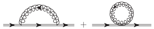
Figure 1: One-loop diagrams contributing to the wave-function renormalization at $\mathcal{O}(\alpha_{s})$.

It is important to remember that $\chi_{n}$ in Eq. (37) is composed of bare SCET (quark and gluon) fields, and that it is convenient to carry out our computations using perturbation theory “around” those (that is, we will not use the so-called renormalized perturbation theory). For the jettiness computation through the discontinuity of the forward matrix element, this entails that the wave-function renormalization factor

$$Z_{\xi}=1+\frac{\alpha_{s}C_{F}}{4\pi}\Biggl{[}-\frac{3}{\varepsilon}+6\log\!{\biggl{(}\frac{m}{\mu}\biggr{)}}-4\Biggr{]}+\mathcal{O}(\alpha_{s}^{2})\,,$$ (40)

computed with the diagrams shown in Fig. 1 (the soft-gluon contribution vanishes), never appears directly. The mass in Eq. (40) should be understood as the pole scheme. When using Eq. (37) one needs to account for $Z_{\xi}^{1/2}$ since this factor is precisely the overlap between the quantum (bare) collinear field $\xi_{n}$ and the physical collinear state $\left|q_{n}\right\rangle$: $\left\langle 0\right|\xi_{n}\left|q_{n}(\vec{p},s)\right\rangle=Z_{\xi}^{1/2}u_{s}(\vec{p}\,)$, with $u$ a particle spinor in the collinear limit, and $s$, $\vec{p}$ the spin and $3$-momentum of the on-shell collinear quark. On the other hand, when using Eq. (37) self-energy diagrams on external legs are not included, since their effect is already accounted for in the $Z_{\xi}^{1/2}$ factor, and it is in this way that one has a one-to-one correspondence with the computation through the imaginary part of the forward matrix element.

The computation at leading order is simple enough that can be carried out for the two massive schemes simultaneously. The corresponding tree-level diagram is shown in Fig. 2, where the double line represents a heavy quark and the dashed line marks which particles are on-shell. To compute the phase-space integration it is convenient to use the following parametrization

$$\frac{{\rm d}^{d-1}\vec{p}}{2E_{p}}=\, \frac{{\rm d}p^{-}}{2p^{-}}\,\theta(p^{-})\,{\rm d}^{d-2}\vec{p}_{\perp}\,,$$ (41)

$$\int\!{\rm d}^{d-2}\vec{p}_{\perp}=\, \frac{2\pi^{1-\varepsilon}}{\Gamma(1-\varepsilon)}|\vec{p}_{\perp}|^{1-2\varepsilon}\!\!\int\!{\rm d}|\vec{p}_{\perp}|\,,$$

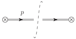
Figure 2: Lowest order diagram for the jet function.

which implies that $p^{+}$ has to be expressed in terms of the minus and perpendicular components through the on-shell condition $p^{+}=(m^{2}+|\vec{p}_{\perp}|^{2})/p^{-}$, and since the mass appears through on-shell kinematic relations it corresponds always to the pole scheme. In the second line we have carried out the angular integrals for the perpendicular momentum, assuming that matrix elements depend only on its magnitude. We then obtain

$$J_{n}^{\rm tree}(s)\!=\!\!\int\!\frac{{\rm d}p^{-}}{2p^{-}}{\rm d}^{d-2}\vec{p}_{\perp}\delta^{(d-2)}(\vec{p}_{\perp})\delta(p^{-}-Q)\delta[s-Q^{2}e_{n\!}(X)]\sum_{s}{\rm Tr}\!\biggl{[}\frac{\overline{n}\!\!\!/}{2}u_{s}(p)\overline{u}_{s}(p)\biggr{]}\!=\delta(s-s_{\min}),$$ (42)

where we have used that the trace of the polarization sum equals $2p^{-}$ and have integrated all delta functions except the one with the measurement. The color trace cancels the $1/N_{c}$ prefactor, and the on-shell condition implies $p^{+}=m^{2}/Q$, such that for the $2$-particle collinear measurement we get

$$e_{J}(X)=\frac{p^{+}}{Q}=\frac{m^{2}}{Q^{2}}\,,\qquad e_{\tau}(X)=\frac{p^{+}}{Q}-\frac{m^{2}}{p^{-}}=0\,,$$ (43)

which correspond to $e_{\rm min}$. To include the wave-function renormalization at $\mathcal{O}(\alpha_{s})$ one only needs to multiply this result by $Z_{\xi}$.

5.1 Virtual Radiation

The contribution from virtual gluons can be carried out for the two massive schemes simultaneously since the phase-space integration is identical to the tree-level computation. There are two diagrams contributing, as shown in Fig. 3, which yield the same result, so we will compute only one of them which will be multiplied by a factor of $2$. Pulling out a collinear gluon field from the Wilson line and using the Feynman rules for massive collinear quarks we obtain the following integral for the leftmost diagram:

$$J_{1}^{\rm virt}=-2iC_{F}g_{s}^{2}\tilde{\mu}^{2\varepsilon}\!\!\!\int\!\!\frac{{\rm d}^{d}\ell}{(2\pi)^{d}}\frac{\bar{n}(p+\ell)}{(\bar{n}\ell)\ell^{2}[(p+\ell)^{2}-m^{2}]}\equiv-2iC_{F}g_{s}^{2}(I_{1}+p^{-}I_{2})\,,$$ (44)

where $\tilde{\mu}^{2}=\mu^{2}e^{\gamma_{E}}/(4\pi)$, the factor of $2$ comes from the product $\bar{n}n$ and the Casimir $C_{F}$ from the color trace with two Gell-Mann matrices. We are left with two master integrals $I_{1}$ and $I_{2}$ that can be solved using Feynman parameters for the former

$$\!\!\!I_{1}=\!\!\int_{0}^{1}\!\!{\rm d}x\!\!\int\!\!\frac{{\rm d}^{d}\ell}{(2\pi)^{d}}\frac{\tilde{\mu}^{2\varepsilon}}{(\ell^{2}-x^{2}m^{2})^{2}}=\!\frac{i\,\Gamma(\varepsilon)e^{\varepsilon\gamma_{E}}}{4\pi}\!\!\int_{0}^{1}\!\!{\rm d}x\biggl{(}\frac{xm}{\mu}\biggr{)}^{\!\!-2\varepsilon}\!\!\!=\!\frac{i}{(4\pi)^{2}}\frac{\Gamma(\varepsilon)e^{\varepsilon\gamma_{E}}}{(1-2\varepsilon)}\biggl{(}\frac{m}{\mu}\biggr{)}^{\!\!-2\varepsilon}\!\!.$$ (45)

and with a combination of Feynman and Georgi parameters for the latter

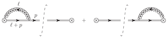
Figure 3: Virtual diagrams contributing to the jet function at $\mathcal{O}(\alpha_{s})$.

$$I_{2}=\, 2\!\!\int_{0}^{\infty}\!\!{\rm d}\lambda\!\!\int_{0}^{1}\!\!{\rm d}x\!\!\int\!\!\frac{{\rm d}^{d}\ell}{(2\pi)^{d}}\frac{(1-x)\tilde{\mu}^{2\varepsilon}}{[\ell^{2}-x^{2}m^{2}-x(1-x)\lambda]^{3}}$$

$$=\, \!-\!\frac{i\,\mu^{2\varepsilon}e^{\gamma_{E}}}{(4\pi)^{2}}\,\Gamma(1+\varepsilon)\!\!\int_{0}^{1}\!\!{\rm d}x\,x^{-1-\varepsilon}\!\!\int_{0}^{\infty}\!\!{\rm d}\lambda\biggl{\{}x(1-x)p^{-}\!\biggl{[}\lambda+\frac{m^{2}x}{(1-x)p^{-}}\biggr{]}\biggr{\}}^{\!-1-\varepsilon}$$ (46)

$$=\, \!-\!\frac{i}{(4\pi)^{2}}\frac{\Gamma(\varepsilon)e^{\gamma_{E}}}{p^{-}}\biggl{(}\frac{m}{\mu}\biggr{)}^{\!\!-2\varepsilon}\!\!\!\int_{0}^{1}\!\!{\rm d}x\,x^{-1-2\varepsilon}=\frac{i}{(4\pi)^{2}}\frac{\Gamma(\varepsilon)}{2\varepsilon p^{-}}\biggl{(}\frac{m}{\mu}\biggr{)}^{\!\!-2\varepsilon}\,.$$

Adding those two results we find a closed expression for $J_{1}^{\rm virt}$:

$$J_{1}^{\rm virt}=\, \frac{\alpha_{s}C_{F}}{4\pi}\frac{e^{\varepsilon\gamma_{E}}\Gamma(1+\varepsilon)}{\varepsilon^{2}(1-2\varepsilon)}\biggl{(}\frac{m}{\mu}\biggr{)}^{\!\!-2\varepsilon}$$ (47)

$$=\, \frac{\alpha_{s}C_{F}}{4\pi}\biggl{\{}\frac{1}{\varepsilon^{2}}+\frac{2}{\varepsilon}\biggl{[}1-\log\biggl{(}\frac{m}{\mu}\biggr{)}\biggr{]}+4+\frac{\pi^{2}}{12}-4\log\biggl{(}\frac{m}{\mu}\biggr{)}+2\log^{2}\biggl{(}\frac{m}{\mu}\biggr{)}\biggr{\}}\,.$$

Interestingly, this result is zero in the massless limit (which has to be taken before expanding in $\varepsilon$). Therefore, using dimensional regularization, only real-radiation diagrams contribute. The $m$ appearing in Eq. (47) is strictly speaking bare, but since we limit our computation to $\mathcal{O}(\alpha_{s})$ we can safely take it as the pole mass, as the difference between these two is a higher order correction. Implementing this result to the jet function computation and integrating the real momentum results in adding a factor of $\delta(e_{n}-e_{\min})$. Multiplying by $2$, expanding in $\varepsilon$ and adding the wave-function renormalization, which is obviously a virtual contribution, we obtain

$$J_{n}^{\rm virt}(s,\mu)=\frac{\alpha_{s}C_{F}}{4\pi}\,\delta(s-s_{\min})\!\biggl{[}\frac{2}{\varepsilon^{2}}+\frac{1}{\varepsilon}-\frac{4}{\varepsilon}\log\Bigl{(}\frac{m}{\mu}\Bigr{)}+4+\frac{\pi^{2}}{6}-2\log\Bigl{(}\frac{m}{\mu}\Bigr{)}+4\log^{2}\Bigl{(}\frac{m}{\mu}\Bigr{)}\!\biggr{]},$$ (48)

which is the final result of this section. Equation (48) should be valid also for SCET-II type observables since the 1-particle phase space is not yet afflicted by rapidity divergences.

5.2 Real Radiation

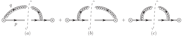
Figure 4: Real-radiation diagrams contributing to the jet function at $\mathcal{O}(\alpha_{s})$.

Since the phase-space integrals with two particles do not fully collapse with the Dirac delta functions, the real radiation contributions differ depending on the collinear measurement. The diagrams that contribute at $\mathcal{O}(\alpha_{s})$ are shown in Fig. 4, where we have omitted the term in which both gluons are radiated from the Wilson line since it vanishes. Diagrams (a) and (b) give identical contributions and therefore we will compute one of them which will be multiplied by a factor of $2$. For all the real contributions label-momentum conservation implies $\vec{q}_{\perp}=-\vec{p}_{\perp}$ and $q^{-}=Q-p^{-}$, which together with the Heaviside function in Eq. (41) sets the integration limits for $p^{-}$ between $0$ and $Q$. For the first diagram, after integrating the gluon momenta with the delta functions and carrying out the angular perpendicular integration one gets

$$J_{a}^{\rm real}(s,\mu)=\frac{4\alpha_{s}C_{F}\,Q\tilde{\mu}^{2\varepsilon}}{(4\pi)^{1-\varepsilon}\Gamma(1-\varepsilon)}\!\!\int_{0}^{Q}\!{\rm d}p^{-}\frac{p^{-}}{Q-p^{-}}\frac{|\vec{p}_{\perp}|^{1-2\varepsilon}{\rm d}|\vec{p}_{\perp}|}{m^{2}(Q-p^{-})^{2}+Q^{2}|\vec{p}_{\perp}|^{2}}\,\delta(s-Q^{2}e_{n})\,.$$ (49)

Since this diagram involves gluons radiated from Wilson lines, one expects $1/\varepsilon^{2}$ poles, implying also harder integrals. On the other hand, since the corresponding Feynman rule is simpler, the result is also shorter. For the third (symmetric) diagram, which does not need a factor of two, the result reads

$$J_{c}^{\rm real}(s,\mu)=\, \frac{\alpha_{s}C_{F}\,Q^{2}e^{\varepsilon\gamma_{E}}\mu^{2\varepsilon}}{(2\pi)\Gamma(1-\varepsilon)}\!\!\int_{0}^{Q}\!{\rm d}p^{-}\delta(s-Q^{2}e_{n})\,\frac{(Q-p^{-})(p^{-})^{2}|\vec{p}_{\perp}|^{1-2\varepsilon}{\rm d}|\vec{p}_{\perp}|}{m^{2}(Q-p^{-})^{2}+Q^{2}|\vec{p}_{\perp}|^{2}}$$ (50)

$$\times\biggl{[}\frac{2(1-\varepsilon)(|\vec{p}_{\perp}|^{2}+m^{2})}{(p^{-})^{2}}-2(1-\varepsilon)\frac{m^{2}}{Q^{2}}+\frac{4(2-\varepsilon)m^{2}}{Qp^{-}}\biggr{]}.$$

Since Feynman rules are more cumbersome for gluons radiated from a massive quark, the result is lengthier. On the other hand, since these correspond to boosted QCD processes single $1/\varepsilon$ poles are expected to appear, meaning that no special treatment for the integral is necessary.

5.2.1 P-scheme Thrust

To solve the integrals in the previous section, the thrust measurement must be expressed in terms of $p^{-}$ and $|\vec{p}_{\perp}|$. Since the gluon is massless and the quark has mass $m$ we have

$$Q^{2}\tau=Q\biggl{(}p^{+}+q^{+}-\frac{m^{2}}{p^{-}}\biggr{)}=Q\,|\vec{p}_{\perp}|^{2}\biggl{(}\frac{1}{p^{-}}+\frac{1}{Q-p^{-}}\biggr{)}=\frac{Q^{2}|\vec{p}_{\perp}|^{2}}{(Q-p^{-})p^{-}}\,,$$ (51)

which is mass independent. With this result we can use the measurement delta function to integrate $|\vec{p}_{\perp}|$

$$\delta(s-Q^{2}\tau)=\frac{(Q-p^{-})p^{-}}{2|\vec{p}_{\perp}|Q^{2}}\,\delta\biggl{(}\!|\vec{p}_{\perp}|-\frac{\sqrt{(Q-p^{-})s\,p^{-}}}{Q}\,\biggr{)}\,.$$ (52)

Switching variables to $p^{-}=Qx$ we find the following 1-dimensional integral for $J_{a}$:

$$J_{a,P}^{\rm real}(s,\mu)=\, \frac{C_{F}\alpha_{s}\,e^{\varepsilon\gamma_{E}}}{2\pi m^{2}\Gamma(1-\varepsilon)}\biggl{(}\frac{s}{\mu^{2}}\biggr{)}^{\!\!-\varepsilon}\!\!\!\!\int_{0}^{1}\!{\rm d}x\,\frac{x^{2-\varepsilon}(1-x)^{-1-\varepsilon}}{1-x\bigl{(}1-\frac{s}{m^{2}}\bigr{)}}\,.$$ (53)

The complication arises because the integral diverges as $1/\varepsilon^{2}$ and contains distributions. The divergence comes from the $(1-x)^{-1-\varepsilon}$ factor, but the subtraction around $x=1$ behaves as $1/s$, which combined with the $s^{-\varepsilon}$ prefactor implies a new divergence and invalidates the subtraction. This pathological behavior is usual in two-loop computations involving double integrals, and the standard way of solving it is using sector decomposition Binoth:2000ps . To do so, one needs to get rid of distributions by considering the cumulative jet function, which converts Eq. (53) into a double integral. In Appendix A we show how to use this general method to solve the integral, and follow in this section an easier, albeit less general, procedure. Before that, we solve the integral for the massless case, which is not affected by the problem just described, and is valid for 2-jettiness and thrust:

$$J_{a,m=0}^{\rm real}(s,\mu)=\, \!-\!\frac{C_{F}\alpha_{s}e^{\gamma_{E}}}{(2\pi)\mu^{2}}\biggl{(}\frac{s}{\mu^{2}}\biggr{)}^{\!\!-1-\varepsilon}\frac{\Gamma(2-\varepsilon)}{\varepsilon\Gamma(2-2\varepsilon)}$$ (54)

$$=\, \frac{C_{F}\alpha_{s}}{(2\pi)}\!\Biggl{[}\!\biggl{(}\frac{1}{\varepsilon^{2}}+\frac{1}{\varepsilon}+2-\frac{\pi^{2}}{4}\biggr{)}\delta(s)-\frac{1}{\mu^{2}}\!\biggl{(}\frac{\mu^{2}}{s}\biggr{)}_{\!\!+}\!\biggl{(}\frac{1}{\varepsilon}+1\biggr{)}\!+\!\frac{1}{\mu^{2}}\!\biggl{(}\frac{\mu^{2}\log(s/\mu^{2})}{s}\biggr{)}_{\!\!+}\,\Biggr{]}.$$

In the second line we have expanded the result around $\varepsilon=0$ to obtain distributions using the identity

$$x^{-1+\varepsilon}=\frac{1}{\varepsilon}\delta(x)+\sum_{n=0}\frac{\varepsilon^{n}}{n!}\biggl{[}\frac{\log^{n}(x)}{x}\biggr{]}_{+}.$$ (55)

For the $m>0$ case we can transform the integral using hypergeometric function identities. Since these special functions will appear also in Sec. (8), we remind here its integral definition (the hypergeometric function is symmetric with respect to its first two arguments):

$$_{2}F_{1}(a,b,c,z)=\, \frac{\Gamma(c)}{\Gamma(b)\Gamma(c-b)}\!\int_{0}^{1}\!\text{d}x\,x^{b-1}(1-x)^{c-b-1}(1-zx)^{-a}\,$$ (56)

$$=\, (1-z)^{c-b-a}{}_{2}F_{1}(c-a,c-b,c,z)\,,$$

where the second line is the so called Euler transformation. The integral in Eq. (53) is already in this canonical form and therefore we can write

$$J_{a,P}^{\rm real}(s,\mu)= -\!\frac{\Gamma(3-\varepsilon)\,C_{F}\alpha_{s}}{(2\pi)m^{2}\varepsilon\Gamma(3-2\varepsilon)}\biggl{(}\frac{s}{\mu^{2}}\biggr{)}^{\!\!-\varepsilon}{}_{2}F_{1}\!\biggl{(}1,3-\varepsilon,3-2\varepsilon,1-\frac{s}{m^{2}}\biggr{)}$$ (58)

$$= -\!\frac{\Gamma(3-\varepsilon)\,C_{F}\alpha_{s}}{(2\pi)m^{2}\varepsilon\Gamma(3-2\varepsilon)}\biggl{(}\frac{s}{m^{2}}\biggr{)}^{\!\!-1-2\varepsilon}\!\!\biggr{(}\frac{\mu^{2}}{m^{2}}\biggl{)}^{\!\!\varepsilon}{}_{2}F_{1}\!\biggl{(}2-2\varepsilon,-\varepsilon,3-2\varepsilon,1-\frac{s}{m^{2}}\biggr{)}$$

$$=\, \frac{C_{F}\alpha_{s}}{(2\pi)m^{2}\Gamma(1-\varepsilon)}\biggl{(}\frac{s}{m^{2}}\biggr{)}^{\!\!-1-2\varepsilon}\!\!\biggr{(}\frac{\mu^{2}}{m^{2}}\biggl{)}^{\!\!\varepsilon}\!\int_{0}^{1}\!\!{\rm d}x(1-x)^{2-\varepsilon}x^{-1-\varepsilon}\!\biggl{[}1-x\!\biggl{(}1-\frac{s}{m^{2}}\biggr{)}\!\biggr{]}^{-2+2\varepsilon}\!,$$

where in the second step we have used Euler’s identity and in the third we write the hypergeometric function back as an integral. The integration in the last term can be easily expanded in $\varepsilon$ using Eq. (55), and defining $\tilde{s}\equiv s/m^{2}$ we have 

$$I_{3}(\tilde{s})\equiv\int_{0}^{1}\!{\rm d}x\,(1-x)^{2-\varepsilon}x^{-1-\varepsilon}[1-x(1-\tilde{s})]^{-2+2\varepsilon}=-\frac{1}{\varepsilon}-\tilde{s}\!\!\int_{0}^{1}\!{\rm d}x\,\frac{[2-(2-\tilde{s})x]}{[1-(1-\tilde{s})x]^{2}}$$ (59)

$$+\varepsilon\!\!\int_{0}^{1}\!{\rm d}x\frac{2(1-x)^{2}\log[1-x(1-\tilde{s})]+\tilde{s}x[2-(2-\tilde{s})x+2]\log(x)-(1-x)^{2}\log(1-x)}{x[1-(1-\tilde{s})x]^{2}}$$

$$=-\frac{1}{\varepsilon}+\frac{\tilde{s}\,[1-\tilde{s}+\!(2-\tilde{s})\log(\tilde{s})]}{(1-\tilde{s})^{2}}+\varepsilon f_{1}(\tilde{s})\equiv-\frac{1}{\varepsilon}+\tilde{s}\,f_{0}(\tilde{s})+\varepsilon f_{1}(\tilde{s})+\mathcal{O}(\varepsilon^{2})\,,$$

with $f_{1}(s)$ a function involving a dilogarithm. This result can be reexpanded in $\varepsilon$ together with the prefactor ${\tilde{s}}^{\,-1-2\varepsilon}$, responsible for the appearance of distributions, finding then

$${\tilde{s}}^{\,-1-2\varepsilon}I_{3}(\tilde{s})=\frac{2}{\varepsilon^{2}}\,\delta(\hat{s})-\frac{1}{\varepsilon}\biggl{(}\frac{1}{\hat{s}}\biggr{)}_{\!\!+}+2\biggl{(}\frac{\log(\hat{s})}{\hat{s}}\biggr{)}_{\!\!+}-\frac{1}{2}f_{1}(0)\,\delta(\hat{s})+f_{0}(\hat{s})+\mathcal{O}(\varepsilon)\,.$$ (60)

Therefore one only needs $f_{1}(0)$, which takes a simple form

$$f(0)=\!\int_{0}^{1}\!{\rm d}x\,\frac{\log(1-x)}{x}=-\frac{\pi^{2}}{6}\,.$$ (61)

Putting all partial results together and expanding in $\varepsilon$ we get the following expression

$$J_{a,P}^{\rm real}(s,\mu)=\, \frac{C_{F}\alpha_{s}}{2\pi}\biggl{\{}\delta(s)\biggl{[}\frac{1}{2\varepsilon^{2}}+\frac{1}{\varepsilon}\log\Bigl{(}\frac{m}{\mu}\Bigr{)}+\log^{2}\Bigl{(}\frac{m}{\mu}\Bigr{)}+\frac{\pi^{2}}{24}\biggr{]}+\frac{2}{\mu^{2}}\biggl{[}\frac{\mu^{2}\log(s/\mu^{2})}{s}\biggr{]}_{\!+}$$

$$\!-\!\biggl{[}\frac{1}{\varepsilon}+2\log\Bigl{(}\frac{m}{\mu}\Bigr{)}\biggr{]}\frac{1}{\mu^{2}}\biggl{(}\frac{\mu^{2}}{s}\biggr{)}_{\!\!+}-\frac{1}{s-m^{2}}-\frac{s-2m^{2}}{(s-m^{2})^{2}}\log\biggl{(}\frac{s}{m^{2}}\biggr{)}\biggr{\}}.$$ (62)

The result is divergent for $s\to m^{2}$, although at that kinematic point there is no physical phenomenon that implies a singularity. We therefore expect that the singularity will cancel when adding together all real-radiation diagrams.

For the cut self-energy diagram in Fig. 4 (c), performing the same change of variable as in Eq. (53) we arrive at

$$J_{c,P}^{\rm real}(s,\mu)= \,\frac{C_{F}\alpha_{s}\,e^{\varepsilon\gamma_{E}}}{(2\pi)\Gamma(1-\varepsilon)}\biggl{(}\frac{s}{\mu^{2}}\biggr{)}^{\!\!-\varepsilon}$$ (63)

$$\times\!\int_{0}^{1}\!{\rm d}x\,\frac{x^{-\varepsilon}(1-x)^{1-\varepsilon}}{[s(1-x)+xm^{2}]^{2}}\{(1-\varepsilon)(1-x)xs-m^{2}[2(1-x)-(1-\varepsilon)x^{2}]\}\,.$$

To see how the $1/\varepsilon$ divergence occurs, we compute first the massless limit of $J_{c}^{\rm real}$, for which we get

$$J_{c,m=0}^{\rm real}(s,\mu)= \,\frac{C_{F}\alpha_{s}\,(1-\varepsilon)\,e^{\varepsilon\gamma_{E}}}{(2\pi)\mu^{2}\Gamma(1-\varepsilon)}\biggl{(}\frac{s}{\mu^{2}}\biggr{)}^{\!\!-1-\varepsilon}\!\!\!\!\int_{0}^{1}\!{\rm d}x\,x^{1-\varepsilon}(1-x)^{-\varepsilon}$$ (64)

$$= \,\frac{C_{F}\alpha_{s}\,e^{\varepsilon\gamma_{E}}\Gamma(2-\varepsilon)}{(4\pi)\mu^{2}\Gamma(2-2\varepsilon)}\biggl{(}\frac{s}{\mu^{2}}\biggr{)}^{\!\!-1-\varepsilon}=\frac{C_{F}\alpha_{s}}{4\pi}\biggl{[}\frac{1}{\mu^{2}}\biggl{(}\frac{\mu^{2}}{s}\biggr{)}_{\!\!+}-\biggl{(}\frac{1}{\varepsilon}+1\!\biggr{)}\delta(s)\biggr{]}.$$

At the light of this result one can realize that switching variables to $x=ys/m^{2}$ exposes the divergence, factoring it out front the integral:

$$J_{c,P}^{\rm real}(s,\mu)= \,\frac{C_{F}\alpha_{s}\,}{(2\pi)\Gamma(1-\varepsilon)\mu^{2}}\biggl{(}\frac{m\,e^{\gamma_{E}}}{\mu}\biggr{)}^{\!\!2\varepsilon}\biggl{(}\frac{s}{\mu^{2}}\biggr{)}^{\!\!-1-2\varepsilon}\!\!\!\int_{0}^{\frac{m^{2}}{s}}{\rm d}y\,\frac{y^{-\varepsilon}\bigl{(}1-\frac{s}{m^{2}}\bigr{)}^{\!1-\varepsilon}}{\bigl{[}1+y\big{(}1-\frac{s}{m^{2}}\bigr{)}\bigr{]}^{2}}$$ (65)

$$\times\biggl{[}(1-\varepsilon)y(1+y)\frac{s^{2}}{m^{4}}-(1-\varepsilon)y^{2}\frac{s^{3}}{m^{6}}+\frac{2sy}{m^{2}}-2\biggr{]}$$

$$= \,\frac{C_{F}\alpha_{s}\,}{2\pi}\biggl{\{}\frac{\delta(s)}{\varepsilon\Gamma(1-\varepsilon)}\biggl{(}\frac{m\,e^{\gamma_{E}}}{\mu}\biggr{)}^{\!\!2\varepsilon}\!\!\int_{0}^{\infty}{\rm d}y\,\frac{y^{-\varepsilon}}{(1+y)^{2}}+\frac{1}{\mu^{2}}\biggl{(}\frac{\mu^{2}}{s}\biggr{)}_{\!\!+}$$

$$\times\int_{0}^{\frac{m^{2}}{s}}{\rm d}y\,\frac{1-\frac{s}{m^{2}}}{\bigl{[}1+y\big{(}1-\frac{s}{m^{2}}\bigr{)}\bigr{]}^{2}}\biggl{[}y(1+y)\frac{s^{2}}{m^{4}}-y^{2}\frac{s^{3}}{m^{6}}+\frac{2sy}{m^{2}}-2\biggr{]}\biggr{\}}$$

$$=\, \frac{C_{F}\alpha_{s}}{2\pi}\biggl{\{}\!\biggl{[}\frac{1}{\varepsilon}-\!2\log\Bigl{(}\frac{m}{\mu}\Bigr{)}\!\biggr{]}\delta(s)-\!\frac{2}{\mu^{2}}\!\biggl{(}\frac{\mu^{2}}{s}\biggr{)}_{\!\!+}$$

$$+\frac{1}{2(s-m^{2})^{3}}\biggl{[}5s^{2}-16m^{2}s+11m^{4}-2m^{2}(s-4m^{2})\log\Bigl{(}\frac{s}{m^{2}}\Bigr{)}\biggr{]}\biggr{\}}.$$

In the one-to-last step we have used Eq. (55) to partially expand in $\varepsilon$ and in the last step the following relation is used:

$$f(x)\biggl{[}\frac{1}{x}\biggr{]}_{+}=f(0)\biggl{[}\frac{1}{x}\biggr{]}_{+}+\frac{f(x)-f(0)}{x}\,.$$ (66)

The Dirac delta function $\delta(s)$ sets the upper integration limit to infinity and $s=0$ in the integrand. This makes the integral so simple that no further expansion in $\varepsilon$ is necessary for this term. For the contribution proportional to the plus distribution we can set $\varepsilon=0$ right away, and solve the integral with standard methods. In the last step we have consistently expanded in $\varepsilon$ the full result. The expression is again divergent as $s\to m^{2}$, but as anticipated, the full real-radiation contribution is regular in this limit:

$$J_{P}^{\rm real}(s,\mu)=\, \frac{C_{F}\alpha_{s}}{2\pi}\biggl{\{}\!\biggl{[}\frac{1}{\varepsilon^{2}}+\frac{1}{\varepsilon}+\frac{2}{\varepsilon}\log\Bigl{(}\frac{m}{\mu}\Bigr{)}+\frac{\pi^{2}}{12}-2\log\Bigl{(}\frac{m}{\mu}\Bigr{)}+2\log^{2}\Bigl{(}\frac{m}{\mu}\Bigr{)}\!\biggr{]}\delta(s)$$

$$\!-\!\biggl{[}\frac{1}{\varepsilon}+1+2\log\Bigl{(}\frac{m}{\mu}\Bigr{)}\biggr{]}\frac{1}{\mu^{2}}\biggl{(}\frac{\mu^{2}}{s}\biggr{)}_{\!\!+}+\frac{4}{\mu^{2}}\biggl{[}\frac{\mu^{2}\log(s/\mu^{2})}{s}\biggr{]}_{\!+}$$ (67)

$$+\frac{s-7m^{2}}{2(s-m^{2})^{2}}-\frac{s(2s-5m^{2})}{(s-m^{2})^{3}}\log\Bigl{(}\frac{s}{m^{2}}\Bigr{)}\biggr{\}}.$$

For completeness, we also provide the real-radiation contribution for the massless case, which coincides with the full jet function. Adding the tree-level result we recover the known result

$$J_{m=0}=\, \delta(s)-\frac{C_{F}\alpha_{s}e^{\gamma_{E}}}{(4\pi)\mu^{2}}\biggl{(}\frac{s}{\mu^{2}}\biggr{)}^{\!\!-1-\varepsilon}\frac{(4-\varepsilon)\Gamma(2-\varepsilon)}{\varepsilon\Gamma(2-2\varepsilon)}$$ (68)

$$=\, \delta(s)+\frac{C_{F}\alpha_{s}}{4\pi}\biggl{\{}\delta(s)\biggl{(}\frac{4}{\varepsilon^{2}}+\frac{3}{\varepsilon}+7-\pi^{2}\biggr{)}-\frac{3+\frac{4}{\varepsilon}}{\mu^{2}}\biggl{(}\frac{\mu^{2}}{s}\biggr{)}_{+}+\frac{4}{\mu^{2}}\biggl{[}\frac{\mu^{2}\log(s/\mu^{2})}{s}\biggr{]}_{+}\biggr{\}}.$$

5.2.2 Jettiness

Let us express the jettiness measurement in terms of minus and perpendicular components:

$$Q^{2}\tau=Q(p^{+}+q^{+})=Q\biggl{(}\frac{|\vec{p}_{\perp}|^{2}+m^{2}}{p^{-}}+\frac{|\vec{p}_{\perp}|^{2}}{Q-p^{-}}\biggr{)}=\frac{Q^{2}|\vec{p}_{\perp}|^{2}+m^{2}Q(Q-p^{-})}{(Q-p^{-})p^{-}}\,,$$ (69)

which can be used to solve the measurement delta function for the magnitude of the perpendicular momentum

$$\delta(s-Q^{2}\tau_{J})=\frac{(Q-p^{-})p^{-}}{2|\vec{p}_{\perp}|Q^{2}}\,\delta\biggl{(}\!|\vec{p}_{\perp}|-\frac{\sqrt{(Q-p^{-})(sp^{-}-Qm^{2})}}{Q}\,\biggr{)}.$$ (70)

The argument of this delta function can be zero only if $sp^{-}>Q\,m^{2}$, what sets the lower limit of integration. Therefore, changing variables to $p^{-}=Q(1-x)$ we obtain for the diagram in which the gluons are radiated from the Wilson line and the quark particle the following result

$$J_{a,J}^{\rm real}(s,\mu)=\, \frac{C_{F}\alpha_{s}}{(2\pi)\Gamma(1-\varepsilon)}\frac{\mu^{2\varepsilon}e^{\varepsilon\gamma_{E}}}{s-m^{2}}\!\int_{0}^{1-\frac{m^{2}}{s}}\!{\rm d}x\,(1-x)x^{-1-\varepsilon}[(1-x)s-m^{2}]^{-\varepsilon}$$

$$=\, \frac{C_{F}\alpha_{s}}{(2\pi)\Gamma(1-\varepsilon)}\frac{s^{\varepsilon}\mu^{2\varepsilon}e^{\varepsilon\gamma_{E}}}{(s-m^{2})^{1+2\varepsilon}}\!\int_{0}^{1}{\rm d}y\,(1-y)^{-\varepsilon}\biggl{(}y^{-1-\varepsilon}-y^{-2\varepsilon}\frac{s-m^{2}}{s}\biggr{)}$$

$$=\, \!-\!\frac{C_{F}\alpha_{s}e^{\varepsilon\gamma_{E}}}{(2\pi)\mu^{2}}\frac{\Gamma(1-\varepsilon)}{\varepsilon\,\Gamma(2-2\varepsilon)}\biggl{(}\frac{s}{\mu^{2}}\biggr{)}^{\!\!-1+\varepsilon}\!\biggl{(}\frac{s-m^{2}}{\mu^{2}}\biggr{)}^{\!\!-1-2\varepsilon}[\,s(1-\varepsilon)-\varepsilon\,m^{2}\,]$$ (71)

$$=\, \frac{C_{F}\alpha_{s}}{2\pi}\biggl{\{}\delta(s-m^{2})\biggl{[}\frac{1}{2\varepsilon^{2}}+\frac{1}{\varepsilon}\log\Bigl{(}\frac{m}{\mu}\Bigr{)}+\log^{2}\Bigl{(}\frac{m}{\mu}\Bigr{)}-\frac{\pi^{2}}{8}\biggr{]}\!-\frac{1}{s}-\frac{\log\bigl{(}\frac{s}{m^{2}}\bigr{)}}{(s-m^{2})}$$

$$\!-\!\biggl{[}\frac{1}{\varepsilon}+2\log\Bigl{(}\frac{m}{\mu}\Bigr{)}\biggr{]}\frac{1}{\mu^{2}}\biggl{(}\frac{\mu^{2}}{s-m^{2}}\biggr{)}_{\!\!+}+\frac{2}{\mu^{2}}\biggl{[}\frac{\mu^{2}\log[(s-m^{2})/\mu^{2}]}{s-m^{2}}\biggr{]}_{\!+}\biggr{\}},$$

where in the second line we have switched variables to $x=y(1-m^{2}/s)$. Performing the same change of variables in the diagram in which the gluons are radiated from both quark lines one gets

$$J_{c,J}^{\rm real}(s,\mu)=\, \frac{C_{F}\alpha_{s}}{(2\pi)\Gamma(1-\varepsilon)}\frac{\mu^{2\varepsilon}e^{\varepsilon\gamma_{E}}}{(s-m^{2})^{2}}\int_{0}^{1-\frac{m^{2}}{s}}\!{\rm d}x\,x^{-\varepsilon}[(1-x)s-m^{2}]^{-\varepsilon}$$ (72)

$$\bigl{\{}(1-\varepsilon)\bigl{[}xs+(2-x)m^{2}\bigr{]}-(2-\varepsilon)m^{2}\bigr{\}}$$

$$=\, \frac{C_{F}\alpha_{s}}{2\pi}\frac{(s-m^{2})^{-1-2\varepsilon}}{s^{2}\Gamma(1-\varepsilon)}\biggl{(}\frac{s\,e^{\gamma_{E}}}{\mu^{2}}\biggr{)}^{\!\!\varepsilon}\int_{0}^{1}{\rm d}y\,y^{-\varepsilon}(1-y)^{-\varepsilon}\bigl{[}(s-m^{2})^{2}y(1-\varepsilon)-2m^{2}s\bigr{]}$$

$$=\, \frac{C_{F}\alpha_{s}}{4\pi}\frac{(s-m^{2})^{-1-2\varepsilon}}{s^{2}}\biggl{(}\frac{s\,e^{\gamma_{E}}}{\mu^{2}}\biggr{)}^{\!\!\varepsilon}\frac{\Gamma(1-\varepsilon)}{\Gamma(2-2\varepsilon)}[(1-\varepsilon)(s-m^{2})^{2}-4m^{2}s]$$

$$=\, \frac{C_{F}\alpha_{s}}{2\pi}\biggl{\{}\!\biggl{[}\frac{1}{\varepsilon}+2+\!2\log\Bigl{(}\frac{m}{\mu}\Bigr{)}\!\biggr{]}\delta(s-m^{2})-\!\frac{2}{\mu^{2}}\biggl{(}\frac{\mu^{2}}{s-m^{2}}\biggr{)}_{\!\!+}\!+\frac{5s-m^{2}}{2s^{2}}\biggr{\}}.$$

where we have carried out the same manipulations as in Eq. (5.2.2). Adding the two results we obtain the total contribution for 2-jettiness:

$$J_{J}^{\rm real}(s,\mu)=\, \frac{C_{F}\alpha_{s}}{2\pi}\biggl{\{}\!\biggl{[}\frac{1}{\varepsilon^{2}}+\frac{1}{\varepsilon}+\frac{2}{\varepsilon}\log\Bigl{(}\frac{m}{\mu}\Bigr{)}+2-\frac{\pi^{2}}{4}+2\log\Bigl{(}\frac{m}{\mu}\Bigr{)}+2\log^{2}\Bigl{(}\frac{m}{\mu}\Bigr{)}\!\biggr{]}\delta(s)$$

$$\!-\!\biggl{[}\frac{1}{\varepsilon}+1+2\log\Bigl{(}\frac{m}{\mu}\Bigr{)}\biggr{]}\frac{1}{\mu^{2}}\biggl{(}\frac{\mu^{2}}{s}\biggr{)}_{\!\!+}+\frac{4}{\mu^{2}}\biggl{[}\frac{\mu^{2}\log(s/\mu^{2})}{s}\biggr{]}_{\!+}$$ (73)

$$+\frac{s-m^{2}}{2s^{2}}-\frac{2}{s-m^{2}}\log\Bigl{(}\frac{s}{m^{2}}\Bigr{)}\biggr{\}}.$$

5.3 Final Result for the Jet Function

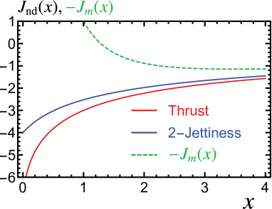
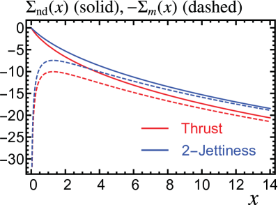
Figure 5: Massive corrections to the jet function. Panels (a) and (b) show the differential and cumulative jet functions, respectively. We show with solid lines the non-distributional functions $J_{\rm nd}$ and $\Sigma_{\rm nd}$ for P- (red) and M- (blue) schemes. The differential $J_{m}$ function is shown multiplied $-1$ as a green dashed line in panel (a) (for $x>0$ it is common to both schemes), while $-\Sigma_{m}$ is shown in panel (b) with red and blue dashed lines for P- and M-schemes, respectively.

Adding together the contributions from real and virtual corrections one obtains the complete jet function. The divergences are now entirely of UV origin and can be renormalized multiplicatively (with a convolution). Since in either massive scheme these are the same as for massless quarks, the renormalization factor is identical, along with the anomalous dimension. Therefore we quote directly the result for the renormalized jet functions [ $\alpha_{s}\equiv\alpha_{s}(\mu)$ ]:

$$J_{n}^{P}(s,\mu)=\, \delta(s)+\frac{\alpha_{s}C_{F}}{4\pi}\biggl{\{}\!\biggl{[}2\log\Bigl{(}\frac{m}{\mu}\Bigr{)}+8\log^{2}\Bigl{(}\frac{m}{\mu}\Bigr{)}\!+4+\frac{\pi^{2}}{3}\biggr{]}\delta(s)\!+\frac{8}{\mu^{2}}\biggl{[}\frac{\log(s/\mu^{2})}{s/\mu^{2}}\biggr{]}_{+}$$

$$-\!\frac{4}{\mu^{2}}\biggl{[}1+2\log\Bigl{(}\frac{m}{\mu}\Bigr{)}\biggr{]}\!\biggl{(}\frac{\mu^{2}}{s}\biggr{)}_{\!\!+}\!+\frac{s-7m^{2}}{(s-m^{2})^{2}}-\frac{2s(2s-5m^{2})}{(s-m^{2})^{3}}\log\Bigl{(}\frac{s}{m^{2}}\Bigr{)}\!\biggr{\}},$$

$$J_{n}^{J}(s+m^{2},\mu)=\, \delta(s)+\frac{\alpha_{s}C_{F}}{4\pi}\biggl{\{}\!\biggl{[}2\log\Bigl{(}\frac{m}{\mu}\Bigr{)}+8\log^{2}\Bigl{(}\frac{m}{\mu}\Bigr{)}\!+8-\frac{\pi^{2}}{3}\biggr{]}\delta(s)\!+\frac{8}{\mu^{2}}\biggl{[}\frac{\log(s/\mu^{2})}{s/\mu^{2}}\biggr{]}_{+}$$

$$-\!\frac{4}{\mu^{2}}\biggl{[}1+2\log\Bigl{(}\frac{m}{\mu}\Bigr{)}\biggr{]}\!\biggl{(}\frac{\mu^{2}}{s}\biggr{)}_{\!\!+}\!+\frac{s}{(m^{2}+s)^{2}}-\frac{4}{s}\log\Bigl{(}1+\frac{s}{m^{2}}\Bigr{)}\!\biggr{\}}.$$ (74)

From these equations one can easily read out the functional form of $J_{\rm nd}(x)$ defined in Eq. (28). With some manipulations one can also figure out expressions for $J_{m}(x)$ defined in the same equation:

$$J_{m}(x)=\, A_{S}\,\delta(x)-\biggl{(}\frac{1}{x}\biggr{)}_{\!\!+}+4\biggl{[}\frac{\log(x)}{x}\biggr{]}_{+}\,,$$

$$J_{\rm nd}^{J}(x)=\, \frac{x}{(x+1)^{2}}-\frac{4}{x}\log(1+x)\,,$$ (75)

$$J_{\rm nd}^{P}(x)=\, \frac{x-7}{(x-1)^{2}}-\frac{2x(2x-5)}{(x-1)^{3}}\log(x)\,,$$

with $A_{J}=2\pi^{2}/3+1$ and $A_{P}=4\pi^{2}/3-3$. We shall see that $J_{\rm nd}(x\to\infty)=-J_{m}(x)$ for both schemes, and show this behavior graphically in Fig. 5. This is expected since it corresponds to taking the massless limit, and therefore mass corrections should vanish such that the jet function becomes equal to the (renormalized) massless result of Eq. (68). Since $J_{\rm nd}$ contains distributions in this limit, it is advantageous to work with the cumulative jet function

$$\Sigma_{n}(s_{c})\equiv\!\int_{0}^{s_{c}}\!{\rm d}s\,J_{n}(s)\,,$$ (76)

which is a regular function. Likewise, one can define the cumulative functions for $J_{\rm nd}$ and $J_{m}$, which are also shown in Fig. 5. The result can be obtained easily and involves polylogarithms:

$$\Sigma_{n}^{J}(s+m^{2},\mu)=\, 1+\frac{\alpha_{s}C_{F}}{4\pi}\biggl{\{}2\log\Bigl{(}\frac{m}{\mu}\Bigr{)}+8\log^{2}\Bigl{(}\frac{m}{\mu}\Bigr{)}+8-\frac{\pi^{2}}{3}+\log\Bigl{(}1+\frac{s}{m^{2}}\Bigr{)}-\frac{s}{s+m^{2}}$$

$$+\,4\log^{2}\Bigl{(}\frac{s}{\mu^{2}}\Bigr{)}-4\biggl{[}1+2\log\Bigl{(}\frac{m}{\mu}\Bigr{)}\biggr{]}\!\log\Bigl{(}\frac{s}{\mu^{2}}\Bigr{)}+4\,\text{Li}_{2}\Bigl{(}-\frac{s}{m^{2}}\Bigr{)}\biggr{\}},$$ (77)

$$\Sigma_{n}^{P}(s,\mu)=\, 1+\frac{\alpha_{s}C_{F}}{4\pi}\biggl{\{}2\log\Bigl{(}\frac{m}{\mu}\Bigr{)}+8\log^{2}\Bigl{(}\frac{m}{\mu}\Bigr{)}+4+\frac{\pi^{2}}{3}-4\biggl{[}1+2\log\Bigl{(}\frac{m}{\mu}\Bigr{)}\biggr{]}\!\log\Bigl{(}\frac{s}{\mu^{2}}\Bigr{)}$$

$$+4\log^{2}\Bigl{(}\frac{s}{\mu^{2}}\Bigr{)}+4\,\text{Li}_{2}\Bigl{(}1-\frac{s}{m^{2}}\Bigr{)}+\frac{3s}{s-m^{2}}+\frac{(s-4m^{2})s}{(s-m^{2})^{2}}\log\Bigl{(}\frac{s}{m^{2}}\Bigr{)}\biggr{\}}.$$

As expected, in the $m\to 0$ limit both results reduce to the (same) massless cumulative jet function

$$\Sigma_{n}^{m=0}(s,\mu)=1+\frac{\alpha_{s}(\mu)C_{F}}{4\pi}\biggl{[}7-\pi^{2}-3\log\Bigl{(}\frac{s}{\mu^{2}}\Bigr{)}+2\log^{2}\Bigl{(}\frac{s}{\mu^{2}}\Bigr{)}\biggr{]}.$$ (78)

To take the derivative one needs to recall that the jet function has support only for positive $s$, such that it is effectively proportional to an (implicit) Heaviside function $\theta(s)$. Using the following relations:

$$\frac{\text{d}\theta(x)}{\text{d}x}=\delta(x)\;,\qquad\frac{\text{d}}{\text{d}x}[\theta(x)\log^{n}(x)]=n\biggl{[}\frac{\log^{n-1}(x)}{x}\biggr{]}_{+},$$ (79)

one readily arrives at Eq. (68). For $s>0$ one can expand around $m=0$ to find the following compact series

$$J_{n}^{P}(s>0,\mu)=\, \frac{\alpha_{s}C_{F}}{4\pi}\frac{1}{s}\biggl{\{}4\log\Bigl{(}\frac{s}{\mu^{2}}\Bigr{)}\!-3+\sum_{i=1}\biggl{[}1-6i-(4+i-3i^{2})\log\Bigl{(}\frac{s}{m^{2}}\Bigr{)}\!\biggr{]}\!\biggl{(}\frac{m^{2}}{s}\biggr{)}^{\!\!i}\,\biggr{\}}\,,$$

$$J_{n}^{J}(s>0,\mu)=\, \frac{\alpha_{s}C_{F}}{4\pi}\frac{1}{s}\biggl{\{}4\log\Bigl{(}\frac{s}{\mu^{2}}\Bigr{)}\!-3+\sum_{i=1}(-1)^{i}\biggr{(}i+1+\frac{4}{i}\biggl{)}\!\biggl{(}\frac{m^{2}}{s}\biggr{)}^{\!\!i}\,\biggr{\}}\,,$$ (80)

with similar results for the cumulative jet functions. Since individual pieces of the P-scheme thrust jet function have divergences at $s=m^{2}$ it is convenient to compute the expansion of $J^{P}_{\rm nd}(x)$ around $x=1$, which can be cast as

$$J_{\rm nd}^{P}(x)=-2\sum_{i=0}(1-x)^{i}\frac{9+5i}{(i+1)(i+2)(i+3)}\,.$$ (81)

6 Fixed-order Prediction in SCET

Inserting our result for the jet function into the SCET factorization theorem of Eq. (20), setting all renormalization scales equal and using the known results for the hard and soft function at one loop

$$H(Q,\mu)=\, 1+\frac{\alpha_{s}(\mu)C_{F}}{4\pi}\biggl{[}\frac{7\pi^{2}}{3}-16+12\log\biggl{(}\frac{Q}{\mu}\biggr{)}-8\log^{2}\biggl{(}\frac{Q}{\mu}\biggr{)}\biggr{]},$$ (82)

$$S(\ell,\mu)=\, \delta(\ell)+\frac{\alpha_{s}(\mu)C_{F}}{4\pi}\biggl{\{}\frac{\pi^{2}}{3}\delta(\ell)-\frac{16}{\mu}\biggl{[}\frac{\mu\log(\ell/\mu)}{\ell}\biggr{]}_{+}\biggr{\}},$$

one arrives at the fixed-order prediction for the partonic singular terms of the P-scheme thrust differential cross section: 

$$\frac{1}{\sigma_{0}}\frac{\text{d}\hat{\sigma}^{\rm SCET}_{\rm FO}}{\text{d}\tau}=\, \delta(\tau)+\frac{\alpha_{s}(\mu)C_{F}}{4\pi}F^{\rm SCET}_{1}(\tau,\hat{m})+\mathcal{O}(\alpha_{s}^{2})$$ (83)

$$F^{\rm SCET}_{1}(\tau,\hat{m})=\, \delta(\tau)\!\biggl{[}\frac{10\pi^{2}}{3}-8+4\log(\hat{m})+16\log^{2}(\hat{m})\biggr{]}-8[1+2\log(\hat{m})]\biggl{(}\frac{1}{\tau}\biggr{)}_{\!\!+}$$

$$\!\!\!+\frac{2(\tau-7\hat{m}^{2})}{(\tau-\hat{m}^{2})^{2}}-\frac{4\tau(2\tau-5\hat{m}^{2})}{(\tau-\hat{m}^{2})^{3}}\log\Bigl{(}\frac{\tau}{\hat{m}^{2}}\Bigr{)}$$

$$\equiv\, A^{\rm SCET}({\hat{m}})\delta(\tau)+B^{\rm SCET}_{\rm plus}({\hat{m}})\biggl{(}\frac{1}{\tau}\biggr{)}_{\!\!+}+F_{\rm NS}^{\rm SCET}(\tau,\hat{m})\,.$$

In the same way, one can get a similar expression for the cumulative distribution $\Sigma_{P}^{\rm SCET}$, which is among other things useful to take the $m\to 0$ limit. The differential cross section has a similar structure in full QCD, although it is different for vector and axial-vector currents as discussed in Ref. Lepenik:2019jjk , and for P-scheme thrust takes the following form 

$$\frac{1}{\sigma^{C}_{0}}\frac{\mathrm{d}\hat{\sigma}^{C}_{\rm FO}}{\mathrm{d}\tau}=\, R_{0}^{C}(\hat{m})\,\delta(\tau)+C_{F}\frac{\alpha_{s}}{\pi}F^{\rm QCD}_{C}(\tau,\hat{m})+\mathcal{O}(\alpha_{s}^{2})\,,$$ (84)

$$F^{\rm QCD}_{C}(\tau,\hat{m})=\, A^{C}({\hat{m}})\delta(\tau)+B^{C}_{\rm plus}({\hat{m}})\biggl{(}\frac{1}{\tau}\biggr{)}_{\!\!+}+F_{\rm NS}^{C}(\tau,\hat{m})\,,$$

where $C=V,A$ labels the type of current and with $R^{C}_{0}$ the tree-level massive R-ratio. Analytic results for $A^{C}$ and $B_{C}^{\rm plus}$ can be found in Ref. Lepenik:2019jjk and we quote here the universal value for the latter:

$$B^{C}_{\rm plus}(\hat{m})=\binom{3-\beta^{2}}{2\beta^{2}}\!\biggl{[}(1+\beta^{2})\log\biggl{(}\frac{1+\beta}{2\hat{m}}\biggr{)}-\beta\biggl{]},$$ (85)

with $\beta=\sqrt{1-4\hat{m}^{2}}$, and where the first and second line of the expression in big parentheses correspond to the vector and axial-vector currents, respectively. One recovers the SCET result for small masses, $A^{C}(\hat{m}\to 0)=A^{\rm SCET}(\hat{m})$ and $B_{\rm plus}^{C}(\hat{m}\to 0)=B_{\rm plus}^{\rm SCET}(\hat{m})$, and also

$$\lim_{\tau\to 0}F_{\rm NS}^{C}\Bigl{(}\tau,\hat{m}=\alpha\sqrt{\tau}\,\Bigr{)}\to F_{\rm NS}^{\rm SCET}\Bigl{(}\tau,\hat{m}=\alpha\sqrt{\tau}\,\Bigr{)},$$ (86)

with $\alpha\sim\mathcal{O}(1)$. Since for thrust $F_{\rm NS}^{C}$ is only known numerically, in Fig. 6 we show a comparison of QCD and SCET results for the NLO corrections scaling the mass as indicated in Eq. (86). Excellent numerical agreement is found as $\tau\to 0$ for various values of $\alpha$ between $1.2$ and $15$. We show only the vector current as for small values of $\tau$ it is indistinguishable from the axial-vector one.

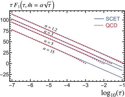
Figure 6: Comparison of the $\mathcal{O}(\alpha_{s})$ correction to the differential cross sections in QCD [ $F^{\rm QCD}_{V}(\tau,\hat{m})$ ] and SCET [ $F^{\rm SCET}_{1}(\tau,\hat{m})$ ]. We enforce the SCET power counting by scaling the reduced mass as $\hat{m}=\alpha\sqrt{\tau}$, with $\alpha=\mathcal{O}(1)$. Solid blue lines show SCET analytic results, while red dots correspond to QCD numerical predictions obtained from the computations in Ref. Lepenik:2019jjk . The numerical values of $\alpha$ are shown in the figure.

7 bHQET Jet Function Computation

The computation of the bHQET jet function is significantly simpler than for the SCET counterpart since in this EFT the mass is no longer a dynamical scale and we are left with tadpole-like integrals. As an immediate consequence of that, much as it happened for the massless SCET jet function, all virtual graphs are automatically zero in dimensional regularization since they are scaleless (this includes the wave-function renormalization factor). We are then left with the tree-level, which is common for both massive schemes, and real-radiation diagrams. The collinear event-shape measurements are the same in SCET and bHQET, although the contribution of massive particles needs to be power expanded, such that using $p=mv+k$ we obtain for thrust and 2-jettiness the following results

$$Q(\tau^{J}_{n}-\hat{m}^{2})=\, p^{+}\!-\frac{m^{2}}{Q}=mv_{+}\!-\frac{m^{2}}{Q}+k^{+}=k^{+}\,,$$ (87)

$$Q\tau^{P}_{n}=\, p^{+}\!-\frac{m^{2}}{p^{-}}=k^{+}\!+\frac{m^{2}}{Q}-\frac{m^{2}}{Q+k^{-}}=k^{+}\!+\hat{m}^{2}k^{-}=0\,,$$

where to get to the third equality of the second line we have used $Q\gg k^{-}$ [ as can be seen from Eq. (33) ], and to obtain $\tau_{n}^{P}=0$ we use the on-shell condition for heavy quarks $v\cdot k=0$, to be discussed later in this section. The field-theoretical definition of the bHQET jet function can be obtained from the expression given in Eq. (37), and taking into account that applying the bHQET power counting to the minus component of momenta one obtains $\delta(\mathcal{\bar{P}}-Q)\to\delta(k^{-}+\sum q^{-})$, with $q$ representing momenta of particles other than the heavy quark, the jet functions can be written as

$$B_{n}(\hat{s})=\frac{(2\pi)^{d-1}Q}{2m^{2}N_{C}}\mathrm{Tr}\langle 0|W_{v_{+}}^{\dagger}\!(0)h_{v_{+}}\!(0)\delta\!\biggl{[}\hat{s}-\frac{Q^{2}}{m}(\hat{e}_{n}-e_{\rm min})\biggr{]}\delta^{(d-2)}(\vec{\mathcal{K}}^{\perp})\delta(\mathcal{K}^{-})\bar{h}_{v_{+}}\!(0)W_{v_{+}}\!(0)|0\rangle.$$ (88)

Here $\vec{\mathcal{K}}$ is an operator that pulls out the residual momenta of the heavy quarks and the (full) momenta of ultra-collinear particles. We have also used $\vec{v}_{\perp}=\vec{0}$ and $W_{v_{+}}$ has the same functional form as $W_{n}$ replacing the collinear gluons by ultra-collinear fields: $A_{n}\rightarrow A_{+}$:

$$W_{v_{+}}(x) \equiv\bar{P}\exp\biggl{[}-ig\!\!\int_{0}^{\infty}\!\mathrm{d}s\,\,\,\bar{n}\cdot\!A_{+}(\bar{n}\,s+x)\biggr{]},$$ (89)

$$W_{v_{+}}^{\dagger}(x) \equiv P\exp\biggl{[}ig\!\!\int_{0}^{\infty}\!\mathrm{d}s\,\,\,\bar{n}\cdot\!A_{+}(\bar{n}\,s+x)\biggr{]}.$$

The bHQET phase-space integration involving a heavy quark gets also simplified, and using again $p=mv+k$ one has that

$$\frac{{\rm d}^{d}p}{(2\pi)^{d-1}}\,\delta(p^{2}-m^{2})\theta(p^{0})=\, \frac{{\rm d}p^{+}{\rm d}p^{-}{\rm d}^{d-2}\vec{p}_{\perp}}{2(2\pi)^{d-1}}\,\delta\bigl{[}p^{-}p^{+}-|\vec{p}_{\perp}|^{2}-m^{2}\bigr{]}\theta(p^{-}+p^{+})$$ (90)

$$=\, \frac{{\rm d}k^{+}{\rm d}k^{-}{\rm d}^{d-2}\vec{k}_{\perp}}{2(2\pi)^{d-1}}\,\delta\Bigl{(}Qk^{+}+\frac{m^{2}}{Q}k^{-}+k^{2}\Bigr{)}\theta\Bigl{(}Q+k^{-}\!+\frac{m^{2}}{Q}+k^{+}\Bigr{)}$$

$$=\, \frac{{\rm d}k^{+}{\rm d}k^{-}{\rm d}^{d-2}\vec{k}_{\perp}}{2(2\pi)^{d-1}}\,\delta\Bigl{(}Qk^{+}+\frac{m^{2}}{Q}k^{-}\!\Bigr{)}\theta(Q)=\frac{{\rm d}k^{-}{\rm d}^{d-2}\vec{k}_{\perp}}{2Q(2\pi)^{d-1}}\,,$$

where in the second line we have used Eq. (33) and in the third we power-count away the $k^{2}$ in the delta function argument along with all terms but $Q$ inside the Heaviside function. The on-shell condition for heavy quarks written in light-cone coordinates implies $v^{-}k^{+}+k^{-}v^{+}=0$, in agreement with the argument of the delta function. When comparing to Eq. (41) we observe that the $p^{-}$ in the denominator got replaced by $Q$ and that the $p^{-}$ integration is not limited to positive values only. The phase-space integration for ultracollinear particles stays the same as in SCET.

Feynman diagrams look exactly the same in SCET and bHQET, with the replacement $p\to k$ for the heavy quark momenta. Let us compute the tree-level contribution as given in Fig. 2, which is analogous to the corresponding SCET calculation:

$$mB_{n}^{\rm tree}(s)=\!\!\int\!\frac{{\rm d}k^{-}\!}{4m}{\rm d}^{d-2}\vec{k}_{\perp}\delta^{(d-2)}(\vec{k}_{\perp})\delta(k^{-})\delta\!\biggl{[}\hat{s}-\frac{Q^{2}}{m}(\hat{e}_{n}-e_{\rm min})\biggr{]}\!\sum_{s}{\rm Tr}\bigl{[}u_{s}(p)\overline{u}_{s}(p)\bigr{]}=\delta(\hat{s})\,,$$ (91)

where we have used that the trace of the polarization sum equals $4m$ and have integrated all delta functions except the one with the measurement. The condition $k^{-}=0$ imposed by the Dirac delta function makes both (shifted) measurements coincide at tree-level, see Eq. (87). There are some generic features to be learned from this diagram: since there is no Dirac structure in the diagram, the trace of the polarization sum will be always $4m$ at any loop order, and since there is always one heavy quark which brings an inverse power of $Q$ through its phase space one has the following combination:

$$\frac{Q}{2m}\frac{1}{2Q}{\rm Tr}\bigl{[}u_{s}(p)\overline{u}_{s}(p)\bigr{]}=1\,,$$ (92)

which eliminates the spurious dependence on $m$ and $Q$, ultraviolet scales that should not appear in EFT computations. To make this non-dependence explicit at higher orders one can rescale the minus component of ultracollinear real particles as $q_{i}^{-}=(Q/m)\ell_{i}$, as we shall do in the rest of the section.

We turn our attention now to real-radiation contributions, for which we can simplify the heavy-quark propagator using $v\cdot k=0$. We start with diagram (a) of Fig. 4, that after applying the bHQET Feynman rules becomes

$$mB_{a}^{\rm real}(\hat{s},\mu)=\frac{2\alpha_{s}C_{F}(\mu^{2}e^{\gamma_{E}})^{\varepsilon}}{\pi\Gamma(1-\varepsilon)}\!\int\!\!\frac{{\rm d}\ell^{-}}{(\ell^{-})^{2}}\frac{|\vec{q}_{\perp}|^{1-2\varepsilon}{\rm d}|\vec{q}_{\perp}|}{v\!\cdot\!q}\theta(\ell^{-})\delta\!\biggl{[}\hat{s}-\frac{Q^{2}}{m}(\hat{e}_{n}-e_{\rm min})\biggr{]}.$$ (93)

The on-shell condition on the ultra-collinear gluon momenta implies in light-cone coordinates: $2\,v\!\cdot\!q=|\vec{q}_{\perp}|^{2}Q/(mq^{-})+mq^{-}/Q=[\,|\vec{q}_{\perp}|^{2}+(\ell^{-})^{2}\,]/\ell^{-}$. For diagram (c) we get instead

$$mB_{c}^{\rm real}(\hat{s},\mu)=-\frac{\alpha_{s}C_{F}(\mu^{2}e^{\gamma_{E}})^{\varepsilon}}{2\pi\Gamma(1-\varepsilon)}\!\int\!\frac{{\rm d}\ell^{-}}{\ell^{-}}\frac{|\vec{q}_{\perp}|^{1-2\varepsilon}{\rm d}|\vec{k}_{\perp}|}{(v\!\cdot\!q)^{2}}\theta(\ell^{-})\delta\!\biggl{[}\hat{s}-\frac{Q^{2}}{m}(\hat{e}_{n}-e_{\rm min})\biggr{]}.$$ (94)

Let us work out the measurements for thrust and 2-jettiness

$$\frac{Q^{2}}{m}(\tau^{J}_{n}-\hat{m}^{2})=\, \frac{Q}{m}(q^{+}+k^{+})=\frac{Q}{m}\frac{|\vec{q}_{\perp}|^{2}}{q^{-}}+\frac{m}{Q}q^{-}=\frac{|\vec{q}_{\perp}|^{2}}{\ell^{-}}+\ell^{-}\,,$$ (95)

$$\frac{Q^{2}}{m}\tau^{P}_{n}=\, \frac{Q}{m}q^{+}=\frac{Q}{m}\frac{|\vec{q}_{\perp}|^{2}}{q^{-}}=\frac{|\vec{q}_{\perp}|^{2}}{\ell^{-}}\,,$$

where we have used Eq. (87), the on-shell condition for heavy quarks and ultra-collinear massless gluons, and the fact that label momentum conservation implies $k^{-}=-q^{-}$. With this result it is very simple to solve the measurement delta function in terms of the perpendicular gluon momenta

$$\delta\!\biggl{[}\hat{s}-\frac{Q^{2}}{m}(\tau^{J}_{n}-\hat{m}^{2})\biggr{]}=\, \frac{\ell^{-}}{2|\vec{q}_{\perp}|}\,\delta\!\Bigl{[}|\vec{q}_{\perp}|-\sqrt{\hat{s}\,\ell^{-}-(\ell^{-})^{2}}\,\Big{]},$$ (96)

$$\delta\biggl{(}\hat{s}-\frac{Q^{2}}{m}\tau^{P}_{n}\biggr{)}=\, \frac{\ell^{-}}{2|\vec{q}_{\perp}|}\,\delta\Bigl{(}|\vec{q}_{\perp}|-\sqrt{\hat{s}\,\ell^{-}}\,\Bigr{)},$$

and we will use these results to compute the jet functions in the next two sub-sections.

7.1 Thrust

We start with the diagram in which the gluon is radiated from the Wilson line. Switching variables to $\ell^{-}=\hat{s}x$ we arrive at

$$mB_{a,P}^{\rm real}(\hat{s},\mu)=\, \frac{\alpha_{s}(\mu^{2}e^{\gamma_{E}})^{\varepsilon}C_{F}}{2\pi}\frac{\hat{s}^{\,-1-2\varepsilon}}{\Gamma(1-\varepsilon)}\int_{0}^{\infty}{\rm d}x\,\frac{x^{-1-\varepsilon}}{1+x}=-\frac{\alpha_{s}\Gamma(1+\varepsilon)C_{F}\,e^{\varepsilon\gamma_{E}}}{2\pi\mu^{2}\varepsilon}\biggl{(}\frac{\hat{s}}{\mu^{2}}\biggr{)}^{\!\!-1-2\varepsilon}$$

$$=\, \frac{\alpha_{s}C_{F}}{4\pi}\biggl{[}\biggl{(}\frac{1}{\varepsilon^{2}}+\frac{\pi^{2}}{12}\biggr{)}\delta(\hat{s})-\frac{2}{\varepsilon\mu}\biggl{(}\frac{\mu}{\hat{s}}\biggr{)}_{\!\!+}+\frac{4}{\mu}\biggl{(}\frac{\mu\log(\hat{s}/\mu)}{\hat{s}}\biggr{)}_{\!\!+}\,\biggr{]}.$$ (97)

With an identical change of variables we arrive at the following result for diagram (c):

$$mB_{c,P}^{\rm real}(\hat{s},\mu)= -\!\frac{\alpha_{s}(\mu^{2}e^{\gamma_{E}})^{\varepsilon}C_{F}}{\pi}\frac{\hat{s}^{\,-1-2\varepsilon}}{\Gamma(1-\varepsilon)}\int_{0}^{\infty}{\rm d}x\,\frac{x^{-\varepsilon}}{(1+x)^{2}}$$ (98)

$$= -\!\frac{\alpha_{s}\Gamma(1+\varepsilon)C_{F}\,e^{\varepsilon\gamma_{E}}}{\pi\mu^{2}}\biggl{(}\frac{\hat{s}}{\mu^{2}}\biggr{)}^{\!\!-1-2\varepsilon}=\frac{\alpha_{s}C_{F}}{4\pi}\biggl{[}\frac{2}{\varepsilon}\,\delta(\hat{s})-\frac{4}{\mu}\biggl{(}\frac{\mu}{\hat{s}}\biggr{)}_{\!\!+}\,\biggr{]}.$$

Adding both diagrams with the appropriate factors we obtain the final expression for the P-scheme hemisphere jet function:

$$mB_{n}^{P}(\hat{s},\mu)=\, \!-\!\frac{\alpha_{s}\Gamma(2+\varepsilon)C_{F}\,e^{\varepsilon\gamma_{E}}}{\pi\mu^{2}\varepsilon}\biggl{(}\frac{\hat{s}}{\mu^{2}}\biggr{)}^{\!\!-1-2\varepsilon}$$ (99)

$$=\, \frac{\alpha_{s}C_{F}}{4\pi}\biggl{[}\biggl{(}\frac{2}{\varepsilon^{2}}+\frac{2}{\varepsilon}+\frac{\pi^{2}}{6}\biggr{)}\delta(\hat{s})-\frac{4}{\mu}\biggl{(}\frac{1}{\varepsilon}+1\biggr{)}\!\biggl{(}\frac{\mu}{\hat{s}}\biggr{)}_{\!\!+}+\frac{8}{\mu}\biggl{(}\frac{\mu\log(\hat{s}/\mu)}{\hat{s}}\biggr{)}_{\!\!+}\,\biggr{]}.$$

7.2 Jettiness

The Dirac delta function in Eq. (96) implies that there is a solution for $|\vec{q}_{\perp}|$ only if $\ell^{-}<\hat{s}$, which can be implemented through a Heaviside function and bounds the upper integration limit for $\ell^{-}$. With the change of variables implemented in the previous section the integration limits are mapped to the interval $(0,1)$ and we get the following result for diagram (a):

$$mB_{a,J}^{\rm real}(\hat{s},\mu)=\, \frac{\alpha_{s}(\mu^{2}e^{\gamma_{E}})^{\varepsilon}C_{F}}{2\pi}\frac{\hat{s}^{\,-1-2\varepsilon}}{\Gamma(1-\varepsilon)}\!\!\int_{0}^{1}\!\!{\rm d}x\,x^{-1-\varepsilon}(1-x)^{-\varepsilon}$$

$$= -\!\frac{\alpha_{s}\Gamma(1-\varepsilon)C_{F}e^{\varepsilon\gamma_{E}}}{2\pi\mu^{2}\varepsilon\Gamma(1-2\varepsilon)}\biggl{(}\frac{\hat{s}}{\mu^{2}}\biggr{)}^{\!\!-1-2\varepsilon}$$ (100)

$$=\, \frac{\alpha_{s}C_{F}}{4\pi}\biggl{[}\biggl{(}\frac{1}{\varepsilon^{2}}-\frac{\pi^{2}}{4}\biggr{)}\delta(\hat{s})-\frac{2}{\varepsilon\mu}\biggl{(}\frac{\mu}{\hat{s}}\biggr{)}_{\!\!+}+\frac{4}{\mu}\biggl{(}\frac{\mu\log(\hat{s}/\mu)}{\hat{s}}\biggr{)}_{\!\!+}\,\biggr{]},$$

that, as expected, differs from the expression in Eq. (7.1) only in the non-divergent term of the delta-function coefficient. Similarly, we obtain for diagram (c)

$$mB_{c,J}^{\rm real}(\hat{s},\mu)=\, \!-\!\frac{\alpha_{s}(\mu^{2}e^{\gamma_{E}})^{\varepsilon}C_{F}}{\pi}\frac{\hat{s}^{\,-1-2\varepsilon}}{\Gamma(1-\varepsilon)}\!\int_{0}^{1}\!{\rm d}x\,[x(1-x)]^{-\varepsilon}\!$$ (101)

$$=\, \!-\frac{\alpha_{s}\Gamma(1-\varepsilon)C_{F}\,e^{\varepsilon\gamma_{E}}}{\pi\mu^{2}\Gamma(2-2\varepsilon)}\biggl{(}\frac{\hat{s}}{\mu^{2}}\biggr{)}^{\!\!-1-2\varepsilon}=\frac{\alpha_{s}C_{F}}{4\pi}\biggl{[}2\biggl{(}\frac{1}{\varepsilon}+2\biggr{)}\,\delta(\hat{s})-\frac{4}{\mu}\biggl{(}\frac{\mu}{\hat{s}}\biggr{)}_{\!\!+}\,\biggr{]},$$

again almost identical to the corresponding P-scheme computation. Adding twice the first diagram plus the second we recover the known result for the 2-jettiness bHQET jet function:

$$mB_{n}^{J}(\hat{s},\mu)=\, \!-\!\frac{\alpha_{s}\Gamma(2-\varepsilon)C_{F}\,e^{\varepsilon\gamma_{E}}}{\pi\mu^{2}\varepsilon\Gamma(2-2\varepsilon)}\biggl{(}\frac{\hat{s}}{\mu^{2}}\biggr{)}^{\!\!-1-2\varepsilon}$$ (102)

$$=\, \frac{\alpha_{s}C_{F}}{4\pi}\biggl{[}\biggl{(}\frac{2}{\varepsilon^{2}}+\frac{2}{\varepsilon}+4-\frac{\pi^{2}}{2}\biggr{)}\delta(\hat{s})-\frac{4}{\varepsilon\mu}\biggl{(}\frac{1}{\varepsilon}+1\biggr{)}\!\biggl{(}\frac{\mu}{\hat{s}}\biggr{)}_{\!\!+}+\frac{8}{\mu}\biggl{(}\frac{\mu\log(\hat{s}/\mu)}{\hat{s}}\biggr{)}_{\!\!+}\,\biggr{]}.$$

Both schemes have the same divergent structure and hence their anomalous dimension, as expected, are identical. Furthermore, the difference between the respective delta coefficients is the same as that in the SCET jet functions. This result was also expected since both theories should smoothly match in the bHQET limit.

8 RG Evolution of the SCET Jet Function

In this section we solve the renormalization group equation for the non-distributional part of the jet function for thrust and 2-jettiness. This amounts to finding an analytic expression for the function $I_{\rm nd}$ defined in the last line of Eq. (4.1). Even though the result for $I^{J}_{\rm nd}$ has been already worked out in Ref. Fleming:2007xt , we present here the main steps to find the solution as they are illustrative. Using the rightmost integral expression of the bottom line in Eq. (4.1) we find

$$I^{J}_{\rm nd}(\tilde{\omega},y)=\frac{1}{\Gamma(-\tilde{\omega})}\int_{0}^{1}{\rm d}z\,(1-z)^{-1-\tilde{\omega}}\biggl{[}\frac{zy}{(1+zy)^{2}}-\frac{4\log(1+zy)}{zy}\biggr{]}.$$ (103)

While the first term on the right-hand side of Eq. (103) is already in a canonical form such that Eq. (56) can be directly applied, the second contains a logarithm. Expressing it as an integral

$$\frac{\log(1+zy)}{zy}=\int_{0}^{1}\mathrm{d}x\,\frac{1}{1+xzy}\,,$$ (104)

brings the second term also into a canonical form that we can easily integrate, finding

$$\int_{0}^{1}\mathrm{d}z(1-z)^{-1-\tilde{\omega}}\,\frac{\log(1+zy)}{zy}=\!\int_{0}^{1}\!\mathrm{d}x\!\int_{0}^{1}\!\mathrm{d}z(1-z)^{-1-\tilde{\omega}}\frac{1}{1+xzy}$$ (105)

$$\qquad\qquad=-\frac{1}{\tilde{\omega}}\!\int_{0}^{1}\!\mathrm{d}x\,{}_{2}F_{1}(1,1,1-\tilde{\omega},-xy)=-\frac{1}{\tilde{\omega}}\,_{3}F_{2}(1,1,1,2,1-\tilde{\omega},-y),$$

where in the last step we have used the integral representation of the ${}_{3}F_{2}$ function:

$$_{3}F_{2}(a_{1},a_{2},a_{3},b_{1},b_{2},z)=\frac{\Gamma(b_{2})}{\Gamma(a_{3})\Gamma(b_{2}-a_{3})}\!\int_{0}^{1}\!\mathrm{d}t\,t^{a_{3}-1}(1-t)^{b_{2}-1-a_{3}}\,{}_{2}F_{1}(a_{1},a_{2},b_{1},tz)\,,$$ (106)

with $a_{1}=a_{2}=a_{3}=1$, $b_{1}=1-\tilde{\omega}$ and $b_{2}=2$. After adding the result for the first term we find an expression slightly simpler than that quoted in Ref. Fleming:2007xt , although fully equivalent:

$$I^{J}_{\rm nd}(\tilde{\omega},y)=\frac{1}{\Gamma(2-\tilde{\omega})}\bigl{[}y\,_{2}F_{1}(2,2,2-\tilde{\omega},-y)-(1-\tilde{\omega})\,_{3}F_{2}(1,1,1,2,1-\tilde{\omega},-y)\bigr{]}\,,$$ (107)

which has a smooth $\tilde{\omega}\to 0$ limit. For a numerical implementation, one can use standard routines to evaluate ${}_{2}F_{1}$ hypergeometric functions in programming languages such as Mathematica, Fortran, Python, or C++. For ${}_{3}F_{2}$ there are built-in routines in Mathematica and Python, while for other languages one can use a numerical integration over ${}_{2}F_{1}$ as shown in Eq. (106).

For P-scheme thrust we can write the logarithm as a derivative to bring all terms into a canonical form:

$$I^{P}_{\rm nd}(\tilde{\omega},y)=\, \frac{1}{\Gamma(-\tilde{\omega})}\!\int_{0}^{1}\mathrm{d}z(1-z)^{-1-\tilde{\omega}}\left[\frac{zy-7}{(1-yz)^{2}}+\frac{2zy(2zy-5)}{(1-yz)^{3}}\log(zy)\right]$$ (108)

$$\frac{1}{\Gamma(-\tilde{\omega})}\!\int_{0}^{1}\!{\rm d}z\,(1-z)^{-1-\tilde{\omega}}\biggl{\{}\!\frac{zy-7}{(1-yz)^{2}}+\frac{2yz(2zy-5)}{(1-yz)^{3}}\biggl{[}\log(y)+\frac{\rm d}{{\rm d}\varepsilon}z^{\varepsilon}\biggr{]}\!\biggr{\}}_{\varepsilon\to 0}.$$

For $y>1$ each one of the terms in the integral diverges when $z=1/y$. We can regularize the divergence adding a small imaginary part $y\to y+i\epsilon$. This makes each integral complex, although the sum is real when $\epsilon\to 0$. To express our result in terms of a minimal set of hypergeometric functions, we use the following identity:

$$(c-b){}_{2}F_{1}(a,b-1,c,z) +(c-1)(z-1){}_{2}F_{1}(a,b,c-1,z)$$ (109)

$$+[z(a-c+1)+b-1]{}_{2}F_{1}(a,b,c,z)=0.$$

Furthermore, one can use an additional identity to make the final result manifestly real also for the case $y>1$

$$_{2}F_{1}(a,b;c;z)=\, \frac{\Gamma(c)(1-z)^{c-a-b}\Gamma(a+b-c)\,{}_{2}F_{1}(c-a,c-b,1+c-a-b,1-z)}{\Gamma(a)\Gamma(b)}$$ (110)

$$+\frac{\Gamma(c)\Gamma(c-a-b)\,{}_{2}F_{1}(a,b,a+b-c+1,1-z)}{\Gamma(c-a)\Gamma(c-b)}.$$

After solving all integrals, recursively applying Eq. (109) and transforming the hypergeometric functions using Eq. (110), one arrives at the second important result of this article: 

$$I^{P}_{\rm nd}(\tilde{\omega},y)=\, \frac{4y^{2}-2(\tilde{\omega}+5)y-\tilde{\omega}(3\,\tilde{\omega}+7)}{(1-y)^{2}(1+\tilde{\omega})\Gamma(1-\tilde{\omega})}\biggl{\{}\tilde{\omega}\frac{{\rm d}}{{\rm d}\varepsilon}\,{}_{2}F_{1}(1,1+\varepsilon,2+\tilde{\omega},1-y)$$

$$\!\!\!\!\!+\!\bigg{(}\tilde{\omega}\log(y)-\tilde{\omega}H_{1-\tilde{\omega}}-\frac{1-2\tilde{\omega}}{1-\tilde{\omega}}\biggr{)}{}_{2}F_{1}(1,1,2+\tilde{\omega},1-y)\biggr{\}}_{\!\varepsilon\to 0}$$ (112)

$$\!\!\!\!-\!\frac{(1-\tilde{\omega})\tilde{\omega}(3\,\tilde{\omega}-y+7)[H_{1-\tilde{\omega}}-\log(y)]-\tilde{\omega}[3\,\tilde{\omega}(y+1)-5y+14]-y+7}{\Gamma(2-\tilde{\omega})(1-y)^{2}}\,,$$

with $H_{a}$ the harmonic number, which for non-integer values of $a$ can be expressed in terms of the digamma function: $H_{a}=\psi^{(0)}(1+a)+\gamma_{E}$. Equation (8) has been cast in a way in which the no-resummation limit $\tilde{\omega}\to 0$ is smooth. The singularities that appear in individual terms of $J^{P}_{\rm nd}$ for $x=1$ manifest themselves now as a double pole in $I^{P}_{\rm nd}$ at $y=1$, which is however fictitious, as the result is indeed smooth at this value. To solve this problem in numerical implementations we provide in Sec. 8.2 an expansion of this result around $y=1$ at an arbitrarily high order. The result in Eq. (8) is adequate for a numerical implementation since the derivative with respect to $\varepsilon$ can be taken numerically through finite differences. It can be also performed analytically, using Eq. (110) in ${}_{2}F_{1}(1,1+\varepsilon,2+\tilde{\omega},1-y)$ and the following identity

$$\frac{\text{d}}{\text{d}\varepsilon}{}_{2}F_{1}(1,1+\varepsilon,1-\tilde{\omega}+\varepsilon,y)\biggl{|}_{\varepsilon\rightarrow 0}\!\!=-\frac{\tilde{\omega}\,y(1-y)^{-1-\tilde{\omega}}}{(1-\tilde{\omega})^{2}}{}_{3}F_{2}(1-\tilde{\omega},1-\tilde{\omega},1-\tilde{\omega},2-\tilde{\omega},2-\tilde{\omega},y),$$ (113)

to arrive at the equivalent expression:

$$I^{P}_{\rm nd}(\tilde{\omega},y)=$$ (114)

$$\frac{\tilde{\omega}\,y(1-y)^{-3-\tilde{\omega}}[\,2\,y\,(\tilde{\omega}+5)+\tilde{\omega}(3\tilde{\omega}+7)-4y^{2}\,]\,{}_{3}F_{2}(1-\tilde{\omega},1-\tilde{\omega},1-\tilde{\omega},2-\tilde{\omega},2-\tilde{\omega},y)}{\Gamma(2-\tilde{\omega})(1-\tilde{\omega})}$$

$$-\frac{(1-\tilde{\omega})\,\tilde{\omega}\,(3\,\tilde{\omega}-y+7)[\,H_{1-\tilde{\omega}}-\log(y)\,]-\tilde{\omega}\,[\,3\,\tilde{\omega}\,(y+1)-5\,y+14\,]-y+7}{\Gamma(2-\tilde{\omega})(1-y)^{2}}$$

$$+\frac{[\,2\,y\,(\tilde{\omega}+5)+\tilde{\omega}\,(3\,\tilde{\omega}+7)-4y^{2}\,]\{(1-\tilde{\omega})[\,H_{1-\tilde{\omega}}-\log(y)\,]-1\}_{2}F_{1}(1,1,1-\tilde{\omega},y)}{\Gamma(2-\tilde{\omega})(1-y)^{2}}.$$

The $(1-y)^{-3-\tilde{\omega}}$ factor and both hypergeometric functions are complex for $y>1$ but the combination is real. To have all terms explicitly real for $y>1$ one can use the following relation

$$\frac{\text{d}}{\text{d}\varepsilon}{}_{2}F_{1}(1,1+\varepsilon,2+\tilde{\omega},1-y)\Bigr{|}_{\varepsilon\rightarrow 0}=\frac{1-y}{y^{2}(2+\tilde{\omega})^{2}}\,{}_{3}F_{2}\biggl{(}\!2,2+\tilde{\omega},2+\tilde{\omega},3+\tilde{\omega},3+\tilde{\omega},1-\frac{1}{y}\biggr{)}$$

$$\qquad+y^{\tilde{\omega}}(1-y)\frac{1+\tilde{\omega}}{(2+\tilde{\omega})^{2}}\,{}_{3}F_{2}(2+\tilde{\omega},2+\tilde{\omega},2+\tilde{\omega},3+\tilde{\omega},3+\tilde{\omega},1-y)\,,$$ (115)

which does not rely on numerical derivatives, is manifestly real for all positive values of $y$ but is numerically unstable if $y\to 0$. This poses no problem in practice, since for $y<1$ one can simply switch to Eq. (114). To derive the result in Eq. (8) we proceed as follows:

$$\frac{\text{d}}{\text{d}\varepsilon}{}_{2}F_{1}(1,1+\varepsilon,2+\tilde{\omega},1-y)\Bigr{|}_{\varepsilon\rightarrow 0}=-\frac{1}{y}\frac{\text{d}}{\text{d}b}{}_{2}F_{1}\!\biggl{(}1,b,2+\tilde{\omega},1-\frac{1}{y}\biggr{)}\biggl{|}_{b\rightarrow 1+\tilde{\omega}}$$

$$\qquad=\frac{1}{y}\frac{\text{d}}{\text{d}b}\biggl{[}{}_{2}F_{1}\biggl{(}1,1+\tilde{\omega},b+1,1-\frac{1}{y}\biggr{)}-{}_{2}F_{1}\biggl{(}1,b,b+1,1-\frac{1}{y}\biggr{)}\biggr{]}_{b\rightarrow 1+\tilde{\omega}}$$ (116)

$$\qquad=\frac{1}{y}\frac{\text{d}}{\text{d}b}\biggl{[}y^{1+\tilde{\omega}}{}_{2}F_{1}(b,1+\tilde{\omega},b+1,1-y)-{}_{2}F_{1}\biggl{(}1,b,b+1,1-\frac{1}{y}\biggr{)}\biggr{]}_{b\rightarrow 1+\tilde{\omega}}$$

where in the first step we have used Eq. (57), in the second we apply the chain rule on derivatives, and in the third line we use again Eq. (57) on the first term. Using the identity

$$\frac{\text{d}}{\text{d}a}\,{}_{2}F_{1}(a,b,a+1,z)=\frac{bz}{(a+1)^{2}}\,{}_{3}F_{2}(a+1,a+1,b+1,a+2,a+2,z)\,,$$ (117)

in the two terms of the last line in Eq. (8) we arrive at the result quoted in Eq. (8). In Appendix B we present an alternative (although more complicated) expression for $I^{P}_{\rm nd}$ which does not involve numerical derivatives and with every term manifestly real for $y>1$. We use this result as an additional cross check of our analytic derivations. In any case, we shall see that for numerical implementations one never needs to use expressions involving hypergeometric functions.

8.1 Expansion around $s=0$

For numerical implementation purposes, it might be convenient to obtain an analytic expansion of $I_{\rm nd}(\tilde{\omega},y)$ around $y=0$. One can do so by using the known expansions for the hypergeometric functions, e.g.

$$_{2}F_{1}(a,b,c,z)=\frac{\Gamma(c)}{\Gamma(a)\Gamma(b)}\sum_{i=0}^{\infty}\frac{\Gamma(a+i)\Gamma(b+i)}{\Gamma(c+i)\Gamma(i+1)}\,z^{i}\,,$$ (118)

but in order to have a relation valid at arbitrarily high orders it is simpler to use the expansion of $J_{\rm nd}(x)$ around $x=0$

$$J_{\rm nd}^{P}(x)=\, -\!\sum_{i=0}[\,6\,i+7+i(7+3i)\log(x)\,]\,x^{i}\,,$$ (119)

$$J_{\rm nd}^{J}(x)=\, -\!\sum_{i=0}\biggl{(}i+\frac{4}{i+1}\biggr{)}(-x)^{i}\,,$$

on the leftmost expression of the bottom line in Eq. (4.1) and integrate analytically term by term. It turns out that one can sum up the corresponding series using Eq. (118) to recover an expression analytically equivalent to Eq. (114). The master integrals that we will need are

$$\frac{y^{\tilde{\omega}}}{\Gamma(-\tilde{\omega})}\int_{0}^{y}\text{d}x\,(y-x)^{-1-\tilde{\omega}}x^{i}=\, y^{i}\frac{\Gamma(1+i)}{\Gamma(1+i-\tilde{\omega})}\,,$$ (120)

$$\frac{y^{\tilde{\omega}}}{\Gamma(-\tilde{\omega})}\int_{0}^{y}\text{d}x\,(y-x)^{-1-\tilde{\omega}}x^{i}\log(x)=\, y^{i}\frac{\Gamma(1+i)}{\Gamma(1+i-\tilde{\omega})}[H_{i}-H_{i-\tilde{\omega}}+\log(y)]\,,$$

where the bottom line can be obtained from the top one acting with a derivative with respect to $i$. We then arrive at

$$I^{P}_{\rm nd}(\tilde{\omega},y)=\, \!-\!\frac{1}{\Gamma(1-\tilde{\omega})}\!\sum_{i=0}\frac{i!}{(1-\tilde{\omega})_{i}}\{(6i+7)+i(7+3i)[H_{i}-H_{i-\tilde{\omega}}+\log(y)]\,\}\,y^{i}\,,$$ (121)

$$I^{J}_{\rm nd}(\tilde{\omega},y)=\, \!-\!\frac{1}{\Gamma(1-\tilde{\omega})}\!\sum_{i=0}\biggl{(}i+\frac{4}{i+1}\biggr{)}\frac{i!}{(1-\tilde{\omega})_{i}}(-y)^{i}\,.$$

where we have used the Pochhammer symbol $(a)_{n}\equiv\Gamma(a+n)/\Gamma(a)$ since it is convenient for an optimized numerical implementation. Both series converge well for $|y|<1$, and therefore apply mainly in the peak of the distribution. For 2-jettiness the series can be easily summed up using Eq. (118) and the series expansion for the ${}_{3}F_{2}$ hypergeometric function:

$${}_{3}F_{2}(a,b,c,d,e,z)=\frac{\Gamma(c)}{\Gamma(a)\Gamma(b)}\sum_{i=0}^{\infty}\frac{\Gamma(a+i)\Gamma(b+i)\Gamma(c+i)}{\Gamma(d+i)\Gamma(e+i)\Gamma(i+1)}\,z^{i}\,.$$ (122)

For P-scheme thrust one can convert the term involving harmonic numbers into the derivative of ratios of gamma functions to use Eq. (118) and recover the result we already obtained with a direct integration. The numerical implementation of Ref. Butenschoen:2016lpz (which dealt with 2-jettiness) did not use this expansion and the evaluation of the non-distributional jet function running was the most severe performance bottleneck for the code.

8.2 Expansion around $s=m^{2}$

The results obtained in Eqs. (8) and (114) are not useful for a numerical implementation in the vicinity of $y=1$. When $y$ is sufficiently close to unity one can switch to a series expansion to arbitrary high power using the change of variables $z\to 1-z$ in the rightmost expression at the bottom of Eq. (4.1) and the following expansion:

$$J_{\rm nd}^{P}[(1-z)(1+y)]=-\biggl{[}\frac{2(1-z)(3+2z)}{z^{3}}\log(1-z)+\frac{z+6}{z^{2}}\biggr{]}-y(1-z)\biggl{[}2\frac{9-2z-2z^{2}}{z^{4}}$$

$$\times\log(1-z)+\frac{5z+18}{z^{3}}\biggr{]}\!-y^{2}(1-z)\biggl{\{}\frac{2(1-z)(18-3z-2z^{2})}{z^{5}}\log(1-z)$$

$$+\frac{36-24z-7z^{2}}{z^{4}}\biggr{\}}\!-\log(1-z)\sum_{i=3}y^{i}\frac{(1-z)^{i}}{z^{i+3}}[3(i+1)(i+2)-2(i+1)z-4z^{2}]$$ (123)

$$-\frac{1}{2}\sum_{i=3}y^{i}\frac{(1-z)^{i-1}}{z^{2+i}}\bigl{\{}6(i+1)(i+2)-(i+1)(3i+10)z-2[1-(i-5)i]z^{2}\bigr{\}}$$

$$+\sum_{i=3}y^{i}\sum_{k=0}^{i-3}(-1)^{k+i}\frac{(1-z)^{k+1}}{z^{k+3}}\frac{(k+1)(k+2)(6-5i+5k+4z)}{(i-k-2)(i-k-1)(i-k)}.$$

Terms have been combined such that the coefficient of each power in $y$ has a well-defined $z\to 0$ limit and therefore we can integrate coefficient by coefficient. In practice one can integrate each piece assuming a non-integer value of $i$ and subsequently convert the gamma functions that would become divergent if $\tilde{\omega}=0$ using the identity

$$\frac{\Gamma(\varepsilon-n)}{\Gamma(1+\varepsilon)}=\frac{(-1)^{n-1}\Gamma(-\varepsilon)}{\Gamma(n+1-\varepsilon)}.$$ (124)

As expected, there are large cancellations among the various terms for a given power of $y$, but when adding all contributions one gets the following nicely convergent series:

$$I^{P}_{\rm nd}(\tilde{\omega},y)=\, \!-\!\frac{2(5\,\tilde{\omega}+9)\tilde{\omega}H_{-\tilde{\omega}}+7\,\tilde{\omega}^{3}+19\,\tilde{\omega}^{2}+22\,\tilde{\omega}+18}{(\tilde{\omega}+1)(\tilde{\omega}+2)(\tilde{\omega}+3)\Gamma(1-\tilde{\omega})}$$ (125)

$$\!-\!\frac{\tilde{\omega}\,\Gamma(1+\tilde{\omega})}{\Gamma(1-\tilde{\omega})}\sum_{i=3}(1-y)^{i}\sum_{k=0}^{i-3}\frac{(k+1)(k+2)![(k+2)(5\,\tilde{\omega}+9)-5i(\tilde{\omega}+1)]}{(i-k-2)(i-k-1)(i-k)\Gamma(k+\tilde{\omega}+4)}$$

$$\!+\!\frac{\Gamma(1+\tilde{\omega})}{2\,\Gamma(1-\tilde{\omega})}\sum_{i=1}\frac{i!(1-y)^{i}}{\Gamma(i+\tilde{\omega}+4)}\big{\{}\tilde{\omega}(i+\tilde{\omega}+1)[2i^{3}+i^{2}(\tilde{\omega}-3)+i(\tilde{\omega}(5\,\tilde{\omega}-8)-39)$$

$$\!-\!(\tilde{\omega}+6)(5\,\tilde{\omega}+9)]+[20i-2\,i\,\tilde{\omega}(i(3\,\tilde{\omega}+7)+7\,\tilde{\omega}+9)+4(5\,\tilde{\omega}+9)]$$

$$\!\times\![\tilde{\omega}\,\psi^{(0)}(i+1)-\tilde{\omega}\,\psi^{(0)}(1-\tilde{\omega})-1]\big{\}},$$

where again special care has been taken to write the expression in a manner in which one can set $\tilde{\omega}=0$ without any worries. The series converges well for $|1-y|<1$, and therefore, combined with the expansion worked out in the previous section, for P-scheme thrust one can use expansions if $y<2$.

8.3 Expansion around $s=\infty$

Since the numerical evaluation of hypergeometric functions is slow, it is convenient to figure out another series expression (in this case, of asymptotic type) around $s=\infty$, which is of course tantamount to $m=0$. This limit is very relevant, since it can be applied in the tail of the distribution and almost everywhere if the heavy quark mass is much smaller than the center-of-mass energy, as is the case for bottom quarks at LEP. Such asymptotic expansion was not known by the time in which Refs. Abbate:2010xh ; Abbate:2012jh ; Butenschoen:2016lpz were published, and was significantly affecting the performance of the respective numerical codes. Even though one could, in principle, use known results for the asymptotic expansions of ${}_{2}F_{1}$ and ${}_{3}F_{2}$ hypergeometric functions, it is in practice simpler and more efficient to compute the series directly on its integral form. This is complicated since, as we shall see, the expansions involve powers of $\log(y)$, and so one cannot simply expand the integrand and integrate term by term, as we did in Secs. 8.1 and 8.2. We found out that the Mellin-Barnes representation

$$\frac{1}{(1+X)^{\nu}}=\frac{1}{2\pi i}\int_{c-i\infty}^{c+i\infty}\mathrm{d}t\,(X)^{-t}\frac{\Gamma(t)\Gamma(\nu-t)}{\Gamma(\nu)}\,,$$ (126)

with $0<c<\nu$, is optimal to achieve our goal Friot:2005cu . After applying Eq. (126), the asymptotic expansion around $X\gg 1$ is obtained integrating by residues the poles that appear on the real axis for $t>\nu$ (the poles for $t\leq 0$ correspond to the expansion $X\ll 1$). We work out this expansion for thrust and 2-jettiness in the rest of this section, but before that we note that the asymptotic expansion is well convergent if $1/y<1$, which for P-scheme thrust means that in numerical evaluations one can always use one of the three expansions discussed in this section and never needs to evaluate hypergeometric functions with dedicated routines. For jettiness the same statement is almost true, except in a small vicinity of $y=1$ in which, to the best of our knowledge, no expansion can be used.

2-Jettiness

We start from the integral form given in Eq. (103). The only complication in this case is that we have to deal with a logarithm, which does not have the form in Eq. (126). However, it can be brought to the standard form using Eq. (104)

$$\frac{1}{yz}\log(1+zy)=\, \frac{1}{2\pi i}\int_{0}^{1}\mathrm{d}x\!\int_{d-i\infty}^{d+i\infty}\!\mathrm{d}t\,(xyz)^{-t}\Gamma(t)\Gamma(1-t)$$ (128)

$$=\, \frac{1}{2\pi i}\!\int_{d-i\infty}^{d+i\infty}\!\mathrm{d}t\,(zy)^{-t}\frac{\Gamma(t)\Gamma(1-t)}{1-t},$$

with $0<d<1$. Since the denominator of the first term in Eq. (103) is squared, when applying the Mellin-Barnes representation (126) the first pole appears at $t=2$. This is accompanied by an extra power of $y$, such that we can nicely map the poles of the first term into those of the second by shifting the integration variable $t\to t+1$ in the former. After integrating over $z$ we obtain

$$I^{J}_{\rm nd}(\tilde{\omega},y)=\frac{1}{2\pi i}\!\int_{c-i\infty}^{c+i\infty}\!\mathrm{d}t\,y^{-t}\frac{\Gamma(1-t)^{2}\Gamma(t)}{\Gamma(1-t-\tilde{\omega})}\frac{t^{2}-t+4}{t-1}\,,$$

with $0<c<1$. The integrand has a triple pole at $t=1$ and double poles at natural values of $t$ larger than $1$. We compute the triple pole by itself and treat the rest generically using

$$\Gamma(\varepsilon-n)^{2}=\frac{1}{(n!)^{2}}\biggl{[}\frac{1}{\varepsilon^{2}}+\frac{2(H_{n}-\gamma_{E})}{\varepsilon}\biggr{]}+\mathcal{O}(\varepsilon^{0})\,.$$ (129)

With this result we obtain the following asymptotic expansion:

$$I^{J}_{\rm nd}(\tilde{\omega},y)=\, \frac{1}{\Gamma(1-\tilde{\omega})}\sum_{n=1}(-y)^{-n}c_{n}[\tilde{\omega},\log(y)]\,,$$ (130)

$$c_{1}(\tilde{\omega},L)=\, -1-2\tilde{\omega}[H_{-\tilde{\omega}}-L]^{2}-(4+\tilde{\omega})[H_{-\tilde{\omega}}-L]-[1+\pi^{2}-2\psi^{(1)}(1-\tilde{\omega})]\tilde{\omega}\,,$$

$$c_{n>1}(\tilde{\omega},L)=\, \frac{(1+\tilde{\omega})_{n-1}}{(n-1)^{2}(n-1)!}\{(n-1)[(n-2)(n+1)+6][\tilde{\omega}(H_{n-1}-H_{n+\tilde{\omega}-1}+L)$$

$$-\cos(\pi\tilde{\omega})\Gamma(1-\tilde{\omega})\Gamma(1+\tilde{\omega})]-(n-3)(n+1)\,\tilde{\omega}\}\,,$$

using again the Pochhammer symbol. We have written each coefficient in a form such that the $\tilde{\omega}\to 0$ limit, relevant in the far tail of the distribution, is smooth.

P-scheme thrust

Applying the Mellin-Barnes representation in Eq. (126) to the first line of Eq. (108) and integrating over $z$ we arrive at an expression that involves different powers of $y$ with poles shifted accordingly. Therefore, using the same strategy as in the previous section, we can shift the integration variable by one or two units such that poles and powers of $y$ in each term exactly match. This is very important, since the expansion in $1/y$ must be carried out consistently given the large cancellations that take place among the various terms due to the divergence at $x=1$ of individual terms in $J_{\rm nd}^{P}$ (exactly as it happened for the expansion around $s=m^{2}$). After some work we arrive at the following expression:

$$I_{\rm nd}^{P}(\tilde{\omega},y)=\, \frac{1}{2\pi i}\int_{c-i\infty}^{c+i\infty}\mathrm{d}t\,y^{-t}\frac{\cos(\pi t)\Gamma(1-t)^{2}\Gamma(t)}{\Gamma(1-t-\tilde{\omega})}$$ (131)

$$\times\{(7-3t)t[H_{-t}-H_{-t-\tilde{\omega}}+\log(y)]+6t-7\}\,.$$

We have already implemented a few simplifications because we assume the result is real, and therefore discarded the imaginary parts that would arise from $(-y)^{-t}$. We have checked that indeed this is the case as long as one expands strictly in $y$ without mixing any powers. Harmonic numbers are caused by the term in $J^{P}_{\rm nd}$ proportional to $\log(z)$. The integrand has now double and triple poles, located at natural values of $t$, the latter arising precisely because of the harmonic numbers. There are no poles arising from $H_{-t-\tilde{\omega}}$ because the corresponding gamma function in the denominator has poles at the same values, making the ratio regular. To compute the residues of the poles we need, on top of Eq. (129), the following expansion

$$H_{\varepsilon-n}\Gamma(\varepsilon-n)^{2}=\, \frac{1}{(n!)^{2}}\biggl{\{}-\frac{1}{\varepsilon^{3}}+\frac{1}{\varepsilon^{2}}[\psi^{(0)}(n)-2H_{n}+3\gamma_{E}]$$ (132)

$$\,+\frac{2\gamma_{E}n+2(n\gamma_{E}-1)n\psi^{(0)}(n)-3}{n^{2}\varepsilon}\biggr{\}}+\mathcal{O}(\varepsilon^{0})\,,$$

which can be obtained from the relation between harmonic numbers and the digamma function and a bit of algebra. Using these results we arrive at the following expression, in which again special care has been taken to make the $\tilde{\omega}\to 0$ limit smooth:

$$I^{P}_{\rm nd}(\tilde{\omega},y)=\, \frac{1}{\Gamma(1-\tilde{\omega})}\sum_{n=1}\frac{c_{n}[\tilde{\omega},\log(y)]}{y^{n}}\,,$$ (133)

$$c_{n}(\tilde{\omega},L)=\, \frac{(1+\tilde{\omega})_{n-1}}{2(n-1)!}\biggl{\{}\frac{2}{n+\tilde{\omega}}[L(3n-7)n(n+\tilde{\omega})-3n^{2}-6n\tilde{\omega}+7\tilde{\omega}]$$

$$\times[\cos(\pi\tilde{\omega})\Gamma(1-\tilde{\omega})\Gamma(1+\tilde{\omega})-\tilde{\omega}(\psi^{(0)}(n)-\psi^{(0)}(n+\tilde{\omega}+1))]$$

$$+\frac{\tilde{\omega}}{n(n+\tilde{\omega})}[2Ln(3n(n+2\tilde{\omega})-7\tilde{\omega})-3n(\tilde{\omega}-3n+7)-7\tilde{\omega}]$$

$$-(7-3n)n\biggl{[}\tilde{\omega}\,\psi^{(1)}(n+1)-\tilde{\omega}\psi^{(1)}(n+\tilde{\omega})-\tilde{\omega}L^{2}-\frac{\tilde{\omega}}{(n+\tilde{\omega})^{2}}$$

$$+[\psi^{(0)}(n)-\psi^{(0)}(n+\tilde{\omega}+1)][\tilde{\omega}(\psi^{(0)}(1+n+\tilde{\omega})-\psi^{(0)}(n))$$

$$+2\cos(\pi\tilde{\omega})\Gamma(1-\tilde{\omega})\Gamma(\tilde{\omega}+1)]\vphantom{\frac{\tilde{\omega}}{(n+\tilde{\omega})^{2}}}\biggr{]}\biggr{\}}.$$

9 Kinematic, Mass and Hadronization Power Corrections

The resummed SCET cross section can be matched to full QCD such that its validity is extended beyond the peak and tail into the far tail. The usual procedure is to add in fixed-order those terms not included in the factorization theorem. For massless quarks these are usually denoted as non-singular contributions, since singular terms (that is, delta or plus functions) are fully accounted for in SCET. For massive quarks, terms not contained in the factorization theorem can be singular, and therefore these will be referred to as non-SCET. In the far tail one sets all renormalization scales equal due to the large cancellations that take place between SCET and non-SCET terms around $\tau\sim 1/3$ that would be spoiled by resummation. To ensure this cancellation when including hadronization effects one usually convolves the added terms with the same shape function.

As already explained in the introduction and discussed in further detail in Sec. 5.3, the fixed-order QCD prediction contains terms which are singular as $\tau$ approaches $0$. The reason is that when including quark masses there are two kind of power corrections to the leading-order EFT prediction: kinematic and massive. Both are power-counted equally in SCET and therefore, when considering the leading-power cross section one necessarily neglects higher powers of $m$. Mass power corrections can be singular, while kinematic power corrections are genuinely non-singular. It is in general desirable to absorb mass power corrections into the EFT description (although this is not strictly speaking necessary), since resummation turns $\log^{n}(\tau)/\tau$ into an integrable singularity. This prescription has been adopted already for 2-jettiness in Refs. Abbate:2010xh ; Abbate:2012jh ; Butenschoen:2016lpz , and here we succinctly explain how this is implemented.

One can modify the SCET matrix elements to absorb all singular pieces. Since at tree-level all matrix elements are either $1$ or Dirac delta functions, one only needs to multiply the tree-level SCET results by $R^{C}_{0}$ to fully account for massive power corrections at this order. The $\mathcal{O}(\alpha_{s})$ massive corrections can be implemented modifying the hard function, that we write as

$$H^{C}\!(Q,\hat{m},\mu)=R_{0}^{C}(\hat{m})\biggl{\{}1+\frac{\alpha_{s}(\mu)C_{F}}{4\pi}\biggl{[}\frac{7\pi^{2}}{3}-16+h^{C}_{m}(\hat{m})+12\log\biggl{(}\frac{Q}{\mu}\biggr{)}-8\log^{2}\!\biggl{(}\frac{Q}{\mu}\biggr{)}\!\biggr{]}\!\biggr{\}},$$ (134)

such that it includes the tree-level mass modification, and the jet function (at this order one cannot have mass corrections from soft dynamics). For the latter one only needs to modify $J_{m}$, the mass correction with distributions, which we write as

$$J^{C}_{m}(x,\hat{m})=[\,j^{C}_{m}(\hat{m})+A_{P}\,]\delta(x)+4\biggl{[}\frac{\log(x)}{x}\biggr{]}_{+}-[\,1-y^{C}_{m}(\hat{m})\,]\biggl{(}\frac{1}{x}\biggr{)}_{+}.$$ (135)

Corrections coming from $B^{C}_{\rm plus}$ are easy to implement, since they only come from the jet function (the hard function does not contain any distributions). It is convenient to define $A^{C}(\hat{m})=A^{\rm SCET}(\hat{m})+A_{C}^{\rm NS}(\hat{m})$ and $B^{C}_{\rm plus}(\hat{m})=B^{\rm SCET}(\hat{m})+B^{C}_{\rm NS}(\hat{m})$, with

$$A^{\rm SCET}(\hat{m})=\frac{2\pi^{2}}{3}-2+2A_{P}+4\log(\hat{m})+16\log^{2}(\hat{m})\,.$$ (136)

Implementing these modifications into the SCET factorization theorem with fixed scales one arrives at

$$y^{C}_{m}(\hat{m})=\, \frac{1}{2R^{C}_{0}(\hat{m})}\{[1-R^{C}_{0}(\hat{m})]B_{S}(\hat{m})+B^{C}_{\rm NS}(\hat{m})\}\,,$$

$$R^{C}_{0}(\hat{m})\,[\,h^{C}_{m}(\hat{m})+2j^{C}_{m}(\hat{m})\,]=\, 2\,\{B_{S}(\hat{m})[1-R^{C}_{0}(\hat{m})]+B^{C}_{\rm NS}(\hat{m})\}\log(\hat{m})$$ (137)

$$\!\!+[1-R^{C}_{0}(\hat{m})]A_{S}(\hat{m})+A^{C}_{\rm NS}(\hat{m})\equiv H^{C}_{\rm corr}(\hat{m})\,.$$

Since one cannot resolve separately $h^{C}_{m}$ and $j^{C}_{m}$, we make an ansatz and split it according to a parameter $\xi$

$$h^{C}_{m}(\hat{m})=\frac{1-\xi}{R^{C}_{0}(\hat{m})}H^{C}_{\rm corr}(\hat{m})\,,\qquad j^{C}_{m}(\hat{m})=\frac{\xi}{2R^{C}_{0}(\hat{m})}H^{C}_{\rm corr}(\hat{m})\,.$$ (138)

This parameter reflects our lack of knowledge on the structure of mass power corrections. To estimate the associated uncertainty we vary it between $0$ and $1$, such that for the extreme values the correction is fully contained in the hard or jet functions. Once all singular corrections have been absorbed into the SCET matrix elements we can incorporate the truly non-singular corrections as an additive term

$$\frac{\mathrm{d}\hat{\sigma}^{C}}{\mathrm{d}\tau}=\, \frac{\mathrm{d}\hat{\sigma}^{C}_{\rm SCET}}{\mathrm{d}\tau}+\frac{\mathrm{d}\hat{\sigma}^{C}_{\rm NS}}{\mathrm{d}\tau}\,,$$ (139)

$$\frac{1}{\sigma^{C}_{0}}\frac{\mathrm{d}\hat{\sigma}^{C}_{\rm NS}}{\mathrm{d}\tau}=\, \frac{\alpha_{s}(\mu)C_{F}}{4\pi}[F_{\rm NS}^{C}(\tau,\hat{m})-F_{\rm NS}^{\rm SCET}(\tau,\hat{m})]\,,$$

where $\mathrm{d}\hat{\sigma}^{C}_{\rm SCET}/\mathrm{d}\tau$ refers to the mass-corrected (resummed) partonic SCET cross section, that is, to Eq. (20) with the substitutions $H\to H^{C}$ and $J_{m}\to J_{m}^{C}$ and with resummation kernels implemented. A similar strategy can be carried out to add power corrections to the bHQET cross section, but these will be discussed elsewhere.

So far we have dealt with partonic cross sections. Although for infrared- and collinear-safe observables partonic predictions are already a good description of the full result, for a precision analysis hadronization cannot be ignored. Here we will be concerned with the dominant effect of hadronization, that comes from soft dynamics and is already contained in the leading-power SCET factorization theorem. It is well known that for $Q\tau\gg\Lambda_{\rm QCD}$ the main effect of soft hadronization is shifting the distribution to the right $\tau\to\tau-\Omega_{1}/Q$ (due to the operator product expansion or OPE), with $\Omega_{1}$ a non-perturbative parameter that can be defined in terms of field-theory matrix elements. In the peak of the distribution, hadronization is more complex and must be taken into account by convolving the partonic result with a hadronic shape function $F(p)$:

$$\frac{\mathrm{d}\sigma^{C}(\tau)}{\mathrm{d}\tau}=\!\int_{0}^{Q\tau}\!\!\mathrm{d}p\,\frac{\mathrm{d}\hat{\sigma}^{C}}{\mathrm{d}\tau}\!\biggl{(}\tau-\frac{p}{Q}\biggr{)}F(p)\,.$$ (140)

The shape function has support for $p>0$ and is normalized $\int_{0}^{\infty}\mathrm{d}pF(p)=1$. It is strongly peaked at $p\sim\Lambda_{\rm QCD}$ and has an exponential tail extending towards infinity that ensures any of its moments is well defined. This behavior enforces the OPE and one has $\int_{0}^{\infty}\mathrm{d}p\,pF(p)=\Omega_{1}$. As discussed in Ref. Hoang:2007vb , $\Omega_{1}$ is afflicted by an $u=1/2$ renormalon that can be removed with appropriate subtractions defined on the partonic soft function Hoang:2008fs . Since at the order we are working these effects are not yet relevant they will not be discussed any longer.

So far we have presented all our results in the pole scheme for the heavy quark mass $m\equiv m_{p}$. Expressing our cross section in the $\overline{\mathrm{MS}}$ scheme is trivial at this order, since for P- and E-scheme thrust there is no mass dependence at lowest order except in $R_{0}^{C}$. Therefore one simply has to substitute $m\to\overline{m}(\mu)$ everywhere the mass appears: jet function, mass power corrections and fixed-order kinematic power corrections, and add an $\alpha_{s}$ correction from the conversion of $R_{0}^{C}$ to the $\overline{\mathrm{MS}}$ scheme. We associate the $\overline{\mathrm{MS}}$ mass renormalization scale to $\mu_{J}$ since the jet function is the main responsible for mass effects at the order we are working (at higher orders one can have mass effects coming from gluon splitting in the soft function).

10 Numerical Analysis

We have implemented our result for the cross section as given in Eqs. (139) and (140) in two independent numerical codes, which use Mathematica mathematica and Python Rossum:1995:PRM:869369 , respectively, that agree with each other within more than $8$ significant digits. For the evaluation of dilogarithms ${\rm Li}_{2}$, hypergeometric ${}_{2}F_{1}$, ${}_{3}F_{2}$ and polygamma functions $\psi^{(n)}$, as well as for interpolations and numerical integration in Python we use the scipy module Virtanen:2019joe , that builds on the numpy package oliphant2006guide , which is also used for numerical constants such as $\pi$ or $\gamma_{E}$. In Mathematica we simply use built-in native functions.

While for the partonic SCET cross section all ingredients are analytic, the partonic non-SCET cross section is only known numerically through the results of Ref. Lepenik:2019jjk . The algorithm used in that article allows to determine the fixed-order cross section with high-precision, and in practice numerical errors are negligibly small. Our strategy to parametrize the fixed-order cross section is based on a combination of fit functions and interpolations. In a first step we make the curve less divergent at threshold by subtracting the known singular structures. This leaves integrable log-type singularities that cannot be described with an interpolation. To make the curve smoother as $m\to 0$ we also subtract the SCET non-distributional contribution. We split this doubly-subtracted cross section into two regions that meet at $\tau=\tau_{\,\rm lim}=0.0016661$, and use a fit function below $\tau_{\,\rm lim}$ and an interpolation above, constructed in a way such that the curve is smooth at the junction. The fit function is the sum of a term linear in $\log(\tau)$ multiplied by a degree-$7$ polynomial in $\tau$ plus a second polynomial of the same degree. The logarithm contains the expected behavior of non-singular terms. The coefficients of these two polynomials are functions of the reduced mass, and each one of them is parametrized with a fit function of $\hat{m}$, which again consists on the sum of a $10^{\rm th}$-degree polynomial in $\hat{m}$, and $\log(\hat{m})$ times another polynomial of identical degree. For the interpolation we take an evenly spaced grid with $0.033$ bin-size for $\tau>0.026$ and a finer grid below. While the values of $\tau$ in the grid do not depend on the mass, the height of each node does, and we use fit functions of $\hat{m}$ to parametrize this dependence with the same functional form used for $\tau<\tau_{\,\rm lim}$: a logarithm of the mass times a polynomial of degree $10$, plus another polynomial of the same order. To code this parametrization in Python in a way which is flexible and efficient we use object-oriented programming.

The convolution of the (now fully analytic) partonic cross sections with the shape function is performed numerically. Although our code is completely general, for the plots shown in this section we use the simplest shape function built from the basis proposed in Ref. Ligeti:2008ac :

$$F(\ell)=\frac{128\,\ell^{3}\,e^{-\frac{4\ell}{\lambda}}}{3\lambda^{4}}\,,$$ (141)

with $\lambda=0.5\,$GeV. To ensure that resummation is properly implemented in the peak and tail of the distribution, being smoothly switched away in the far-tail, we employ the profile functions introduced in Ref. Hoang:2014wka . It is reasonable to think that the presence of a non-zero quark mass should modify the profile functions, but since we consider here physical situations in which the mass is still small, we stick to mass-independent parametrizations. More sophisticated profile parametrizations depending on the value of $m$ were employed e.g. in Ref. Butenschoen:2016lpz . All plots and analyses carried out in the rest of this section use the $\overline{\mathrm{MS}}$ scheme for the heavy quark mass. Furthermore, we do not implement gap subtractions since they are not very relevant when matrix elements are used at the one-loop level. Unless stated otherwise, we take $n_{\ell}=4$ massless quarks and a massive bottom with $\overline{m}_{b}(\overline{m}_{b})=4.2\,$GeV. For the strong coupling we use 4-loop running with the boundary condition $\alpha_{s}^{(n_{f}=5)}(m_{Z})=0.1181$.

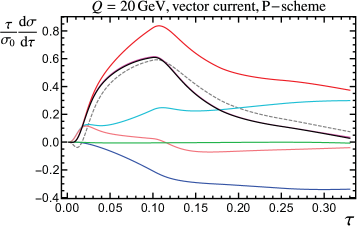
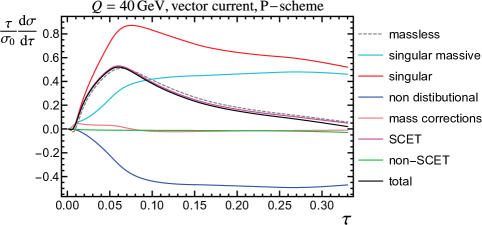
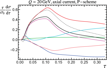
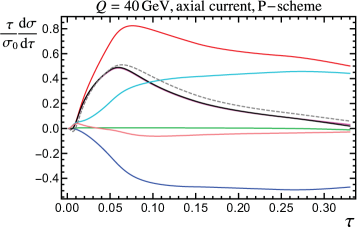
Figure 7: Decomposition of the differential cross section at $Q=20\,$GeV (left panels) and $40\,$GeV (right panels) in various components for the vector (upper plots) and axial-vector (lower plots) currents. Red and blue correspond to the singular and non-distributional terms, respectively, while their sum defines the SCET cross section, shown in magenta. The massless approximation is shown as a dashed gray line, while massive singular corrections are depicted in cyan. The massive corrections to the SCET cross section (massive singular plus non-distributional) are shown in pink. Finally, the black solid line is the sum of all contributions.

We start our numerical discussion by analyzing the size of each term in Fig. 7, which shows differential cross sections for $Q=20\,$GeV and $40\,$GeV for vector and axial-vector currents. We use only the default parameters for the profiles and set the parameter $\xi$ defined in Eq. (138) to its canonical value $0.5$. We split the distribution as follows (to alleviate notation, in the remainder of this section we drop the superscript $C$ that indicates the current):

$$\frac{\mathrm{d}\sigma}{\mathrm{d}\tau}=\, \frac{\mathrm{d}\sigma_{\rm SCET}}{\mathrm{d}\tau}+\frac{\mathrm{d}\sigma_{\rm NS}}{\mathrm{d}\tau}\equiv\frac{\mathrm{d}\sigma_{\rm sing}}{\mathrm{d}\tau}+\frac{\mathrm{d}\sigma_{\rm nd}}{\mathrm{d}\tau}+\frac{\mathrm{d}\sigma_{\rm NS}}{\mathrm{d}\tau}$$ (142)

$$\equiv\, \frac{\mathrm{d}\sigma^{\rm sing}_{m=0}}{\mathrm{d}\tau}+\frac{\mathrm{d}\sigma^{\rm sing}_{m}}{\mathrm{d}\tau}+\frac{\mathrm{d}\sigma_{\rm nd}}{\mathrm{d}\tau}+\frac{\mathrm{d}\sigma_{\rm NS}}{\mathrm{d}\tau}\equiv\frac{\mathrm{d}\sigma^{\rm sing}_{m=0}}{\mathrm{d}\tau}+\frac{\mathrm{d}\sigma^{\rm SCET}_{m}}{\mathrm{d}\tau}+\frac{\mathrm{d}\sigma_{\rm NS}}{\mathrm{d}\tau}\,,$$

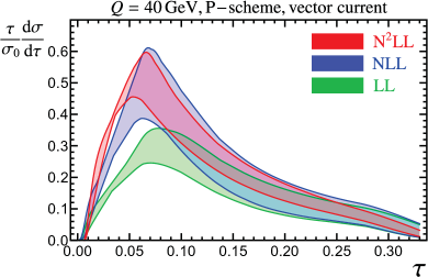
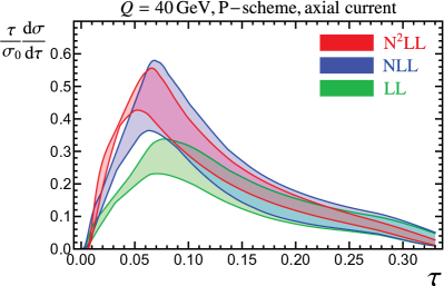
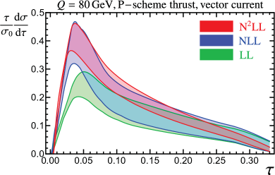
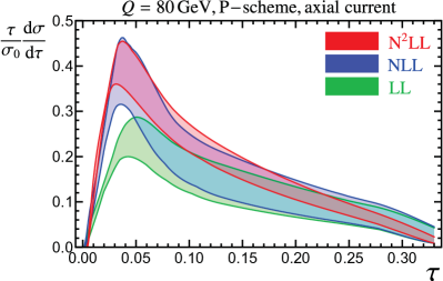
Figure 8: Uncertainty bands for LL (green), NLL (blue) and N²LL (red) for P-scheme thrust cross sections at $40$ GeV (figures on top) and $80\,$GeV (figures at the bottom), for vector (left figures) and axial-vector (right figures) currents. The bands are obtained with $500$ profiles generated randomly selecting values for the parameters that define them.

​where each term contains hadronization power corrections computed as a convolution with the same shape function. In the first equality we split the full cross section (shown as a black solid line) in SCET and non-SCET contributions, shown in magenta and green, respectively. The SCET cross section can be further divided into the sum of singular $\mathrm{d}\sigma^{\rm sing}_{m}/\mathrm{d}\tau$ (shown as a red solid line) and non-distributional $\mathrm{d}\sigma_{\rm nd}/\mathrm{d}\tau$ (in solid blue) contributions. In our setup, the singular cross section is defined as the contribution from terms in the SCET factorization theorem which are singular at threshold if no resummation is implemented. At N²LL, these correspond to the distributions that arise from the hard function, the 1-loop soft function, and the $J_{m=0}$, $J_{m}$ pieces of the one-loop jet function, with the modifications discussed in Sec. 9 to absorb the relevant mass corrections, integrated against the resummation kernels. The non-distributional terms (shown in blue) are defined as the resummed contribution from $J_{\rm nd}$ defined in Eq. (4.1). We observe that while the singular contribution is positive, the non-distributional is negative, and they significantly cancel each other when added together. The singular distribution can be cast as the sum of the massless approximation $\mathrm{d}\sigma^{\rm sing}_{m=0}/\mathrm{d}\tau$ (shown as a dashed gray line) and singular massive corrections $\mathrm{d}\sigma^{\rm sing}_{m}/\mathrm{d}\tau$ (cyan solid line). The massless approximation is quite close to the SCET cross section (specially for the vector current), as expected, since the P-scheme decreases the sensitivity to the quark mass, and the singular massive corrections are very similar to the non-distributional term up to a global sign. We define the SCET massive corrections $\mathrm{d}\sigma^{\rm SCET}_{m}/\mathrm{d}\tau$ (pink solid line) as the sum of the singular massive corrections and the non-distributional terms, which turns out to be rather small, specially for larger values of the center-of-mass energy. The non-SCET cross section has been defined in Eq. (139) and contains non-distributional kinematic corrections coming from the QCD fixed-order cross section. Interestingly, once we absorb all singular terms into the SCET factorization theorem, the non-SCET corrections are absolutely negligible everywhere except in the far tail. Within the setup defined in Sec. 9 only the non-distributional cross section and the massless approximation is the same for vector and axial-vector currents.

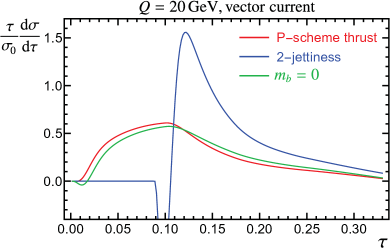
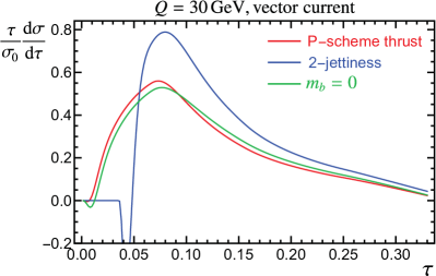
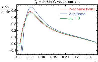
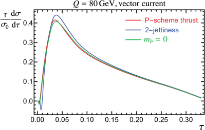
Figure 9: Differential cross section for massless quarks (green lines), 2-jettiness (blue lines) and P-scheme thrust (red lines) produced through the vector current. Panels (a), (b), (c) and (d) correspond to center-of-mass energies of $20$, $30$, $50$ and $80\,$GeV, respectively.

We study next the convergence of the (resummed) perturbative series for the differential cross section. To that end, we generate bands randomly modifying our profile functions via a flat scan on their parameters, varying them within the ranges specified in Ref. Hoang:2014wka , with the exception of the non-singular scale, for which we use the following continuous variation

$$\mu_{\rm ns}=\frac{1}{2}[(2+ns)\mu_{H}-\mu_{J}]\,,$$ (143)

with $-1\leq n_{s}\leq 1$. In our scan we also randomly vary $\xi$ between $0$ and $1$. In Fig. 8 we show the resulting perturbative bands at LL (green), NLL (blue) and N²LL + $\mathcal{O}(\alpha_{s})$ (red) for the vector and axial-vector currents, at two center-of-mass energies: $Q=40\,$GeV and $80\,$GeV. Our curves are not self-normalized, but we nevertheless observe an excellent convergence in all cases (even at low energies) in the tail of the distribution, where higher-order bands are nicely contained in lower-order ones. In the peak we see a big jump between LL and the two highest orders, and the convergence is not as good as in the tail, what might indicate that the parameters affecting mainly the peak should be varied in wider ranges. A careful inspection of the error bands reveals that the relative uncertainties for LL and NLL are nearly identical in the whole range, and both monotonically increase as $\tau$ grows: at $Q=40\,[80]\,$GeV they change from $36\,[45]\%$ at $\tau=0.07$ to $84\,[80]\%$ at $\tau=0.28$. On the other hand, at N²LL the relative uncertainty is completely flat between $0.07\leq\tau\leq 0.3$, and smaller than the two lower orders: $36\,[30]\%$ for $Q=40\,[80]\,$GeV. We observe the same relative uncertainties for vector and axial-vector currents.

In Fig. 9 we compare the 2-jettiness (blue) and thrust (red) cross sections for massive quarks produced through the vector current at various center of mass energies, as indicated in the caption of the plot. As a reference, we also show in green the massless cross section. We observe that the 2-jettiness cross section has a negative deep which becomes more pronounced at low energies. It is produced by large logarithms which could be summed up by matching SCET to bHQET, as discussed in Sec. 4.2. While the massless cross section is always quite similar to massive P-scheme thrust, the 2-jettiness distribution gets quite different at low energies, with a higher peak shifted to the right. We will study this behavior in further detail later in this section. As energies become larger, the three cross sections become similar to one another, but P-scheme thrust is always closer to the massless result. In Fig. 10 we plot the difference between the vector and axial-vector currents normalized to their average. To make the figure clearer, we use a logarithmic scale on the $y$ axis. We observe, as expected, that for larger energies the difference becomes smaller, since both currents approach the (current-independent) massless result.

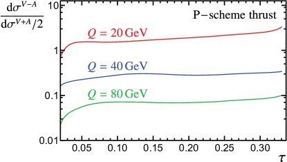
Figure 10: Difference between the vector and axial-vector differential cross sections normalized to the average of the two currents. We show results for $Q=20\,$GeV (red), $Q=40\,$GeV (blue) and $Q=80\,$GeV (green).

In our last analysis we study the dependence of the peak position and peak height with the heavy quark mass. Since the peak position retains some dependence on $Q$ from soft hadronization, we fix the value of the center-of-mass energy to $40\,$GeV, such that we can make sure the peak moves only due to changes in the mass. In this case we compare the results for thrust and 2-jettiness, since the former is relatively mass insensitive while the latter has been designed to measure the top quark mass in future linear colliders, see e.g. Ref. Fleming:2007qr . We restrict the values of the bottom quark below $m_{b}=14\,$GeV to make sure we can still apply SCET and scenario II, which should be described using bHQET, is unimportant. The results of our study are summarized in Fig. 11, where one can clearly observe a flat behavior for P-scheme and an obvious quadratic dependence for 2-jettiness. The latter is nothing but expected, since the peak position is shifted by $\tau^{J}_{\min}=1-\sqrt{1-4\hat{m}^{2}}\simeq 2\hat{m}^{2}$. In fact, if we perform a fit to the 2-jettiness peak position we find $\tau_{\rm max}\simeq 0.0255+1.75\hat{m}^{2}$, which follows almost exactly the blue line in Fig. 11 and is in fair agreement with our expectations [ the small disagreement is expected since the peak position should be computed with $\overline{m}_{b}(\mu_{J})$ and not with $\overline{m}_{b}(\overline{m}_{b})$ ]. The dependence of the peak height on the bottom mass is also much larger in jettiness than P-scheme thrust.

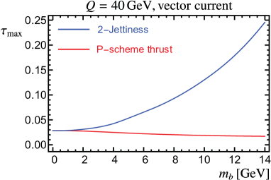
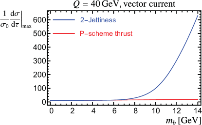
Figure 11: Peak position (a) and peak height (b) for 2-jettiness (blue) and P-scheme thrust (red) massive cross section. Results correspond to default profiles, vector current and a center-of-mass energy of $40\,$GeV, and with $m_{b}\equiv\overline{m}_{b}(\overline{m}_{b})$. We vary the bottom mass between $0$ and $14\,$GeV, such that SCET still applies.

11 Conclusions

When considering heavy quarks in the context of event shapes, depending on the scheme used in their definition the mass sensitivity of the cross section can vary significantly. This sensitivity manifests itself already at lowest order by setting the threshold position to a non-zero value, and of course increases as the mass grows. This shifted threshold comes solely from the jet function.

While in a recent paper we discussed how to obtain these distributions in fixed-order at NLO, in this article we have shown how to analytically compute the differential and cumulative cross sections in the E- and P-schemes at N²LL + $\mathcal{O}(\alpha_{s})$ accuracy in SCET and bHQET. To achieve this goal, we have calculated the missing pieces, namely the NLO jet function in those two effective field theories. We have shown that in the collinear limit the heavy quark momenta expressed in the E- and P-schemes coincide, but are different from the original (massive) definition. This entails that for any event shape, the jet function will be identical in the former two schemes, but in the case of thrust, heavy jet mass and C-parameter the measurement function is no longer completely inclusive, meaning that one needs to compute the jet function with cut diagrams, integrating over phase space rather than loop momenta. We provide an optimized and compact form for the jet function definition in each EFT, written in terms of quantum and kinematic operators, that facilitates their computation. For the bHQET jet function we explain how to rescale the integrated light-particle momenta such that the heavy quark mass drops out before any integration is carried out. In the computation of the P-scheme SCET jet function one needs to use either sector decomposition or hypergeometric function identities to properly expand in $\varepsilon$ and extract the distributions that appear in this limit.

Shifting its argument to relocate the threshold back to zero, the 1-loop SCET massive jet functions can be written as the sum of the massless jet function plus mass corrections. The latter can be further divided into terms with distributions (or singular) and terms without distributions. While carrying out resummation for the former is already well known, the terms with regular functions need to be treated in a case-by-case basis. In this article we show how to analytically RG evolve the non-distributional terms for 2-jettiness and P-scheme thrust, and derive rapidly-convergent expansions that can be carried out around the threshold ($\tau-\tau_{\rm min}=0$), “singular” ($Q^{2}\tau=m^{2}$) [ only for P- and E-schemes ] and massless ($Q^{2}\tau\gg m^{2}$) limits, which nicely overlap with one another such that in numerical implementations there is no need to explicitly evaluate hypergeometric functions at all (for 2-jettiness there is a small region around $Q^{2}\tau=m^{2}$ for which one cannot use expansions). Our expansions can be carried out up to any order such that the result is also arbitrarily precise. This is much faster than a direct evaluation of ${}_{2}F_{1}$ and ${}_{3}F_{2}$ functions, which were the bottleneck of the analysis carried out in Ref. Butenschoen:2016lpz .

We show how to absorb into the SCET factorization theorem those mass-suppressed singular terms that appear in fixed-order corrections by a suitable redefinition of the hard and jet functions. After this procedure is carried out, we complete our resummed expression with purely kinematic corrections (which are now entirely non-singular), which become relevant in the far tail. Hadronization power corrections can be incorporated in the usual way by convolving with a shape function, and with this complete description we have performed some numerical investigations. We have shown that there are strong cancellations taking place between the two types of mass corrections to the SCET factorization theorem (with or without distributions) everywhere except in the peak, and that the remaining non-singular corrections are immaterial everywhere except in the far tail. The cancellations are stronger at larger energies, where also vector and axial-vector currents yield similar results. We have demonstrated that the P-scheme thrust cross section is much closer to the massless prediction than for 2-jettiness by comparing cross sections as well as investigating the peak position and height as a function of the heavy quark mass. We have also observed a nice convergence of the cross section when adding perturbative orders.

These results will be highly important for ongoing and forthcoming research in the field of event shapes with massive quarks. They will play a relevant role in the determination of $\alpha_{s}$ with high precision (when the bottom quark mass cannot be neglected any longer) and in the Monte Carlo top quark mass parameter calibration. In addition, the computations we have carried out will be very valuable for top quark mass measurement carried out at future linear colliders. Our computations can be applied to other relevant event-shapes such as angularities, groomed observables like Soft Drop Larkoski:2014wba or even recoil-sensitive observables like jet-broadening. These will be presented in forthcoming publications. Extending our computations to $\mathcal{O}(\alpha_{s}^{2})$ is certainly challenging, but at least for the bHQET jet function, calculations of similar complexity have been carried out for the soft function e.g. in Refs. Hornig:2011iu ; Kelley:2011ng ; Monni:2011gb ; vonManteuffel:2013vja , and even numerical approaches have been devised in Refs. Bell:2018vaa ; Bell:2018oqa . The massive SCET jet function at $\mathcal{O}(\alpha_{s}^{2})$ is definitely much more involved, and so far results only exist for 2-jettiness Hoang:2019fze , which is certainly simpler since it can be computed as the imaginary part of a forward-scattering matrix element, such that the usual machinery for multi-loop computations can be applied.

Appendix A Sector Decomposition

The direct $\varepsilon$ expansion of $J_{a,P}^{\rm real}$ becomes much simpler if one does not have to deal with distributions, therefore we consider the cumulative jet function, and to that end we define

$$\Sigma_{a}(s_{c},\mu)\equiv\!\int_{0}^{s_{c}}\!{\rm d}s\,J^{\rm real}_{a,P}(s,\mu)\,.$$ (144)

Switching variables to $s=ys_{c}$ in Eq. (144) and $x\to 1-x$ in Eq. (53) we get

$$\Sigma_{a}(s_{c},\mu)=\, \frac{C_{F}\alpha_{s}}{2\pi\Gamma(1-\varepsilon)}\biggl{(}\frac{s_{c}}{\mu^{2}}\biggr{)}^{\!\!-\varepsilon}I_{3}\biggl{(}\frac{m^{2}}{s_{c}}\biggr{)}\,,$$ (145)

$$I_{3}(t)\equiv\, \int_{0}^{1}\!{\rm d}y\,y^{-\varepsilon}\!\!\int_{0}^{1}\!\!{\rm d}x\,\frac{(1-x)^{2-\varepsilon}x^{-1-\varepsilon}}{y(1-x)+t\,x}\,.$$

We apply sector decomposition by splitting the $x$ integration in two segments: $(0,y)$ and $(y,1)$. In the former we switch variables to $x=zy$ and in the latter we reverse the order of integration, which is followed by the change of variables $y=z\,x$, to find

$$I_{3}(t)= \!\int_{0}^{1}\!\!{\rm d}y\,y^{-1-2\varepsilon}\!\!\int_{0}^{1}\!\!{\rm d}z\,\frac{(1-zy)^{2-\varepsilon}z^{-1-\varepsilon}}{(1-zy)+t\,z}+\!\!\int_{0}^{1}\!{\rm d}x\,x^{-1-2\varepsilon}(1-x)^{2-\varepsilon}\!\!\int_{0}^{1}\!\!\frac{{\rm d}z\,z^{-\varepsilon}}{(1-x)z+t}$$

$$\equiv \;I_{3}^{\alpha}(t)+I_{3}^{\beta}(t)\,.$$ (146)

Since the original singularities at $x=0,1$ have been properly separated, mapping the former at $y=0$ and the latter at $x=0$, one can expand in $\varepsilon$ before integrating. Let us solve $I_{3}^{\beta}$ first, which has a single pole only, such that we can use Eq. (55) on $x^{-1-2\varepsilon}$ to obtain

$$I_{3}^{\beta}(t)= -\!\frac{1}{2\varepsilon}\!\int_{0}^{1}\!\!\frac{{\rm d}z}{z+t}\bigl{[}1-\varepsilon\log(z)\bigr{]}+\!\!\int_{0}^{1}{\rm d}x\int_{0}^{1}{\rm d}z\,\frac{2t-tx-xz+z}{(t+z)(xz-t-z)}$$ (147)

$$= -\!\frac{1}{2\varepsilon}\log\biggl{(}1+\frac{1}{t}\biggr{)}+\frac{1}{2}\text{Li}_{2}\biggl{(}-\frac{1}{t}\biggr{)}-(1+t)\log\biggl{(}1+\frac{1}{t}\biggr{)}-\text{Li}_{2}\biggl{(}\frac{1}{1+t}\biggr{)}+1\,.$$

For $I_{3}^{\alpha}$ one must start applying Eq. (55) to $y^{-1-2\varepsilon}$ in order to regulate the pole of the $z$-integral. Taking into account the plus-function prescription and that the upper integration limit is $1$ we get

$$I_{3}^{\alpha}(t)=-\frac{1}{2\varepsilon}\!\int_{0}^{1}\!{\rm d}z\,\frac{z^{-1-\varepsilon}}{1+t\,z}-\!\int_{0}^{1}{\rm d}y\!\int_{0}^{1}\!{\rm d}z\,\frac{1+tz(2-yz)-yz}{(1+tz)(1+tz-yz)}\,,$$ (148)

where in the second term we have already set $\varepsilon=0$. Using again Eq. (55) to expand $z^{-1-\varepsilon}$ in $\varepsilon$ and solving the resulting integrals we arrive at

$$I_{3}^{\alpha}(t)= \,\frac{1}{2\varepsilon^{2}}+\frac{1}{2\varepsilon}\log(1+t)+\frac{1}{2}\,\text{Li}_{2}(-t)-\text{Li}_{2}(1-t)+\text{Li}_{2}\Bigl{(}\frac{1}{1+t}\Bigr{)}$$ (149)

$$-\frac{t}{t-1}\log(t)+t\log(1+t)+\log(1+t)-1\,.$$

Thus, summing $I_{3}^{\alpha}$ and $I_{3}^{\beta}$ we obtain:

$$I_{3}(t)=\,\frac{1}{2\varepsilon^{2}}+\frac{1}{2\varepsilon}\log(t)+\text{Li}_{2}\Bigl{(}\frac{1}{1-t}\Bigr{)}+\frac{1}{2}\log^{2}(t-1)-\frac{1}{4}\log^{2}(t)-\frac{1}{t-1}\log(t)+\frac{\pi^{2}}{12}\,.$$ (150)

To obtain this expression, which facilitates taking the $t\to\infty$ limit (that corresponds to $s_{c}\to 0$), we have applied the following identities of dilogarithms:

$$\text{Li}_{2}(z)= -\!\text{Li}_{2}(1-z)-\log(1-z)\log(z)+\frac{\pi^{2}}{6}\,,$$ (151)

$$\text{Li}_{2}(z)= -\!\text{Li}_{2}\Bigl{(}\frac{1}{z}\Bigr{)}-\frac{1}{2}\log^{2}(-z)-\frac{\pi^{2}}{6}\,,$$

where the second line holds for $z\notin(0,1)$ only. Now we insert Eq. (150) into (145) and expanding again in $\varepsilon$ becomes trivial. To compute $J_{a,P}^{\rm real}$ we have to take the derivative of $\Sigma_{a}(s_{c})$ with respect to $s_{c}$ taking into account that it has support only for $s_{c}>0$:

$$J_{a,P}^{\rm real}(s,\mu)=\frac{\text{d}}{\text{d}s}\Bigl{[}\theta(s)\,\Sigma_{a}(s,\mu)\Bigr{]}.$$ (152)

Using the relations in Eq. (79)  and the identity given in Eq. (3.6) of Ref. Lepenik:2019jjk one arrives at the result quoted in Eq. (5.2.1).

Appendix B Alternative Analytic Expression of $I^{P}_{\rm nd}$ for $s>m^{2}$

In this appendix we present an alternative form of $I^{P}_{\rm nd}$ in which all terms are manifestly real for $y>1$ and where no numerical derivatives are involved. In a first step we express ${}_{2}F_{1}(1,1+\varepsilon,2+\tilde{\omega},1-y)$ in Eq. (8) in terms ${}_{2}F_{1}(1,1+\varepsilon,1-\tilde{\omega}+\varepsilon,y)$ through Eq. (110), and then use that for $y>1$ one has 

$${}_{2}F_{1}(1,1+\varepsilon,1-\tilde{\omega}+\varepsilon,y)=\, \!-\!\frac{\tilde{\omega}\,\pi(y-1)^{-1-\tilde{\omega}}\left[\cot(\pi\varepsilon)+i\,\right]y^{\tilde{\omega}-\varepsilon}\,\Gamma(1-\tilde{\omega}+\varepsilon)}{\Gamma(1-\tilde{\omega})\Gamma(\varepsilon+1)}$$ (155)

$$\!+\!\frac{(\tilde{\omega}-\varepsilon)}{y\varepsilon}\,{}_{2}F_{1}\!\biggl{(}1,1+\tilde{\omega}-\varepsilon,1-\varepsilon,\frac{1}{y}\biggr{)}.$$

The only involved computation left is finding an analytic expression for the derivative of ${}_{2}F_{1}(1,1+\tilde{\omega}-\varepsilon,1-\varepsilon,1/y)$ with respect to $\varepsilon$ in the $\varepsilon\rightarrow 0$ limit. The complication here arises because there are poles in $1/\varepsilon$ such that one also needs the second derivative, which as we shall see implies the appearance of the ${}_{4}F_{3}$ function. A practical way of doing the derivative is by Taylor expanding. The first derivative reads

$$\frac{{\rm d}}{{\rm d}\varepsilon}{}_{2}F_{1}(1,1+\tilde{\omega}-\varepsilon,1-\varepsilon,y)=\frac{y\,\tilde{\omega}(1-y)^{-1-\tilde{\omega}}}{(1-\varepsilon)^{2}}\,{}_{3}F_{2}(1-\tilde{\omega},1-\varepsilon,1-\varepsilon,2-\varepsilon,2-\varepsilon,y)\,.$$ (156)

For the second one needs the first derivative of the ${}_{3}F_{2}$ function:

$$\frac{{\rm d}}{{\rm d}\varepsilon}\,{}_{3}F_{2}(1-\tilde{\omega},1-\varepsilon,1-\varepsilon,2-\varepsilon,2-\varepsilon,y)=$$ (157)

$$\qquad-\!\frac{2y(1-\tilde{\omega})(1-\varepsilon)}{(2-\varepsilon)^{3}}\,{}_{4}F_{3}(2-\tilde{\omega},2-\varepsilon,2-\varepsilon,2-\varepsilon,3-\varepsilon,3-\varepsilon,3-\varepsilon,y)\,.$$

With these results one can obtain the Taylor expansion of ${}_{2}F_{1}(1,1+\tilde{\omega}-\varepsilon,1-\varepsilon,1/y)$, which allows to compute the first derivative of ${}_{2}F_{1}(1,1+\varepsilon,1-\tilde{\omega}+\varepsilon,y)$

$$\frac{\rm d}{{\rm d}\varepsilon}{}_{2}F_{1}(1,1+\varepsilon,1-\tilde{\omega}+\varepsilon,y)\Bigr{|}_{\varepsilon\rightarrow 0}$$ (158)

$$=\, \frac{\tilde{\omega}(y-1)^{-\tilde{\omega}-1}y^{\tilde{\omega}-1}}{12}\biggl{\{}12\,\tilde{\omega}\,{}_{4}F_{3}\!\biggl{(}1,1,1,1-\tilde{\omega},2,2,2,\frac{1}{y}\biggr{)}-12\,{}_{3}F_{2}\!\biggl{(}1,1,1-\tilde{\omega},2,2,\frac{1}{y}\biggr{)}$$

$$y\Big{[}6(H_{-\tilde{\omega}}-\log(y))(2i\pi-H_{-\tilde{\omega}}+\log(y))-6\psi^{(1)}(1-\tilde{\omega})+5\pi^{2}\Big{]}\biggr{\}}.$$

Using this result we arrive at the alternative expression for $I^{P}_{\rm nd}$

$$I^{P}_{\rm nd}(\tilde{\omega},y)=\frac{\tilde{\omega}[(2\tilde{\omega}+5)y+\tilde{\omega}(3\tilde{\omega}+7)-4y^{2}]}{\Gamma(1-\tilde{\omega})(1+\tilde{\omega})(1-y)^{2}}\biggl{[}H_{1-\tilde{\omega}}-\frac{1}{1-\tilde{\omega}}-\log(y)\biggr{]}{}_{2}F_{1}(1,1,\tilde{\omega}+2,1-y)$$

$$+\frac{3\tilde{\omega}^{2}y+3\tilde{\omega}^{2}-5\tilde{\omega}y+14\tilde{\omega}+y-7}{\Gamma(2-\tilde{\omega})(y-1)^{2}}+(y-1)^{-3-\tilde{\omega}}y^{\tilde{\omega}-1}[4y^{2}-2(\tilde{\omega}+5)y-\tilde{\omega}(3\tilde{\omega}+7)]$$

$$\times\biggl{\{}\tilde{\omega}^{2}{}_{4}F_{3}\!\biggl{(}1,1,1,1-\tilde{\omega},2,2,2,\frac{1}{y}\biggr{)}-\tilde{\omega}\,_{3}F_{2}\!\biggl{(}1,1,1-\tilde{\omega},2,2,\frac{1}{y}\biggr{)}$$ (159)

$$\times\frac{\tilde{\omega}\,y}{12}\biggl{[}5\pi^{2}-6\biggl{(}\!H_{1-\tilde{\omega}}-\frac{1}{1-\tilde{\omega}}-\log(y)\!\biggr{)}^{\!\!2}-6\psi^{(1)}(1-\tilde{\omega})\biggr{]}$$

$$+y\cos(\pi\tilde{\omega})\Gamma(1-\tilde{\omega})\Gamma(1+\tilde{\omega})_{2}F_{1}(1,1,2+\tilde{\omega},1-y)\!\biggl{[}H_{1-\tilde{\omega}}-\frac{1}{1-\tilde{\omega}}-\log(y)\biggr{]}\!\biggr{\}}.$$

References

- (1) M. Dasgupta and G. P. Salam, Event shapes in annihilation and deep inelastic scattering, J.Phys. G30 (2004) R143, [hep-ph/0312283].
- (2) S. Kluth, Tests of quantum chromo dynamics at colliders, Rept. Prog. Phys. 69 (2006) 1771–1846, [hep-ex/0603011].
- (3) A. Gehrmann-De Ridder, T. Gehrmann, E. W. N. Glover and G. Heinrich, Second-order QCD corrections to the thrust distribution, Phys. Rev. Lett. 99 (2007) 132002, [0707.1285].
- (4) A. Gehrmann-De Ridder, T. Gehrmann, E. W. N. Glover and G. Heinrich, NNLO corrections to event shapes in annihilation, JHEP 12 (2007) 094, [0711.4711].
- (5) S. Weinzierl, NNLO corrections to 3-jet observables in electron-positron annihilation, Phys. Rev. Lett. 101 (2008) 162001, [0807.3241].
- (6) A. Gehrmann-De Ridder, T. Gehrmann, E. Glover and G. Heinrich, EERAD3: Event shapes and jet rates in electron-positron annihilation at order , Comput. Phys. Commun. (2014) , [1402.4140].
- (7) S. Weinzierl, Event shapes and jet rates in electron-positron annihilation at NNLO, JHEP 06 (2009) 041, [0904.1077].
- (8) V. Del Duca, C. Duhr, A. Kardos, G. Somogyi, Z. Szőr, Z. Trócsányi et al., Jet production in the CoLoRFulNNLO method: event shapes in electron-positron collisions, Phys. Rev. D94 (2016) 074019, [1606.03453].
- (9) A. Hornig, C. Lee and G. Ovanesyan, Effective Predictions of Event Shapes: Factorized, Resummed, and Gapped Angularity Distributions, JHEP 05 (2009) 122, [0901.3780].
- (10) T. Becher and G. Bell, NNLL Resummation for Jet Broadening, JHEP 1211 (2012) 126, [1210.0580].
- (11) G. Bell, A. Hornig, C. Lee and J. Talbert, angularity distributions at NNLL′ accuracy, JHEP 01 (2019) 147, [1808.07867].
- (12) T. Becher and M. D. Schwartz, A Precise determination of from LEP thrust data using effective field theory, JHEP 07 (2008) 034, [0803.0342].
- (13) Y.-T. Chien and M. D. Schwartz, Resummation of heavy jet mass and comparison to LEP data, JHEP 08 (2010) 058, [1005.1644].
- (14) A. H. Hoang, D. W. Kolodrubetz, V. Mateu and I. W. Stewart, -parameter distribution at N3LL′ including power corrections, Phys. Rev. D91 (2015) 094017, [1411.6633].
- (15) I. Moult and H. X. Zhu, Simplicity from Recoil: The Three-Loop Soft Function and Factorization for the Energy-Energy Correlation, JHEP 08 (2018) 160, [1801.02627].
- (16) A. H. Hoang, V. Mateu, M. Schwartz and I. W. Stewart, Precision Hemisphere Masses with Power Corrections, Work in progress (2020) .
- (17) C. W. Bauer, S. Fleming and M. E. Luke, Summing Sudakov logarithms in in effective field theory, Phys. Rev. D63 (2000) 014006, [hep-ph/0005275].
- (18) C. W. Bauer, S. Fleming, D. Pirjol and I. W. Stewart, An Effective field theory for collinear and soft gluons: Heavy to light decays, Phys. Rev. D63 (2001) 114020, [hep-ph/0011336].
- (19) C. W. Bauer and I. W. Stewart, Invariant operators in collinear effective theory, Phys. Lett. B516 (2001) 134–142, [hep-ph/0107001].
- (20) C. W. Bauer, D. Pirjol and I. W. Stewart, Soft-Collinear Factorization in Effective Field Theory, Phys. Rev. D65 (2002) 054022, [hep-ph/0109045].
- (21) C. W. Bauer, S. Fleming, D. Pirjol, I. Z. Rothstein and I. W. Stewart, Hard scattering factorization from effective field theory, Phys. Rev. D66 (2002) 014017, [hep-ph/0202088].
- (22) J. C. Collins and D. E. Soper, Back-To-Back Jets in QCD, Nucl. Phys. B193 (1981) 381.
- (23) G. P. Korchemsky, Shape functions and power corrections to the event shapes, hep-ph/9806537.
- (24) G. P. Korchemsky and G. Sterman, Power corrections to event shapes and factorization, Nucl. Phys. B555 (1999) 335–351, [hep-ph/9902341].
- (25) G. P. Korchemsky and S. Tafat, On power corrections to the event shape distributions in QCD, JHEP 10 (2000) 010, [hep-ph/0007005].
- (26) C. F. Berger, T. Kúcs and G. Sterman, Event shape / energy flow correlations, Phys. Rev. D68 (2003) 014012, [hep-ph/0303051].
- (27) S. Catani, L. Trentadue, G. Turnock and B. R. Webber, Resummation of large logarithms in event shape distributions, Nucl. Phys. B407 (1993) 3–42.
- (28) A. Banfi, G. P. Salam and G. Zanderighi, Principles of general final-state resummation and automated implementation, JHEP 03 (2005) 073, [hep-ph/0407286].
- (29) A. Banfi, H. McAslan, P. F. Monni and G. Zanderighi, A general method for the resummation of event-shape distributions in annihilation, JHEP 05 (2015) 102, [1412.2126].
- (30) V. Mateu and G. Rodrigo, Oriented Event Shapes at N3LL, JHEP 1311 (2013) 030, [1307.3513].
- (31) R. Abbate, M. Fickinger, A. H. Hoang, V. Mateu and I. W. Stewart, Thrust at N3LL with Power Corrections and a Precision Global Fit for , Phys. Rev. D83 (2011) 074021, [1006.3080].
- (32) R. Abbate, M. Fickinger, A. H. Hoang, V. Mateu and I. W. Stewart, Precision Thrust Cumulant Moments at N3LL, Phys. Rev. D86 (2012) 094002, [1204.5746].
- (33) T. Gehrmann, G. Luisoni and P. F. Monni, Power corrections in the dispersive model for a determination of the strong coupling constant from the thrust distribution, Eur. Phys. J. C73 (2013) 2265, [1210.6945].
- (34) A. H. Hoang, D. W. Kolodrubetz, V. Mateu and I. W. Stewart, Precise determination of from the -parameter distribution, Phys. Rev. D91 (2015) 094018, [1501.04111].
- (35) A. H. Hoang, V. Mateu, M. Schwartz and I. W. Stewart, A Precise Determination of from the Heavy Jet Mass Distribution, Work in progress (2020) .
- (36) C. Lepenik and V. Mateu, NLO Massive Event-Shape Differential and Cumulative Distributions, JHEP 03 (2020) 024, [1912.08211].
- (37) S. Fleming, A. H. Hoang, S. Mantry and I. W. Stewart, Jets from massive unstable particles: Top-mass determination, Phys. Rev. D77 (2008) 074010, [hep-ph/0703207].
- (38) S. Fleming, A. H. Hoang, S. Mantry and I. W. Stewart, Top Jets in the Peak Region: Factorization Analysis with NLL Resummation, Phys. Rev. D77 (2008) 114003, [0711.2079].
- (39) A. K. Leibovich, Z. Ligeti and M. B. Wise, Comment on quark masses in SCET, Phys. Lett. B 564 (2003) 231–234, [hep-ph/0303099].
- (40) A. Jain, I. Scimemi and I. W. Stewart, Two-loop Jet-Function and Jet-Mass for Top Quarks, Phys. Rev. D77 (2008) 094008, [0801.0743].
- (41) A. H. Hoang, C. Lepenik and M. Stahlhofen, Two-Loop Massive Quark Jet Functions in SCET, JHEP 08 (2019) 112, [1904.12839].
- (42) A. H. Hoang, A. Pathak, P. Pietrulewicz and I. W. Stewart, Hard Matching for Boosted Tops at Two Loops, JHEP 12 (2015) 059, [1508.04137].
- (43) S. Gritschacher, A. H. Hoang, I. Jemos and P. Pietrulewicz, Secondary Heavy Quark Production in Jets through Mass Modes, Phys. Rev. D88 (2013) 034021, [1302.4743].
- (44) P. Pietrulewicz, S. Gritschacher, A. H. Hoang, I. Jemos and V. Mateu, Variable Flavor Number Scheme for Final State Jets in Thrust, Phys.Rev. D90 (2014) 114001, [1405.4860].
- (45) M. Butenschoen, B. Dehnadi, A. H. Hoang, V. Mateu, M. Preisser and I. W. Stewart, Top Quark Mass Calibration for Monte Carlo Event Generators, Phys. Rev. Lett. 117 (2016) 232001, [1608.01318].
- (46) C. W. Bauer, S. P. Fleming, C. Lee and G. F. Sterman, Factorization of Event Shape Distributions with Hadronic Final States in Soft Collinear Effective Theory, Phys. Rev. D78 (2008) 034027, [0801.4569].
- (47) V. Mateu, I. W. Stewart and J. Thaler, Power Corrections to Event Shapes with Mass-Dependent Operators, Phys. Rev. D87 (2013) 014025, [1209.3781].
- (48) G. P. Salam and D. Wicke, Hadron masses and power corrections to event shapes, JHEP 05 (2001) 061, [hep-ph/0102343].
- (49) C. F. Berger and G. Sterman, Scaling rule for nonperturbative radiation in a class of event shapes, JHEP 09 (2003) 058, [hep-ph/0307394].
- (50) E. Farhi, A QCD Test for Jets, Phys. Rev. Lett. 39 (1977) 1587–1588.
- (51) G. Parisi, Super Inclusive Cross-Sections, Phys. Lett. B74 (1978) 65.
- (52) J. F. Donoghue, F. Low and S.-Y. Pi, Tensor Analysis of Hadronic Jets in Quantum Chromodynamics, Phys. Rev. D20 (1979) 2759.
- (53) P. E. Rakow and B. Webber, Transverse Momentum Moments of Hadron Distributions in QCD Jets, Nucl.Phys. B191 (1981) 63.
- (54) L. Clavelli, Jet Invariant Mass in Quantum Chromodynamics, Phys.Lett. B85 (1979) 111.
- (55) T. Chandramohan and L. Clavelli, Consequences of Second Order QCD for Jet Structure in annihilation, Nucl.Phys. B184 (1981) 365.
- (56) L. Clavelli and D. Wyler, Kinematica Bounds on Jet Variables and the Heavy Jet Mass Distribution, Phys.Lett. B103 (1981) 383.
- (57) I. W. Stewart, F. J. Tackmann and W. J. Waalewijn, Factorization at the LHC: From PDFs to Initial State Jets, Phys.Rev. D81 (2010) 094035, [0910.0467].
- (58) E. Gardi and L. Magnea, The C parameter distribution in annihilation, JHEP 0308 (2003) 030, [hep-ph/0306094].
- (59) M. Preisser, C-Parameter with massive quarks, Master’s thesis, Vienna U., 2014.
- (60) A. H. Hoang, A. Jain, I. Scimemi and I. W. Stewart, Infrared Renormalization Group Flow for Heavy Quark Masses, Phys. Rev. Lett. 101 (2008) 151602, [0803.4214].
- (61) A. H. Hoang, A. Jain, C. Lepenik, V. Mateu, M. Preisser, I. Scimemi et al., The MSR mass and the renormalon sum rule, JHEP 04 (2018) 003, [1704.01580].
- (62) E. Eichten and B. R. Hill, An Effective Field Theory for the Calculation of Matrix Elements Involving Heavy Quarks, Phys. Lett. B 234 (1990) 511–516.
- (63) N. Isgur and M. B. Wise, Weak Decays of Heavy Mesons in the Static Quark Approximation, Phys. Lett. B 232 (1989) 113–117.
- (64) N. Isgur and M. B. Wise, Weak Transition Form-Factors betwen Heavy Mesons, Phys. Lett. B 237 (1990) 527–530.
- (65) H. Georgi, An Effective Field Theory for Heavy Quarks at Low-energies, Phys. Lett. B 240 (1990) 447–450.
- (66) T. Binoth and G. Heinrich, An automatized algorithm to compute infrared divergent multiloop integrals, Nucl. Phys. B 585 (2000) 741–759, [hep-ph/0004013].
- (67) T. Huber and D. Maitre, HypExp 2, Expanding Hypergeometric Functions about Half-Integer Parameters, Comput. Phys. Commun. 178 (2008) 755–776, [0708.2443].
- (68) S. Friot, D. Greynat and E. De Rafael, Asymptotics of Feynman diagrams and the Mellin-Barnes representation, Phys. Lett. B 628 (2005) 73–84, [hep-ph/0505038].
- (69) A. H. Hoang and I. W. Stewart, Designing Gapped Soft Functions for Jet Production, Phys. Lett. B660 (2008) 483–493, [0709.3519].
- (70) A. H. Hoang and S. Kluth, Hemisphere Soft Function at for Dijet Production in Annihilation, 0806.3852.
- (71) I. Wolfram Research, Mathematica Edition: Version 10.0. Wolfram Research, Inc., Champaign, Illinois, 2014.
- (72) G. Rossum, Python reference manual, tech. rep., Amsterdam, The Netherlands, The Netherlands, 1995.
- (73) P. Virtanen et al., SciPy 1.0–Fundamental Algorithms for Scientific Computing in Python, 1907.10121.
- (74) T. E. Oliphant, A guide to NumPy, vol. 1. Trelgol Publishing USA, 2006.
- (75) Z. Ligeti, I. W. Stewart and F. J. Tackmann, Treating the b quark distribution function with reliable uncertainties, Phys. Rev. D78 (2008) 114014, [0807.1926].
- (76) A. J. Larkoski, S. Marzani, G. Soyez and J. Thaler, Soft Drop, JHEP 05 (2014) 146, [1402.2657].
- (77) A. Hornig, C. Lee, I. W. Stewart, J. R. Walsh and S. Zuberi, Non-global Structure of the Dijet Soft Function, JHEP 1108 (2011) 054, [1105.4628].
- (78) R. Kelley, M. D. Schwartz, R. M. Schabinger and H. X. Zhu, The two-loop hemisphere soft function, Phys. Rev. D84 (2011) 045022, [1105.3676].
- (79) P. F. Monni, T. Gehrmann and G. Luisoni, Two-Loop Soft Corrections and Resummation of the Thrust Distribution in the Dijet Region, JHEP 1108 (2011) 010, [1105.4560].
- (80) A. von Manteuffel, R. M. Schabinger and H. X. Zhu, The Complete Two-Loop Integrated Jet Thrust Distribution In Soft-Collinear Effective Theory, JHEP 03 (2014) 139, [1309.3560].
- (81) G. Bell, R. Rahn and J. Talbert, Two-loop anomalous dimensions of generic dijet soft functions, Nucl. Phys. B936 (2018) 520–541, [1805.12414].
- (82) G. Bell, R. Rahn and J. Talbert, Generic dijet soft functions at two-loop order: correlated emissions, JHEP 07 (2019) 101, [1812.08690].