IRAM 30m-EMIR Redshift Search of $z=3-4$ Lensed Dusty Starbursts selected from the HerBS sample

Abstract

Using the Eight MIxer Receiver (EMIR) instrument on the Institut de RadioAstronomie Millimétrique (IRAM) 30 m telescope, we conducted a spectroscopic redshift search of seven $z_{\rm phot}$ $\sim$ 4 sub-millimetre bright galaxies selected from the Herschel Bright Sources (HerBS) sample with fluxes at 500 $\mu$m greater than 80 mJy. For four sources, we obtained spectroscopic redshifts between $3.4<z<4.1$ through the detection of multiple CO-spectral lines with J $\geq 3$. Later, we detected low-J transitions for two of these sources with the GBT including the CO(1-0) transition. For the remaining three sources, more data are needed to determine the spectroscopic redshift unambiguously. The measured CO luminosities and line widths suggest that all these sources are gravitationally lensed. These observations demonstrate that the 2 mm window is indispensable to confirm robust spectroscopic redshifts for $z<4$ sources. Finally, we present an efficient graphical method to correctly identify spectroscopic redshifts.

1 Introduction

Initial far-infrared/submillimetre (sub-mm) observations were painfully slow, detecting only a sub-mm source every couple of hours, even when assisted by gravitational lensing (Smail, Ivison & Blain, 1997). The Herschel Space Observatory (Pilbratt et al., 2010) changed the detection speed significantly, and increased the number of known sub-millimetre galaxies (SMGs) from hundreds to hundreds of thousands. The H-ATLAS survey (Herschel Astrophysical Terahertz Large Area Survey - Eales et al. 2010; Valiante et al. 2016; Maddox et al. 2018) is one of the largest legacies of the Herschel mission. This survey observed a total of 616.4 square degrees over five fields in five Herschel bands. The large-area surveys done with Herschel allow us to select sources that are among the brightest in the sky. After the removal of easily-identifiable interlopers, such as local galaxies and blazars, a large percentage of these sources turn out to be lensed ULIRGs (Ultra-Luminous Infrared Galaxies, $10^{12}$ L_⊙ < L_FIR < $10^{13}$ $L_{\odot}$) at high redshift (Negrello et al., 2007, 2010; González-Nuevo et al., 2012, 2019). The few sources that turn out to be only weakly-lensed, in fact, are even more intrinsically-luminous HyLIRGs (Hyper-Luminous Infrared Galaxy, $L_{\rm{FIR}}$ > $10^{13}$ L_⊙) (e.g. Ivison et al. 2013).

Understanding the nature and physical properties of these sources requires an accurate redshift. Photometric redshifts are only indicative, and are influenced by the internal properties of the galaxy (e.g. dust temperature and dust emissivity index, $\beta$), worsened significantly by the degeneracy between these two parameters (e.g. Blain, et al. 1999; Smith et al. 2012). Instead, we require multiple spectral lines to accurately determine the redshift. These then empower us to determine clustering properties of the individual sources, and to follow-up specific spectral lines which are able to characterise the properties of the galaxies, tracing phenomena such as outflows (e.g. Falgarone et al. 2017; Spilker et al. 2018) and star formation (e.g. de Looze et al. 2011).

Due to the drawbacks of optical and near-infrared redshift searches (i.e. redshift bias and positional uncertainty; Dannerbauer et al. 2002, 2004; Dannerbauer, Walter & Morrison 2008), there was a strong push towards the development of spectroscopic instruments in the sub-mm with the relative wide bandwidth necessary for finding spectral lines. Early sub-mm/mm spectroscopic instruments had relative bandwidths ($\delta\lambda$/$\lambda$) of less than 1%, but the development of Z-Spec (Naylor et al., 2003), the Redshift Search Receiver (RSR; Erickson et al. 2007), Zpectrometer (Harris et al., 2007) and EMIR (Carter et al., 2012) on single-dish telescopes, and the WideX correlator on the Plateau de Bure interferometer (PdBI, later upgraded to the PolyFIX correlator on the NOrthern Extended Millimeter Array; NOEMA, e.g. Neri et al. 2020), and bands 3 and 4 on the Atacama Large Millimetre/submillimetre Array (ALMA; Kerr et al. 2014), pushed the relative bandwidths up to 10% and beyond. This increase in relative bandwidth translates directly to an increase in redshift coverage, and thus redshift searches with sub-mm instruments became viable. Moreover, far-infrared spectral lines are visible out to high redshift, and the observations are not influenced by the positional uncertainty that plagued earlier redshift searches. To summarize, the advent of large bandwidth receivers in the (sub-)millimeter in the past decade finally enabled the start of efficient redshift searches for highly dust-obscured galaxies.

In the past years several groups have conducted redshift searches (e.g., Weiß, et al., 2009; Weiß et al., 2013; Harris et al., 2010; Swinbank et al., 2010; Vieira et al., 2013; Riechers et al., 2013, 2017; Cañameras et al., 2015; Zavala et al., 2015; Harrington et al., 2016; Fudamoto et al., 2017; Neri et al., 2020), mainly of galaxies selected from large-area surveys observed with Herschel, Planck and the South Pole Telescope (SPT). The specific wavelength at which these sources were selected influences the redshift distribution of the sample. In the sub-mm wavelength regime, the cosmological dimming is compensated for by the steep Rayleigh-Jeans part of the spectrum. This, in turn, causes the sub-mm flux density of a source to be only weakly dependent on redshift, although the extent of this so-called negative K-correction wavelength-dependent effect depends on the exact wavelength (Franceschini, et al., 1991; Blain & Longair, 1993). In practice, the long-wavelength selection of the SPT ($\sim$1.4 mm) is nearly independent of redshift, and is able to probe out to redshift $z\sim 6-7$ (Marrone et al., 2018), while the 500 $\mu$m Herschel SPIRE instrument is more sensitive towards sources at lower redshifts around $z\sim 1$ to 5. This allows us to select sources with specific redshift distributions, in order to study the dust-obscured star formation in different eras of cosmic evolution. The peak in cosmic star formation density occurred around redshift 2.5 (Madau & Dickinson, 2014), the cosmic noon, while the first dust-obscured objects appeared somewhere beyond redshift 4, the cosmic dawn. Neither region, however, has been studied with sufficient detail to trace the evolution of dust-obscured star formation out to high redshift (Casey et al., 2018), similar to studies of the unobscured star formation using rest-frame optical and UV studies (e.g. Bouwens et al. 2015; Finkelstein et al. 2015).

This paper reports a redshift search of seven Herschel-detected galaxies with the instrument EMIR on the IRAM 30 m telescope. The major aim of our work is to identify the spectroscopic redshifts of dusty star-forming Herschel-selected galaxies around $z\sim 4$, between the cosmic dawn and cosmic noon, using the CO emission lines. These galaxies probe the high-redshift range of Herschel-selected sources, as part of a larger effort to identify the spectroscopic redshifts of bright Herschel galaxies (e.g. Neri et al., 2020).

The paper is structured as follows. In Section 2 we describe our sample, our observations and the results in Section 3. We describe our redshift search method in Section 3, where we discuss the sources individually, and provide an overview of future redshift searches. In Section 5, we discuss the physical properties of our galaxies, following from the observations in this paper. Finally, we provide our conclusions in Section 6. Throughout this paper, we assume a flat $\Lambda$-CDM model with the best-fit parameters derived from the results from the Planck Observatory (Planck Collaboration et al., 2016), which are $\Omega_{m}$ = 0.307 and $h=0.693$.

2 Source selection

Our sources are selected from the Herschel Bright Sources sample (HerBS; Bakx et al. 2018; Bakx, et al. 2020), which contains the brightest, high-redshift sources in the 616.4 sqr. deg. H-ATLAS survey (Eales et al., 2010), in total 209 sources. The H-ATLAS survey used the PACS (Poglitsch et al., 2010) and SPIRE (Griffin et al., 2010) instruments on the Herschel Space Observatory to observe the North and South Galactic Pole Fields and three equatorial fields to a 1$\sigma$ sensitivity of 5.2 mJy at 250 $\mu$m to 6.8 mJy at 500 $\mu$m (Eales et al., 2010; Valiante et al., 2016). The sources are selected with a photometric redshift, $z_{\rm{phot}}$, greater than 2 and a 500 $\mu$m flux density, S_500μm, greater than 80 mJy. Blazar contaminants were removed with radio catalogues and verified with 850 $\mu$m SCUBA-2 observations (Bakx et al., 2018). The far-infrared photometric redshift of each source was derived via fitting of a two-temperature modified blackbody (MBB) SED template — based on $\sim$40 lensed H-ATLAS sources with spectroscopic redshifts (Pearson et al., 2013) — to the 250, 350 and 500 $\mu$m flux, see for details Bakx et al. (2018).

Therefore, for the follow-up with IRAM 30m telescope, we selected seven sources with photometric redshifts around $z\sim 4$ from the NGP and GAMA fields, both accessible from the IRAM 30 m telescope, and having clear (S_850μm $>$ 40 mJy) detections with SCUBA-2 at 850 $\mu$m (see Table 1 for their properties and see Figure 1 for the position of the sources on a colour-colour plot). Note that the 850$\mu$m SCUBA-2 fluxes and photometric redshifts are from the updated SCUBA-2 catalogue in Bakx, et al. (2020), where the SCUBA-2 fluxes were recalculated and revised from Bakx et al. (2018).

Three of these sources are also found in the catalogue of potentially-lensed sources in Negrello et al. (2017). Using SDSS follow-up, they find it likely that HerBS-52 is gravitationally lensed, while their analysis remains inconclusive on sources HerBS-61 and HerBS-64. A near-infrared survey done with the VISTA-telescope (VISTA Kilo-Degree Infrared Galaxy Survey — VIKING; Edge et al. 2013) covers four of these sources. Bakx, Eales & Amvrosiadis (2020) has shown that HerBS-61, -83, -150 and -177 have a nearby bright VIKING galaxy, and derived the probability that these VIKING galaxies are associated with the background Herschel source. Each of these near-infrared galaxies have a photometric redshift derived from its five-band near-infrared colours. HerBS-61 and HerBS-177 have a high — 97% and 99% — chance of the VIKING galaxy being an associated source. The photometric redshifts of these two VIKING galaxies are $z\approx 0.7$. HerBS-83 has a nearby VIKING galaxy with an association probability of 57%, and its VIKING redshift is $z\approx 1.1$. HerBS-150 has a nearby VIKING galaxy with an association probability of 69%, and its VIKING redshift is $\approx 0.7$. These associations increase our suspicion that these sources are gravitationally lensed.

Table 1: IRAM 30 m sample

Source	H-ATLAS name	RA	DEC	S250μm	S350μm	S500μm	S850μm	zphot	log $\mu$LFIR	$\mu$ SFR
		[hms]	[dms]	[mJy]	[mJy]	[mJy]	[mJy]		[log L⊙]	[10${}^{3}\times{}$ M⊙/yr]
HerBS-52	J125125.8+254930	12:51:25.8	25:49:30	57.4 $\pm$ 5.8	96.8 $\pm$ 5.9	109.4 $\pm$ 7.2	46.5 $\pm$ 9.1	3.7 $\pm$ 0.5	13.59	5.8 $\pm$ 0.5
HerBS-61	J120127.6-014043	12:01:27.6	-01:40:43	67.4 $\pm$ 6.5	112.1 $\pm$ 7.4	103.9 $\pm$ 7.7	45.1 $\pm$ 7.8	3.2 $\pm$ 0.4	13.51	4.8 $\pm$ 0.5
HerBS-64	J130118.0+253708	13:01:18.0	25:37:08	60.2 $\pm$ 4.8	101.1 $\pm$ 5.3	101.5 $\pm$ 6.4	50.7 $\pm$ 6.7	3.9 $\pm$ 0.5	13.65	6.6 $\pm$ 0.5
HerBS-83	J121812.8+011841	12:18:12.8	01:18:41	49.5 $\pm$ 7.2	79.7 $\pm$ 8.1	94.1 $\pm$ 8.8	48.2 $\pm$ 8.4	3.9 $\pm$ 0.5	13.57	5.5 $\pm$ 0.5
HerBS-89	J131611.5+281219	13:16:11.5	28:12:19	71.8 $\pm$ 5.7	103.4 $\pm$ 5.7	95.7 $\pm$ 7.0	48.7 $\pm$ 7.0	3.5 $\pm$ 0.5	13.59	5.8 $\pm$ 0.5
HerBS-150	J122459.1-005647	12:24:59.1	-00:56:47	53.6 $\pm$ 7.2	81.3 $\pm$ 8.3	92.0 $\pm$ 8.9	41.3 $\pm$ 7.4	3.4 $\pm$ 0.4	13.45	4.2 $\pm$ 0.4
HerBS-177	J115433.6+005042	11:54:33.6	00:50:42	53.9 $\pm$ 7.4	85.8 $\pm$ 8.1	83.9 $\pm$ 8.6	48.0 $\pm$ 7.0	3.9 $\pm$ 0.5	13.59	5.8 $\pm$ 0.5

Notes: Col. (1) : HerBS-ID. Col. (2) : Official H-ATLAS name (Valiante et al., 2016; Bourne et al., 2016). Col. (3) and (4) : SPIRE 250 $\mu$m positions. Col. (5), (6) and (7) : SPIRE fluxes at 250, 350 and 500 $\mu$m respectively. Col. (8) : SCUBA-2 fluxes at 850 $\mu$m. Col. (9): Photometric redshift, assuming an uncertainty of d$z/(1+z)$ = 13% from Bakx et al. (2018). Col (10): Far-infrared luminosity derived from best-fit template of Bakx et al. (2018). Col. (11) : star formation rate based on Kennicutt & Evans (2012) assuming the far-infrared luminosity from Col (10).

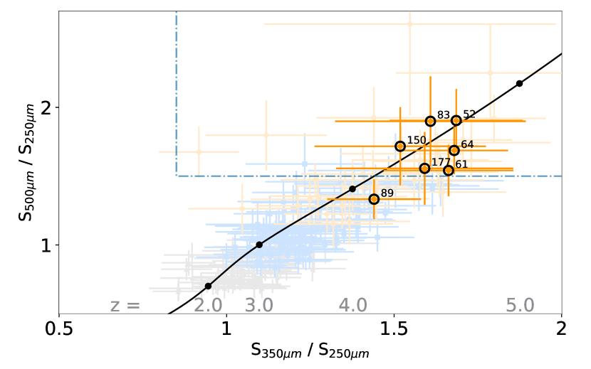
Figure 1: The S${}_{\rm 500~{}\mu m}$/S${}_{\rm 250~{}\mu m}$ vs. S${}_{\rm 350~{}\mu m}$/S${}_{\rm 250~{}\mu m}$ colour-colour plot of our selected sources (open, orange dots) from Herschel/SPIRE observations. The shaded points represent the total HerBS sample (grey, z_phot $<$ 2.5; blue, 2.5 $<$ z_phot $<$ 3.0; orange, z_phot $>$ 3.0). The solid black line indicates the redshift evolution of the spectrum derived from 24 HerBS sources with spectroscopic redshifts (Bakx et al., 2018), and the dash-dotted line indicates the selection criterion for ultra-red sources (Ivison et al., 2016).

3 Observations and Data Reduction

3.1 IRAM EMIR

Using the multi-band heterodyne receiver EMIR, we started our redshift search at IRAM in the 3 mm window (E0: $73-117$ GHz). This window is guaranteed to contain at least one CO line for the redshift ranges 1.2 $<$ z $<$ 2.15 and z $>$ 2.3, where our sources are expected to lie. After the first line detection, we retune mainly to the 2 mm window (E1: $125-184$ GHz) to confirm the spectroscopic redshift via the detection of a second CO line. As backend we used the fast Fourier Transform Spectrometer (FTS200) with a 200 kHz resolution. Observations were carried out mainly in visitor mode, as real-time line confirmations and/or adjustments of the observing strategy were essential. The telescope was operated in position-switching mode, in order to subtract atmospheric variations. Our IRAM observations were carried out in four separate programs, from 2015 until 2017; 080-15 (PI: Helmut Dannerbauer), 079-16, 195-16 and 087-18 (PI: Tom Bakx). These observations took place with good to acceptable weather conditions, for details see Table 2.

Table 2: IRAM 30 m observations

Source	Dates	Time per setup [h]	taueff
HerBS-52	28+29/07/15 03/08/15	13.4 (E0: 9.7; E1: 3.7)	0.03 - 0.6
HerBS-61	06+27/07/16 20+21/10/16 10/04/17	9.2 (E0: 4.0; E1: 5.2)	0.05 - 0.8
HerBS-64	20+21/05/17 29:31/07/15 01/08/15	12.8 (E0: 10; E1: 2.8)	0.02 - 0.6
HerBS-83	26/07/16 20/10/16 27/11/16	15.5 (E0: 14.85; E1: 0.6)	0.02 - 0.4
	06+09+13/04/17 16:22+23/05/17
HerBS-89	20/05/17	1.6 (E0: 1.6)	0.05 - 0.15
HerBS-150	06/07/16 20+21/10/16 12+13/04/17 21/05/17	5.0 (E0: 4.0, E0+E1: 1.0)	0.05 - 0.58
HerBS-177	06+11/07/16 20+21/10/16 28/11/16 06+12/04/17	9.8 (E0: 7.3; E1: 2.5)	0.03 - 0.6

Notes: Col-  (1): HerBS-ID. Col. (2): Dates of observation. Col. (3): Observing time per source and band. Col- (4): Tau corrected for elevation.

We reduced the IRAM data using the GILDAS package CLASS and Python, using the modules numpy (Virtanen et al., 2019), astropy (Astropy Collaboration et al., 2013, 2018) and lmfit (Newville, 2019). Initially, we used CLASS to check the data during the observations. Then we used Python to remove the baseline of individual scans, and to remove bad data. After that, we combined the data and redid the baseline removal while masking out the positions of the spectral lines in order to get accurate flux estimates of the spectral lines. Each six minute scan consists of eight 4 GHz subbands, split by horizontal and vertical polarisation. In total, each scan covered 16 GHz — 8 and 8 GHz separated by 8 GHz — in both horizontal and vertical polarisation in one scan. After the baseline-subtraction, we removed bad data by visual inspection of each subband (up to 10% of the data was removed). Typical examples of when a subscan was considered bad data include strong sinusoidal interference, a strong peak, or a baseline that did not appear linear. All good data were then combined into a spectrum with a frequency resolution of $\sim$70 km s^-1, weighted by both the amount of data points which mapped onto this frequency binning, and by the noise level of the subscan:

$$\rm S_{j}=\frac{\sum^{k}{\frac{\sum^{i\in j}{N_{i,k}}}{\rm{VAR}({N_{k}})}}}{\sum^{k}{n_{i\in j}/{VAR}(N_{k})}}.$$ (1)

Here, $\rm S_{j}$ is the lower-resolution spectrum for a source, where j is the frequency index. The subband data, $N_{i,k}$, has $i$ data points, for all $k$ subbands available for each source. VAR$(N_{k})$ is the variance of the subband data (equal to the square of the standard deviation), and $n_{\rm i\in j}$ is the number of data points $i$ that map onto each lower-resolution frequency bin $j$.

The binned spectra increase the per-bin signal-to-noise, and facilitate the identification of spectral lines. Once we found the location of a spectral line in a spectrum, we return to the raw data in order to remove the baseline while masking out the position of the spectral line. We convert from temperature to flux using point source conversion factors at 3 mm (5.9 Jy/K) and 2 mm (6.4 Jy/K). A typical absolute flux calibration uncertainty of 10% is also taken into account.

3.2 GBT VEGAS

Observations of the lower-J CO transitions of HerBS-52 and HerBS-64, for which robust redshifts were measured with EMIR, were carried out using the Robert C. Byrd Green Bank Telescope (GBT). Five observing sessions were conducted in 2016 October through December (GBT program: 16B210, PI: H. Dannerbauer), and two observing sessions were carried out in 2018 March (GBT DDT program: 18A459, PI: T. Bakx). For HerBS-52, we observed CO(1-0) in K-band and CO(3-2) in W-band (Table 3), while for HerBS-64 CO(1-0), CO(2-1), and CO(3-2) were observed in K, Q, and W-band respectively. All observations used the Versatile GBT Astronomical Spectrometer (VEGAS) with a bandwidth of 1500 MHz and a raw spectral resolution of 1.465 MHz, which provided sufficient velocity coverage and velocity resolution for all bands. For the K- and W bands, the NOD observing mode was adopted. This mode alternates observations between two beams by moving the telescope. For the Q-band, we used the SubBeamNod observing mode which moves the sub-reflector to alternate observations between two beams. SubBeamNod observations allow for faster position switched observations and yield better baselines for receivers whose beam separations are small (e.g., the Ka-band, Q-band, and Argus instruments on the GBT). For K- and W-bands, NOD observations yield better baselines. A nearby bright continuum source was used to correct the pointing and focus of the telescope every 30 to 60 minutes, depending on the observing frequency and conditions. For observations with Q and W-band, the surface thermal corrections for the telescope were made using the AutoOOF observations of 3C273. This method adjusts the surface actuators of the telescope for the current conditions to improve the aperture efficiency at high frequency. The pointing of the telescope as well as the methods for correcting the surface work best in night time under stable thermal conditions. The CO(3-2) observations for HerBS-52 were taken in the afternoon under very clear, sunny skies which greatly degraded the quality of these data. During the afternoon with clear skies, the changing of the surface and the structure yield large effective telescope losses at W-band.

The GBT spectral-line data were reduced using GBTIDL. Each individual NOD and SubBeamNod scan was visually inspected for the two polarisations and two beams. Low-order polynomial baselines were removed and scans showing large residual baseline features were removed before data co-addition. The data were corrected for atmospheric losses. This correction was particularly large for the CO(3-2) data of HerBS-64 since the observed frequency of 68.6 GHz is within the wing of the strong atmospheric O₂ band. The data were corrected for drifts in pointing by using the measured pointing offsets and assuming a Gaussian beam. The absolute flux density scales for the K-band and Q-band observations were derived from observations of 3C286 based on the VLA calibration results of Perley & Butler (2013). For W-band, we used observations of 3C273 and the known flux density as a function of time provided by the ALMA Calibrator Source Catalog online database. Factoring in estimates of all errors, including the uncertainty on the calibration scales, measurement errors, uncertainty for the atmosphere correction, and the uncertainty associated with the pointing and focus drifts, we estimated flux uncertainties errors of 15% at K-band, 20% at Q-band, 40% at W-band for HerBS-64, and 60% at W-band for HerBS-52. The calibration at W-band was particularly challenging for HerBS-52 due to the sunny afternoon conditions which significantly impacted the ability to derive accurate telescope corrections.

3.3 Spectral line measurements

Figure 2: Rest-frame sub-mm spectra of the four sources with confirmed spectroscopic redshifts obtained with the EMIR instrument at the IRAM 30 m telescope. The orange lines mark the detected spectral lines of each galaxy.

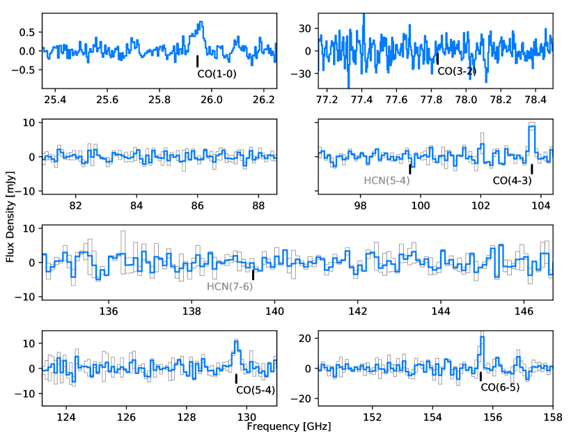
Figure 9: The complete spectra taken of source HerBS-52. We show the spectra at 70 km/s for individual polarisations (grey) and combined polarisations (blue).

We provide all spectra from the IRAM 30m and GBT observations in the Appendix Figures 9 to 15, where we show the spectra at 70 km/s in individual polarisations (grey) and combined polarisations (blue). We initially identified the lines by eye, ensuring the line is detected in both polarisations (grey lines in Fig. 9 to 15). We extract the line properties from the EMIR spectrum binned at a velocity resolution of 70 km/s. In order to estimate the uncertainty on our spectral line parameters, we create 1000 realisations of the spectrum to which we have added artificial noise, based on the standard deviation of the spectrum away from the spectral line. We fit a Gaussian profile to each of these 1000 realisations, which gives us one thousand estimates for each line parameter: frequency, integrated flux and velocity width. We fit the distribution of the thousand data points for each line parameter by a Gaussian, where the central position of the Gaussian is our best estimate for the parameter, and the standard-deviation of this Gaussian function is an accurate measure for the uncertainty. This allowed us to extract the line properties of detections down to a signal-to-noise ratio of $\gtrsim 3\sigma$ from the velocity-integrated flux density.

We present the results of the observations in Table 3. For four sources, we obtained a secure spectroscopic redshift based upon multi-line detections, which always required observations in both the 3 and 2 mm windows. Almost all detected lines are from CO, and in addition we detect for one source the [C i](1-0) line and for one source a water line (H₂O 2₁₁-2₀₂). For the J $>3$ CO observations at the IRAM 30m, we derive velocity-integrated fluxes I_CO from 1.5 to 13 Jy km s^-1, while our lower-J transitions (J $\leq$ 3), observed with the GBT range between 0.1 and 0.8 Jy km s^-1. We do not correct for CMB effects (e.g. observation contrast and enhanced CO excitation), since this requires extensive modelling of the ISM conditions, and exceeds the scope of this paper (da Cunha et al., 2013; Zhang, et al., 2016). We show the rest-frame spectra of the sources with spectroscopic redshifts in Figure 2. The velocity-width FWHM of our sources ranges between 250 and 750 km/s. For each galaxy with a confirmed spectroscopic redshift, we detect the CO(4-3) transition. For three sources of our sample, we were not able to identify a robust spectroscopic redshift, given the spectral lines detected for each source. Instead, we list their spectral line properties in Table 4.

Table 3: Confirmed spectral lines

Source	Redshift	Transition	Frequency [GHz]	ICO [Jy km/s]	FWHM [km/s]	S/N
HerBS-52	3.4419 $\pm$ 0.0006	CO(1-0)	25.951 $\pm$ 0.004	0.39 $\pm$ 0.06	519 $\pm$ 85	6.5
		CO(3-2)	77.854	$<$ 3.52
	3.4428 $\pm$ 0.0005	CO(4-3)	103.783 $\pm$ 0.012	6.07 $\pm$ 0.70	507 $\pm$ 52	8.7
	3.4423 $\pm$ 0.0006	CO(5-4)	129.744 $\pm$ 0.017	6.52 $\pm$ 0.95	515 $\pm$ 72	6.9
	3.4409 $\pm$ 0.0005	CO(6-5)	155.742 $\pm$ 0.016	6.22 $\pm$ 1.52	229 $\pm$ 33	4.1
HerBS-61	3.7275 $\pm$ 0.0005	CO(4-3)	97.532 $\pm$ 0.011	5.66 $\pm$ 0.87	456 $\pm$ 88	6.5
		[C i](1-0)	104.086 $\pm$ 0.066	$<$ 3.63
	3.7271 $\pm$ 0.0006	CO(6-5)	146.312 $\pm$ 0.018	2.25 $\pm$ 0.62	247 $\pm$ 41	3.6
HerBS-64	4.0484 $\pm$ 0.0009	CO(1-0)	22.833 $\pm$ 0.004	0.18 $\pm$ 0.05	310 $\pm$ 81	3.6
	4.0462 $\pm$ 0.0006	CO(2-1)	45.686 $\pm$ 0.005	0.51 $\pm$ 0.12	455 $\pm$ 79	4.3
		CO(3-2)	68.630 $\pm$ 0.017	$<$ 0.49
	4.0473 $\pm$ 0.0007	CO(4-3)	91.352 $\pm$ 0.013	2.06 $\pm$ 0.53	364 $\pm$ 99	3.9
	4.0471 $\pm$ 0.0005	CO(6-5)	137.035 $\pm$ 0.015	2.40 $\pm$ 0.58	331 $\pm$ 123	4.1
	4.0431 $\pm$ 0.0009	H2O 211-202	149.122 $\pm$ 0.027	1.60 $\pm$ 0.54	345 $\pm$ 73	3.0
		CO(7-6)	159.902	$<$ 1.69
		[C i](2-1)	160.457	$<$ 1.69
HerBS-177	3.9633 $\pm$ 0.0006	CO(4-3)	92.898 $\pm$ 0.011	4.35 $\pm$ 1.03	490 $\pm$ 204	4.2
	3.9616 $\pm$ 0.0009	[C i](1-0)	99.187 $\pm$ 0.018	2.00 $\pm$ 0.60	308 $\pm$ 102	3.3
	3.9673 $\pm$ 0.0007	CO(6-5)	139.236 $\pm$ 0.019	7.05 $\pm$ 0.70	677 $\pm$ 62	10

Notes: Col. (1): HerBS-ID. Col. (2): spectroscopic redshift. Col. (3): spectral line. Col. (4): observed frequency. Col. (5): integrated flux of spectral line, for unobserved lines we assume a line width of 500 km/s and a 3 $\sigma$ upper limit. Col. (6): line width expressed in full-Width at half-maximum (FWHM). Col. (7): signal-to-noise ratio of the spectral line.

Table 4: Unconfirmed spectral lines

Source	Frequency [GHz]	ICO [Jy km/s]	FWHM [km/s]	S/N
HerBS-83	89.594 $\pm$ 0.018	2.98 $\pm$ 0.49	636 $\pm$ 82	6.1
	93.235 $\pm$ 0.070	1.84 $\pm$ 0.69	255 $\pm$ 96	2.7
	101.759 $\pm$ 0.022	2.57 $\pm$ 0.54	539 $\pm$ 93	4.8
HerBS-150	83.466 $\pm$ 0.024	13.1 $\pm$ 3.63	635 $\pm$ 117	3.6
	94.089 $\pm$ 0.288	2.06 $\pm$ 0.78	580 $\pm$ 111	2.6

Notes: Col. (1): HerBS-ID. Col. (2): observed frequency. Col. (3): integrated flux of spectral line, for unobserved lines we assume a line width of 500 km/s and a 3 $\sigma$ upper limit. Col. (4): line width expressed in full-Width at half-maximum (FWHM). Col. (5): signal-to-noise ratio of the spectral line.

4 Spectroscopic redshifts

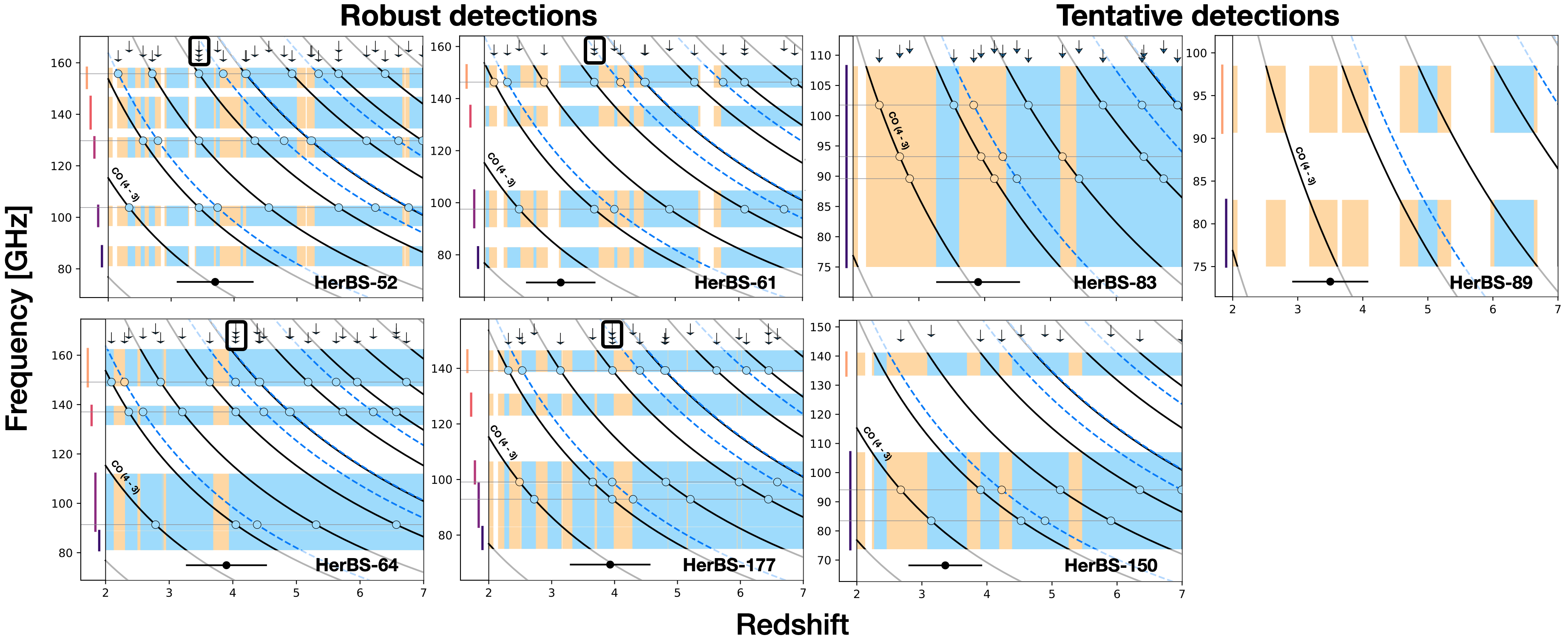
Figure 3: The observed frequency against the covered redshift for all sources, separated between robustly-detected redshifts (left-hand side) and ambiguous redshifts (right-hand side). For each potentially-observed spectral line (CO: black line, H₂O and [C i]: dashed blue line), we show their observed frequency as a function of redshift. On the left-hand-side, we show the observed bandwidth, and indicate at which redshifts we would have expected to detect 1 CO-line (orange fill) or multiple CO-lines (blue fill). We indicate the frequencies of the observed spectral lines with horizontal lines, and indicate the corresponding potential redshifts for each line with an arrow in the top of the graph, with the photometric redshift estimate at the bottom of each graph. For the robust detections, we note that these arrows line up at the robust redshift identification, encircled with a black line. If the redshift is not robustly-identified, the redshift possibilities within the blue fill, e.g. expected multiple CO-line detection, can be excluded, as this would have resulted in multiple line detections. This graphical method removes the need for unwieldy and error-prone comparisons of spectral lines, and graphically shows the frequencies that need to be probed in future missions.

We discuss an efficient graphical analysis to identify the spectroscopic redshift solutions of our sources in Section 4.1. In Section 4.2, we implement this method on the sources with a robust redshift solution and discuss the sources individually. In Section 4.3, we discuss the sources without a robust spectroscopic redshift identification, and provide potential explanations for their non-identification. We conclude this section with a brief discussion on future spectroscopic redshift searches in Section 4.4.

4.1 Graphical analysis for unambiguous spectroscopic redshift identification

We adopt a relatively conservative approach in our identification of our spectroscopic redshifts, demanding a robust spectroscopic redshift via at least two spectral lines. This requires the cross-comparison of multiple redshift possibilities for each detected spectral line. Numerically solving this cross-comparison is a tedious approach, prone to errors and overlooked options. Instead, we use the following graphical method for identifying the potential spectroscopic redshifts for each line. Moreover, the method can be used for sources with only one line detection in order to determine the frequency ranges that need to be probed in future redshift searches.

In Figure 3, we show this graphical method for all observed sources as a collage, separated between the sources with unambiguous (left) and ambiguous redshift identifications (right). In each plot, we show the observed frequency against the covered redshift. We expect to detect CO-lines, and potentially [C i] and H₂O lines, which we graph as black and dashed blue lines, respectively. Each actually-observed spectral line is indicated with a horizontal line at the observed frequency, and where they cross the redshifted spectral lines, we mark the potential spectroscopic redshift with a circle and identify this potential spectroscopic redshift with an arrow in the top of the graph. On the left-hand side, we indicate the observed frequency bands within which we expect to detect all CO-lines. For this range of frequency coverage, we indicate whether the observations would be able to observe one or more spectral lines, indicated with orange and blue fill, respectively. We do this only for the CO lines, as we cannot be sure we would have detected the [C i] and H₂O emission. The black point below indicates the photometric redshift estimate, with its typical uncertainty in $\Delta z/(1+z)$ $\sim$  of 13% (Bakx et al., 2018).

The top arrows line up when multiple lines agree on a robust redshift, identifying the spectroscopic redshift, marked for the sources with unambiguous redshifts with a black border. This check is important, because CO-line redshift surveys can suffer from potential multiple redshift solutions, since the CO-ladder increases linearly with each transition J_up. For example, the observation of J_up = 2 and 4 CO-line transitions of a z = 2 galaxy (76.7 and 153 GHz, resp.) could also be interpreted as the J_up = 3 and 6 CO-line transitions of a z $\approx$ 3.5 galaxy. This mis-identification is a non-negligible possiblity given the 13% errors in sub-mm derived photometric redshifts of around $\Delta z$ $\sim$ 1 (e.g. Pearson et al. 2013; Ivison et al. 2016; Bakx et al. 2018). Using Figure 3, we can confidently exclude other redshift possibilities for the sources with robust redshift identifications, or identify the need for extra observations to be carried out.

4.2 Robust redshifts

Table 5: Physical properties of sources with robust spectroscopic redshifts.

Source	zspec	$\Delta$z/(1+z)	$\mu$LFIR	Tdust	$\mu$Mdust
			log [L⊙]	[K]	[109 M⊙]
HerBS-52	3.4419 $\pm$ 0.0002	-0.058	13.53	30.7	2.7
HerBS-61	3.7273 $\pm$ 0.0004	0.120	13.60	34.6	1.9
HerBS-64	4.0462 $\pm$ 0.0003	0.021	13.66	34.5	2.7
HerBS-177	3.9644 $\pm$ 0.0004	0.007	13.58	32.7	2.9

Notes: Col. (1): HerBS-ID. Col. (2): Spectroscopic redshift calculated from all spectral lines using equation 2. Col.(3): Error in photometric redshift estimate, given by (z_spec - z_phot)/(1+z_spec). Col. (4): Logarithm of the far-infrared bolometric luminosity, integrated from 8 to 1000 $\mu$m. Col. (5): Average temperature, assuming a single temperature grey-body with $\beta$ = 2.

For each source with a consistent spectroscopic redshift identification, we estimate the average spectroscopic redshift, $\bar{z}$, based on a weighted average of the redshifts of each of the lines, $\rm z_{i}$, combined with the redshift uncertainty in each line, $\rm dz_{i}$,

$$\rm\bar{z}=\sqrt{\frac{\sum^{i}{\left(z_{i}/dz_{i}\right)^{2}}}{\sum^{i}\left(1/dz_{i}\right)^{2}}}.$$ (2)

We list spectroscopic redshift per source in Table 5.

HerBS-52: We initially detected a spectral line at 103.783 GHz in the E0 band, which placed the galaxy at either $z=2.3,3.4,$ or $4.5$. The detections of two lines in the E1 range, at 129.744 GHz and 155.742 GHz, yielded a robust spectroscopic redshift of $z_{\rm CO}=3.4419$. This established the detected lines as CO(4-3), CO(5-4), and CO(6-5). This is one of two sources in our sample with subsequent GBT follow-up of the CO(1-0), and CO(3-2) transitions. We detected the CO(1-0), however the GBT observations of the CO(3-2) line had poor baselines, and hence failed to result in a detection. As a result of this, the flux upper limit we derive for the CO(3-2) line of HerBS-52 is too low, as we will discuss in Section 5.4.

HerBS-61: We initially detected a spectral line at 97.532 GHz in our first tuning in E0, which placed the galaxy at either $z=2.5,3.7$ or $4.9$. In the subsequent E1 tuning we detected a spectral line at 146.312 GHz, resulting in a spectroscopic redshift of $z_{\rm CO}=3.7273$. This established the detected lines as CO(4-3) and CO(6-5). We are also able to provide an upper-limit on the neighbouring [C i](1-0) line integrated flux. Note that we can reject the redshift solution at $z=6.1$, since there is no emission line at $\sim$81.3 GHz.

HerBS-64: We initially detected a spectral line at 91.352 GHz after two tunings in the E0 band, which placed the galaxy at either $z=2.8$ or $4.0$. This was followed by two tunings in E1, where we detected a spectral line at 137.035 GHz, which yielded a spectroscopic redshift of $z_{\rm CO}=4.0462$. This established the detected spectral lines as CO(4-3) and CO(6-5). We are also able to provide an upper limit for the CO(7-6) and [C i](2-1) line. This is one of two sources in our sample with subsequent GBT follow-up of the CO(1-0), CO(2-1), and CO(3-2) transitions. The CO(1-0) and CO(2-1) lines are detected clearly with the GBT, however the observations of the CO(3-2) line of HerBS-64 were impacted by high T_sys and opacity, since the line is on the wing of the atmospheric O₂ line. We failed to detect the CO(3-2) emission, and thus we decided to leave this spectral line out in our further analysis.

HerBS-177: We initially detected a spectral line at 92.898 GHz after two tunings in the E0 band, with a $\sim$3$\sigma$ detection at 99.187 GHz, which placed the galaxy at $z=3.9$, although $z=2.7$ and $5.2$ were also possible. In the subsequent E1 tuning we detected a spectral line at 139.236 GHz, yielding a spectroscopic redshift of $z_{\rm CO}=3.9644$. We excluded a potential solution at z = 4.8 because of the lack of CO-emission at $\sim$79 GHz. This established the detected spectral lines as CO(4-3), [C i](1-0), and CO(6-5).

4.3 HerBS sources without spectroscopic redshift

HerBS-83: We observed both tunings in E0 for this source for a significant time (14.7 h in total), revealing several spectral lines. We detected three spectral lines over the entire E0 band, at 89.594, 93.235, and 101.759 GHz. As can be seen in Figure 3, none of these lines agree with a single redshift solution. In the case that each bandwidth was deep enough to detect all possible spectral lines, we can exclude all blue redshift regions in Figure 3, in which we would have at least detected two spectral lines. This removes the z = 4.3 and 3.4 possibilities.

HerBS-89: The lack of observing time – 1.6 hours in a single E0 tuning – on this source did not result in a significant line detection. However, a recent NOEMA study of 13 bright Herschel-selected sources by Neri et al. (2020) revealed the spectroscopic redshift of HerBS-89 to be $z=2.950$.

HerBS-150: The first E0 tuning was observed significantly longer than the other tuning in E0 (4h vs. 1h). The deeper tuning revealed a potential spectral line at 83.466 GHz (signal-to-noise (S/N) $\sim$ 3.5), and the shallow observation also detected a spectral line at 94.089 GHz (S/N $\sim$ 3). The frequencies of these spectral lines, however, do not agree with a single redshift. The E1 tuning has not been observed long enough for us to exclude any of the redshift possibilities.

For three of our sources, we could not find a conclusive spectroscopic redshift. For HerBS-89, this is due solely to a lack of observation time spent on this source. However, for sources HerBS-83 and -150, we find several possible spectral lines (S/N $\sim$ 3), with inconclusive redshifts associated with them. This could point to several sources in a line-of-sight (LOS) alignment blended into a single sub-mm source in the Herschel selection image. A high fraction of bright Herschel sources are gravitationally lensed (e.g. Negrello et al. 2010), potentially causing us to observe the foreground, lower-redshift source together with the background source. Theoretically, Hayward et al. (2013) found the possibility for LOS blending to be larger than the possibility of spatially associated blending ($\Delta z<0.02$), though this is a source of controversy. Observationally, in one extreme case, Zavala et al. (2015) found one of their sources to actually be three LOS blended sources, which could be a similar situation to HerBS-83. However, more follow-up on these three sources are needed, both in band E0 and E1.

4.4 Current and future high-redshift searches

The combination of the large collecting area of the IRAM 30 m telescope and the real-time data analysis enables us to find a CO line within around ten hours of observing time and subsequently confirm the redshift via the detection of a second line for these extremely luminous, mostly lensed sources. Higher-J (J_up $\geq$ 6) CO-lines are necessary for the robust redshift determination of high-redshift sources (z $>$ 3.5) within the 2 and 3 mm windows. Their line luminosities depend strongly on the internal properties of the galaxies, making these luminosities unpredictable. This can cause follow-up programs to suffer from biases towards sources with bright high-J CO-lines, which is indicative of thermalised systems and AGN.

Identifying spectroscopic redshifts with atomic spectral lines could help us, as [CII], [OI], [OIII] and [NII] are typically more luminous than the CO-lines. These atomic spectral lines are typically at slightly shorter wavelengths (e.g. $\lambda$ $<$ 1 mm for [CII] at $z<5.3$). ALMA (e.g. Laporte et al. 2017 and Tamura et al. 2019) and the Herschel SPIRE FTS (George et al., 2013; Zhang et al., 2018) have demonstrated the viability of finding redshifts with atomic lines at high redshift, and new instruments are under development which will probe this regime with enough bandwidth to increase the speed of redshift searches. The upgrade to ZEUS, ZEUS-2, has already demonstrated a significant increase in the bandwidth (Ferkinhoff et al., 2014; Vishwas et al., 2018). The relatively new technology, so-called Microwave Kinetic Inductance Detectors (M-KIDs — Yates et al. 2011), promises a similar increase in bandwidth, with the added versatility, and a significant decrease in instrument size and complexity. Instruments such as DESHIMA (Endo et al., 2012, 2019) and MOSAIC (Baselmans et al., 2017) may allow 10m-class telescopes to compete with ALMA in redshift searches. This evolution in detector technology comes in a time when new telescopes are envisaged, such as the 50m-class telescope AtLAST/LST (Kawabe et al., 2016), CCAT-prime and the SPICA space mission. To summarize, this promises a future where entire sub-mm samples can be followed-up with sub-mm spectroscopy, offering a less biased view of extreme star-forming galaxies.

Redshift searches with interferometers such as ALMA and NOEMA, have also been conducted (e.g. Weiß et al. 2013; Fudamoto et al. 2017; Neri et al. 2020) and are currently ongoing (e.g. $z$-GAL, PIs: Cox, Bakx and Dannerbauer). These telescopes achieve reliable spectral line detections ($\sigma>10$) of lensed SMGs with only very short on-source integration times (several minutes). This sensitivity is due to the large combined collecting area of the array, and also due to their smaller collective beam size, which is similar to the typical size of the target sources ($\sim 1-2$″). This increases the sensitivity of the observation, since most emission of the source is contained within one beam, while collecting fewer photons from sources of noise, such as the atmosphere or the cosmic infrared background. These deep observations can negate the effect of biases, by ensuring even relatively faint high-J CO lines are observed. The high demand for these institutes compared to the small availability of observation time requires optimised tuning set-ups, which can be found by maximising towards multiple-line detections (blue fill in Figure 3) within the redshift region one expects the sources to be.

5 Physical properties

In Section 5.1, we use the spectroscopic redshift to calculate the rest-frame wavelength of the photometry, and use it to derive dust temperatures and dust masses. In Section 5.2, we calculate the luminosity of the spectral lines, in order to calculate the molecular gas masses. We compare the molecular gas masses to the dust mass and star formation rate in Section 5.3. In Section 5.4, we compare the CO spectral line energy distributions (SLEDs). We briefly look at the effect of gravitational lensing on these SLEDs in Section 5.5. Finally, we investigate the gravitational lensing of the sources in Section 5.6.

Table 6: Physical properties based on detected spectral lines

Source	Transition	$\mu$L${}^{\prime}_{\rm specline}$	$\mu$L${}^{\prime}_{\rm{CO(1-0)}}$	$\mu$Mmol	tdep	$\delta$
		[1010 K km/s pc2]	[1010 K km/s pc2]	[1010 M⊙]	[Myr]
HerBS-52	CO(1-0)	20.1 $\pm$ 3.1	20.1 $\pm$ 3.1	16.1 $\pm$ 2.4	24	60
	CO(4-3)	19.7 $\pm$ 2.3	48.0 $\pm$ 5.7	38.4 $\pm$ 4.6	57	142
	CO(5-4)	13.5 $\pm$ 1.8	42.3 $\pm$ 5.6	33.8 $\pm$ 4.5	50	125
	CO(6-5)	9.0 $\pm$ 2.0	42.7 $\pm$ 9.5	34.1 $\pm$ 7.6	51	126
HerBS-61	CO(4-3)	20.8 $\pm$ 2.9	50.8 $\pm$ 7.1	40.7 $\pm$ 5.7	72	214
	[C i](1-0)	$<$ 10.7		$<$160	$<$288
	CO(6-5)	3.7 $\pm$ 0.9	17.5 $\pm$ 4.4	14.0 $\pm$ 3.5	25	74
HerBS-64	CO(1-0)	11.9 $\pm$ 2.3	11.9 $\pm$ 2.3	9.51 $\pm$ 1.83	12	35
	CO(2-1)	8.1 $\pm$ 1.2	9.68 $\pm$ 1.4	7.75 $\pm$ 1.12	10	29
	CO(3-2)	6.3 $\pm$ 2.2	12.1 $\pm$ 4.3	9.68 $\pm$ 3.45	13	36
	CO(4-3)	8.6 $\pm$ 2.0	21.0 $\pm$ 5.0	16.8 $\pm$ 4.0	22	62
	CO(6-5)	4.5 $\pm$ 1.0	21.3 $\pm$ 4.6	17.0 $\pm$ 3.7	22	63
	H2O 211-202	2.5 $\pm$ 0.8
	CO(7-6)	$<$ 2.1	$<$ 11.7	$<$ 9.36	$<$ 12	$<$ 35
	[C i](2-1)	$<$ 2.1		$<$ 21	$<$27
HerBS-177	CO(4-3)	17.7 $\pm$ 3.8	43.1 $\pm$ 9.2	34.5 $\pm$ 7.4	51	119
	[C i](1-0)	7.1 $\pm$ 1.9		106 $\pm$ 29	159
	CO(6-5)	12.7 $\pm$ 1.2	60.6 $\pm$ 5.5	48.5 $\pm$ 4.4	72	167

Notes: Col. (1): Source name. Col. (2): CO transition. Col. (3): Line luminosity without magnification correction. Col. (4): Predicted CO(1-0) line luminosity according to the average CO spectral line energy distribution based on Bothwell et al. (2013). Col. (5): Molecular hydrogen mass in the galaxy, derived from $\alpha$ = 0.8. Col.6): Depletion time is defined as the molecular gas mass divided by the star formation rate found in Table 1. Col. (7): Gas-to-dust ratio, $\delta$, is the molecular gas mass divided by the dust mass.

5.1 Dust temperatures and mass estimates

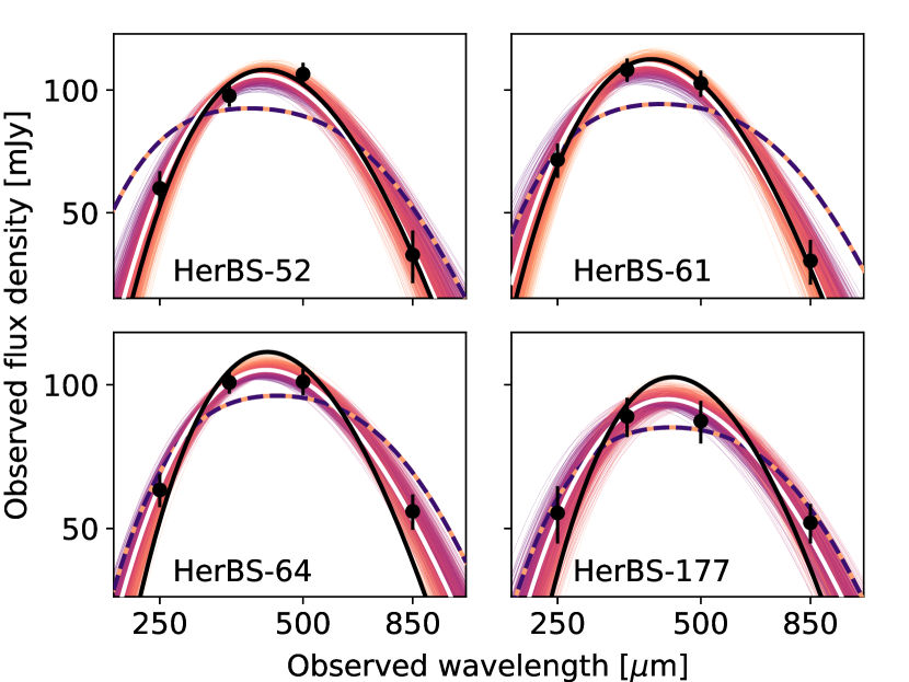
Figure 4: We fit the continuum fluxes (black points) for all sources with spectroscopic redshift for various spectral templates. The dashed line shows the best-fit template from Bakx et al. (2018), which is derived by fitting a two-temperature modified black-body to Herschel/SPIRE and JCMT/SCUBA-2 photometry of 24 HerBS sources with $z_{\rm spec}>1.5$. The black solid line shows the best-fit of a single-temperature modified black-body assuming a dust-emissivity coefficient ($\beta$) of 2. We also show the best-fit spectra of a single-temperature modified black-body, with a variable $\beta$-value, for 1000 iterations of the Monte-Carlo code (purple-to-orange thin lines), where the white line shows the most likely solution.

We use the spectroscopic redshift to calculate the rest-frame wavelength of the photometry of each HerBS source. We use this photometry to fit a dust temperature to our sources, which we show in Figure 4. We fit the photometry for using two different modified black-body templates, for one template, we allow $\beta$ to vary, for the other template, we fix $\beta$ to 2. Here, we use the equations from da Cunha et al. (2013) and Zhang, et al. (2016) to include both the effect of dust heated by the CMB and the effect of the contrast against the CMB emission.

We find dust temperatures between 30 and 35 K, typical for SMGs at z $\sim$ 3.5 (e.g. Jin, et al. 2019), which we show for each source in Table 5. We find similar bolometric luminosities for our sources as detailed in Table 1, calculated by integrating the template from Bakx et al. (2018) from 8 to 1000 $\mu$m rest-frame. We use this template, since it is based on the photometry of similarly-selected sources – detailed in Bakx et al. (2018). We determine the average dust temperature of the sources by fitting a single-temperature modified blackbody, with a $\beta$ of 2.0, to the galaxy.

We use the estimated dust temperature to calculate a total dust mass using

$$M_{d}=\frac{S_{\nu}D_{\rm L}^{2}}{(1+z)\kappa_{\rm rest}B_{\nu}(\lambda_{\rm rest},T_{d})}.$$ (3)

S_ν is the observed flux density, $D_{\rm L}$ is the luminosity distance, $z$ is the spectroscopic redshift, $\kappa_{\rm rest}$ is derived by interpolating the values from Draine (2003), and $B_{\nu}(\lambda_{\rm rest},T_{d})$ is the black-body radiation expected for a $T_{d}$ [K] source at $\lambda_{\rm rest}$. We use the 850 $\mu$m fluxes, as they probe the cold dust component of the spectrum.

We find dust masses of the order $2\times 10^{9}$ M${\odot}$, which are similar to the dust masses found for other high-redshift sources selected from wide-area surveys, such as those in Harrington et al. (2016); Fudamoto et al. (2017) and Yang et al. (2017).

5.2 Molecular gas masses

We detail the line properties in Table 6. We calculate the line luminosity with the equation from Solomon et al. (1997):

$$L^{\prime}=3.25\times 10^{7}S_{\rm CO}\Delta vf_{\rm obs}^{-2}D_{\rm L}^{2}(1+z)^{-3}.$$ (4)

with the integrated flux, $S_{\rm CO}\Delta v$, in Jy km s^-1, the observed frequency, $f_{\rm obs}$, in GHz, and the luminosity distance, $D_{\rm L}$, in Mpc.

We use the line luminosity ratios from Ivison et al. (2011) and Bothwell et al. (2013) to calculate the CO(1-0) line luminosity. The molecular hydrogen mass in the galaxy is calculated using

$$M_{\rm H_{2}}=\alpha L^{\prime}_{\rm CO(1-0)}.$$ (5)

We adopt $\alpha$ = 0.8 $M_{\odot}$/(K km/s pc²). Similar to Harrington et al. (2016); Fudamoto et al. (2017) and Yang et al. (2017), we find molecular gas masses on the order of 10¹¹ M_⊙, not corrected for magnification.

Here, we note the factor of two difference between the CO(1-0)-derived molecular mass for HerBS-52 and -64 compared to the masses derived from the other transitions. The ratios tabulated by Bothwell et al. (2013) over-predict the CO(1-0) luminosity, suggesting that HerBS-52 and -64 are more thermalised than the average source in Bothwell et al. (2013). Since the CO(1-0) fluxes give the most accurate description of the CO-derived molecular gas masses, we note the need for direct CO(1-0) observations to derive accurate molecular gas masses. Moreover, even for HerBS-61 where we only have J $>3$ CO lines, we find a factor of 3 difference in molecular gas mass between the two lines.

We also derive the molecular gas masses from the [C i](1-0) and [C i](2-1) upper limits and the single [C i](1-0) detection. [C i] emission traces the molecular gas more reliably (e.g. Papadopoulos & Greve 2004), however is typically fainter than CO emission. We use the equations from Weiß et al. (2005) and Walter et al. (2011) to calculate the [C i] mass from both the [C i](1-0) and [C i](2-1) line luminosity estimates. Since no sources have both [C i](2-1) and [C i](1-0) observations, we assume that the [C i] excitation temperature is equal to the dust temperature. From Walter et al. (2011), we adopt the average carbon abundance X[C i]/X[H₂] = 8.4 $\times$ 10^-4. For both the upper limits of HerBS-61 and -64, we find molecular gas masses agreeing with the CO-derived molecular gas masses. For HerBS-177, where we have a [C i] line detection, we find double or triple the amount derived from the CO emission. This could be due to large amounts of cold, sub-thermally ionised gas, which are not observable with J $>3$ CO emission (Papadopoulos & Greve, 2004; Papadopoulos, Bisbas & Zhang, 2018). The spread in molecular gas mass estimates indicates the need for high-redshift J $<4$ CO and [C i] observations, although we note the low significance of the [CI](1-0) observation, and the lack of the [CI](2-1) line, which is crucial for the correct excitation temperature. Moreover, the estimated CO-dark gas could change depending on differential lensing effects.

5.3 Gas depletion timescale and gas-to-dust ratio

Gas depletion times, defined as the molecular gas mass divided by the star formation rate (t${}_{\rm dep}=\mu$M_mol/$\mu$SFR), are on the order of tens of millions of years. It is important to note that the star-formation rates are derived from the photometry, which are very dependent on the assumed initial mass function, and can vary significantly (e.g. Tacconi, Genzel & Sternberg 2020). These suggest that these sources are undergoing very short-lived bursts in star formation, or have to be accreting significant amounts of intergalactic gas to sustain this rate of star formation. In the case of HerBS-177, the [C i]-derived molecular gas mass indicates that we are missing the CO-dark molecular gas in our estimates, which could also fuel the star formation and sustain the starburst phase over longer timescales. These time-scales are similar to those found for other high-redshift sources selected from wide-area surveys, such as those in Harrington et al. (2016); Fudamoto et al. (2017) and Yang et al. (2017).

The gas-to-dust ratio, $\delta$, is the molecular gas mass divided by the dust mass. We find ratios of the order tens to hundreds. This is similar to what is seen for local galaxies and high-redshift SMGs (e.g. Dunne et al. 2018).

5.4 CO spectral line energy distribution

Figure 5 shows the velocity-integrated flux I_CO of each CO transition of the sources with identified J-transitions. The CO-ladders of HerBS-52, and -64 appear to peak around $J=5$ or 6, whilst both HerBS-61 and -177 appear to have already sloped downward at or below $J=4$.

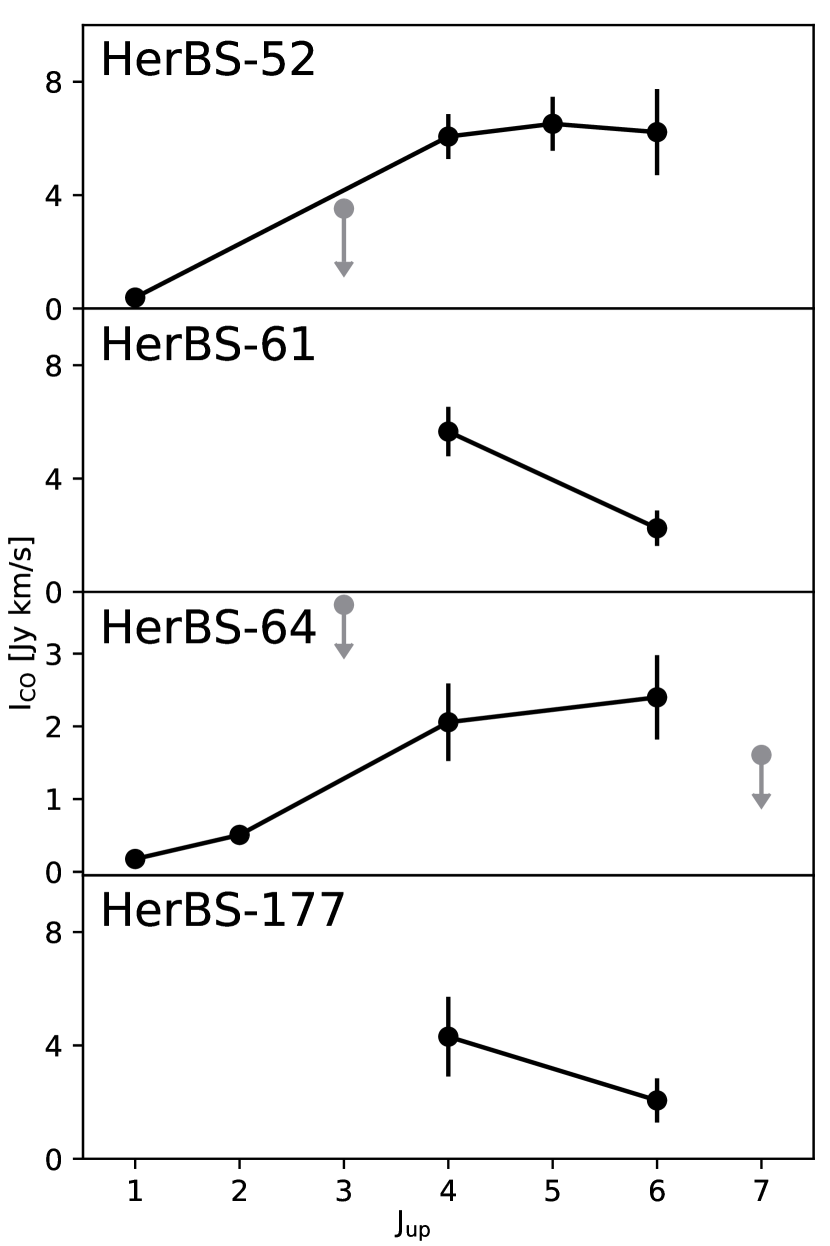
Figure 5: The CO SLED for the four sources from our sample with spectroscopic redshifts. The velocity-integrated flux I${}_{\rm CO_{J_{up},J{up-1}}}$ for each CO transition, J_up, shows the diverse behaviour of the CO spectral line energy distributions within our sample. Arrows indicate upper limits, where the integrated flux is taken to be less than three times the off-line standard deviation, assuming a FWHM of 500 km $s^{-1}$.

Figure 6 shows the integrated flux of each detected CO line of the sources with a spectroscopic redshift. We normalize the CO spectral line energy distribution (CO SLED) to the CO(4-3), as this transition was detected for all sources. We compare the CO SLEDs against two types of SLED profiles. Firstly, the constant brightness profile indicates the theoretical maximum emission in each CO transition, in the case where all excitation states are equally populated. Secondly, we compare against the line ratios of non-lensed SMGs from Bothwell et al. (2013) based on CO(1-0) observations by Riechers et al. (2011) and Ivison et al. (2011), with S_850μm flux densities about 6 to 20 times lower than the sources in our sample.

The slope in Figure 5 and the comparison in Figure 6 show that HerBS-52 and HerBS-64 are more thermalised system (e.g. Weiß et al. 2005; Weiß, et al. 2007; van der Werf, et al. 2010). This is contrasted by HerBS-61 and HerBS-177, which appear to already slope downward, suggestive of a less-thermalised system. We note that the CO(3-2) emission of HerBS-52 suggests a lower flux than expected from a constant-brightness emission, suggesting the upper-limit on the CO(3-2) flux is incorrect due to the poor quality baselines.

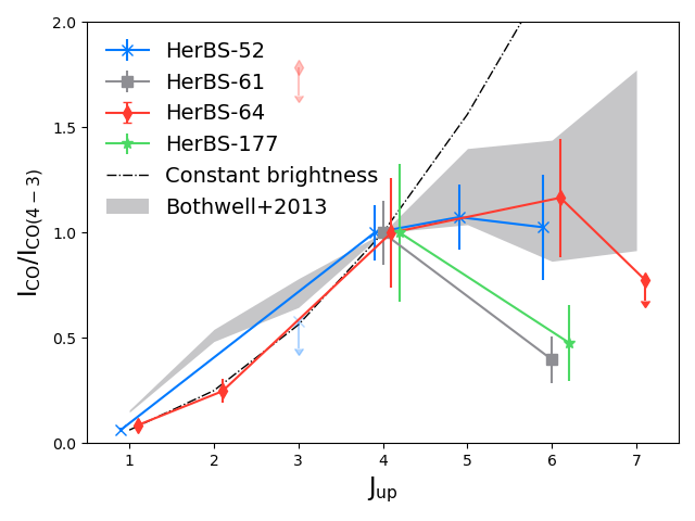
Figure 6: Comparison of the individual CO line luminosity ratios, normalised against CO(4-3), for different J_up. For comparison, we plot against two SLEDS; fully thermalised SLED, and the average SLED of Bothwell et al. (2013).

We derive the line luminosity ratios, $r_{\rm J_{a},J_{b}}$, for each of our sources, using equation

$$r_{\rm J_{a},J_{b}}=\frac{L^{\prime}_{a}}{L^{\prime}_{b}}=\frac{I_{a}}{I_{b}}\frac{J_{b}^{2}}{J_{a}^{2}}.$$ (6)

Here, $L^{\prime}_{a}$ and $L^{\prime}_{b}$ refers to the line luminosity of lines $a$ and $b$, $I_{a}$ and $I_{b}$ refers to the integrated line flux, and $J_{a}$ and $J_{b}$ refer to the upper quantum transition, commonly referred to as $J_{\rm up}$.

For each of our sources, we plot the ratios in Figure 7. We compare the sample to the ratio from Bothwell et al. (2013), and the constant brightness SLED profile.

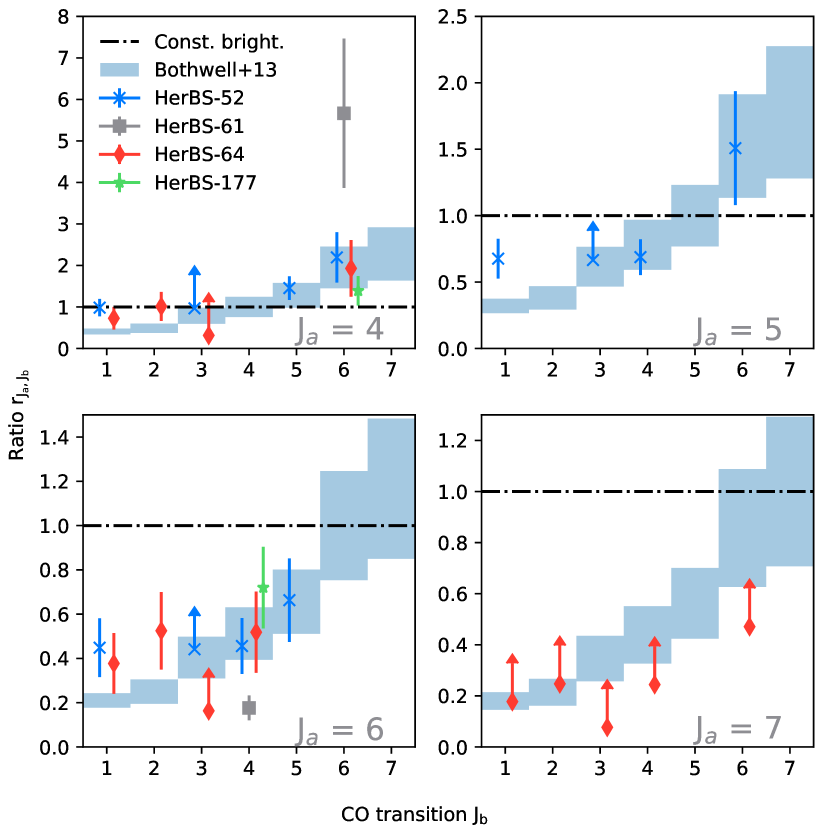
Figure 7: Line luminosity ratios between the different lines are calculated based on the CO-line luminosities using equation 6. We compare the ratios to the expected ratios of the compilation of Bothwell et al. (2013) (blue fill), and the constant brightness profile (dashed line). The constant brightness profile assumes equal excitation among all states, and thus is 1.0 for all transitions.

In general, the fluxes agree with the Bothwell et al. (2013) ratios. The only major outlier is the CO(6-5) flux of HerBS-61, which is significantly fainter than predicted, resulting in a high data point. Notably, the lower-J fluxes of HerBS-52 suggest that these transitions are fully thermalised, while the higher transitions are not. We note that not all source ratios lie within the predicted values of Bothwell et al. (2013), suggesting a large spread in the internal conditions of the ISM.

5.5 Differential lensing

The magnification factor of a strongly-lensed source is dependent on the position of the emission in the source plane (e.g. Serjeant 2012). Since emission at a certain CO transition is determined by the ISM conditions, a different magnification factor between various ISM conditions can skew the analysis of the galaxy, especially for unresolved observations such as these IRAM 30m and GBT observations. Since we suspect our sources are lensed from both optical and near-infrared follow-up (Negrello et al., 2017; Bakx, Eales & Amvrosiadis, 2020), and from the following Section 5.6, we investigate the potential effects of this on our SLED analysis.

Among our sources, both HerBS-52 and HerBS-61 have smaller line widths (FWHM) for their CO(6-5) line, when compared to their lower-J transitions. HerBS-177 actually has a larger velocity width for its CO(6-5) line than the other two spectral lines, although the significance of this velocity difference is smaller. HerBS-64 does not appear to have a large difference in line width, where all lines are within 350 to 450 km/s. Discrepancies among the line widths could suggest differential lensing, although these discrepancies can also be explained by a difference in ISM distribution.

The CO luminosity ratios in Figure 7 provide another indication of differential lensing. The CO(4-3) over CO(6-5) ratio ($r_{\rm 4,6}$) of HerBS-61 is around 1.5$\sigma$ larger than expected from Bothwell et al. (2013). Similarly, both HerBS-52 and HerBS-64 have a higher ratio than expected for the CO(6-5) over CO(1-0) – and over CO(2-1) for HerBS-64 – luminosity ratio ($r_{\rm 6,1}$ and $r_{\rm 6,2}$). Unfortunately, there exists a large degeneracy between the internal ISM conditions and the effects of differential lensing. This is further exacerbated by the low S/N of the spectral lines, which stresses the need for resolved observations.

5.6 Are our sources lensed?

Analogous to the Tully-Fisher relationship (Tully & Fisher, 1977), we compare the CO line width against the line luminosity to find evidence for the lensing nature of our sources (e.g. Harris et al., 2012; Bothwell et al., 2013; Aravena, et al., 2016; Dannerbauer et al., 2017; Neri et al., 2020). Lensing amplifies the apparent CO luminosity, while the line width remains unaffected. Harris et al. (2012) showed that this diagnostic could be used to show that the brightest Herschel galaxies are mostly lensed, with relatively large CO luminosities compared to their velocity widths. In our case, we know that there is a large likelihood of our sources being lensed, as they are selected with 500$\mu$m fluxes around the lensing selection function by Negrello et al. (2010) of $\sim$100 mJy. From previous work (e.g, Ivison et al., 2011; Riechers et al., 2011; Bothwell et al., 2013), we know there exists a significant spread in the conversion of CO(4-3) flux to CO(1-0), and we therefore examine the lensing properties of our sources using the CO(4-3) line, and compare them against sources with detected CO(4-3) fluxes.

Figure 8 shows the CO(4-3) line luminosity of each source plotted versus the Full-Width at Half-Maximum (FWHM) of the line width. We compare against the CO(4-3) luminosity of other SMG samples: the sources from Bothwell et al. (2013), the Planck sources from Harrington et al. (2016) and Cañameras et al. (2015), the brightest Herschel sources from Yang et al. (2017), Zavala et al. (2015) and George et al. (2013), the Hyperluminous LIRG from Ivison et al. (2013), the sources from Neri et al. (2020), and the Cosmic Eyebrow (Dannerbauer, et al., 2019). Finally, we compare against the ultra-red Herschel sources from Fudamoto et al. (2017), explicitly selected to contain a low fraction of lensed sources, aiming to find the most distant dusty starbursts (Ivison et al., 2016), although high-resolution ALMA imaging by Oteo et al. (2017) suggests that $\sim$40% of sources are gravitationally-lensed.

The unlensed relationship between the line luminosity and its velocity width is from Bothwell et al. (2013) (solid line). The dashed line, assuming a magnification factor of $\mu=10$, represents the magnified relation. We note a distinct split between lensed and unlensed sources. All our sources appear to agree with the $\mu=10$ line, and lie within the distribution of previously-observed lensed sources. This suggests that these sources are all magnified by the mass of foreground intervening galaxies.

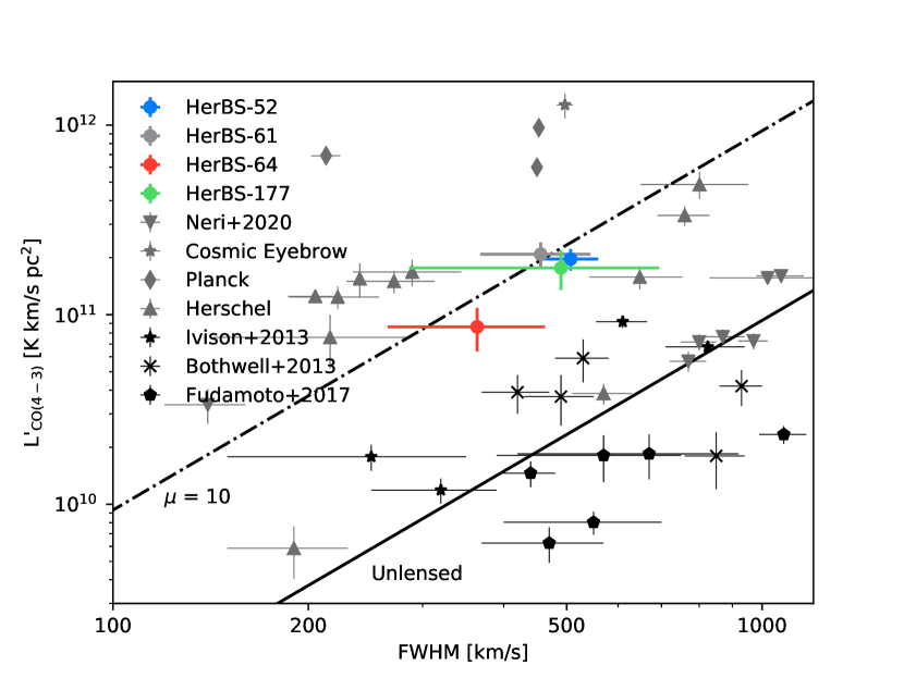
Figure 8: The CO(4-3) line luminosity is shown against the line width for the sources with robust redshift identifications. Their bright line luminosity, compared to their line width, suggests they are gravitationally lensed. Unlensed sources (black symbols) lie close to the solid line from Bothwell et al. (2013), as can be seen for the (predominantly) unlensed sources from Bothwell et al. (2013), Ivison et al. (2013) and Fudamoto et al. (2017). Lensed sources (dark grey symbols), such as known lenses (Cosmic Eyebrow; Dannerbauer, et al. 2019) and the ones selected from the Planck (Cañameras et al., 2015; Harrington et al., 2016) and Herschel surveys (Cox et al., 2011; Zavala et al., 2015; Yang et al., 2017; Neri et al., 2020). These lenses have more apparently-luminous spectral lines, while the gravitational lensing does not affect the line widths. Lensed sources are therefore expected in the upper-left part of this figure.

6 Conclusions

In an effort to characterize the galaxies between the cosmic dawn and cosmic noon, we have targeted 7 bright Herschel sources from the HerBS sample around redshift $z\sim 4$. For four of these sources, we have identified robust spectroscopic redshifts using the IRAM 30m telescope, with redshifts ranging between $z=3.4$ to 4.1. For two of these sources with spectroscopic redshifts, we obtained GBT observations of the J $<$ 4 CO lines. In this redshift search, the use of the 2 mm window proved indispensable to confirm the spectroscopic redshifts using the CO line transitions, as can be seen in our graphical analysis in Figure 3. We therefore recommend using the 2 mm window together with the 3 mm window in future redshift searches. Both a lack of observation time and the potential of source confusion could explain the lack of a robust redshift for the three sources without a spectroscopic redshift identification.

The four sources with spectroscopic redshifts have dust temperatures around 30 to 35 K, and dust masses around 2 $\times$ 10⁹ M_⊙, similar to other sources selected with Planck, Herschel and the South Pole Telescope. We estimated the molecular gas mass in the galaxies using both low-J and high-J CO-lines and using the [C i] line. We find molecular gas masses between 1 and 10 $\times$ 10¹¹ M_⊙, however we note a large discrepancy between the molecular gas masses estimated using different spectral lines. There exists around a factor of 2 discrepancy between the CO(1-0) and J $>3$ CO transitions, stressing the need for CO(1-0) lines to accurately estimate the molecular gas mass. The molecular gas estimate from atomic carbon ([C i]) for one source is several times larger than from CO lines, suggesting the possibility that the majority is CO-dark gas.

The CO SLEDs of the four sources appear different, where HerBS-52 and HerBS-64 have increasing SLEDs, peaking around CO(5-4) or CO(6-5), while HerBS-61 and HerBS-177 appear to have downward-sloping SLEDs, suggesting a peak below CO(4-3). The behaviour of the first two sources is similar to the average behaviour seen in population studies, while the latter two appear slightly discrepant.

We find an indication of gravitational lensing for all four sources with spectroscopic redshifts. The luminosity of the CO line emission is larger than we expect from their line width. This indicates an amplification of the emitted spectral line due to gravitational lensing. This is in line with what we expected, due to the presence of potential foreground galaxies identified in optical and near-infrared studies.

Appendix A Individual spectra

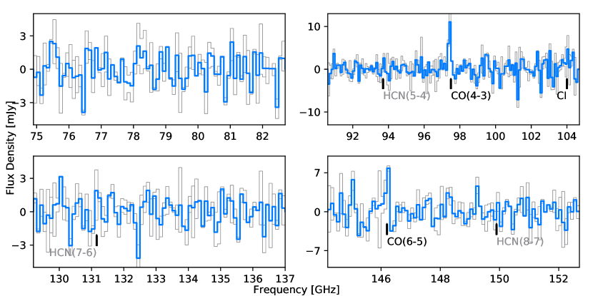
Figure 10: The complete spectra taken of source HerBS-61. We show the spectra at 70 km/s for individual polarisations (grey) and combined polarisations (blue).

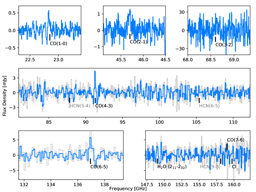
Figure 11: The complete spectra taken of source HerBS-64. We show the spectra at 70 km/s for individual polarisations (grey) and combined polarisations (blue).

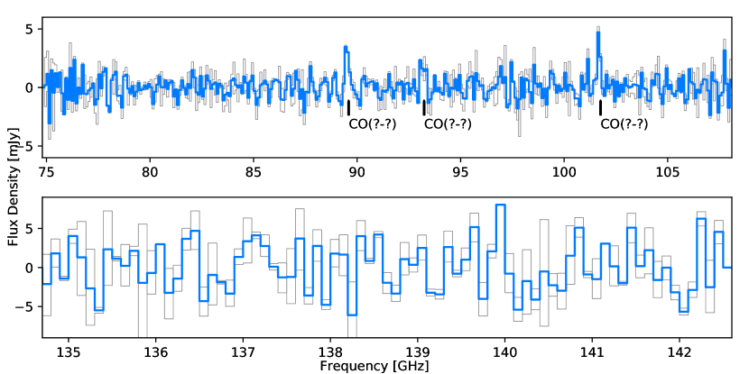
Figure 12: The complete spectra taken of source HerBS-83. We show the spectra at 70 km/s for individual polarisations (grey) and combined polarisations (blue).

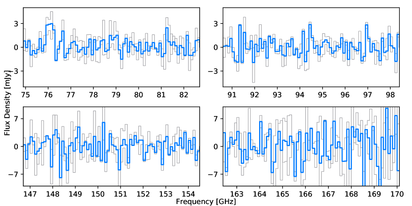
Figure 13: The complete spectra taken of source HerBS-89. We show the spectra at 70 km/s for individual polarisations (grey) and combined polarisations (blue).

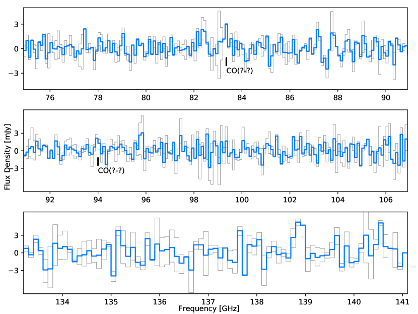
Figure 14: The complete spectra taken of source HerBS-150. We show the spectra at 70 km/s for individual polarisations (grey) and combined polarisations (blue).

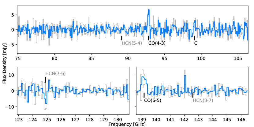
Figure 15: The complete spectra taken of source HerBS-177. We show the spectra at 70 km/s for individual polarisations (grey) and combined polarisations (blue).

References

- Amvrosiadis et al. (2019) Amvrosiadis A., et al., 2019, MNRAS, 483, 4649
- Aravena, et al. (2016) Aravena M., et al., 2016, MNRAS, 457, 4406
- Astropy Collaboration et al. (2013) Astropy Collaboration, et al., 2013, A&A, 558, A33
- Astropy Collaboration et al. (2018) Astropy Collaboration, et al., 2018, AJ, 156, 123
- Bakx et al. (2018) Bakx T. J. L. C., et al., 2018, MNRAS, 473, 1751
- Bakx, Eales & Amvrosiadis (2020) Bakx T. J. L. C., Eales S., Amvrosiadis A., 2020, MNRAS, 493, 4276
- Bakx, et al. (2020) Bakx T. J. L. C., et al., 2020, MNRAS, 494, 10
- Baselmans et al. (2017) Baselmans J. J. A., et al., 2017, A&A, 601, A89
- Blain & Longair (1993) Blain A. W., Longair M. S., 1993, MNRAS, 264, 509
- Blain, et al. (1999) Blain A. W., Smail I., Ivison R. J., Kneib J.-P., 1999, MNRAS, 302, 632
- Bothwell et al. (2013) Bothwell M. S., et al., 2013, MNRAS, 429, 3047
- Bourne et al. (2016) Bourne N., et al., 2016, MNRAS, 462, 1714
- Bouwens et al. (2015) Bouwens R. J., et al., 2015, ApJ, 803, 34
- Cai et al. (2013) Cai Z.-Y., et al., 2013, ApJ, 768, 21
- Cañameras et al. (2015) Cañameras R., et al., 2015, A&A, 581, A105
- Carter et al. (2012) Carter M., et al., 2012, A&A, 538, A89
- Casey et al. (2018) Casey C. M., et al., 2018, ApJ, 862, 77
- Cox et al. (2011) Cox P., et al., 2011, ApJ, 740, 63
- da Cunha et al. (2013) da Cunha E., et al., 2013, ApJ, 766, 13
- Danielson et al. (2011) Danielson A. L. R., et al., 2011, MNRAS, 410, 1687
- Dannerbauer et al. (2002) Dannerbauer H., et al., 2002, ApJ, 573, 473
- Dannerbauer et al. (2004) Dannerbauer H., et al., 2004, ApJ, 606, 664
- Dannerbauer, Walter & Morrison (2008) Dannerbauer H., Walter F., Morrison G., 2008, ApJL, 673, L127
- Dannerbauer, et al. (2019) Dannerbauer H., Harrington K., Díaz-Sánchez A., Iglesias-Groth S., Rebolo R., Genova-Santos R. T., Krips M., 2019, AJ, 158, 34
- Dannerbauer et al. (2017) Dannerbauer H., et al., 2017, A&A, 608, A48
- Dunne et al. (2018) Dunne L., et al., 2018, MNRAS, 479, 1221
- Draine (2003) Draine B. T., 2003, ARA&A, 41, 241
- Eales et al. (2010) Eales S., et al., 2010, PASP, 122, 499
- Edge et al. (2013) Edge A., Sutherland W., Kuijken K., Driver S., McMahon R., Eales S., Emerson J. P., 2013, Msngr, 154, 32
- Endo et al. (2012) Endo A., et al., 2012, SPIE, 8452, 84520X
- Endo et al. (2019) Endo A., et al., 2019, NatAs.tmp, 418
- Erickson et al. (2007) Erickson N., Narayanan G., Goeller R., Grosslein R., 2007, ASPC, 375, 71
- Falgarone et al. (2017) Falgarone E., et al., 2017, Natur, 548, 430
- Ferkinhoff et al. (2014) Ferkinhoff C., et al., 2014, ApJ, 780, 142
- Finkelstein et al. (2015) Finkelstein S. L., et al., 2015, ApJ, 810, 71
- Fixsen, Bennett, & Mather (1999) Fixsen D. J., Bennett C. L., Mather J. C., 1999, ApJ, 526, 207
- Franceschini, et al. (1991) Franceschini A., Toffolatti L., Mazzei P., Danese L., de Zotti G., 1991, A&AS, 89, 285
- Fudamoto et al. (2017) Fudamoto Y., et al., 2017, MNRAS, 472, 2028
- George et al. (2013) George R. D., et al., 2013, MNRAS, 436, L99
- González-Nuevo et al. (2012) González-Nuevo J., et al., 2012, ApJ, 749, 65
- González-Nuevo et al. (2019) González-Nuevo J., et al., 2019, A&A, 627, A31
- Griffin et al. (2010) Griffin M. J., et al., 2010, A&A, 518, L3
- Hayward et al. (2013) Hayward C. C., Behroozi P. S., Somerville R. S., Primack J. R., Moreno J., Wechsler R. H., 2013, MNRAS, 434, 2572
- Harrington et al. (2016) Harrington K. C., et al., 2016, MNRAS, 458, 4383
- Harris et al. (2012) Harris A. I., et al., 2012, ApJ, 752, 152
- Harris et al. (2010) Harris A. I., et al., 2010, ApJ, 723, 1139
- Harris et al. (2007) Harris A. I., et al., 2007, ASPC, 375, 82
- Ivison et al. (2011) Ivison R. J., Papadopoulos P. P., Smail I., Greve T. R., Thomson A. P., Xilouris E. M., Chapman S. C., 2011, MNRAS, 412, 1913
- Ivison et al. (2013) Ivison R. J., et al., 2013, ApJ, 772, 137
- Ivison et al. (2016) Ivison R. J., et al., 2016, ApJ, 832, 78
- Jin, et al. (2019) Jin S., et al., 2019, ApJ, 887, 144
- Kawabe et al. (2016) Kawabe R., Kohno K., Tamura Y., Takekoshi T., Oshima T., Ishii S., 2016, SPIE, 9906, 990626
- Kennicutt & Evans (2012) Kennicutt R. C., Evans N. J., 2012, ARA&A, 50, 531
- Kerr et al. (2014) Kerr A. R., Pan S.-K., Claude S. M. X., Dindo P., Lichtenberger A. W., Effland J. E., Lauria E. F., 2014, ITTST, 4, 201
- Laporte et al. (2017) Laporte N., et al., 2017, ApJL, 837, L21
- de Looze et al. (2011) De Looze I., Baes M., Bendo G. J., Cortese L., Fritz J., 2011, MNRAS, 416, 2712
- Madau & Dickinson (2014) Madau P., Dickinson M., 2014, ARA&A, 52, 415
- Maddox et al. (2018) Maddox S. J., et al., 2018, ApJS, 236, 30
- Magdis et al. (2011) Magdis G. E., et al., 2011, ApJ, 740, L15
- Marrone et al. (2018) Marrone D. P., et al., 2018, Natur, 553, 51
- Naylor et al. (2003) Naylor B. J., et al., 2003, SPIE, 4855, 239
- Negrello et al. (2007) Negrello M., et al., 2007, MNRAS, 377, 1557
- Negrello et al. (2010) Negrello M., et al., 2010, Sci, 330, 800
- Negrello et al. (2017) Negrello M., et al., 2017, MNRAS, 465, 3558
- Neri et al. (2020) Neri R., et al., 2019, 2020, A&A 635, A7
- Newville (2019) Newville M., et al., 2019, Zenodo, 3381550
- Oliver et al. (2012) Oliver S. J., et al., 2012, MNRAS, 424, 1614
- Oteo et al. (2017) Oteo I., et al., 2017, arXiv, arXiv:1709.04191
- Papadopoulos & Greve (2004) Papadopoulos P. P., Greve T. R., 2004, ApJL, 615, L29
- Papadopoulos et al. (2012) Papadopoulos P. P., van der Werf P. P., Xilouris E. M., Isaak K. G., Gao Y., Mühle S., 2012, MNRAS, 426, 2601
- Papadopoulos, Bisbas & Zhang (2018) Papadopoulos P. P., Bisbas T. G., Zhang Z.-Y., 2018, MNRAS, 478, 1716
- Pearson et al. (2013) Pearson E. A., et al., 2013, MNRAS, 435, 2753
- Perley & Butler (2013) Perley R. A., Butler B. J., 2013, ApJS, 204, 19
- Pilbratt et al. (2010) Pilbratt G. L., et al., 2010, A&A, 518, L1
- Planck Collaboration et al. (2016) Planck Collaboration, et al., 2016, A&A, 594, A13
- Poglitsch et al. (2010) Poglitsch A., et al., 2010, A&A, 518, L2
- Riechers et al. (2011) Riechers D. A., Hodge J., Walter F., Carilli C. L., Bertoldi F., 2011, ApJL, 739, L31
- Riechers et al. (2013) Riechers D. A., et al., 2013, Natur, 496, 329
- Riechers et al. (2017) Riechers D. A., et al., 2017, ApJ, 850, 1
- Serjeant (2012) Serjeant S., 2012, MNRAS, 424, 2429
- Smail, Ivison & Blain (1997) Smail I., Ivison R. J., Blain A. W., 1997, ApJL, 490, L5
- Smith et al. (2012) Smith M. W. L., et al., 2012, ApJ, 756, 40
- Solomon et al. (1997) Solomon P. M., Downes D., Radford S. J. E., Barrett J. W., 1997, ApJ, 478, 144
- Spilker et al. (2018) Spilker J. S., et al., 2018, Sci, 361, 1016
- Stacey et al. (2010) Stacey G. J., Hailey-Dunsheath S., Ferkinhoff C., Nikola T., Parshley S. C., Benford D. J., Staguhn J. G., Fiolet N., 2010, ApJ, 724, 957
- Swinbank et al. (2010) Swinbank A. M., et al., 2010, Natur, 464, 733
- Tacconi, Genzel & Sternberg (2020) Tacconi L. J., Genzel R., Sternberg A., 2020, arXiv, arXiv:2003.06245
- Tamura et al. (2019) Tamura Y., et al., 2019, ApJ, 874, 27
- Tully & Fisher (1977) Tully R. B., Fisher J. R., 1977, A&A, 500, 105
- Valiante et al. (2016) Valiante E., et al., 2016, MNRAS, 462, 3146
- Vieira et al. (2013) Vieira J. D., et al., 2013, Natur, 495, 344
- Virtanen et al. (2019) Virtanen P., et al., 2019, zndo
- Vishwas et al. (2018) Vishwas A., et al., 2018, AAS, 231, 112.02
- Walter et al. (2011) Walter F., Weiß A., Downes D., Decarli R., Henkel C., 2011, ApJ, 730, 18
- Weiß et al. (2005) Weiß A., Downes D., Henkel C., Walter F., 2005, A&A, 429, L25
- Weiß, et al. (2007) Weiß A., et al., 2007, A&A, 467, 955
- Weiß, et al. (2009) Weiß A., Ivison R. J., Downes D., Walter F., Cirasuolo M., Menten K. M., 2009, ApJL, 705, L45
- Weiß et al. (2013) Weiß A., et al., 2013, ApJ, 767, 88
- van der Werf, et al. (2010) van der Werf P. P., et al., 2010, A&A, 518, L42
- Yang et al. (2017) Yang C., et al., 2017, A&A, 608, A144
- Yates et al. (2011) Yates S. J. C., Baselmans J. J. A., Endo A., Janssen R. M. J., Ferrari L., Diener P., Baryshev A. M., 2011, ApPhL, 99, 073505
- Zavala et al. (2015) Zavala J. A., et al., 2015, MNRAS, 452, 1140
- Zhang, et al. (2016) Zhang Z.-Y., Papadopoulos P. P., Ivison R. J., Galametz M., Smith M. W. L., Xilouris E. M., 2016, RSOS, 3, 160025
- Zhang et al. (2018) Zhang Z.-Y., et al., 2018, MNRAS, 481, 59