What Matters In On-Policy Reinforcement Learning? A Large-Scale Empirical Study

Abstract

In recent years, on-policy reinforcement learning (RL) has been successfully applied to many different continuous control tasks. While RL algorithms are often conceptually simple, their state-of-the-art implementations take numerous low- and high-level design decisions that strongly affect the performance of the resulting agents. Those choices are usually not extensively discussed in the literature, leading to discrepancy between published descriptions of algorithms and their implementations. This makes it hard to attribute progress in RL and slows down overall progress [27]. As a step towards filling that gap, we implement >50 such “choices” in a unified on-policy RL framework, allowing us to investigate their impact in a large-scale empirical study. We train over 250’000 agents in five continuous control environments of different complexity and provide insights and practical recommendations for on-policy training of RL agents.

1 Introduction

Deep reinforcement learning (RL) has seen increased interest in recent years due to its ability to have neural-network-based agents learn to act in environments through interactions. For continuous control tasks, on-policy algorithms such as REINFORCE [2], TRPO [10], A3C [14], PPO [17] and off-policy algorithms such as DDPG [13] and SAC [21] have enabled successful applications such as quadrupedal locomotion [20], self-driving [30] or dexterous in-hand manipulation [20, 25, 32].

Many of these papers investigate in depth different loss functions and learning paradigms. Yet, it is less visible that behind successful experiments in deep RL there are complicated code bases that contain a large number of low- and high-level design decisions that are usually not discussed in research papers. While one may assume that such “choices” do not matter, there is some evidence that they are in fact crucial for or even driving good performance [27].

While there are open-source implementations available that can be used by practitioners, this is still unsatisfactory: In research publications, often different algorithms implemented in different code bases are compared one-to-one. This makes it impossible to assess whether improvements are due to the algorithms or due to their implementations. Furthermore, without an understanding of lower-level choices, it is hard to assess the performance of high-level algorithmic choices as performance may strongly depend on the tuning of hyperparameters and implementation-level details. Overall, this makes it hard to attribute progress in RL and slows down further research [22, 27, 15].

Our contributions. Our key goal in this paper is to investigate such lower level choices in depth and to understand their impact on final agent performance. Hence, as our key contributions, we (1) implement >50 choices in a unified on-policy algorithm implementation, (2) conducted a large-scale (more than 250’000 agents trained) experimental study that covers different aspects of the training process, and (3) analyze the experimental results to provide practical insights and recommendations for the on-policy training of RL agents.

Most surprising finding. While many of our experimental findings confirm common RL practices, some of them are quite surprising, e.g. the policy initialization scheme significantly influences the performance while it is rarely even mentioned in RL publications. In particular, we have found that initializing the network so that the initial action distribution has zero mean, a rather low standard deviation and is independent of the observation significantly improves the training speed (Sec. 3.2).

The rest of of this paper is structured as follows: We describe our experimental setup and performance metrics used in Sec. 2. Then, in Sec. 3 we present and analyse the experimental results and finish with related work in Sec. 4 and conclusions in Sec. 5. The appendices contain the detailed description of all design choices we experiment with (App. B), default hyperparameters (App. C) and the raw experimental results (App. D - K).

2 Study design

Considered setting.

In this paper, we consider the setting of on-policy reinforcement learning for continuous control. We define on-policy learning in the following loose sense: We consider policy iteration algorithms that iterate between generating experience using the current policy and using the experience to improve the policy. This is the standard modus operandi of algorithms usually considered on-policy such as PPO [17]. However, we note that algorithms often perform several model updates and thus may operate technically on off-policy data within a single policy improvement iteration. As benchmark environments, we consider five widely used continuous control environments from OpenAI Gym [12] of varying complexity: Hopper-v1, Walker2d-v1, HalfCheetah-v1, Ant-v1, and Humanoid-v1 .

Unified on-policy learning algorithm.

We took the following approach to create a highly configurable unified on-policy learning algorithm with as many choices as possible:

1. We researched prior work and popular code bases to make a list of commonly used choices, i.e., different loss functions (both for value functions and policies), architectural choices such as initialization methods, heuristic tricks such as gradient clipping and all their corresponding hyperparameters.

2. Based on this, we implemented a single, unified on-policy agent and corresponding training protocol starting from the SEED RL code base [28]. Whenever we were faced with implementation decisions that required us to take decisions that could not be clearly motivated or had alternative solutions, we further added such decisions as additional choices.

3. We verified that when all choices are selected as in the PPO implementation from OpenAI baselines, we obtain similar performance as reported in the PPO paper [17]. We chose PPO because it is probably the most commonly used on-policy RL algorithm at the moment.

The resulting agent implementation is detailed in Appendix B. The key property is that the implementation exposes all choices as configuration options in an unified manner. For convenience, we mark each of the choice in this paper with a number (e.g., CB.1) and a fixed name (e.g. num_envs (CB.1)) that can be easily used to find a description of the choice in Appendix B.

Difficulty of investigating choices.

The primary goal of this paper is to understand how the different choices affect the final performance of an agent and to derive recommendations for these choices. There are two key reasons why this is challenging:

First, we are mainly interested in insights on choices for good hyperparameter configurations. Yet, if all choices are sampled randomly, the performance is very bad and little (if any) training progress is made. This may be explained by the presence of sub-optimal settings (e.g., hyperparameters of the wrong scale) that prohibit learning at all. If there are many choices, the probability of such failure increases exponentially.

Second, many choices may have strong interactions with other related choices, for example the learning rate and the minibatch size. This means that such choices need to be tuned together and experiments where only a single choice is varied but interacting choices are kept fixed may be misleading.

Basic experimental design.

To address these issues, we design a series of experiments as follows: We create groups of choices around thematic groups where we suspect interactions between different choices, for example we group together all choices related to neural network architecture. We also include Adam learning rate (CB.5) in all of the groups as we suspect that it may interact with many other choices.

Then, in each experiment, we train a large number of models where we randomly sample the choices within the corresponding group . All other settings (for choices not in the group) are set to settings of a competitive base configuration (detailed in Appendix C) that is close to the default PPOv2 configuration scaled up to $256$ parallel environments. This has two effects: First, it ensures that our set of trained models contains good models (as verified by performance statistics in the corresponding results). Second, it guarantees that we have models that have different combinations of potentially interacting choices.

We then consider two different analyses for each choice (e.g, for advantage_estimator (CB.2)):

Conditional 95th percentile: For each potential value of that choice (e.g., advantage_estimator (CB.2) = N-Step), we look at the performance distribution of sampled configurations with that value. We report the 95th percentile of the performance as well as a confidence interval based on a binomial approximation . Intuitively, this corresponds to a robust estimate of the performance one can expect if all other choices in the group were tuned with random search and a limited budget of roughly 20 hyperparameter configurations.

Distribution of choice within top 5% configurations. We further consider for each choice the distribution of values among the top 5% configurations trained in that experiment. The reasoning is as follows: By design of the experiment, values for each choice are distributed uniformly at random. Thus, if certain values are over-represented in the top models, this indicates that the specific choice is important in guaranteeing good performance.

Performance measures.

We employ the following way to compute performance: For each hyperparameter configuration, we train $3$ models with independent random seeds where each model is trained for one million (Hopper, HalfCheetah, Walker2d) or two million environment steps (Ant, Humanoid). We evaluate trained policies every hundred thousand steps by freezing the policy and computing the average undiscounted episode return of 100 episodes (with the stochastic policy). We then average these score to obtain a single performance score of the seed which is proportional to the area under the learning curve. This ensures we assign higher scores to agents that learn quickly. The performance score of a hyperparameter configuration is finally set to the median performance score across the 3 seeds. This reduces the impact of training noise, i.e., that certain seeds of the same configuration may train much better than others.

3 Experiments

We run experiments for eight thematic groups: Policy Losses (Sec. 3.1), Networks architecture (Sec. 3.2), Normalization and clipping (Sec. 3.3), Advantage Estimation (Sec. 3.4), Training setup (Sec. 3.5), Timesteps handling (Sec. 3.6), Optimizers (Sec. 3.7), and Regularization (Sec. 3.8). For each group, we provide a full experimental design and full experimental plots in Appendices D - K so that the reader can draw their own conclusions from the experimental results. In the following sections, we provide short descriptions of the experiments, our interpretation of the results, as well as practical recommendations for on-policy training for continuous control.

3.1 Policy losses (based on the results in Appendix D)

Study description. We investigate different policy losses (CB.3): vanilla policy gradient (PG), V-trace [19], PPO [17], AWR [33], V-MPO [34] and the limiting case of AWR ($\beta\rightarrow 0$) and V-MPO ($\epsilon_{n}\rightarrow 0$) which we call Repeat Positive Advantages (RPA) as it is equivalent to the negative log-probability of actions with positive advantages. See App. B.3 for a detailed description of the different losses. We further sweep the hyperparameters of each of the losses (C• ‣ B.3, C• ‣ B.3, C• ‣ B.3, C• ‣ B.3, C• ‣ B.3), the learning rate (CB.5) and the number of passes over the data (CB.1).

The goal of this study is to better understand the importance of the policy loss function in the on-policy setting considered in this paper. The goal is not to provide a general statement that one of the losses is better than the others as some of them were specifically designed for other settings (e.g., the V-trace loss is targeted at near-on-policy data in a distributed setting).

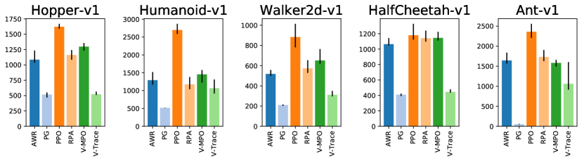
Figure 1: Comparison of different policy losses (CB.3).

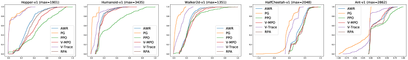
Figure 4: Empirical cumulative density functions of agent performance conditioned on different values of Policy loss (CB.3). The x axis denotes performance rescaled so that 0 corresponds to a random policy and 1 to the best found configuration, and the y axis denotes the quantile.

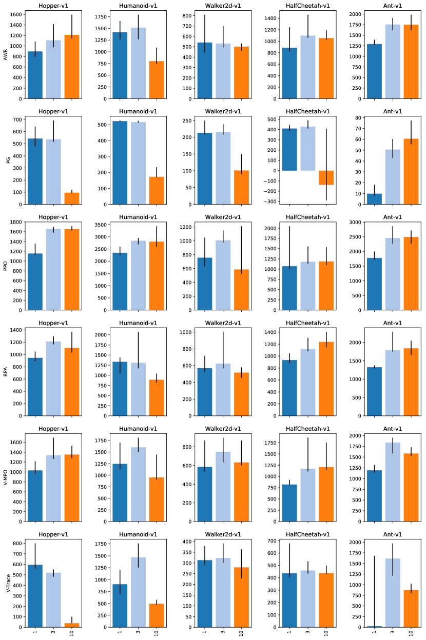
Figure 14: 95th percentile of performance scores conditioned on Policy loss (CB.3)(rows) and num_epochs (CB.1)(bars).

Interpretation. Fig. 1 shows the 95-th percentile of the average policy score during training for different policy losses (CB.3). We observe that PPO performs better than the other losses on 4 out of 5 environments and is one of the top performing losses on HalfCheetah. As we randomly sample the loss specific hyperparameters in this analysis, one might argue that our approach favours choices that are not too sensitive to hyperparameters. At the same time, there might be losses that are sensitive to their hyperparameters but for which good settings may be easily found. Fig. 5 shows that even if we condition on choosing the optimal loss hyperparameters for each loss, PPO still outperforms the other losses on the two hardest tasks — Humanoid and Ant and is one of the top performing losses on the other $3$ tasks. Moreover, we show the empirical cumulative density functions of agent performance conditioned on the policy loss used in Fig. 4. Perhaps unsurprisingly, PG and V-trace perform worse on all tasks. This is likely caused by their inability to handle data that become off-policy in one iteration, either due to multiple passes (CB.1) over experience (which can be seen in Fig. 14) or a large experience buffer (CB.1) in relation to the batch size (CB.1). Overall, these results show that trust-region optimization (preventing the current policy from diverging too much from the behavioral one) which is present in all the other policy losses is crucial for good sample complexity. For PPO and its clipping threshold $\epsilon$ (C• ‣ B.3), we further observe that $\epsilon=0.2$ and $\epsilon=0.3$ perform reasonably well in all environments but that lower ($\epsilon=0.1$) or higher ($\epsilon=0.5$) values give better performance on some of the environments (See Fig. 10 and Fig. 32).

Recommendation. Use the PPO policy loss. Start with the clipping threshold set to $0.25$ but also try lower and higher values if possible.

3.2 Networks architecture (based on the results in Appendix E)

Study description. We investigate the impact of differences in the policy and value function neural network architectures. We consider choices related to the network structure and size (CB.7, CB.7, CB.7, CB.7, CB.7, CB.7, CB.7), activation functions (CB.7), and initialization of network weights (CB.7, CB.7, CB.7). We further include choices related to the standard deviation of actions (C• ‣ B.8, C• ‣ B.8, C• ‣ B.8, C• ‣ B.8) and transformations of sampled actions (C• ‣ B.8).

Interpretation. Separate value and policy networks (CB.7) appear to lead to better performance on four out of five environments (Fig. 15). To avoid analyzing the other choices based on bad models, we thus focus for the rest of this experiment only on agents with separate value and policy networks. Regarding network sizes, the optimal width of the policy MLP depends on the complexity of the environment (Fig. 18) and too low or too high values can cause significant drop in performance while for the value function there seems to be no downside in using wider networks (Fig. 21). Moreover, on some environments it is beneficial to make the value network wider than the policy one, e.g. on HalfCheetah the best results are achieved with $16-32$ units per layer in the policy network and $256$ in the value network. Two hidden layers appear to work well for policy (Fig. 22) and value networks (Fig. 20) in all tested environments. As for activation functions, we observe that tanh activations perform best and relu worst. (Fig. 30).

Interestingly, the initial policy appears to have a surprisingly high impact on the training performance. The key recipe appears is to initialize the policy at the beginning of training so that the action distribution is centered around $0$ regardless of the observation and has a rather small standard deviation. This can be achieved by initializing the policy MLP with smaller weights in the last layer (CB.7, Fig. 24, this alone boosts the performance on Humanoid by 66%) so that the initial action distribution is almost independent of the observation and by introducing an offset in the standard deviation of actions (C• ‣ B.8). Fig. 2 shows that the performance is very sensitive to the initial action standard deviation with 0.5 performing best on all environments except Hopper where higher values perform better.

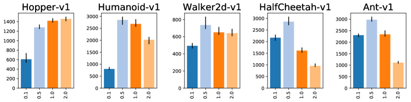
Figure 2: Comparison of different initial standard deviations of actions (C• ‣ B.8).

Fig. 17 compares two approaches to transform unbounded sampled actions into the bounded $[-1,\,1]$ domain expected by the environment (C• ‣ B.8): clipping and applying a tanh function. tanh performs slightly better overall (in particular it improves the performance on HalfCheetah by $30\%$ ). Comparing Fig. 17 and Fig. 2 suggests that the difference might be mostly caused by the decreased magnitude of initial actions.

Other choices appear to be less important: The scale of the last layer initialization matters much less for the value MLP (CB.7) than for the policy MLP (Fig. 19). Apart from the last layer scaling, the network initialization scheme (CB.7) does not matter too much (Fig. 27). Only he_normal and he_uniform [7] appear to be suboptimal choices with the other options performing very similarly. There also appears to be no clear benefits if the standard deviation of the policy is learned for each state (i.e. outputted by the policy network) or once globally for all states (C• ‣ B.8, Fig. 23). For the transformation of policy output into action standard deviation (C• ‣ B.8), softplus and exponentiation perform very similarly (Fig. 25). Finally, the minimum action standard deviation (C• ‣ B.8) seems to matter little, if it is not set too large (Fig. 30).

Recommendation. Initialize the last policy layer with $100\times$ smaller weights. Use softplus to transform network output into action standard deviation and add a (negative) offset to its input to decrease the initial standard deviation of actions. Tune this offset if possible. Use tanh both as the activation function (if the networks are not too deep) and to transform the samples from the normal distribution to the bounded action space. Use a wide value MLP (no layers shared with the policy) but tune the policy width (it might need to be narrower than the value MLP).

3.3 Normalization and clipping (based on the results in Appendix F)

Study description. We investigate the impact of different normalization techniques: observation normalization (C• ‣ B.9), value function normalization (C• ‣ B.9), per-minibatch advantage normalization (C• ‣ B.9), as well as gradient (C• ‣ B.9) and observation (C• ‣ B.9) clipping.

Interpretation. Input normalization (C• ‣ B.9) is crucial for good performance on all environments apart from Hopper (Fig. 33). Quite surprisingly, value function normalization (C• ‣ B.9) also influences the performance very strongly — it is crucial for good performance on HalfCheetah and Humanoid, helps slightly on Hopper and Ant and significantly hurts the performance on Walker2d (Fig. 37). We are not sure why the value function scale matters that much but suspect that it affects the performance by changing the speed of the value function fitting. In contrast to observation and value function normalization, per-minibatch advantage normalization (C• ‣ B.9) seems not to affect the performance too much (Fig. 35). Similarly, we have found little evidence that clipping normalized observations (C• ‣ B.9) helps (Fig. 38) but it might be worth using if there is a risk of extremely high observations due to simulator divergence. Finally, gradient clipping (C• ‣ B.9) provides a small performance boost with the exact clipping threshold making little difference (Fig. 34).

Recommendation. Always use observation normalization and check if value function normalization improves performance. Gradient clipping might slightly help but is of secondary importance.

3.4 Advantage Estimation (based on the results in Appendix G)

Study description. We compare the most commonly used advantage estimators (CB.2): N-step [3], GAE [9] and V-trace [19] and their hyperparameters (C• ‣ B.2, C• ‣ B.2, C• ‣ B.2, C• ‣ B.2). We also experiment with applying PPO-style pessimistic clipping (CB.2) to the value loss (present in the original PPO implementation but not mentioned in the PPO paper [17]) and using Huber loss [1] instead of MSE for value learning (CB.2, CB.2). Moreover, we varied the number of parallel environments used (CB.1) as it changes the length of the experience fragments collected in each step.

Interpretation. GAE and V-trace appear to perform better than N-step returns (Fig. 44 and 40) which indicates that it is beneficial to combine the value estimators from multiple timesteps. We have not found a significant performance difference between GAE and V-trace in our experiments. $\lambda=0.9$ (C• ‣ B.2, C• ‣ B.2) performed well regardless of whether GAE (Fig. 45) or V-trace (Fig. 49) was used on all tasks but tuning this value per environment may lead to modest performance gains. We have found that PPO-style value loss clipping (CB.2) hurts the performance regardless of the clipping threshold (Fig. 43). Similarly, the Huber loss (CB.2) performed worse than MSE in all environments (Fig. 42) regardless of the value of the threshold (CB.2) used (Fig. 48).

Recommendation. Use GAE with $\lambda=0.9$ but neither Huber loss nor PPO-style value loss clipping.

3.5 Training setup (based on the results in Appendix H)

Study description. We investigate choices related to the data collection and minibatch handling: the number of parallel environments used (CB.1), the number of transitions gathered in each iteration (CB.1), the number of passes over the data (CB.1), minibatch size (CB.1) and how the data is split into minibatches (CB.1).

For the last choice, in addition to standard choices, we also consider a new small modification of the original PPO approach: The original PPO implementation splits the data in each policy iteration step into individual transitions and then randomly assigns them to minibatches (CB.1). This makes it impossible to compute advantages as the temporal structure is broken. Therefore, the advantages are computed once at the beginning of each policy iteration step and then used in minibatch policy and value function optimization. This results in higher diversity of data in each minibatch at the cost of using slightly stale advantage estimations. As a remedy to this problem, we propose to recompute the advantages at the beginning of each pass over the data instead of just once per iteration.

Results. Unsurprisingly, going over the experience multiple times appears to be crucial for good sample complexity (Fig. 54). Often, this is computationally cheap due to the simple models considered, in particular on machines with accelerators such as GPUs and TPUs. As we increase the number of parallel environments (CB.1), performance decreases sharply on some of the environments (Fig. 55). This is likely caused by shortened experience chunks (See Sec. B.1 for the detailed description of the data collection process) and earlier value bootstrapping. Despite that, training with more environments usually leads to faster training in wall-clock time if enough CPU cores are available. Increasing the batch size (CB.1) does not appear to hurt the sample complexity in the range we tested (Fig. 57) which suggests that it should be increased for faster iteration speed. On the other hand, the number of transitions gathered in each iteration (CB.1) influences the performance quite significantly (Fig. 52). Finally, we compare different ways to handle minibatches (See Sec. B.1 for the detailed description of different variants) in Fig. 53 and  58. The plots suggest that stale advantages can in fact hurt performance and that recomputing them at the beginning of each pass at least partially mitigates the problem and performs best among all variants.

Recommendation. Go over experience multiple times. Shuffle individual transitions before assigning them to minibatches and recompute advantages once per data pass (See App. B.1 for the details). For faster wall-clock time training use many parallel environments and increase the batch size (both might hurt the sample complexity). Tune the number of transitions in each iteration (CB.1) if possible.

3.6 Timesteps handling (based on the results in Appendix I)

Study description. We investigate choices related to the handling of timesteps: discount factor (CB.4), frame skip (CB.4), and how episode termination due to timestep limits are handled (CB.4). The latter relates to a technical difficulty explained in App. B.4 where one assumes for the algorithm an infinite time horizon but then trains using a finite time horizon [16].

Interpretation. Fig. 60 shows that the performance depends heavily on the discount factor $\gamma$ (CB.4) with $\gamma=0.99$ performing reasonably well in all environments. Skipping every other frame (CB.4) improves the performance on $2$ out of $5$ environments (Fig. 61). Proper handling of episodes abandoned due to the timestep limit seems not to affect the performance (CB.4, Fig. 62) which is probably caused by the fact that the timestep limit is quite high ($1000$ transitions) in all the environments we considered.

Recommendation. Discount factor $\gamma$ is one of the most important hyperparameters and should be tuned per environment (start with $\gamma=0.99$). Try frame skip if possible. There is no need to handle environments step limits in a special way for large step limits.

3.7 Optimizers (based on the results in Appendix J)

Study description. We investigate two gradient-based optimizers commonly used in RL: (CB.5) – Adam [8] and RMSprop – as well as their hyperparameters (CB.5, CB.5, CB.5, CB.5, CB.5, CB.5, CB.5) and a linear learning rate decay schedule (CB.5).

Interpretation. The differences in performance between the optimizers (CB.5) appear to be rather small with no optimizer consistently outperforming the other across environments (Fig. 66). Unsurprisingly, the learning rate influences the performance very strongly (Fig. 69) with the default value of $0.0003$ for Adam (CB.5) performing well on all tasks. Fig. 67 shows that Adam works better with momentum (CB.5). For RMSprop, momentum (CB.5) makes less difference (Fig. 71) but our results suggest that it might slightly improve performance. Whether the centered or uncentered version of RMSprop is used (CB.5) makes no difference (Fig. 70) and similarly we did not find any difference between different values of the $\epsilon$ coefficients (CB.5, CB.5, Fig. 68 and 72). Linearly decaying the learning rate to $0$ increases the performance on $4$ out of $5$ tasks but the gains are very small apart from Ant, where it leads to $15\%$ higher scores (Fig. 65).

Recommendation. Use Adam [8] optimizer with momentum $\beta_{1}=0.9$ and a tuned learning rate ($0.0003$ is a safe default). Linearly decaying the learning rate may slightly improve performance but is of secondary importance.

3.8 Regularization (based on the results in Appendix K)

Study description. We investigate different policy regularizers (CB.6), which can have either the form of a penalty (CB.6, e.g. bonus for higher entropy) or a soft constraint (CB.6, e.g. entropy should not be lower than some threshold) which is enforced with a Lagrange multiplier. In particular, we consider the following regularization terms: entropy (C1, C1), the Kullback–Leibler divergence (KL) between a reference $\mathcal{N}(0,1)$ action distribution and the current policy (C1, C1) and the KL divergence and reverse KL divergence between the current policy and the behavioral one (C1, C1, C1, C1), as well as the “decoupled” KL divergence from [18, 34] (C1, C1, C1, C1).

Interpretation. We do not find evidence that any of the investigated regularizers helps significantly on our environments with the exception of HalfCheetah on which all constraints (especially the entropy constraint) help (Fig. 76 and 77). However, the performance boost is largely independent on the constraint threshold (Fig. 83, 84, 87, 89, 90 and 91) which suggests that the effect is caused by the initial high strength of the penalty (before it gets adjusted) and not by the desired constraint. While it is a bit surprising that regularization does not help at all (apart from HalfCheetah), we conjecture that regularization might be less important in our experiments because: (1) the PPO policy loss already enforces the trust region which makes KL penalties or constraints redundant; and (2) the careful policy initialization (See Sec. 3.2) is enough to guarantee good exploration and makes the entropy bonus or constraint redundant.

4 Related Work

Islam et al. [15] and Henderson et al. [22] point out the reproducibility issues in RL including the performance differences between different code bases, the importance of hyperparameter tuning and the high level of stochasticity due to random seeds. Tucker et al. [26] showed that the gains, which had been attributed to one of the recently proposed policy gradients improvements, were, in fact, caused by the implementation details. The most closely related work to ours is probably Engstrom et al. [27] where the authors investigate code-level improvements in the PPO [17] code base and conclude that they are responsible for the most of the performance difference between PPO and TRPO [10]. Our work is also similar to other large-scale studies done in other fields of Deep Learning, e.g. model-based RL [31], GANs [24], NLP [35], disentangled representations [23] and convolution network architectures [36].

5 Conclusions

In this paper, we investigated the importance of a broad set of high- and low-level choices that need to be made when designing and implementing on-policy learning algorithms. Based on more than 250’000 experiments in five continuous control environments, we evaluate the impact of different choices and provide practical recommendations. One of the surprising insights is that the initial action distribution plays an important role in agent performance. We expect this to be a fruitful avenue for future research.

Appendix A Reinforcement Learning Background

We consider the standard reinforcement learning formalism consisting of an agent interacting with an environment. To simplify the exposition we assume in this section that the environment is fully observable. An environment is described by a set of states $\mathcal{S}$, a set of actions $\mathcal{A}$, a distribution of initial states $p(s_{0})$, a reward function $r:\mathcal{S}\times\mathcal{A}\rightarrow\mathbb{R}$, transition probabilities $p(s_{t+1}|s_{t},a_{t})$ ($t$ is a timestep index explained later), termination probabilities $T(s_{t},a_{t})$ and a discount factor $\gamma\in[0,1]$.

A policy $\pi$ is a mapping from state to a distribution over actions. Every episode starts by sampling an initial state $s_{0}$. At every timestep $t$ the agent produces an action based on the current state: $a_{t}\sim\pi(\cdot|s_{t})$. In turn, the agent receives a reward $r_{t}=r(s_{t},a_{t})$ and the environment’s state is updated. With probability $T(s_{t},a_{t})$ the episode is terminated, and otherwise the new environments state $s_{t+1}$ is sampled from $p(\cdot|s_{t},a_{t})$. The discounted sum of future rewards, also referred to as the return, is defined as $R_{t}=\sum_{i=t}^{\infty}\gamma^{i-t}r_{i}$. The agent’s goal is to find the policy $\pi$ which maximizes the expected return $\mathbb{E}_{\pi}[R_{0}|s_{0}]$, where the expectation is taken over the initial state distribution, the policy, and environment transitions accordingly to the dynamics specified above. The Q-function or action-value function of a given policy $\pi$ is defined as $Q^{\pi}(s_{t},a_{t})=\mathbb{E}_{\pi}[R_{t}|s_{t},a_{t}]$, while the V-function or state-value function is defined as $V^{\pi}(s_{t})=\mathbb{E}_{\pi}[R_{t}|s_{t}]$. The value $A^{\pi}(s_{t},a_{t})=Q^{\pi}(s_{t},a_{t})-V^{\pi}(s_{t})$ is called the advantage and tells whether the action $a_{t}$ is better or worse than an average action the policy $\pi$ takes in the state $s_{t}$.

In practice, the policies and value functions are going to be represented as neural networks. In particular, RL algorithms we consider maintain two neural networks: one representing the current policy $\pi$ and a value network which approximates the value function of the current policy $V\approx V^{\pi}$.

Appendix B List of Investigated Choices

In this section we list all algorithmic choices which we consider in our experiments. See Sec. A for a very brief introduction to RL and the notation we use in this section.

B.1 Data collection and optimization loop

RL algorithms interleave running the current policy in the environment with policy and value function networks optimization. In particular, we create num_envs (CB.1) environments [14]. In each iteration, we run all environments synchronously sampling actions from the current policy until we have gathered iteration_size (CB.1) transitions total (this means that we have num_envs (CB.1) experience fragments, each consisting of $\texttt{iteration\_size{ }(C\ref{choice:stepsize})}~{}/~{}\texttt{num\_envs{ }(C\ref{choice:numenvs})}$ transitions). Then, we perform num_epochs (CB.1) epochs of minibatch updates where in each epoch we split the data into minibatches of size batch_size (CB.1), and performing gradient-based optimization [17]. Going over collected experience multiple times means that it is not strictly an on-policy RL algorithm but it may increase the sample complexity of the algorithm at the cost of more computationally expensive optimization step.

We consider four different variants of the above scheme (choice CB.1):

• Fixed trajectories: Each minibatch consists of full experience fragments and in each epoch we go over exactly the same minibatches in the same order.

• Shuffle trajectories: Like Fixed trajectories but we randomly assign full experience fragments to minibatches in each epoch.

• Shuffle transitions: We break experience fragments into individual transitions and assign them randomly to minibatches in each epoch. This makes the estimation of advantages impossible in each minibatch (most of the advantage estimators use future states, See App. B.2) so we precompute all advantages at the beginning of each iteration using full experience fragments. This approach leads to higher diversity of data in each minibatch at the price of somewhat stale advantage estimations. The original PPO implementation from OpenAI Baselines works this way but this is not mentioned in the PPO paper [17].

• Shuffle transitions (recompute advantages): Like Shuffle transitions but we recompute advantages at the beginning of each epoch.

B.2 Advantage estimation

Let $V$ be an approximator of the value function of some policy, i.e. $V\approx V^{\pi}$. We experimented with the three most commonly used advantage estimators in on-policy RL (choice CB.2):

• N-step return [3] is defined as

  $$\hat{V}_{t}^{(N)}=\sum_{i=t}^{t+N-1}\gamma^{i-t}r_{i}+\gamma^{N}V(s_{t+N})\approx V^{\pi}(s_{t}).$$

  The parameter $N$ (choice C• ‣ B.2) controls the bias–variance tradeoff of the estimator with bigger values resulting in an estimator closer to empirical returns and having less bias and more variance. Given N-step returns we can estimate advantages as follows:

  $$\hat{A}_{t}^{\text{(N)}}=\hat{V}_{t}^{\text{(N)}}-V(s_{t})\approx A^{\pi}(s_{t},a_{t}).$$

• Generalized Advantage Estimator, GAE($\lambda$) [9] is a method that combines multi-step returns in the following way:

  $$\hat{V}_{t}^{\text{GAE}}=(1-\lambda)\sum_{N>0}\lambda^{N-1}\hat{V}_{t}^{(N)}\approx V^{\pi}(s_{t}),$$

  where $0<\lambda<1$ is a hyperparameter (choice C• ‣ B.2) controlling the bias–variance trade-off. Using this, we can estimate advantages with:

  $$\hat{A}_{t}^{\text{GAE}}=\hat{V}_{t}^{\text{GAE}}-V(s_{t})\approx A^{\pi}(s_{t},a_{t}).$$

  It is possible to compute the values of this estimator for all states encountered in an episode in linear time [9].

• V-trace($\lambda,\bar{c},\bar{\rho}$) [19] is an extension of GAE which introduces truncated importance sampling weights to account for the fact that the current policy might be slightly different from the policy which generated the experience. It is parameterized by $\lambda$ (choice C• ‣ B.2) which serves the same role as in GAE and two parameters $\bar{c}$ and $\bar{\rho}$ which are truncation thresholds for two different types of importance weights. See [19] for the detailed description of the V-trace estimator. All experiments in the original paper [19] use $\bar{c}=\bar{\rho}=1$. Similarly, we only consider the case $\bar{c}=\bar{\rho}$, i.e., we consider a single choice V-Trace advantage $c,\,\rho$ (C• ‣ B.2).

The value network is trained by fitting one of the returns described above with an MSE (quadratic) or a Huber [1] loss (choice CB.2). Huber loss is a quadratic around zero up to some threshold (choice CB.2) at which point it becomes a linear function.

The original PPO implementation [17] uses an additional pessimistic clipping in the value loss function. See [27] for the description of this technique. It is parameterized by a clipping threshold (choice CB.2).

B.3 Policy losses

Let $\pi$ denote the policy being optimized, and $\mu$ the behavioral policy, i.e. the policy which generated the experience. Moreover, let $\hat{A}_{t}^{\pi}$ and $\hat{A_{t}^{\mu}}$ be some estimators of the advantage at timestep $t$ for the policies $\pi$ and $\mu$.

We consider optimizing the policy with the following policy losses (choice CB.3):

• Policy Gradients (PG) [2] with advantages: $\mathcal{L}_{\texttt{PG}}=-\log\pi(a_{t}|s_{t})\hat{A}_{t}^{\pi}$. It can be shown that if $\hat{A}_{t}^{\pi}$ estimators are unbiased, then $\nabla_{\theta}\mathcal{L}_{\texttt{PG}}$ is an unbiased estimator of the gradient of the policy performance assuming that experience was generated by the current policy $\pi$.

• V-trace [19]: $\mathcal{L}_{\texttt{V-trace}}^{\bar{\rho}}=\textbf{sg}(\rho_{t})\mathcal{L}_{\texttt{PG}},$ where $\rho_{t}=\min(\frac{\pi(a_{t}|s_{t})}{\mu(a_{t}|s_{t})},\bar{\rho})$ is a truncated importance weight, sg is the stop_gradient operator and $\bar{\rho}$ is a hyperparameter (choice C• ‣ B.3). $\nabla_{\theta}L_{\texttt{V-trace}}^{\bar{\rho}}$ is an unbiased estimator of the gradient of the policy performance if $\bar{\rho}=\infty$ regardless of the behavioural policy$\mu$.

• Proximal Policy Optimization (PPO) [17]:

  $$\mathcal{L}^{\epsilon}_{\text{PPO}}=-\min\left[\frac{\pi(a_{t}|s_{t})}{\mu(a_{t}|s_{t})}\hat{A}_{t}^{\pi},\,\mbox{clip}\left(\frac{\pi(a_{t}|s_{t})}{\mu(a_{t}|s_{t})},\,\frac{1}{1+\epsilon},\,1+\epsilon\right)\hat{A}_{t}^{\pi}\right],$$

  where $\epsilon$ is a hyperparameter C• ‣ B.3. This loss encourages the policy to take actions which are better than average (have positive advantage) while clipping discourages bigger changes to the policy by limiting how much can be gained by changing the policy on a particular data point.

• Advantage-Weighted Regression (AWR) [33]:

  $$\mathcal{L}_{\texttt{AWR}}^{\beta,\,\omega_{\texttt{max}}}=-\log\pi(a_{t}|s_{t})\min\left(\exp(A_{t}^{\mu}/\beta),\,\omega_{\texttt{max}}\right).$$

  It can be shown that for $\omega_{\texttt{max}}=\infty$ (choice C• ‣ B.3) it corresponds to an approximate optimization of the policy $\pi$ under a constraint of the form $\texttt{KL}(\pi||\mu)<\epsilon$ where the KL bound $\epsilon$ depends on the exponentiation temperature $\beta$ (choice C• ‣ B.3). Notice that in contrast to previous policy losses, AWR uses estimates of the advantages for the behavioral policy ($A_{t}^{\mu}$) and not the current one ($A_{t}^{\pi}$). AWR was proposed mostly as an off-policy RL algorithm.

• On-Policy Maximum a Posteriori Policy Optimization (V-MPO) [34]: This policy loss is the same as AWR with the following differences: (1) exponentiation is replaced with the softmax operator and there is no clipping with $\omega_{\texttt{max}}$; (2) only samples with the top half advantages in each batch are used; (3) the temperature $\beta$ is treated as a Lagrange multiplier and adjusted automatically to keep a constraint on how much the weights (i.e. softmax outputs) diverge from a uniform distribution with the constraint threshold $\epsilon$ being a hyperparameter (choice C• ‣ B.3). (4) A soft constraint on $\texttt{KL}(\mu||\pi)$ is added. In our experiments, we did not treat this constraint as a part of the V-MPO policy loss as policy regularization is considered separately (See Sec. B.6).

• Repeat Positive Advantages (RPA): $\mathcal{L}_{\texttt{RPA}}=-\log\pi(a_{t}|s_{t})[A_{t}>0]$. This is a new loss we introduce in this paper. We choose this loss because it is the limiting case of AWR and V-MPO. In particular, $\mathcal{L}_{\texttt{AWR}}^{\beta,\,\omega_{\texttt{max}}}$ converges to $\omega_{\texttt{max}}\mathcal{L}_{\texttt{RPA}}$ for $\beta\rightarrow 0$ and for $\epsilon\rightarrow 0$ V-MPO converges to RPA with $[A_{t}>0]$ replaced by only taking the top half advantages in each batch (the two conditions become even more similar if advantage normalization is used, See Sec. B.9).

B.4 Handling of timesteps

The most important hyperparameter controlling how timesteps are handled is the discount factor $\gamma$ (choice CB.4). Moreover, we consider the so-called frame skip (choice CB.4). Frame skip equal to $n$ means that we modify the environment by repeating each action outputted by the policy $n$ times (unless the episode has terminated in the meantime) and sum the received rewards. When using frame skip, we also adjust the discount factor appropriately, i.e. we discount with $\gamma^{n}$ instead of $\gamma$.

Many reinforcement learning environments (including the ones we use in our experiments) have step limits which means that an episode is terminated after some fixed number of steps (assuming it was not terminated earlier for some other reason). Moreover, the number of remaining environment steps is not included in policy observations which makes the environments non-Markovian and can potentially make learning harder [16]. We consider two ways to handle such abandoned episodes. We either treat the final transition as any other terminal transition, e.g. the value target for the last state is equal to the final reward, or we take the fact that we do not know what would happen if the episode was not terminated into account. In the latter case, we set the advantage for the final state to zero and its value target to the current value function. This also influences the value targets for prior states as the value targets are computed recursively [9, 19]. We denote this choice by Handle abandoned? (CB.4).

B.5 Optimizers

We experiment with two most commonly used gradient-based optimizers in RL (choice CB.5): Adam [8] and RMSProp. You can find the description of the optimizers and their hyperparameters in the original publications. For both optimizers, we sweep the learning rate (choices CB.5 and CB.5), momentum (choices CB.5 and CB.5) and the $\epsilon$ parameters added for numerical stability (choice CB.5 and CB.5). Moreover, for RMSProp we consider both centered and uncentered versions (choice CB.5). For their remaining hyperparameters, we use the default values from TensorFlow [11], i.e. $\beta_{2}=0.999$ for Adam and $\rho=0.1$ for RMSProp. Finally, we allow a linear learning rate schedule via the hyperparameter Learning rate decay (CB.5) which defines the terminal learning rate as a fraction of the initial learning rate (i.e., $0.0$ correspond to a decay to zero whereas $1.0$ corresponds to no decay).

B.6 Policy regularization

We consider three different modes for regularization (choice CB.6):

• No regularization: We apply no regularization.

• Penalty: we apply a regularizer $R$ with fixed strength, i.e., we add to the loss the term $\alpha R$ for some fixed coefficient $\alpha$ which is a hyperparameter.

• Constraint: We impose a soft constraint of the form $R<\epsilon$ on the value of the regularizer where $\epsilon$ is a hyperparameter. This can be achieved by treating $\alpha$ as a Lagrange multiplier. In this case, we optimize the value of $\alpha>0$ together with the networks parameter by adding to the loss the term $\alpha\cdot\textbf{sg}(\epsilon-R)$, where sg in the stop_gradient operator. In practice, we use the following parametrization $\alpha=\exp(c\cdot p)$ where $p$ is a trainable parameter (initialized with $0$) and $c$ is a coefficient controlling how fast $\alpha$ is adjusted (we use $c=10$ in all experiments). After each gradient step, we clip the value of $p$ to the range $[\log(10^{-6})/10,\,\log(10^{6})/10]$ to avoid extremely small and large values.

We consider a number of different policy regularizers both for penalty (choice CB.6) and constraint regularization (choice CB.6):

• Entropy $\texttt{H}(\pi(\cdot|s))$ — it encourages the policy to try diverse actions [4].

• $\texttt{KL}(\mu(\cdot|s)||\pi(\cdot|s))$ — the Kullback–Leibler divergence between the behavioral and the current policy [10] prevents the probability of taking a given action from decreasing too rapidly.

• $\texttt{KL}(\pi(\cdot|s)||\mu(\cdot|s))$ — similar to the previous one but prevents too rapid increase of probabilities.

• $\texttt{KL}(\texttt{ref}(\cdot|s)||\pi(\cdot|s))$ where ref is some reference distribution. We use $\texttt{ref}=\mathcal{N}(0,1)$ in all experiments. This kind of regularization encourages the policy to try all possible actions.

• Decoupled $\texttt{KL}(\mu(\cdot|s)||\pi(\cdot|s))$. For Gaussian distributions we can split $\texttt{KL}(\mu(\cdot|s)||\pi(\cdot|s))$ into a term which depends on the change in the mean of the distribution and another one which depends on the change in the standard deviation: $\texttt{KL}(\mu(\cdot|s)||\pi(\cdot|s))=\texttt{KL}(\mu(\cdot|s)||\zeta(\cdot|s))+\texttt{KL}(\zeta(\cdot|s)||\pi(\cdot|s))$ where $\zeta(\cdot|s)$ is a Gaussian distribution with same mean as $\mu(\cdot|s)$ and the same standard deviation as $\pi(\cdot|s)$. Therefore, instead of using $\texttt{KL}(\mu(\cdot|s)||\pi(\cdot|s))$ directly, we can use two separate regularizers, $\texttt{KL}(\mu(\cdot|s)||\zeta(\cdot|s))$ and $\texttt{KL}(\zeta(\cdot|s)||\pi(\cdot|s))$, with different strengths. The soft constraint version of this regularizer in used in V-MPO [34] with the threshold on $\texttt{KL}(\mu(\cdot|s)||\zeta(\cdot|s))$ being orders of magnitude lower than the one on $\texttt{KL}(\zeta(\cdot|s)||\pi(\cdot|s))$.

While one could add any linear combination of the above terms to the loss, we have decided to only use a single regularizer in each experiment. Overall, all these combinations of regularization modes and different hyperparameters lead to the choices detailed in Table 1.

Table 1: Choices pertaining to regularization.

Choice	Name
CB.6	Regularization type
CB.6	Regularizer (in case of penalty)
CB.6	Regularizer (in case of constraint)
C1	Threshold for $\texttt{KL}(\mu||\pi)$
C1	Threshold for $\texttt{KL}(\pi||\mu)$
C1	Threshold for $\texttt{KL}(\texttt{ref}||\pi)$
C1	Threshold for mean in decoupled $\texttt{KL}(\mu||\pi)$
C1	Threshold for std in decoupled $\texttt{KL}(\mu||\pi)$
C1	Threshold for entropy $H(\pi)$
C1	Regularizer coefficient for $\texttt{KL}(\mu||\pi)$
C1	Regularizer coefficient for $\texttt{KL}(\pi||\mu)$
C1	Regularizer coefficient for $\texttt{KL}(\texttt{ref}||\pi)$
C1	Regularizer coefficient for mean in decoupled $\texttt{KL}(\mu||\pi)$
C1	Regularizer coefficient for std in decoupled $\texttt{KL}(\mu||\pi)$
C1	Regularizer coefficient for entropy

B.7 Neural network architecture

We use multilayer perceptrons (MLPs) to represent policies and value functions. We either use separate networks for the policy and value function, or use a single network with two linear heads, one for the policy and one for the value function (choice CB.7). We consider different widths for the shared MLP (choice CB.7), the policy MLP (choice CB.7) and the value MLP (choice CB.7) as well as different depths for the shared MLP (choice CB.7), the policy MLP (choice CB.7) and the value MLP (choice CB.7). If we use the shared MLP, we further add a hyperparameter Baseline cost (shared) (CB.7) that rescales the contribution of the value loss to the full objective function. This is important in this case as the shared layers of the MLP affect the loss terms related to both the policy and the value function. We further consider different activation functions (choice CB.7) and different neural network initializers (choice CB.7). For the initialization of both the last layer in the policy MLP / the policy head (choice CB.7) and the last layer in the value MLP / the value head (choice CB.7), we further consider a hyperparameter that rescales the network weights of these layers after initialization.

B.8 Action distribution parameterization

A policy is a mapping from states to distributions of actions. In practice, a parametric distribution is chosen and the policy output is treated as the distribution parameters. The vast majority of RL applications in continuous control use a Gaussian distribution to represent the action distribution and this is also the approach we take.

This, however, still leaves a few decisions which need to be make in the implementation:

• Should the standard deviation of actions be a part of the network output (used e.g. in [21]) or should it be independent of inputs like in [17] (choice C• ‣ B.8)? In the latter case, the standard deviation is still learnable but it is the same for each state.

• Gaussian distributions are parameterized with a mean and a standard deviation which has to be non-negative. What function should be used to transform network outputs which can be negative into the standard deviation (choice C• ‣ B.8)? We consider exponentiation (used e.g. in [17]) and the softplus function (used e.g. in [29]).

• What should be the initial standard deviation of the action distribution (choice C• ‣ B.8)? We can control it by adding some fixed value to the input to the function computing the standard deviation (e.g. softplus).

• Should we add a small value to the standard deviation to avoid very low values (choice C• ‣ B.8)?

• Most continuous control environments expect actions from a bounded range (often $[-1,\,1]$) but the commonly used Gaussian distribution can produce values of an arbitrary magnitude. We consider two approaches to handle this (choice C• ‣ B.8): The easiest solution is to just clip the action to the allowed range when sending it to the environment (used e.g. in [17]). Another approach is to apply the tanh function to the distribution to bound the range of actions (used e.g. in [25]). This additional transformation changes the density of actions — if action $u$ is parameterized as $u=\texttt{tanh}(x)$, where $x$ is a sample from a Gaussian distribution with probability density function $p_{\theta}$, than the density of $u$ is $\log p_{u}(u)=\log p_{\theta}(x)-\log\tanh^{\prime}(x)$, where $x=\tanh^{-1}(u)$. This additional $\log\tanh^{\prime}(x)$ term does not affect policy losses because they only use $\nabla_{\theta}\log p_{u}(u)=\nabla_{\theta}\log p_{\theta}(x)$. Similarly, this term does not affect the KL divergences which may be used for regularization (See Sec. B.6) because the KL divergence has a form of the difference of two log-probabilities on the same sample and the two $\log\tanh^{\prime}(x)$ terms cancel out. The only place where the $\log\tanh^{\prime}(x)$ term affects the policy gradient computation and should be included is the entropy regularization as $H(U)=-\mathbb{E}_{u}\log p_{u}(u)=\mathbb{E}_{x}[-\log p_{\theta}(x)+\log\tanh^{\prime}(x)]$. This additional $\log\tanh^{\prime}(x)$ term penalizies the policy for taking extreme actions which prevents $\tanh$ saturation and the loss of the gradient. Moreover, it prevents the action entropy from becoming unbounded.

To sum up, we parameterize the actions distribution as

$$T_{u}(\mathcal{N}(x_{\mu},\,T_{\rho}(x_{\rho}+c_{\rho})+\epsilon_{\rho})),$$

where

• $x_{\mu}$ is a part of the policy network output,

• $x_{\rho}$ is either a part of the policy network output or a separate learnable parameter (one per action dimension),

• $\epsilon_{\rho}$ (C• ‣ B.8) is a hyperparameter controlling minimal standard deviation,

• $T_{\rho}$ (C• ‣ B.8) is a standard deviation transformation ($\mathbb{R}\rightarrow\mathbb{R}_{\geq 0}$),

• $T_{u}$ (C• ‣ B.8) is an action transformation ($\mathbb{R}\rightarrow[-1,\,1]$),

• $c_{\rho}$ is a constant controlling the initial standard deviation and computed as $c_{\rho}=T_{\rho}^{-1}(i_{\rho}-\epsilon_{\rho})$ where $i_{\rho}$ is the desired initial standard deviation (C• ‣ B.8).

B.9 Data normalization and clipping

While it is not always mentioned in RL publications, many RL implementations perform different types of data normalization. In particular, we consider the following:

• Observation normalization (choice C• ‣ B.9). If enabled, we keep the empirical mean $o_{\mu}$ and standard deviation $o_{\rho}$ of each observation coordinate (based on all observations seen so far) and normalize observations by subtracting the empirical mean and dividing by $\max(o_{\rho},\,10^{-6})$. This results in all neural networks inputs having approximately zero mean and standard deviation equal to one. Moreover, we optionally clip the normalized observations to the range $[-o_{\texttt{max}},\,o_{\texttt{max}}]$ where $o_{\texttt{max}}$ is a hyperparameter (choice C• ‣ B.9).

• Value function normalization (choice C• ‣ B.9). Similarly to observations, we also maintain the empirical mean $v_{\mu}$ and standard deviation $v_{\rho}$ of value function targets (See Sec. B.2). The value function network predicts normalized targets $(\hat{V}-v_{\mu})/\max(v_{\rho},\,10^{-6})$ and its outputs are denormalized accordingly to obtain predicted values: $\hat{V}=v_{\mu}+V_{\texttt{out}}\max(v_{\rho},\,10^{-6})$ where $V_{\texttt{out}}$ is the value network output.

• Per minibatch advantage normalization (choice C• ‣ B.9). We normalize advantages in each minibatch by subtracting their mean and dividing by their standard deviation for the policy loss.

• Gradient clipping (choice C• ‣ B.9). We rescale the gradient before feeding it to the optimizer so that its L2 norm does not exceed the desired threshold.

Appendix C Default settings for experiments

Table 2 shows the default configuration used for all the experiments in this paper. We only list sub-choices that are active (e.g. we use the PPO loss so we do not list hyperparameters associated with different policy losses).

Table 2: Default settings used in experiments.

Choice	Name	Default value
CB.1	num_envs	256
CB.1	iteration_size	2048
CB.1	num_epochs	10
CB.1	batch_size	64
CB.1	batch_mode	Shuffle transitions
CB.2	advantage_estimator	GAE
C• ‣ B.2	GAE $\lambda$	0.95
CB.2	Value function loss	MSE
CB.2	PPO-style value clipping $\epsilon$	0.2
CB.3	Policy loss	PPO
C• ‣ B.3	PPO $\epsilon$	0.2
CB.4	Discount factor $\gamma$	0.99
CB.4	Frame skip	1
CB.4	Handle abandoned?	False
CB.5	Optimizer	Adam
CB.5	Adam learning rate	3e-4
CB.5	Adam momentum	0.9
CB.5	Adam $\epsilon$	1e-7
CB.5	Learning rate decay	0.0
CB.6	Regularization type	None
CB.7	Shared MLPs?	Shared
CB.7	Policy MLP width	64
CB.7	Value MLP width	64
CB.7	Policy MLP depth	2
CB.7	Value MLP depth	2
CB.7	Activation	tanh
CB.7	Initializer	Orthogonal with gain 1.41
CB.7	Last policy layer scaling	0.01
CB.7	Last value layer scaling	1.0
C• ‣ B.8	Global standard deviation?	True
C• ‣ B.8	Standard deviation transformation $T_{\rho}$	safe_exp
C• ‣ B.8	Initial standard deviation $i_{\rho}$	1.0
C• ‣ B.8	Action transformation $T_{u}$	clip
C• ‣ B.8	Minimum standard deviation $\epsilon_{\rho}$	1e-3
C• ‣ B.9	Input normalization	Average
C• ‣ B.9	Input clipping	10.0
C• ‣ B.9	Value function normalization	Average
C• ‣ B.9	Per minibatch advantage normalization	False
C• ‣ B.9	Gradient clipping	0.5

Appendix D Experiment Policy Losses

D.1 Design

For each of the 5 environments, we sampled 2000 choice configurations where we sampled the following choices independently and uniformly from the following ranges:

• num_epochs (CB.1): {1, 3, 10}

• Policy loss (CB.3): {AWR, PG, PPO, RPA, V-MPO, V-Trace}

  • For the case “Policy loss (CB.3) = AWR”, we further sampled the sub-choices:

    • AWR $\beta$ (C• ‣ B.3): {0.0001, 0.0003, 0.001, 0.003, 0.01, 0.03, 0.1, 0.3}

    • AWR $\omega_{\texttt{max}}$ (C• ‣ B.3): {1.1, 1.2, 1.3, 1.5}

  • For the case “Policy loss (CB.3) = PPO”, we further sampled the sub-choices:

    • PPO $\epsilon$ (C• ‣ B.3): {0.1, 0.2, 0.3, 0.5}

  • For the case “Policy loss (CB.3) = V-MPO”, we further sampled the sub-choices:

    • V-MPO $\epsilon_{n}$ (C• ‣ B.3): {0.0001, 0.0003, 0.001, 0.003, 0.01, 0.03, 0.1, 0.3, 1.0}

  • For the case “Policy loss (CB.3) = V-Trace”, we further sampled the sub-choices:

    • V-Trace loss $\rho$ (C• ‣ B.3): {1.0, 1.2, 1.5, 2.0}

• Adam learning rate (CB.5): {3e-05, 0.0001, 0.0003, 0.001, 0.003}

All the other choices were set to the default values as described in Appendix C.

For each of the sampled choice configurations, we train 3 agents with different random seeds and compute the performance metric as described in Section 2.

D.2 Results

We report aggregate statistics of the experiment in Table 3 as well as training curves in Figure 3. For each of the investigated choices in this experiment, we further provide a per-choice analysis in Figures 5-13.

Table 3: Performance quantiles across choice configurations.

	Ant-v1	HalfCheetah-v1	Hopper-v1	Humanoid-v1	Walker2d-v1
90th percentile	1490	994	1103	1224	459
95th percentile	1727	1080	1297	1630	565
99th percentile	2290	1363	1621	2611	869
Max	2862	2048	1901	3435	1351

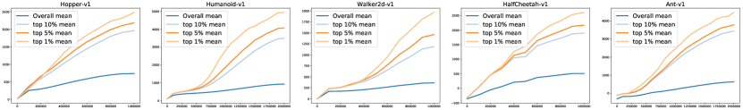
Figure 3: Training curves.

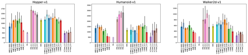
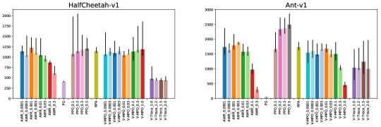
Figure 5: Comparison of 95th percentile of the performance of different policy losses conditioned on their hyperparameters.

          

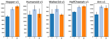
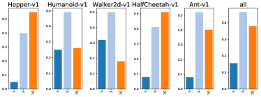
Figure 6: Analysis of choice num_epochs (CB.1): 95th percentile of performance scores conditioned on choice (left) and distribution of choices in top 5% of configurations (right).

          

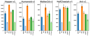
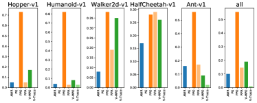
Figure 7: Analysis of choice Policy loss (CB.3): 95th percentile of performance scores conditioned on choice (left) and distribution of choices in top 5% of configurations (right).

          

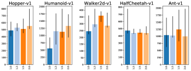
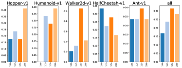
Figure 8: Analysis of choice V-Trace loss $\rho$ (C• ‣ B.3): 95th percentile of performance scores conditioned on sub-choice (left) and distribution of sub-choices in top 5% of configurations (right).

          

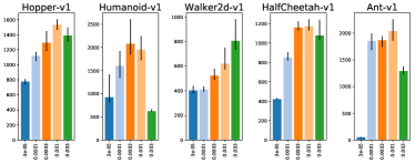
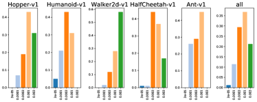
Figure 9: Analysis of choice Adam learning rate (CB.5): 95th percentile of performance scores conditioned on choice (left) and distribution of choices in top 5% of configurations (right).

          

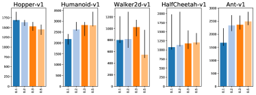
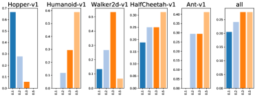
Figure 10: Analysis of choice PPO $\epsilon$ (C• ‣ B.3): 95th percentile of performance scores conditioned on sub-choice (left) and distribution of sub-choices in top 5% of configurations (right).

          

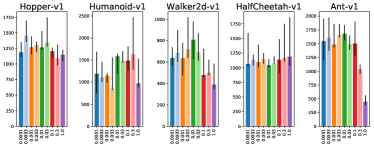
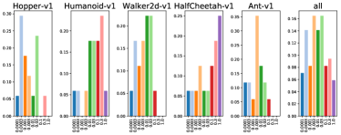
Figure 11: Analysis of choice V-MPO $\epsilon_{n}$ (C• ‣ B.3): 95th percentile of performance scores conditioned on sub-choice (left) and distribution of sub-choices in top 5% of configurations (right).

          

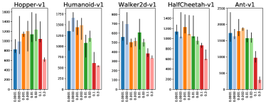
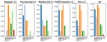
Figure 12: Analysis of choice AWR $\beta$ (C• ‣ B.3): 95th percentile of performance scores conditioned on sub-choice (left) and distribution of sub-choices in top 5% of configurations (right).

          

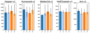
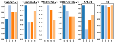
Figure 13: Analysis of choice AWR $\omega_{\texttt{max}}$ (C• ‣ B.3): 95th percentile of performance scores conditioned on sub-choice (left) and distribution of sub-choices in top 5% of configurations (right).

Appendix E Experiment Networks architecture

E.1 Design

For each of the 5 environments, we sampled 4000 choice configurations where we sampled the following choices independently and uniformly from the following ranges:

• Action transformation $T_{u}$ (C• ‣ B.8): {clip, tanh}

• Last value layer scaling (CB.7): {0.001, 0.01, 0.1, 1.0}

• Global standard deviation? (C• ‣ B.8): {False, True}

• Last policy layer scaling (CB.7): {0.001, 0.01, 0.1, 1.0}

• Standard deviation transformation $T_{\rho}$ (C• ‣ B.8): {exp, softplus}

• Initial standard deviation $i_{\rho}$ (C• ‣ B.8): {0.1, 0.5, 1.0, 2.0}

• Initializer (CB.7): {Glorot normal, Glorot uniform, He normal, He uniform, LeCun normal, LeCun uniform, Orthogonal, Orthogonal(gain=1.41)}

• Shared MLPs? (CB.7): {separate, shared}

  • For the case “Shared MLPs? (CB.7) = separate”, we further sampled the sub-choices:

    • Policy MLP width (CB.7): {16, 32, 64, 128, 256, 512}

    • Policy MLP depth (CB.7): {1, 2, 4, 8}

    • Value MLP width (CB.7): {16, 32, 64, 128, 256, 512}

    • Value MLP depth (CB.7): {1, 2, 4, 8}

  • For the case “Shared MLPs? (CB.7) = shared”, we further sampled the sub-choices:

    • Shared MLP width (CB.7): {16, 32, 64, 128, 256, 512}

    • Shared MLP depth (CB.7): {1, 2, 4, 8}

    • Baseline cost (shared) (CB.7): {0.001, 0.1, 1.0, 10.0, 100.0}

• Minimum standard deviation $\epsilon_{\rho}$ (C• ‣ B.8): {0.0, 0.01, 0.1}

• Adam learning rate (CB.5): {3e-05, 0.0001, 0.0003, 0.001}

• Activation (CB.7): {ELU, Leaky ReLU, ReLU, Sigmoid, Swish, Tanh}

All the other choices were set to the default values as described in Appendix C.

For each of the sampled choice configurations, we train 3 agents with different random seeds and compute the performance metric as described in Section 2.

After running the experiment described above we noticed (Fig. 15) that separate policy and value function networks (CB.7) perform better and we have rerun the experiment with only this variant present.

          

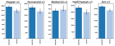
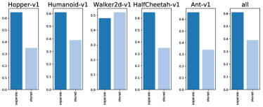
Figure 15: Analysis of choice Shared MLPs? (CB.7): 95th percentile of performance scores conditioned on choice (left) and distribution of choices in top 5% of configurations (right).

E.2 Results

We report aggregate statistics of the experiment in Table 4 as well as training curves in Figure 16. For each of the investigated choices in this experiment, we further provide a per-choice analysis in Figures 17-30.

Table 4: Performance quantiles across choice configurations.

	Ant-v1	HalfCheetah-v1	Hopper-v1	Humanoid-v1	Walker2d-v1
90th percentile	2098	1513	1133	1817	528
95th percentile	2494	2120	1349	2382	637
99th percentile	3138	3031	1582	3202	934
Max	4112	4358	1875	3987	1265

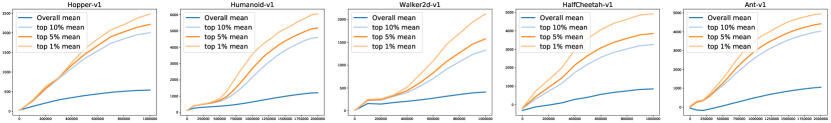
Figure 16: Training curves.

          

Figure 17: Analysis of choice Action transformation $T_{u}$ (C• ‣ B.8): 95th percentile of performance scores conditioned on choice (left) and distribution of choices in top 5% of configurations (right).

          

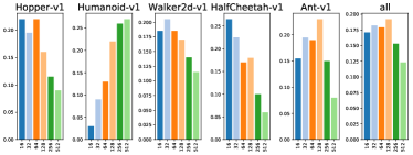
Figure 18: Analysis of choice Policy MLP width (CB.7): 95th percentile of performance scores conditioned on choice (left) and distribution of choices in top 5% of configurations (right).

          

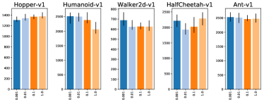
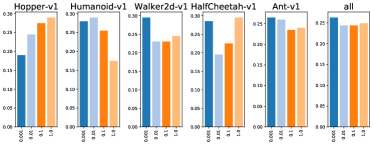
Figure 19: Analysis of choice Last value layer scaling (CB.7): 95th percentile of performance scores conditioned on choice (left) and distribution of choices in top 5% of configurations (right).

          

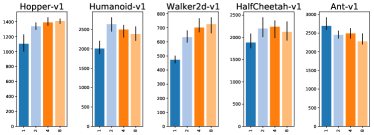
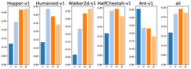
Figure 20: Analysis of choice Value MLP depth (CB.7): 95th percentile of performance scores conditioned on choice (left) and distribution of choices in top 5% of configurations (right).

          

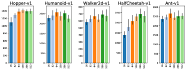
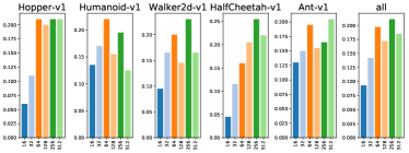
Figure 21: Analysis of choice Value MLP width (CB.7): 95th percentile of performance scores conditioned on choice (left) and distribution of choices in top 5% of configurations (right).

          

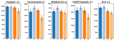
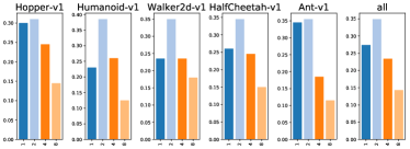
Figure 22: Analysis of choice Policy MLP depth (CB.7): 95th percentile of performance scores conditioned on choice (left) and distribution of choices in top 5% of configurations (right).

          

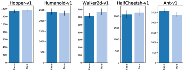
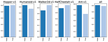
Figure 23: Analysis of choice Global standard deviation? (C• ‣ B.8): 95th percentile of performance scores conditioned on choice (left) and distribution of choices in top 5% of configurations (right).

          

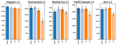
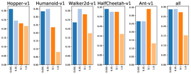
Figure 24: Analysis of choice Last policy layer scaling (CB.7): 95th percentile of performance scores conditioned on choice (left) and distribution of choices in top 5% of configurations (right).

          

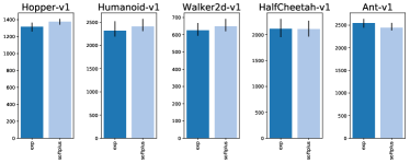
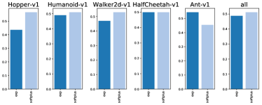
Figure 25: Analysis of choice Standard deviation transformation $T_{\rho}$ (C• ‣ B.8): 95th percentile of performance scores conditioned on choice (left) and distribution of choices in top 5% of configurations (right).

          

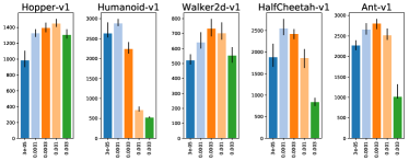
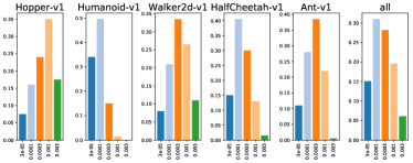
Figure 26: Analysis of choice Adam learning rate (CB.5): 95th percentile of performance scores conditioned on choice (left) and distribution of choices in top 5% of configurations (right).

          

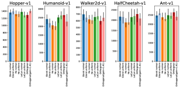
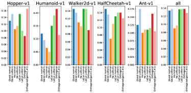
Figure 27: Analysis of choice Initializer (CB.7): 95th percentile of performance scores conditioned on choice (left) and distribution of choices in top 5% of configurations (right).

          

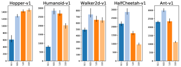
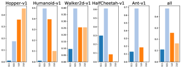
Figure 28: Analysis of choice Initial standard deviation $i_{\rho}$ (C• ‣ B.8): 95th percentile of performance scores conditioned on choice (left) and distribution of choices in top 5% of configurations (right).

          

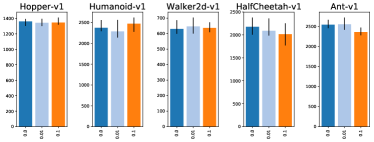
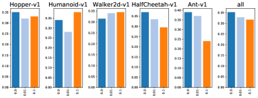
Figure 29: Analysis of choice Minimum standard deviation $\epsilon_{\rho}$ (C• ‣ B.8): 95th percentile of performance scores conditioned on choice (left) and distribution of choices in top 5% of configurations (right).

          

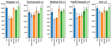
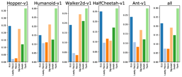
Figure 30: Analysis of choice Activation (CB.7): 95th percentile of performance scores conditioned on choice (left) and distribution of choices in top 5% of configurations (right).

Appendix F Experiment Normalization and clipping

F.1 Design

For each of the 5 environments, we sampled 2000 choice configurations where we sampled the following choices independently and uniformly from the following ranges:

• PPO $\epsilon$ (C• ‣ B.3): {0.1, 0.2, 0.3, 0.5}

• Input normalization (C• ‣ B.9): {Average, None}

  • For the case “Input normalization (C• ‣ B.9) = Average”, we further sampled the sub-choices:

    • Input clipping (C• ‣ B.9): {1.0, 2.0, 5.0, 10.0, None}

• Gradient clipping (C• ‣ B.9): {0.5, 1.0, 2.0, 5.0, None}

• Per minibatch advantage normalization (C• ‣ B.9): {False, True}

• Adam learning rate (CB.5): {3e-05, 0.0001, 0.0003, 0.001}

• Value function normalization (C• ‣ B.9): {Average, None}

All the other choices were set to the default values as described in Appendix C.

For each of the sampled choice configurations, we train 3 agents with different random seeds and compute the performance metric as described in Section 2.

F.2 Results

We report aggregate statistics of the experiment in Table 5 as well as training curves in Figure 31. For each of the investigated choices in this experiment, we further provide a per-choice analysis in Figures 32-38.

Table 5: Performance quantiles across choice configurations.

	Ant-v1	HalfCheetah-v1	Hopper-v1	Humanoid-v1	Walker2d-v1
90th percentile	2058	1265	1533	1649	1143
95th percentile	2287	1716	1662	2165	1564
99th percentile	2662	2465	1809	3100	2031
Max	3333	3515	2074	3482	2371

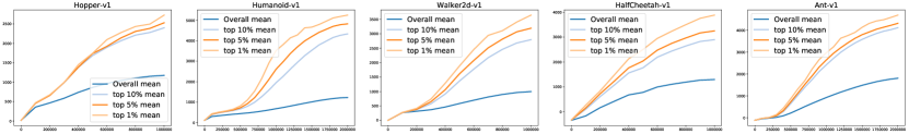
Figure 31: Training curves.

          

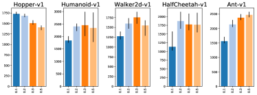
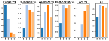
Figure 32: Analysis of choice PPO $\epsilon$ (C• ‣ B.3): 95th percentile of performance scores conditioned on choice (left) and distribution of choices in top 5% of configurations (right).

          

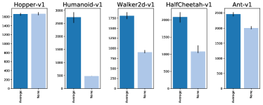
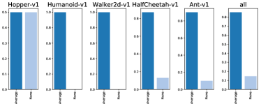
Figure 33: Analysis of choice Input normalization (C• ‣ B.9): 95th percentile of performance scores conditioned on choice (left) and distribution of choices in top 5% of configurations (right).

          

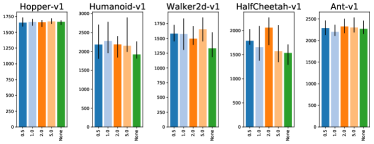
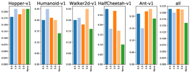
Figure 34: Analysis of choice Gradient clipping (C• ‣ B.9): 95th percentile of performance scores conditioned on choice (left) and distribution of choices in top 5% of configurations (right).

          

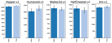
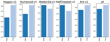
Figure 35: Analysis of choice Per minibatch advantage normalization (C• ‣ B.9): 95th percentile of performance scores conditioned on choice (left) and distribution of choices in top 5% of configurations (right).

          

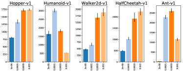
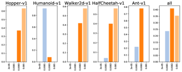
Figure 36: Analysis of choice Adam learning rate (CB.5): 95th percentile of performance scores conditioned on choice (left) and distribution of choices in top 5% of configurations (right).

          

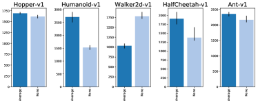
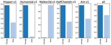
Figure 37: Analysis of choice Value function normalization (C• ‣ B.9): 95th percentile of performance scores conditioned on choice (left) and distribution of choices in top 5% of configurations (right).

          

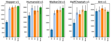
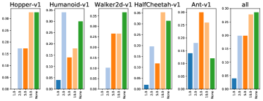
Figure 38: Analysis of choice Input clipping (C• ‣ B.9): 95th percentile of performance scores conditioned on sub-choice (left) and distribution of sub-choices in top 5% of configurations (right).

Appendix G Experiment Advantage Estimation

G.1 Design

For each of the 5 environments, we sampled 4000 choice configurations where we sampled the following choices independently and uniformly from the following ranges:

• num_envs (CB.1): {64, 128, 256}

• Value function loss (CB.2): {Huber, MSE}

  • For the case “Value function loss (CB.2) = Huber”, we further sampled the sub-choices:

    • Huber delta (CB.2): {0.001, 0.01, 0.1, 1.0}

• PPO-style value clipping $\epsilon$ (CB.2): {0.001, 0.01, 0.1, 1.0, None}

• advantage_estimator (CB.2): {GAE, N-step, V-Trace}

  • For the case “advantage_estimator (CB.2) = GAE”, we further sampled the sub-choices:

    • GAE $\lambda$ (C• ‣ B.2): {0.8, 0.9, 0.95, 0.99}

  • For the case “advantage_estimator (CB.2) = N-step”, we further sampled the sub-choices:

    • N-step $N$ (C• ‣ B.2): {1, 3, 10, 1000000}

  • For the case “advantage_estimator (CB.2) = V-Trace”, we further sampled the sub-choices:

    • V-Trace advantage $\lambda$ (C• ‣ B.2): {0.8, 0.9, 0.95, 0.99, 1.0}

    • V-Trace advantage $c,\,\rho$ (C• ‣ B.2): {1.0, 1.2, 1.5, 2.0}

• Adam learning rate (CB.5): {3e-05, 0.0001, 0.0003, 0.001, 0.003}

All the other choices were set to the default values as described in Appendix C.

For each of the sampled choice configurations, we train 3 agents with different random seeds and compute the performance metric as described in Section 2.

G.2 Results

We report aggregate statistics of the experiment in Table 6 as well as training curves in Figure 39. For each of the investigated choices in this experiment, we further provide a per-choice analysis in Figures 40-50.

Table 6: Performance quantiles across choice configurations.

	Ant-v1	HalfCheetah-v1	Hopper-v1	Humanoid-v1	Walker2d-v1
90th percentile	1705	1128	1626	1922	947
95th percentile	2114	1535	1777	2374	1185
99th percentile	2781	2631	2001	3013	1697
Max	3775	3613	2215	3564	2309

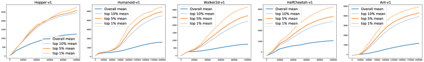
Figure 39: Training curves.

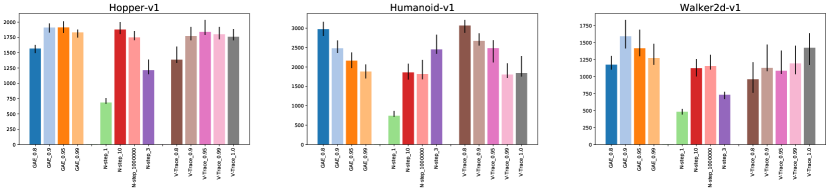
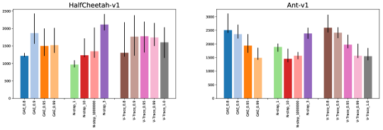
Figure 40: Comparison of 95th percentile of the performance of different advantage estimators conditioned on their hyperparameters.

          

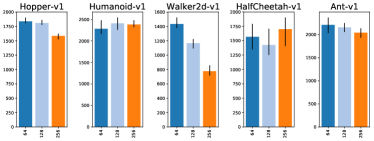
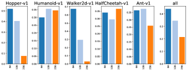
Figure 41: Analysis of choice num_envs (CB.1): 95th percentile of performance scores conditioned on choice (left) and distribution of choices in top 5% of configurations (right).

          

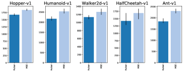
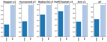
Figure 42: Analysis of choice Value function loss (CB.2): 95th percentile of performance scores conditioned on choice (left) and distribution of choices in top 5% of configurations (right).

          

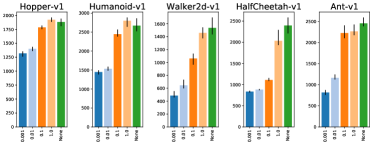
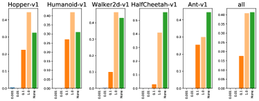
Figure 43: Analysis of choice PPO-style value clipping $\epsilon$ (CB.2): 95th percentile of performance scores conditioned on choice (left) and distribution of choices in top 5% of configurations (right).

          

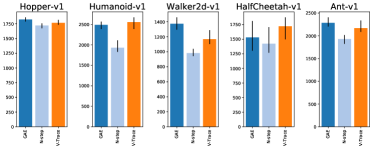
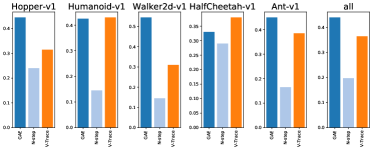
Figure 44: Analysis of choice advantage_estimator (CB.2): 95th percentile of performance scores conditioned on choice (left) and distribution of choices in top 5% of configurations (right).

          

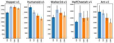
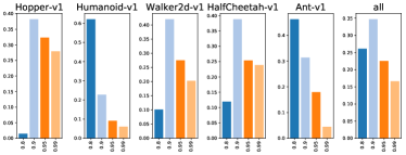
Figure 45: Analysis of choice GAE $\lambda$ (C• ‣ B.2): 95th percentile of performance scores conditioned on sub-choice (left) and distribution of sub-choices in top 5% of configurations (right).

          

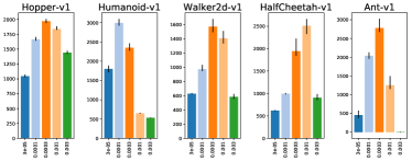
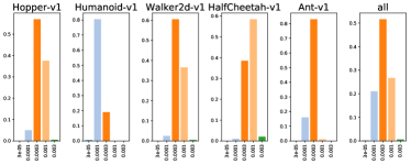
Figure 46: Analysis of choice Adam learning rate (CB.5): 95th percentile of performance scores conditioned on choice (left) and distribution of choices in top 5% of configurations (right).

          

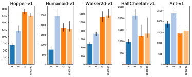
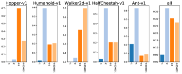
Figure 47: Analysis of choice N-step $N$ (C• ‣ B.2): 95th percentile of performance scores conditioned on sub-choice (left) and distribution of sub-choices in top 5% of configurations (right).

          

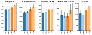
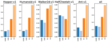
Figure 48: Analysis of choice Huber delta (CB.2): 95th percentile of performance scores conditioned on sub-choice (left) and distribution of sub-choices in top 5% of configurations (right).

          

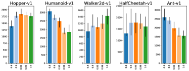
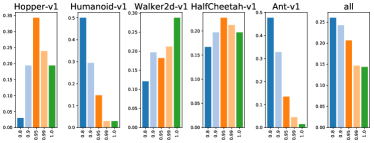
Figure 49: Analysis of choice V-Trace advantage $\lambda$ (C• ‣ B.2): 95th percentile of performance scores conditioned on sub-choice (left) and distribution of sub-choices in top 5% of configurations (right).

          

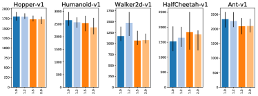
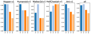
Figure 50: Analysis of choice V-Trace advantage $c,\,\rho$ (C• ‣ B.2): 95th percentile of performance scores conditioned on sub-choice (left) and distribution of sub-choices in top 5% of configurations (right).

Appendix H Experiment Training setup

H.1 Design

For each of the 5 environments, we sampled 2000 choice configurations where we sampled the following choices independently and uniformly from the following ranges:

• iteration_size (CB.1): {512, 1024, 2048, 4096}

• batch_mode (CB.1): {Fixed trajectories, Shuffle trajectories, Shuffle transitions, Shuffle transitions (recompute advantages)}

• num_epochs (CB.1): {1, 3, 10}

• num_envs (CB.1): {64, 128, 256}

• Adam learning rate (CB.5): {3e-05, 0.0001, 0.0003, 0.001, 0.003}

• batch_size (CB.1): {64, 128, 256}

All the other choices were set to the default values as described in Appendix C.

For each of the sampled choice configurations, we train 3 agents with different random seeds and compute the performance metric as described in Section 2.

H.2 Results

We report aggregate statistics of the experiment in Table 7 as well as training curves in Figure 51. For each of the investigated choices in this experiment, we further provide a per-choice analysis in Figures 52-58.

Table 7: Performance quantiles across choice configurations.

	Ant-v1	HalfCheetah-v1	Hopper-v1	Humanoid-v1	Walker2d-v1
90th percentile	2203	1316	1695	2310	1190
95th percentile	2484	1673	1853	2655	1431
99th percentile	2907	2665	2060	3014	1844
Max	3563	3693	2434	3502	2426

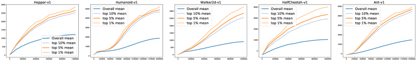
Figure 51: Training curves.

          

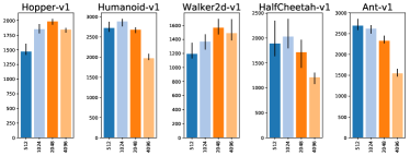
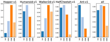
Figure 52: Analysis of choice iteration_size (CB.1): 95th percentile of performance scores conditioned on choice (left) and distribution of choices in top 5% of configurations (right).

          

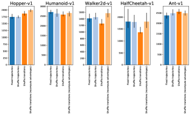
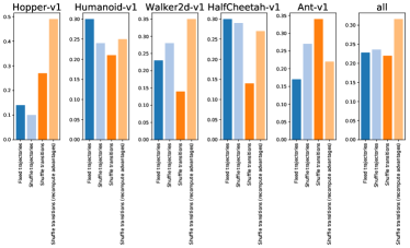
Figure 53: Analysis of choice batch_mode (CB.1): 95th percentile of performance scores conditioned on choice (left) and distribution of choices in top 5% of configurations (right).

          

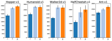
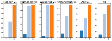
Figure 54: Analysis of choice num_epochs (CB.1): 95th percentile of performance scores conditioned on choice (left) and distribution of choices in top 5% of configurations (right).

          

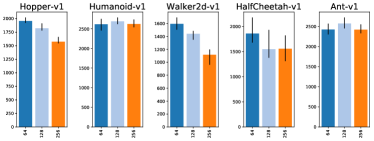
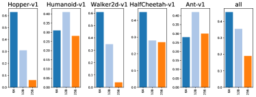
Figure 55: Analysis of choice num_envs (CB.1): 95th percentile of performance scores conditioned on choice (left) and distribution of choices in top 5% of configurations (right).

          

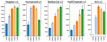
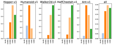
Figure 56: Analysis of choice Adam learning rate (CB.5): 95th percentile of performance scores conditioned on choice (left) and distribution of choices in top 5% of configurations (right).

          

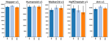
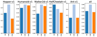
Figure 57: Analysis of choice batch_size (CB.1): 95th percentile of performance scores conditioned on choice (left) and distribution of choices in top 5% of configurations (right).

          

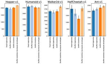
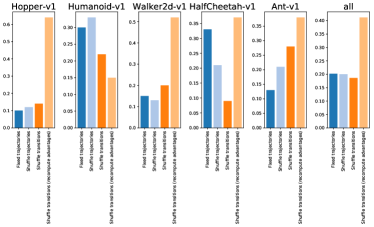
Figure 58: Analysis of choice batch_mode (CB.1): 95th percentile of performance scores conditioned on choice (left) and distribution of choices in top 5% of configurations(right). In order to obtain narrower confidence intervals in this experiment we only sweep batch_mode (CB.1), num_envs (CB.1), Adam learning rate (CB.5).

Appendix I Experiment Time

I.1 Design

For each of the 5 environments, we sampled 2000 choice configurations where we sampled the following choices independently and uniformly from the following ranges:

• Discount factor $\gamma$ (CB.4): {0.95, 0.97, 0.99, 0.999}

• Frame skip (CB.4): {1, 2, 5}

• Handle abandoned? (CB.4): {False, True}

• Adam learning rate (CB.5): {3e-05, 0.0001, 0.0003, 0.001}

All the other choices were set to the default values as described in Appendix C.

For each of the sampled choice configurations, we train 3 agents with different random seeds and compute the performance metric as described in Section 2.

I.2 Results

We report aggregate statistics of the experiment in Table 8 as well as training curves in Figure 59. For each of the investigated choices in this experiment, we further provide a per-choice analysis in Figures 60-63.

Table 8: Performance quantiles across choice configurations.

	Ant-v1	HalfCheetah-v1	Hopper-v1	Humanoid-v1	Walker2d-v1
90th percentile	1462	1063	1243	1431	761
95th percentile	1654	1235	1675	2158	810
99th percentile	2220	1423	2204	2769	974
Max	2833	1918	2434	3106	1431

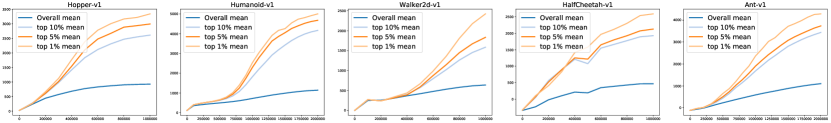
Figure 59: Training curves.

          

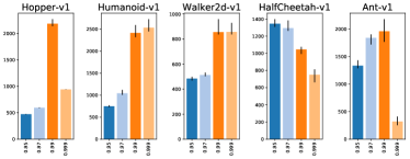
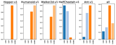
Figure 60: Analysis of choice Discount factor $\gamma$ (CB.4): 95th percentile of performance scores conditioned on choice (left) and distribution of choices in top 5% of configurations (right).

          

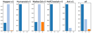
Figure 61: Analysis of choice Frame skip (CB.4): 95th percentile of performance scores conditioned on choice (left) and distribution of choices in top 5% of configurations (right).

          

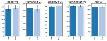
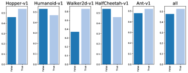
Figure 62: Analysis of choice Handle abandoned? (CB.4): 95th percentile of performance scores conditioned on choice (left) and distribution of choices in top 5% of configurations (right).

          

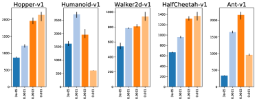
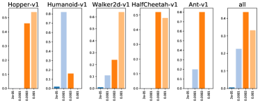
Figure 63: Analysis of choice Adam learning rate (CB.5): 95th percentile of performance scores conditioned on choice (left) and distribution of choices in top 5% of configurations (right).

Appendix J Experiment Optimizers

J.1 Design

For each of the 5 environments, we sampled 2000 choice configurations where we sampled the following choices independently and uniformly from the following ranges:

• Learning rate decay (CB.5): {0.0, 1.0}

• Optimizer (CB.5): {Adam, RMSProp}

  • For the case “Optimizer (CB.5) = Adam”, we further sampled the sub-choices:

    • Adam momentum (CB.5): {0.0, 0.9}

    • Adam $\epsilon$ (CB.5): {1e-09, 1e-08, 1e-07, 1e-06, 1e-05, 0.0001}

    • Adam learning rate (CB.5): {3e-05, 0.0001, 0.0003, 0.001}

  • For the case “Optimizer (CB.5) = RMSProp”, we further sampled the sub-choices:

    • RMSProp centered? (CB.5): {False, True}

    • RMSProp momentum (CB.5): {0.0, 0.9}

    • RMSProp $\epsilon$ (CB.5): {1e-09, 1e-08, 1e-07, 1e-06, 1e-05, 0.0001}

    • RMSProp learning rate (CB.5): {3e-05, 0.0001, 0.0003, 0.001}

All the other choices were set to the default values as described in Appendix C.

For each of the sampled choice configurations, we train 3 agents with different random seeds and compute the performance metric as described in Section 2.

J.2 Results

We report aggregate statistics of the experiment in Table 9 as well as training curves in Figure 64. For each of the investigated choices in this experiment, we further provide a per-choice analysis in Figures 65-73.

Table 9: Performance quantiles across choice configurations.

	Ant-v1	HalfCheetah-v1	Hopper-v1	Humanoid-v1	Walker2d-v1
90th percentile	2180	1085	1675	2549	712
95th percentile	2388	1124	1728	2726	797
99th percentile	2699	1520	1826	2976	1079
Max	2953	2532	1959	3332	1453

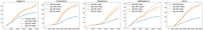
Figure 64: Training curves.

          

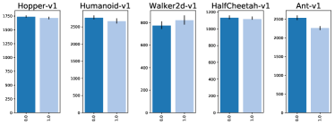
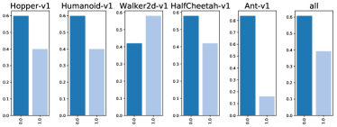
Figure 65: Analysis of choice Learning rate decay (CB.5): 95th percentile of performance scores conditioned on choice (left) and distribution of choices in top 5% of configurations (right).

          

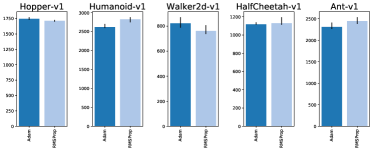
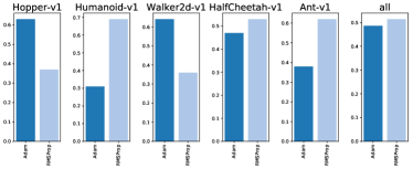
Figure 66: Analysis of choice Optimizer (CB.5): 95th percentile of performance scores conditioned on choice (left) and distribution of choices in top 5% of configurations (right).

          

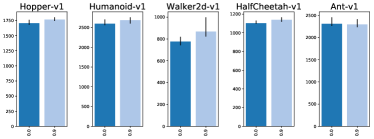
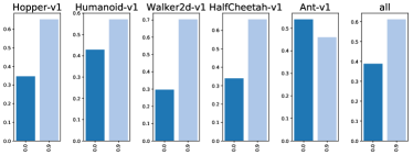
Figure 67: Analysis of choice Adam momentum (CB.5): 95th percentile of performance scores conditioned on sub-choice (left) and distribution of sub-choices in top 5% of configurations (right).

          

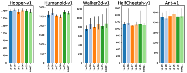
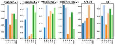
Figure 68: Analysis of choice Adam $\epsilon$ (CB.5): 95th percentile of performance scores conditioned on sub-choice (left) and distribution of sub-choices in top 5% of configurations (right).

          

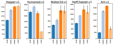
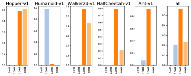
Figure 69: Analysis of choice Adam learning rate (CB.5): 95th percentile of performance scores conditioned on sub-choice (left) and distribution of sub-choices in top 5% of configurations (right).

          

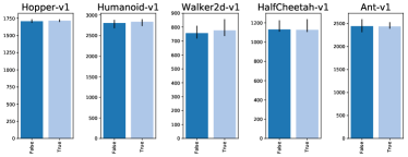
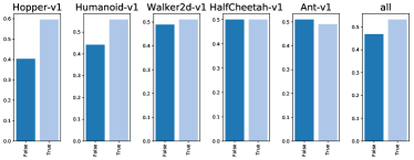
Figure 70: Analysis of choice RMSProp centered? (CB.5): 95th percentile of performance scores conditioned on sub-choice (left) and distribution of sub-choices in top 5% of configurations (right).

          

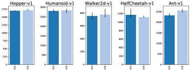
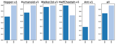
Figure 71: Analysis of choice RMSProp momentum (CB.5): 95th percentile of performance scores conditioned on sub-choice (left) and distribution of sub-choices in top 5% of configurations (right).

          

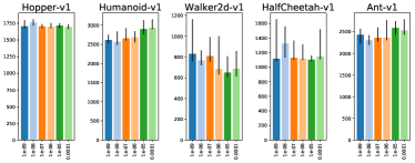
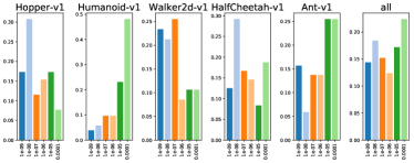
Figure 72: Analysis of choice RMSProp $\epsilon$ (CB.5): 95th percentile of performance scores conditioned on sub-choice (left) and distribution of sub-choices in top 5% of configurations (right).

          

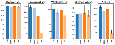
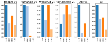
Figure 73: Analysis of choice RMSProp learning rate (CB.5): 95th percentile of performance scores conditioned on sub-choice (left) and distribution of sub-choices in top 5% of configurations (right).

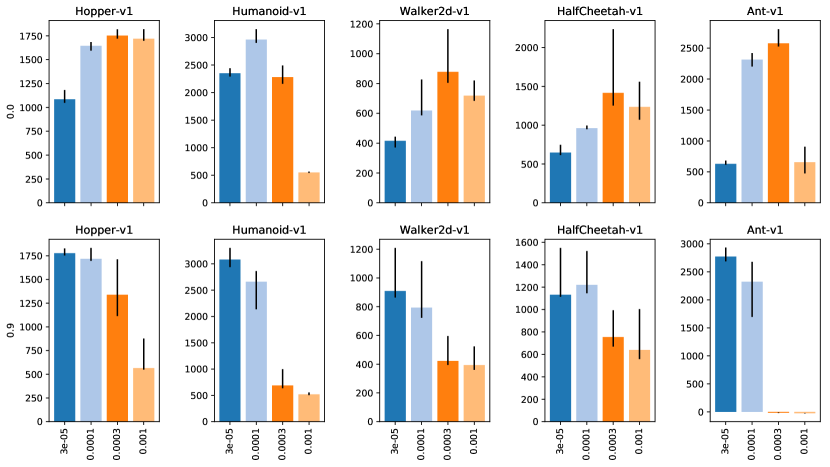
Figure 74: 95th percentile of performance scores conditioned on RMSProp momentum (CB.5)(rows) and RMSProp learning rate (CB.5)(bars).

Appendix K Experiment Regularizers

K.1 Design

For each of the 5 environments, we sampled 4000 choice configurations where we sampled the following choices independently and uniformly from the following ranges:

• Regularization type (CB.6): {Constraint, No regularization, Penalty}

  • For the case “Regularization type (CB.6) = Constraint”, we further sampled the sub-choices:

    • Regularizer (in case of constraint) (CB.6): {$\texttt{KL}(\mu||\pi)$, $\texttt{KL}(\pi||\mu)$, $\texttt{KL}(\texttt{ref}||\pi)$, decoupled $\texttt{KL}(\mu||\pi)$, entropy}

      • For the case “Regularizer (in case of constraint) (CB.6) = $\texttt{KL}(\mu||\pi)$”, we further sampled the sub-choices:

        • Threshold for $\texttt{KL}(\mu||\pi)$ (C1): {0.005, 0.01, 0.02, 0.04, 0.08}

      • For the case “Regularizer (in case of constraint) (CB.6) = $\texttt{KL}(\pi||\mu)$”, we further sampled the sub-choices:

        • Threshold for $\texttt{KL}(\pi||\mu)$ (C1): {0.005, 0.01, 0.02, 0.04, 0.08}

      • For the case “Regularizer (in case of constraint) (CB.6) = $\texttt{KL}(\texttt{ref}||\pi)$”, we further sampled the sub-choices:

        • Threshold for $\texttt{KL}(\texttt{ref}||\pi)$ (C1): {10.0, 20.0, 40.0, 80.0, 160.0}

      • For the case “Regularizer (in case of constraint) (CB.6) = decoupled $\texttt{KL}(\mu||\pi)$”, we further sampled the sub-choices:

        • Threshold for mean in decoupled $\texttt{KL}(\mu||\pi)$ (C1): {0.005, 0.01, 0.02, 0.04, 0.08}

        • Threshold for std in decoupled $\texttt{KL}(\mu||\pi)$ (C1): {5e-05, 0.000125, 0.00025, 0.0005, 0.001, 0.002, 0.004}

      • For the case “Regularizer (in case of constraint) (CB.6) = entropy”, we further sampled the sub-choices:

        • Threshold for entropy $H(\pi)$ (C1): {0.0, -5.0, -10.0, -15.0}

  • For the case “Regularization type (CB.6) = Penalty”, we further sampled the sub-choices:

    • Regularizer (in case of penalty) (CB.6): {$\texttt{KL}(\mu||\pi)$, $\texttt{KL}(\pi||\mu)$, $\texttt{KL}(\texttt{ref}||\pi)$, decoupled $\texttt{KL}(\mu||\pi)$, entropy}

      • For the case “Regularizer (in case of penalty) (CB.6) = $\texttt{KL}(\mu||\pi)$”, we further sampled the sub-choices:

        • Regularizer coefficient for $\texttt{KL}(\mu||\pi)$ (C1): {0.003, 0.01, 0.03, 0.1, 0.3, 1.0}

      • For the case “Regularizer (in case of penalty) (CB.6) = $\texttt{KL}(\pi||\mu)$”, we further sampled the sub-choices:

        • Regularizer coefficient for $\texttt{KL}(\pi||\mu)$ (C1): {0.003, 0.01, 0.03, 0.1, 0.3, 1.0}

      • For the case “Regularizer (in case of penalty) (CB.6) = $\texttt{KL}(\texttt{ref}||\pi)$”, we further sampled the sub-choices:

        • Regularizer coefficient for $\texttt{KL}(\texttt{ref}||\pi)$ (C1): {3e-06, 1e-05, 3e-05, 0.0001, 0.0003, 0.001}

      • For the case “Regularizer (in case of penalty) (CB.6) = decoupled $\texttt{KL}(\mu||\pi)$”, we further sampled the sub-choices:

        • Regularizer coefficient for mean in decoupled $\texttt{KL}(\mu||\pi)$ (C1): {0.003, 0.01, 0.03, 0.1, 0.3, 1.0}

        • Regularizer coefficient for std in decoupled $\texttt{KL}(\mu||\pi)$ (C1): {0.1, 0.3, 1.0, 3.0, 10.0, 30.0, 100.0, 300.0}

      • For the case “Regularizer (in case of penalty) (CB.6) = entropy”, we further sampled the sub-choices:

        • Regularizer coefficient for entropy (C1): {1e-05, 3e-05, 0.0001, 0.0003, 0.001, 0.003}

• Adam learning rate (CB.5): {3e-05, 0.0001, 0.0003, 0.001, 0.003}

All the other choices were set to the default values as described in Appendix C.

For each of the sampled choice configurations, we train 3 agents with different random seeds and compute the performance metric as described in Section 2.

K.2 Results

We report aggregate statistics of the experiment in Table 10 as well as training curves in Figure 75. For each of the investigated choices in this experiment, we further provide a per-choice analysis in Figures 76-92.

Table 10: Performance quantiles across choice configurations.

	Ant-v1	HalfCheetah-v1	Hopper-v1	Humanoid-v1	Walker2d-v1
90th percentile	2158	1477	1639	2624	705
95th percentile	2600	1870	1707	2832	814
99th percentile	2956	2413	1812	3071	1016
Max	3202	3156	1979	3348	1597

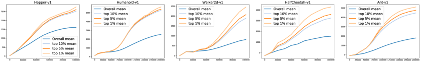
Figure 75: Training curves.

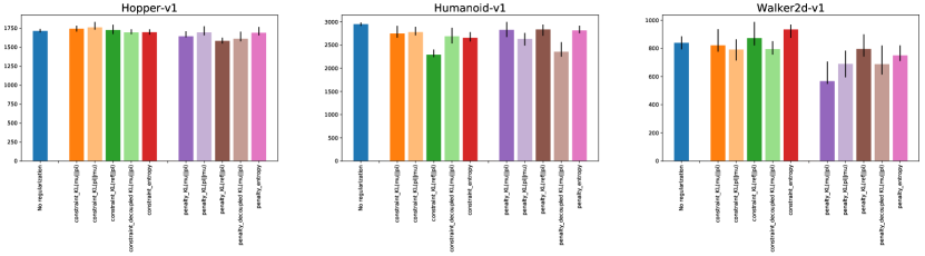
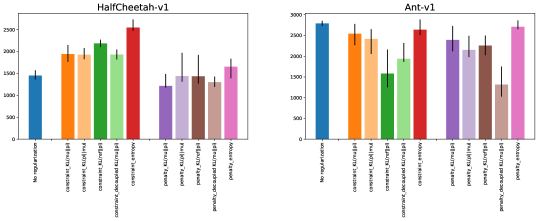
Figure 76: Comparison of 95th percentile of the performance of different regularization approaches conditioned on their type.

          

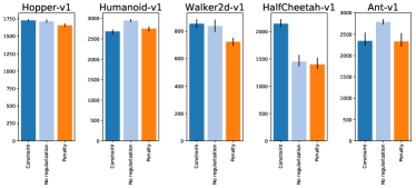
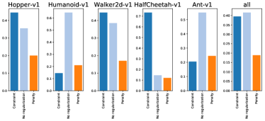
Figure 77: Analysis of choice Regularization type (CB.6): 95th percentile of performance scores conditioned on choice (left) and distribution of choices in top 5% of configurations (right).

          

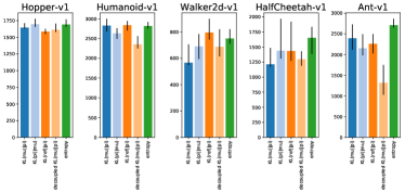
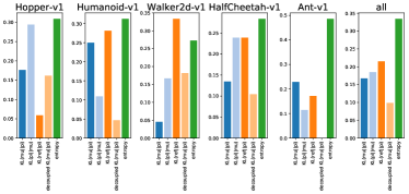
Figure 78: Analysis of choice Regularizer (in case of penalty) (CB.6): 95th percentile of performance scores conditioned on sub-choice (left) and distribution of sub-choices in top 5% of configurations (right).

          

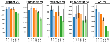
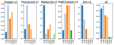
Figure 79: Analysis of choice Regularizer coefficient for $\texttt{KL}(\texttt{ref}||\pi)$ (C1): 95th percentile of performance scores conditioned on sub-choice (left) and distribution of sub-choices in top 5% of configurations (right).

          

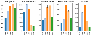
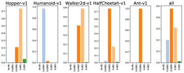
Figure 80: Analysis of choice Adam learning rate (CB.5): 95th percentile of performance scores conditioned on choice (left) and distribution of choices in top 5% of configurations (right).

          

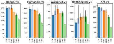
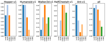
Figure 81: Analysis of choice Regularizer coefficient for entropy (C1): 95th percentile of performance scores conditioned on sub-choice (left) and distribution of sub-choices in top 5% of configurations (right).

          

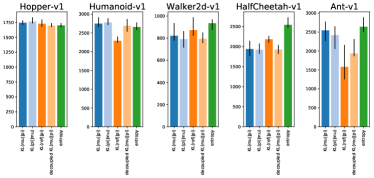
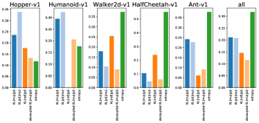
Figure 82: Analysis of choice Regularizer (in case of constraint) (CB.6): 95th percentile of performance scores conditioned on sub-choice (left) and distribution of sub-choices in top 5% of configurations (right).

          

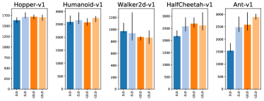
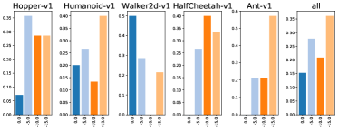
Figure 83: Analysis of choice Threshold for entropy $H(\pi)$ (C1): 95th percentile of performance scores conditioned on sub-choice (left) and distribution of sub-choices in top 5% of configurations (right).

          

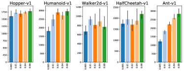
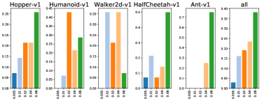
Figure 84: Analysis of choice Threshold for $\texttt{KL}(\mu||\pi)$ (C1): 95th percentile of performance scores conditioned on sub-choice (left) and distribution of sub-choices in top 5% of configurations (right).

          

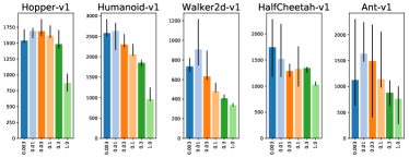
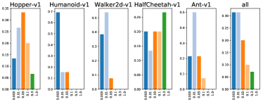
Figure 85: Analysis of choice Regularizer coefficient for mean in decoupled $\texttt{KL}(\mu||\pi)$ (C1): 95th percentile of performance scores conditioned on sub-choice (left) and distribution of sub-choices in top 5% of configurations (right).

          

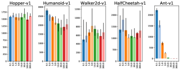
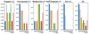
Figure 86: Analysis of choice Regularizer coefficient for std in decoupled $\texttt{KL}(\mu||\pi)$ (C1): 95th percentile of performance scores conditioned on sub-choice (left) and distribution of sub-choices in top 5% of configurations (right).

          

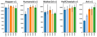
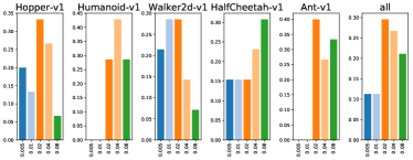
Figure 87: Analysis of choice Threshold for $\texttt{KL}(\pi||\mu)$ (C1): 95th percentile of performance scores conditioned on sub-choice (left) and distribution of sub-choices in top 5% of configurations (right).

          

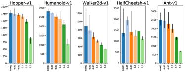
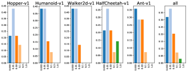
Figure 88: Analysis of choice Regularizer coefficient for $\texttt{KL}(\pi||\mu)$ (C1): 95th percentile of performance scores conditioned on sub-choice (left) and distribution of sub-choices in top 5% of configurations (right).

          

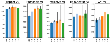
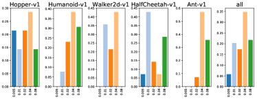
Figure 89: Analysis of choice Threshold for mean in decoupled $\texttt{KL}(\mu||\pi)$ (C1): 95th percentile of performance scores conditioned on sub-choice (left) and distribution of sub-choices in top 5% of configurations (right).

          

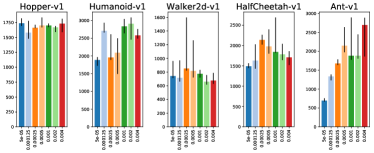
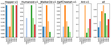
Figure 90: Analysis of choice Threshold for std in decoupled $\texttt{KL}(\mu||\pi)$ (C1): 95th percentile of performance scores conditioned on sub-choice (left) and distribution of sub-choices in top 5% of configurations (right).

          

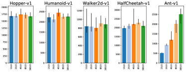
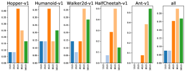
Figure 91: Analysis of choice Threshold for $\texttt{KL}(\texttt{ref}||\pi)$ (C1): 95th percentile of performance scores conditioned on sub-choice (left) and distribution of sub-choices in top 5% of configurations (right).

          

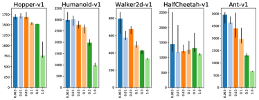
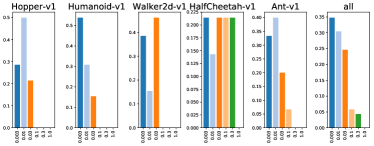
Figure 92: Analysis of choice Regularizer coefficient for $\texttt{KL}(\mu||\pi)$ (C1): 95th percentile of performance scores conditioned on sub-choice (left) and distribution of sub-choices in top 5% of configurations (right).

References

- [1] Peter J Huber “Robust estimation of a location parameter” In Breakthroughs in statistics Springer, 1992, pp. 492–518
- [2] Ronald J Williams “Simple statistical gradient-following algorithms for connectionist reinforcement learning” In Machine learning 8.3-4 Springer, 1992, pp. 229–256
- [3] Richard S Sutton and Andrew G Barto “Introduction to reinforcement learning” MIT press Cambridge, 1998
- [4] Brian D Ziebart “Modeling purposeful adaptive behavior with the principle of maximum causal entropy”, 2010
- [5] Emanuel Todorov, Tom Erez and Yuval Tassa “Mujoco: A physics engine for model-based control” In 2012 IEEE/RSJ International Conference on Intelligent Robots and Systems, 2012, pp. 5026–5033 IEEE
- [6] Volodymyr Mnih et al. “Playing atari with deep reinforcement learning” In arXiv preprint arXiv:1312.5602, 2013
- [7] Kaiming He, Xiangyu Zhang, Shaoqing Ren and Jian Sun “Delving deep into rectifiers: Surpassing human-level performance on imagenet classification” In Proceedings of the IEEE international conference on computer vision, 2015, pp. 1026–1034
- [8] Diederik P. Kingma and Jimmy Ba “Adam: A Method for Stochastic Optimization” In 3rd International Conference on Learning Representations, ICLR 2015, San Diego, CA, USA, May 7-9, 2015, Conference Track Proceedings, 2015 URL: http://arxiv.org/abs/1412.6980
- [9] John Schulman et al. “High-dimensional continuous control using generalized advantage estimation” In arXiv preprint arXiv:1506.02438, 2015
- [10] John Schulman et al. “Trust region policy optimization” In International conference on machine learning, 2015, pp. 1889–1897
- [11] Martin Abadi et al. “Tensorflow: A system for large-scale machine learning” In 12th USENIX Symposium on Operating Systems Design and Implementation (OSDI 16), 2016, pp. 265–283
- [12] Greg Brockman et al. “Openai gym” In arXiv preprint arXiv:1606.01540, 2016
- [13] Timothy P Lillicrap et al. “Continuous control with deep reinforcement learning” In International Conference on Learning Representations, 2016
- [14] Volodymyr Mnih et al. “Asynchronous methods for deep reinforcement learning” In International conference on machine learning, 2016, pp. 1928–1937
- [15] Riashat Islam, Peter Henderson, Maziar Gomrokchi and Doina Precup “Reproducibility of benchmarked deep reinforcement learning tasks for continuous control” In arXiv preprint arXiv:1708.04133, 2017
- [16] Fabio Pardo, Arash Tavakoli, Vitaly Levdik and Petar Kormushev “Time limits in reinforcement learning” In arXiv preprint arXiv:1712.00378, 2017
- [17] John Schulman et al. “Proximal policy optimization algorithms” In arXiv preprint arXiv:1707.06347, 2017
- [18] Abbas Abdolmaleki et al. “Maximum a posteriori policy optimisation” In arXiv preprint arXiv:1806.06920, 2018
- [19] Lasse Espeholt et al. “IMPALA: Scalable Distributed Deep-RL with Importance Weighted Actor-Learner Architectures” In International Conference on Machine Learning, 2018, pp. 1406–1415
- [20] Tuomas Haarnoja et al. “Soft actor-critic algorithms and applications” In arXiv preprint arXiv:1812.05905, 2018
- [21] Tuomas Haarnoja, Aurick Zhou, Pieter Abbeel and Sergey Levine “Soft Actor-Critic: Off-Policy Maximum Entropy Deep Reinforcement Learning with a Stochastic Actor” In International Conference on Machine Learning, 2018, pp. 1861–1870
- [22] Peter Henderson et al. “Deep reinforcement learning that matters” In Thirty-Second AAAI Conference on Artificial Intelligence, 2018
- [23] Francesco Locatello et al. “Challenging common assumptions in the unsupervised learning of disentangled representations” In arXiv preprint arXiv:1811.12359, 2018
- [24] Mario Lucic et al. “Are gans created equal? a large-scale study” In Advances in neural information processing systems, 2018, pp. 700–709
- [25] M Andrychowicz OpenAI et al. “Learning dexterous in-hand manipulation” In arXiv preprint arXiv:1808.00177 no, 2018
- [26] George Tucker et al. “The mirage of action-dependent baselines in reinforcement learning” In arXiv preprint arXiv:1802.10031, 2018
- [27] Logan Engstrom et al. “Implementation Matters in Deep RL: A Case Study on PPO and TRPO” In International Conference on Learning Representations, 2019
- [28] Lasse Espeholt et al. “SEED RL: Scalable and Efficient Deep-RL with Accelerated Central Inference” In arXiv preprint arXiv:1910.06591, 2019
- [29] Michael Janner, Justin Fu, Marvin Zhang and Sergey Levine “When to trust your model: Model-based policy optimization” In Advances in Neural Information Processing Systems, 2019, pp. 12498–12509
- [30] Alex Kendall et al. “Learning to drive in a day” In 2019 International Conference on Robotics and Automation (ICRA), 2019, pp. 8248–8254 IEEE
- [31] Eric Langlois et al. “Benchmarking model-based reinforcement learning” In arXiv preprint arXiv:1907.02057, 2019
- [32] Ilge OpenAI et al. “Solving Rubik’s Cube with a Robot Hand” In arXiv preprint arXiv:1910.07113, 2019
- [33] Xue Bin Peng, Aviral Kumar, Grace Zhang and Sergey Levine “Advantage-Weighted Regression: Simple and Scalable Off-Policy Reinforcement Learning” In arXiv preprint arXiv:1910.00177, 2019
- [34] H Francis Song et al. “V-MPO: On-Policy Maximum a Posteriori Policy Optimization for Discrete and Continuous Control” In arXiv preprint arXiv:1909.12238, 2019
- [35] Jared Kaplan et al. “Scaling laws for neural language models” In arXiv preprint arXiv:2001.08361, 2020
- [36] Ilija Radosavovic et al. “Designing Network Design Spaces” In arXiv preprint arXiv:2003.13678, 2020