Understanding Noise Injection in GANs

Abstract

Noise injection is an effective way of circumventing overfitting and enhancing generalization in machine learning, the rationale of which has been validated in deep learning as well. Recently, noise injection exhibits surprising effectiveness when generating high-fidelity images in Generative Adversarial Networks (GANs) (e.g. StyleGAN). Despite its successful applications in GANs, the mechanism of its validity is still unclear. In this paper, we propose a geometric framework to theoretically analyze the role of noise injection in GANs. First, we point out the existence of the adversarial dimension trap inherent in GANs, which leads to the difficulty of learning a proper generator. Second, we successfully model the noise injection framework with exponential maps based on Riemannian geometry. Guided by our theories, we propose a general geometric realization for noise injection. Under our novel framework, the simple noise injection used in StyleGAN reduces to the Euclidean case. The goal of our work is to make theoretical steps towards understanding the underlying mechanism of state-of-the-art GAN algorithms. Experiments on image generation and GAN inversion validate our theory in practice.

1 Introduction

Noise injection is usually applied as regularization to cope with overfitting or facilitate generalization in neural networks (Bishop, 1995; An, 1996). The effectiveness of this simple technique has also been proved in various tasks in deep learning, such as learning deep architectures (Hinton et al., 2012; Srivastava et al., 2014; Noh et al., 2017), defending adversarial attacks (He et al., 2019), facilitating stability of differentiable architecture search with reinforcement learning (Liu et al., 2019; Chu et al., 2020), and quantizing neural networks (Baskin et al., 2018). In recent years, noise injection has attracted more and more attention in the community of Generative Adversarial Networks (GANs) (Goodfellow et al., 2014a). Extensive research shows that it helps stabilize the training procedure (Arjovsky & Bottou, 2017; Jenni & Favaro, 2019) and generate images of high fidelity (Karras et al., 2019a, b; Brock et al., 2018).

$\longrightarrow$ Increasing noise injection depth	Standard Dev

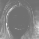
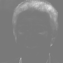
Figure 1: Noise injection significantly improves the detail quality of generated images. From left to right, we inject extra noise to the generator layer by layer. We can see that hair quality is clearly improved. Varying the injected noise and visualizing the standard deviation over 100 different seeds, we can find that the detailed information such as hair, parts of the background, and silhouettes are most involved, while the global information such as identity and pose is less affected.

Particularly, noise injection in StyleGAN (Karras et al., 2019a, b) has shown the amazing capability of helping generate sharp details in images (see Fig. 1 for illustration), shedding new light on obtaining high-quality photo-realistic results using GANs. Therefore, studying the underlying principle of noise injection in GANs is an important theoretical work of understanding GAN algorithms.

In this paper, we propose a theoretical framework to explain and improve the effectiveness of noise injection in GANs. Our contributions are listed as follows:

• we uncover an intrinsic defect of GAN models that the expressive power of generator is limited by the rank of its Jacobian matrix, and the rank of Jacobian matrix is monotonically (but not strictly) decreasing as the network gets deeper.

• We prove that noise injection is an effective weapon to enhance the expressive power of generators for GANs.

• Based on our theory, we propose a generalized form for noise injection in GANs, which can overcome the adversarial dimension trap. Experiments on the state-of-the-art GAN, StyleGAN2 (Karras et al., 2019b), validate the effectiveness of our geometric model.

To the best of our knowledge, this is the first work that theoretically draws the geometric picture of noise injection in GANs, and uncover the intrinsic defect of the expressive power of generators.

2 Related Work

The main drawbacks of GANs are unstable training and mode collapse. Arjovsky et al. (Arjovsky & Bottou, 2017) theoretically analyze that noise injection to the image space can help smooth the distribution so as to stabilize the training. The authors of Distribution-Filtering GAN (DFGAN) (Jenni & Favaro, 2019) then put this idea into practice and prove that this technique will not influence the global optimality of the real data distribution. However, as the authors pointed out in (Arjovsky & Bottou, 2017), this method depends on the amount of noise, and does not support the intrinsic geometry of synthesis and data distributions. Actually, our method of noise injection is essentially different from these ones as we conduct it in the feature spaces. Besides, they do not provide a theoretical vision of explaining the connection between injected noise and features.

BigGAN (Brock et al., 2018) splits input latent vectors into one chunk per layer and projects each chunk to the gains and biases of batch normalization in each layer. They claim that this design allows direct influence on features at different resolutions and levels of hierarchy. StyleGAN (Karras et al., 2019a) and StyleGAN2 (Karras et al., 2019b) adopt a slightly different view, where noise injection is introduced to enhance randomness for multi-scale stochastic variations. Different from the settings in BigGAN, they inject extra noise independent of latent inputs into different layers of the network without projection. Our theoretical analysis is mainly motivated by the success of noise injection used in StyleGAN (Karras et al., 2019a). Our proposed framework reveals that noise injection in StyleGAN is a kind of reparameterization in Euclidean spaces, and we extend it into generic manifolds (section 4.3).

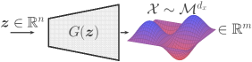
Figure 2: Illustration of dimensions in the generator of GAN. We assume that the data $\mathcal{X}$ lie in an underlying low-dimensional manifold $\mathcal{M}^{d_{x}}$ embedded in the high-dimensional Euclidean space $\mathbb{R}^{m}$, where $d_{x}$ is the intrinsic dimension of $\mathcal{M}$ and $m$ is the ambient dimension. Usually, we have $d_{x}\ll m$ and $n\ll m$.

3 Inherent Drawbacks of GANs

We will analyze the inherent drawbacks of traditional GANs in this section. Our arguments can be divided into three steps. We first prove that the rank of Jacobian matrix limits the intrinsic dimension of the learned manifold of the generator. Then we show that the rank of Jacobian matrix monotonically decreases as the network gets deeper. At last we prove that the expressive power of learned distribution is limited by its intrinsic dimension.

Prior to our arguments, we briefly introduce the geometric perspective of generative models as follows. Given a prior $z$, the generator $G$ of GAN generates a fake sample $\tilde{x}=G(z)$. Here, the fake sample is of the same ambient dimension with the real sample set $\mathcal{X}$ in the Euclidean space $\mathbb{R}^{m}$. The input prior $z$ is a $n$-dimensional vector, which is usually sampled from Gaussian distributions of $\mathbb{R}^{n}$. Following the convention of manifold learning (Tenenbaum et al., 2000; Roweis & Saul, 2000), we assume that the real data $\mathcal{X}$ lie in an underlying low-dimensional manifold $\mathcal{M}^{d_{x}}$ embedded in the high-dimensional $\mathbb{R}^{m}$, where $d_{x}$ is called the intrinsic dimension of $\mathcal{M}$ and $m$ is the ambient dimension using the geometric language. Usually, we have $d_{x}\ll m$ and $n\ll m$, e.g. $n=512$ and $m=1024\times 1024\times 3$ in StyleGAN. The generation process and related dimensions are illustrated in Figure 2. The intrinsic dimension $d_{x}$ is actually ambiguous in most cases, thus making the generation problem complicated. We refer to the dimension of the data manifold as the intrinsic dimension $d_{x}$ except noted otherwise. The purpose of GAN is then to approximate this data manifold $\mathcal{M}^{d_{x}}$ with generator-induced manifold $\mathcal{G}^{d_{g}}=G(\mathcal{Z})$.

3.1 Jacobian Limits the Intrinsic Dimension

We first prove that the intrinsic dimension $d_{g}$ of the generated distribution can be identified through the Jacobian matrix of the generator.

Definition 1 (Jacobian matrix).

Let $f:\mathcal{Z}\rightarrow\mathbb{R}^{m}$, where $\mathcal{Z}$ are open subset in $\mathbb{R}^{n}$. Let

$$\frac{df_{i}}{dz_{j}}(z)=\lim\limits_{h\rightarrow 0}\frac{f_{i}(z+he_{j})}{h},\vspace{-0.15cm}$$ (1)

where $e_{j}\in\mathbb{R}^{n}$ is a vector with the $j$-th component to be 1 and 0 otherwise, and $f_{i}$ is the $i$-th component of $f$. Then the Jacobian matrix of $f$ with respect to variable $z$ is the matrix

$$J_{z}f=\left(\frac{df_{i}}{dz_{j}}(z)\right)_{m\times n}.\vspace{-0.15cm}$$ (2)

Lemma 1.

Let $f:\mathbb{R}^{n}\rightarrow\mathbb{R}^{m}$ and $f(\mathcal{Z})=\mathcal{X}^{d_{f}}$ be a manifold embedded in $\mathbb{R}^{m}$ with $\mathcal{Z}$ an open subset of $\mathbb{R}^{n}$. Then for almost every point $x\in\mathcal{X}^{d_{f}}$, the gradient matrix of $f$ has constant rank $rank(J_{z}f)$ at the preimage of $x$ in $\mathcal{Z}$, and the intrinsic dimension of $\mathcal{X}^{d_{f}}$ is $d_{f}=rank(J_{z}f)$.

When $f$ is a linear transformation, i.e. $f(x)=Ax,A\in\mathbb{R}^{m\times n}$, Lemma 1 reduces to rank theorem of matrices (Strang et al., 1993), that the dimension of subspace induced by a matrix is equal to the rank of that matrix.

Lemma 1 gives a quantitative description to the property of generated manifold $\mathcal{G}^{d_{g}}$, that it has an intrinsic dimension equal to the rank of $J_{z}G\in\mathbb{R}^{n\times m}$. Recall that a matrix of $\mathbb{R}^{m\times n}$ has rank at most $\min\{n,m\}$. Thus we have $d_{g}\leq\min\{n,m\}$. In practice, the prior dimension $n$ is usually a bit small compared with the high variance of details in real-world data. Taking face images as an example, the hair, freckles, and wrinkles have an extremely high degree of freedom, the combination of which may exceed millions of types, while typical GANs only have latent dimensions around 512. In order to plausibly model the detail of images, we might need to bring more ‘freedom’ to the network.

3.2 Monotonic Decreasing of Jacobian Rank

Apart from the relatively small prior dimension, another trouble comes from the network depth. To capture highly non-linear features of data manifolds, current generators often use a very deep coupling of CNN modules. The following Lemma then suggests a sustained decline in the dimension of the generated manifold as the network gets deeper.

Lemma 2.

Let $f=f^{1}\circ f^{2}$, then we have $rank(Jf)\leq\min\{rank(Jf^{1}),rank(Jf^{2})\}$. Specifically, let $F^{k}=f^{1}\circ f^{2}\circ\dots\circ f^{k}$, we have $rank(JF^{s})\leq rank(JF^{t})$ if $s\geq t$, and $rank(JF^{s})\leq rank(Jf^{k})$ for all $k\leq s$.

Typical generators are composed of a large number of CNN and MLP blocks, which will keep reducing the dimension of the feature manifolds during the feedforward procedure. The intention of reducing the feature dimension in the deep generator network, combined with the relatively low prior dimension and Lemma 1, will then force the dimension of the generated manifold lower than that of the real data manifold. We will look into how this will influence the expressive power of GANs.

3.3 Adversarial Dimension Trap

Previous sections have demonstrated that, in practice, there is a very high chance that the generated manifold has an intrinsic dimension lower than the data manifold’s. During training, however, the discriminator which measures the distance of these two distributions will keep encouraging the generator to increase the dimension up to the same as the true data. This contradictory functionality, as we show in the theorem below, incurs severe punishment on the smoothness and invertibility of the generative model, which we refer to as the adversarial dimension trap.

Theorem 1.

For a deterministic GAN model and generator $G:\mathcal{Z}\rightarrow\mathcal{X}$, if $rank(J_{z}G)<d_{x}$, then at least one of the two cases must stand:

1. $\sup_{z\in\mathcal{Z}}\|J_{z}G\|=\infty$;

2. the generator network fails to capture the data distribution and is unable to perform inversion. Namely, for an arbitrary point $x\in\mathcal{X}$, the possibility of $G^{-1}(x)=\emptyset$ is 1, and we have the following estimation

   $$D_{JS}(\mathbb{P}_{g},\mathbb{P}_{r})\geq\frac{\log 2}{2},\vspace{-0.15cm}$$ (3)

   where $D_{JS}$ is the Jensen-Shannon divergence, $\mathbb{P}_{g}$ and $\mathbb{P}_{r}$ are generated and data distributions, respectively.

The above theorem stands for a wide range of GAN loss functions, including Wasserstein divergence, Jensen-Shannon divergence, and other KL-divergence based losses. Notice that this theorem implies a much worse situation than it states. For any open sphere $B$ in the data manifold $\mathcal{X}$, the generator restricted in the pre-image of $B$ also follows this theorem, which suggests bad properties of nearly every local neighborhood. This also suggests that the above consequences of Theorem 1 may both stand. As in some subsets, the generator may successfully capture the data distribution, while in some others, the generator may fail to do so.

The above theorem describes the relationship between $rank(J_{z}G)$ and the expressive power of GANs. It means that a generator with a very small Jacobian rank may not be able to model complicated manifolds. We will show how noise injection addresses this issue.

The readers may note that, our expressive power here is a bit different from those in classification tasks. For example, in a binary classification task, the intrinsic dimension of output space is the same as its ambient space. The expressive power in this case cares more about modeling the highly non-linear structure of it. While in this paper, as our target is a data manifold with unknown intrinsic dimension, the expressive power focuses on capturing all its intrinsic dimensions, which corresponds to certain semantic features of images.

(a) Skeleton of the manifold.	(b) Representative pair.

Figure 3: Illustration of the skeleton set and representative pair. The blue curve in (a) is the skeleton. In (b), the dashed sphere in $\mathcal{M}$ is the geodesic ball, while the solid sphere in $\mathcal{T}_{\mu}\mathcal{M}$ is its projection onto the tangent space. The normal vector $\vec{n}$ determines the final affine transformation into the Euclidean space.

4 Riemannian Geometry of Noise Injection

The generator $G$ in the traditional GAN is a composite of sequential non-linear feature mappings, which can be denoted as $G(z)=f^{k}\circ f^{k-1}\circ\dots\circ f^{1}(z)$, where $z\sim\mathcal{N}(0,1)$ is the standard Gaussian. Each feature mapping is typically a single layer convolutional neural network (CNN) combined with non-linear operations such as normalization, pooling, and activation. The whole network is then a deterministic mapping from the latent space $\mathcal{Z}$ to the image space $\mathcal{X}$. The common noise injection is actually a linear transformation

$$f^{k}\leftarrow f^{k}+a\epsilon,~{}\epsilon\sim\mathcal{N}(0,1),\vspace{-0.15cm}$$ (4)

where $a$ is a learnable scalar parameter and noise $\epsilon$ is randomly sampled from Gaussian $\mathcal{N}(0,1)$. This simple technique significantly improves the performance of GANs, especially the fidelity and realism of generated images as displayed in Figure 1.

In order to establish a solid geometric framework, we propose a general formulation by replacing $f^{k}(x)$ with

$$g^{k}(x)=\mu^{k}(x)+\sigma^{k}(x)\epsilon,~{}x\in g^{k-1}\circ\dots\circ g^{1}(\mathcal{Z}),$$ (5)

where $\mu^{k}(x)$ and $\sigma^{k}(x)$ are both learnable weight matrices. It is straightforward to see that noise injection in (5), which is a type of deep noise injection in feature maps of each layer, is essentially different from the reparameterization trick used in VAEs (Kingma & Welling, 2013) that is only applied to the final outputs. In what follows, we call (5) used in this paper Riemannian Noise Injection (RNI) as our theory is established with Riemannian geometry.

It is worth emphasizing that RNI in (5) can be viewed as fuzzy equivalence relation of the original features, and uses reparameterization to model the low-dimensional feature manifolds. We present this content in the supplementary material for interested readers.

4.1 Handling Adversarial Dimension Trap with Noise Injection

As Sard’s theorem tells us (Petersen et al., 2006), the key to solving the adversarial dimension trap is to avoid mapping low-dimensional feature spaces into feature manifolds with higher intrinsic dimensions. However, we are not able to control the intrinsic dimension of data manifold, and in each intermediate feature spaces of the network, we are threatened by the intention of dimension drop in Lemma 2. So the solution could be that, instead of learning mappings into the full feature spaces, we choose to map only onto the skeleton of the each feature spaces and use random noise to fill up the remaining space. For a compact manifold, it is easy to find that the intrinsic dimension of the skeleton set can be arbitrarily low by applying Heine–Borel theorem to the skeleton (Rudin et al., 1964). By this way, the model can escape from the adversarial dimension trap.

Now we develop the idea in detail. The whole idea is based on approximating the manifold by the tangent polyhedron. Assume that the feature space $\mathcal{M}$ is a Riemannian manifold embedded in $\mathbf{R}^{m}$. Then for any point $\mu\in\mathcal{M}$, the local geometry induces a coordinate transformation from a small neighborhood of $\mu$ in $\mathcal{M}$ to its projection onto the tangent space $\mathcal{T}_{\mu}{\mathcal{M}}$ at $\mu$ by the following theorem.

Theorem 2.

Given Riemannian manifold $\mathcal{M}$ embedded in $\mathbf{R}^{m}$, for any point $\mu\in\mathcal{M}$, we let $\mathcal{T}_{\mu}\mathcal{M}$ denote the tangent space at $\mu$. Then the exponential map $Exp_{\mu}$ induces a smooth diffeomorphism from a Euclidean ball $B_{\mathcal{T}_{\mu}{\mathcal{M}}}(0,r)$ centered at $O$ to a geodesic ball $B_{\mathcal{M}}(\mu,r)$ centered at $\mu$ in $\mathcal{M}$. Thus $\{Exp_{\mu}^{-1},B_{\mathcal{M}}(\mu,r),B_{\mathcal{T}_{\mu}\mathcal{M}}(0,r)\}$ forms a local coordinate system of $\mathcal{M}$ in $B_{\mathcal{M}}(\mu,r)$, which we call the normal coordinates. Thus we have

$$B_{\mathcal{M}}(\mu,r) =Exp_{\mu}(B_{\mathcal{T}_{\mu}{\mathcal{M}}}(0,r))$$ (6)

$$=\{\tau:\tau=Exp_{\mu}(v),v\in B_{\mathcal{T}_{\mu}\mathcal{M}}(0,r)\}.$$ (7)

For each local geodesic neighborhood $B_{\mathcal{M}}(\mu,r)$ of point $\mu$ in the feature manifold $\mathcal{M}$, we can model it by its tangent space in the ambient Euclidean space as follows with error no more than $o(r)$ .

Theorem 3.

The differential of $Exp_{\mu}$ at the origin of $\mathcal{T}_{\mu}\mathcal{M}$ is identity $I$. Thus $Exp_{\mu}$ can be approximated by

$$Exp_{\mu}(v)=\mu+Iv+o(\|v\|_{2}).$$ (8)

Thus, if $r$ in equation (6) is small enough, we can approximate $B_{\mathcal{M}}(\mu,r)$ by

$$B_{\mathcal{M}}(\mu,r) \approx\mu+IB_{\mathcal{T}_{\mu}{\mathcal{M}}}(0,r)$$ (9)

$$=\{\tau:\tau=\mu+Iv,v\in B_{\mathcal{T}_{\mu}\mathcal{M}}(0,r)\}.$$ (10)

Considering that $\mathcal{T}_{\mu}\mathcal{M}$ is an affine subspace of $\mathbf{R}^{m}$, the coordinates on $B_{\mathcal{T}_{\mu}\mathcal{M}}(0,r)$ admit an affine transformation into the coordinates on $\mathbf{R}^{m}$. Thus equation (9) can be written as

$$B_{\mathcal{M}}(\mu,r) \approx\mu+IB_{\mathcal{T}_{\mu}{\mathcal{M}}}(0,r)$$ (11)

$$=\{\tau:\tau=\mu+rT(\mu)\epsilon,\epsilon\in B(0,1)\}.$$ (12)

We remind the readers that the linear component matrix $T(\mu)$ differs at different $\mu\in\mathcal{M}$ and is decided by the local geometry near $\mu$.

In the above formula, $\mu$ defines the center point and $rT(\mu)$ defines the shape of the approximated neighbor. So we call them a representative pair of $B_{\mathcal{M}}(\mu,r)$. Picking up a series of such representative pairs, which we refer as the skeleton set, we can construct a tangent polyhedron $\mathcal{H}$ of $\mathcal{M}$. Thus instead of trying to learn the feature manifold directly, we adopt a two-stage procedure. We first learn a map $f:x\mapsto[\mu(x),\sigma(x)]$ ($\sigma(x)\equiv rT(\mu(x))$) onto the skeleton set, then we use noise injection $g:x\mapsto\mu(x)+\sigma(x)\epsilon,\epsilon\sim\mathcal{U}(0,1)$ (uniform distribution) to fill up the flesh of the feature space as shown in Figure 3.

However, the real world data often include fuzzy semantics. Even long range features could share some structural relations in common. It is unwise to model then with unsmooth architectures such as locally bounded spheres and uniform distributions. Thus we borrow the idea from fuzzy topology (Ling & Bo, 2003; Murali, 1989; Recasens, 2010) which is designed to address this issue. It is well known that for any distance metrics $d(\cdot,\cdot)$, $e^{-d(\mu,\cdot)}$ admits a fuzzy equivalence relation for points near $\mu$, which is similar to the density of Gaussian. The fuzzy equivalence relation can be viewed as a suitable smooth alternative to the sphere neighborhood $B_{\mathcal{M}}(\mu,r)$. Thus we replace the uniform distribution with unclipped Gaussian. Under this setting, the first-stage mapping in fact learns a fuzzy equivalence relation, while the second stage is a reparameterization technique.

Notice that the skeleton set can have arbitrarily low dimension as we only need finite many skeleton points to reconstruct the full manifold, and capturing finite many points is easy for functions with Jacobians of any ranks. Thus the first-stage map can be smooth, well conditioned, and expressive in modeling the target manifold.

Theorem 4.

If the manifold $\mathcal{M}$ is compact, then there exist finite many points $\mu_{1},...,\mu_{k}\in\mathcal{M}$, such that the skeleton set $S=\{\mu_{1},...,\mu_{k}\}$ with representative pairs and radius $r$ defined in Theorems 2 & 3 can approximate $\mathcal{M}$ with local error no more than $o(r)$.

Remark 1.

Theorem 4 demonstrates the expressive power of noise injection. Combined with Theorem 2, they show that for any manifold embedded in $\mathbb{R}^{m}$, the generator with noise injection can approximate it with error no more than $o(r)$, where $r$ is the radius of geodesic ball defined in Eq. 11, regardless of the relation between $J_{z}G$ and $d_{x}$.

For the second stage, we can show that it possesses a smooth property in expectation by the following theorem.

Theorem 5.

Given $f:x\mapsto[\mu(x),\sigma(x)]^{T}$, $f$ is locally Lipschitz and $\|\sigma\|_{\infty}=o(1)$. Define $g(x)\equiv\mu(x)+\sigma(x)\epsilon,\epsilon\sim\mathcal{N}(0,1)$ (standard Gaussian). Then for any bounded set $U$, $\exists L>0$, we have $\mathbf{E}[\|g(x)-g(y)\|_{2}]\leq L\|x-y\|_{2}+o(1),\forall x,y\in U$. Namely, the principal component of $g$ is locally Lipschitz in expectation. Specifically, if the definition domain of $f$ is bounded, then the principal component of $g$ is globally Lipschitz in expectation.

4.2 Property of Noise Injection

As we have discussed, traditional GANs face two challenges: the relatively low dimensional latent space compared with complicated details of real images, and the intention of dimension drop in feedforward procedure. Both of the two challenges will lead to the adversarial dimension trap in Theorem 1. The adversarial dimension trap implies an unstable training procedure because of the gradient explosion that may occur on the generator. With noise injection in the network of the generator, however, we can theoretically overcome such problems if the representative pairs are constructed properly to capture the local geometry. In this case, our model does not need to fit the image manifold with a higher intrinsic dimension than that the network architecture can handle. Thus the training procedure will not encourage the unsmooth generator, and can proceed more stably. Also, the extra noise can compensate the loss of information compression so as to capture high-variance details, which has been discussed and illustrated in StyleGAN (Karras et al., 2019a). We will evaluate the performance of our method from these aspects in section 5.

Table 1: Comparison for different generator architectures.

GAN arch	FFHQ		LSUN-Church
	PPL ($\downarrow$)	FID ($\downarrow$)	PPL ($\downarrow$)	FID ($\downarrow$)
DCGAN	2.97	45.29	33.30	51.18
DCGAN + ENI	3.14	44.22	22.97	54.01
DCGAN + RNI (Ours)	2.83	40.06	22.53	46.31
Plain StyleGAN2	28.44	6.87	425.7	6.44
StyleGAN2 + ENI	16.20	7.29	123.6	6.80
StyleGAN2-NoPathReg + RNI (Ours)	16.02	7.14	178.9	5.75
StyleGAN2 + RNI (Ours)	13.05	7.31	119.5	6.86

FFHQ	LSUN-Church
Plain StyleGAN2
StyleGAN2 + ENI
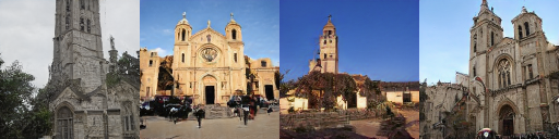
StyleGAN2-NoPathReg + RNI
StyleGAN2 + RNI

Figure 4: Synthesized images of different StyleGAN2-based models.

4.3 Geometric Realization of $\mu(x)$ and $\sigma(x)$

As $\mu$ stands for a particular point in the feature space, we simply model it by the traditional deep CNN architectures. $\sigma(x)$ is designed to fit the local geometry of $\mu(x)$. According to our theory, the local geometry should only admit minor differences from $\mu(x)$. Thus we believe that $\sigma(x)$ should be determined by the spatial and semantic information contained in $\mu(x)$, and should characterize the local variations of the spatial and semantic information. The deviation of pixel-wise sum along channels of feature maps in StyleGAN2 highlights the semantic variations like hair, parts of background, and silhouettes, as the standard deviation map over sampling instances shows in Fig. 1. This observation suggests that the sum along channels identifies the local semantics we expect to reveal. Thus it should be directly connected to $\sigma(x)$ we are pursuing here. For a given feature map $\mu=\mathbf{DCNN}(x)$ from the deep CNN, which is a specific point in the feature manifold, the sum along its channels is

$$\tilde{\mu}_{ijk}=\sum_{i=1}^{c}\mu_{ijk},\vspace{-0.2cm}$$ (13)

where $i$ enumerates all the $c$ feature maps of $\mu$, while $j,k$ enumerate the spatial footprint of $\mu$ in its $h$ rows and $w$ columns, respectively. The resulting $\tilde{\mu}$ is then a spatial semantic identifier, whose variation corresponds to the local semantic variation. We then normalize $\tilde{\mu}$ to obtain a spatial semantic coefficient matrix $s$ with

$$mean(\tilde{\mu}) =\frac{1}{h\times w}\sum_{j=1}^{h}\sum_{k=1}^{w}\tilde{\mu}_{jk},$$ (14)

$$s =\tilde{\mu}-mean(\tilde{\mu}),$$

$$max(|s|) =\max_{1\leq j\leq h,1\leq k\leq w}|s_{jk}|,$$

$$s =\frac{s}{max(|s|)}.$$

Recall that the standard deviation of $s$ over sampling instances highlights the local variance in semantics. Thus $s$ can be decomposed into two independent components: $s_{m}$ that corresponds to the main content of the output image, which is almost invariant under changes of injected noise; $s_{v}$ that is associated with the variance that is induced by the injected noise, and is nearly orthogonal to the main content. We assume that this decomposition can be attained by an affine transformation on $s$ such that

$$s_{d}=A*s+b=s_{m}+s_{v},s_{v}*\mu\approx\mathbf{0},\vspace{-0.15cm}$$ (15)

where $*$ denotes element-wise matrix multiplication, and $\mathbf{0}$ denotes the matrix whose all elements are zeros. To avoid numerical instability, we add $\mathbf{1}$ whose all elements are ones to the above decomposition, such that its condition number will not get exploded,

$$s^{\prime}=\alpha s_{d}+(1-\alpha)\mathbf{1},~{}\sigma=\frac{s^{\prime}}{\|s^{\prime}\|_{2}}.\vspace{-0.15cm}$$ (16)

The regularized $s_{m}$ component is then used to enhance the main content in $\mu$, and the regularized $s_{v}$ component is then used to guide the variance of injected noise. The final output $o$ is then calculated as

$$o=r\sigma*\mu+r\sigma*\epsilon,\epsilon\sim\mathcal{N}(0,1).\vspace{-0.15cm}$$ (17)

In the above procedure, $A,b,r,$ and $\alpha$ are learnable parameters. Note that in the last equation, we do not need to decompose $s^{\prime}$ into $s_{v}$ and $s_{m}$, as $s_{v}$ is designed to be nearly orthogonal to $\mu$, and $s_{m}$ is nearly invariant. Thus $\sigma*\mu$ will automatically drop the $s_{v}$ component, and $\sigma*\epsilon$ amounts to adding an invariant bias to the variance of injected noise. There are alternative forms for $\mu$ and $\sigma$ with respect to various GAN architectures. However, modeling $\mu$ by deep CNNs and deriving $\sigma$ through the spatial and semantic information of $\mu$ are universal for GANs, as they comply with our theorems. We further conduct an ablation study to verify the effectiveness of the above procedure. The related results can be found in the supplementary material.

Using our formulation, noise injection in StyleGAN2 can be written as follows:

$$\mu=\mathbf{DCNN}(x),o=\mu+r*\epsilon,~{}\epsilon\sim\mathcal{N}(0,1),\vspace{-0.15cm}$$ (18)

where $r$ is a learnable scalar parameter. This can be viewed as a special case of our method, where $T(\mu)$ in (11) is set to identity. Under this settings, the local geometry is assumed to be everywhere identical among the feature manifold, which suggests a globally Euclidean structure. While our theory supports this simplification and specialization, our choice of $\mu(x)$ and $\sigma(x)$ can suit broader and more usual occasions, where the feature manifolds are non-Euclidean. We denote this fashion of noise injection as Euclidean Noise Injection (ENI), and will extensively study its performance compared with our choice in the following section.

5 Experiment

We conduct experiments on benchmark datasets including FFHQ faces, LSUN objects, and CIFAR-10. The GAN models we use are the baseline DCGAN (Radford et al., 2015) (originally without noise injection) and the state-of-the-art StyleGAN2 (Karras et al., 2019b) (originally with Euclidean noise injection). For StyleGAN2, we use images of resolution $128\times 128$ and config-e in the original paper due to that config-e achieves the best performance with respect to Path Perceptual Length (PPL) score. Besides, we apply the experimental settings from StyleGAN2.

Noise injection presented in section 4.3 is called Riemannian Noise Injection (RNI) while the simple form used in StyleGAN is called Euclidean Noise Injection (ENI).

CIFAR-10
DCGAN	DCGAN + ENI	DCGAN + RNI
PPL=101.4,FID=83.8, IS=4.46	PPL=77.9, FID=84.8, IS=4.73	PPL=69.9, FID=83.2, IS=4.64
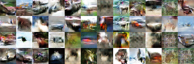
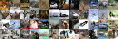
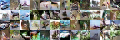
Cat-Selected
StyleGAN2 + ENI StyleGAN2 + RNI PPL=115, MC=0.725, TTMC=1.54 FID=12.7 PPL=106, MC=0.686, TTMC=1.45, FID=13.4

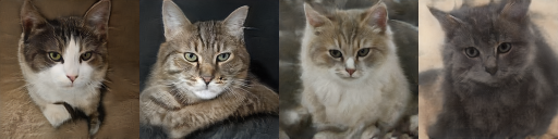
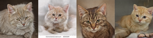
Figure 5: Image synthesis on CIFAR-10 and LSUN cats.

Image synthesis.

PPL (Zhang et al., 2018) has been proven an effective metric for measuring structural consistency of generated images (Karras et al., 2019b). Considering its similarity to the expectation of the Lipschitz constant of the generator, it can also be viewed as a quantification of the smoothness of the generator. The path length regularizer is proposed in StyleGAN2 to improve generated image quality by explicitly regularizing the Jacobian of the generator with respect to the intermediate latent space. We first compare the noise injection methods with the plain StyleGAN2, which remove the Euclidean noise injection and path length regularizer in StyleGAN2. As shown in Table 1, we can find that all types of noise injection significantly improve the PPL scores. It is worth noting that our method without path length regularizer can achieve comparable performance against the standard StyleGAN2 on the FFHQ dataset, and the performance can be further improved if combined with path length regularizer. Considering the extra GPU memory consuming of path length regularizer in training, we think that our method offers a computation-friendly alternative to StyleGAN2 as we observe smaller GPU memory occupation of our method throughout all the experiments.

For the LSUN-Church dataset, we observe an obvious improvement in FID scores compared with StyleGAN2. We believe that this is because the LSUN-Church data are scene images and contain various semantics of multiple objects, which are hard to fit for the original StyleGAN2 that is more suitable for single object synthesis. So our RNI architecture offers more degrees of freedom to the generator to fit the true distribution of the dataset. In all cases, our method is superior to StyleGAN2 in both PPL and FID scores. This proves that our noise injection method is more powerful than the one used in StyleGAN2. For DCGAN, as it does not possess the intermediate latent space, we cannot facilitate it with the path length regularizer. So we only compare the Euclidean noise injection with our RNI method. Through all the cases we can find that our method achieves the best performance in PPL and FID scores.

Table 2: Conditions for different GAN architectures. Lower condition metrics suggest better network stability and invertibility.

GAN arch	FFHQ		LSUN-Church
	MC ($\downarrow$)	TTMC ($\downarrow$)	MC ($\downarrow$)	TTMC ($\downarrow$)
Plain StyleGAN2	0.943	2.81	2.31	6.31
StyleGAN2 + ENI	0.666	1.27	0.883	1.75
StyleGAN2-NoPathReg + RNI (Ours)	0.766	2.39	1.71	4.74
StyleGAN2 + RNI (Ours)	0.530	1.05	0.773	1.51

We also study whether our choice for $\mu(x)$ and $\sigma(x)$ can be applied to broader occasions. We further conduct experiments on a cat dataset which consists of 100 thousand selected images from 800 thousand LSUN-Cat images by PageRank algorithm (Zhou et al., 2004). For DCGAN, we conduct extra experiments on CIFAR-10 to test whether our method could succeed in multi-class image synthesis. The results are reported in Figure 5. We can see that our method still outperforms the compared methods in PPL scores and the FID scores are comparable, indicating that the proposed noise injection is more favorable of preserving structural consistency of generated images with real ones.

Numerical stability.

As we have analyzed above, noise injection should be able to improve the numerical stability of GANs. To evaluate it, we examine the condition number of different GAN architectures. The condition number of a given function $f$ is defines as (Horn & Johnson, 2013)

$$C(f)=\limsup_{\|\Delta x\|\rightarrow 0}\frac{\|f(x)-f(x+\Delta x)\|/\|f(x)\|}{\|\Delta x\|/\|x\|}.\vspace{-0.15cm}$$ (19)

It measures how sensitive a function is to changes or errors in the input. A function with a high condition number is said to be ill-conditioned. Considering the numerical infeasibility of the $\sup$ operator in the definition of condition number, we resort to the following alternative approach. We first sample a batch of 50000 pairs of $(Input,Perturbation)$ from the input distribution and the perturbation $\Delta x\sim\mathcal{N}(0,1\text{e-}4)$, and then compute the corresponding condition numbers. We compute the mean value and the mean value of the largest 1000 values of these 50000 condition numbers as Mean Condition ($\mathbf{MC}$) and Top Thousand Mean Condition ($\mathbf{TTMC})$ respectively to evaluate the condition of GAN models. We report the results in Table 2, where we can find that noise injection significantly improves the condition of GAN models, and our proposed method dominates the performance.

GAN inversion.

StyleGAN2 makes use of a latent style space that is capable of enabling controllable image modifications. This characteristic motivates us to study the image embedding capability of our method via GAN inversion algorithms (Abdal et al., 2019) as it may help further leverage the potential of GAN models. From the experiments, we find that the StyleGAN2 model is prone to work well for full-face, non-blocking human face images. For this type of images, we observe comparable performance for all the GAN architectures. We think that this is because those images are close to the ‘mean’ face of FFHQ dataset (Karras et al., 2019a), thus easy to learn for the StyleGAN-based models. For faces of large pose or partially occluded ones, the capacity of compared models differs significantly. Noise injection methods outperform the plain StyleGAN2 by a large margin, and our method achieves the best performance. The detailed implementation and results are reported in the supplementary material.

6 Conclusion

In this paper, we propose a theoretical framework to explain the effect of noise injection technique in GANs. We prove that the generator can easily encounter the difficulty of nonsmoothness or expressiveness, and noise injection is an effective approach to addressing this issue. Based on our theoretical framework, we also derive a more proper formulation for noise injection. We conduct experiments on various datasets to confirm its validity. In future work, we will further investigate the universal realizations of noise injection for diverse GAN architectures, and attempt to find more powerful ways to characterize local geometries of feature spaces.

References

- Abdal et al. (2019) Abdal, R., Qin, Y., and Wonka, P. Image2StyleGAN: How to embed images into the StyleGAN latent space? In Proceedings of the IEEE International Conference on Computer Vision, pp. 4432–4441, 2019.
- An (1996) An, G. The effects of adding noise during backpropagation training on a generalization performance. Neural computation, 8(3):643–674, 1996.
- Arjovsky & Bottou (2017) Arjovsky, M. and Bottou, L. Towards principled methods for training generative adversarial networks. arxiv e-prints, art. arXiv preprint arXiv:1701.04862, 2017.
- Baskin et al. (2018) Baskin, C., Liss, N., Chai, Y., Zheltonozhskii, E., Schwartz, E., Giryes, R., Mendelson, A., and Bronstein, A. M. Nice: Noise injection and clamping estimation for neural network quantization. arXiv preprint arXiv:1810.00162, 2018.
- Bishop (1995) Bishop, C. M. Training with noise is equivalent to Tikhonov regularization. Neural computation, 7(1):108–116, 1995.
- Brock et al. (2018) Brock, A., Donahue, J., and Simonyan, K. Large-scale GAN training for high fidelity natural image synthesis, 2018.
- Chu et al. (2020) Chu, X., Zhang, B., and Li, X. Noisy differentiable architecture search. arXiv preprint arXiv:2005.03566, 2020.
- Goodfellow et al. (2014a) Goodfellow, I. J., Pouget-Abadie, J., Mirza, M., Xu, B., Warde-Farley, D., Ozair, S., Courville, A., and Bengio, Y. Generative adversarial networks, 2014a.
- Goodfellow et al. (2014b) Goodfellow, I. J., Shlens, J., and Szegedy, C. Explaining and harnessing adversarial examples. arXiv preprintarXiv:1412.6572, 2014b.
- He et al. (2019) He, Z., Rakin, A. S., and Fan, D. Parametric noise injection: Trainable randomness to improve deep neural network robustness against adversarial attack. In Proceedings of the IEEE Conference on Computer Vision and Pattern Recognition, pp. 588–597, 2019.
- Hinton et al. (2012) Hinton, G. E., Srivastava, N., Krizhevsky, A., Sutskever, I., and Salakhutdinov, R. R. Improving neural networks by preventing co-adaptation of feature detectors. arXiv preprint arXiv:1207.0580, 2012.
- Horn & Johnson (2013) Horn, R. A. and Johnson, C. R. Matrix Analysis. Cambridge University Press, 2013.
- Jenni & Favaro (2019) Jenni, S. and Favaro, P. On stabilizing generative adversarial training with noise. In Proceedings of the IEEE Conference on Computer Vision and Pattern Recognition, pp. 12145–12153, 2019.
- Karras et al. (2019a) Karras, T., Laine, S., and Aila, T. A style-based generator architecture for generative adversarial networks. In Proceedings of the IEEE Conference on Computer Vision and Pattern Recognition, pp. 4401–4410, 2019a.
- Karras et al. (2019b) Karras, T., Laine, S., Aittala, M., Hellsten, J., Lehtinen, J., and Aila, T. Analyzing and improving the image quality of StyleGAN. arXiv preprint arXiv:1912.04958, 2019b.
- Kingma & Welling (2013) Kingma, D. P. and Welling, M. Auto-encoding variational bayes. arXiv preprint arXiv:1312.6114, 2013.
- Ling & Bo (2003) Ling, Z. and Bo, Z. Theory of fuzzy quotient space (methods of fuzzy granular computing). 2003.
- Liu et al. (2019) Liu, H., Simonyan, K., and Yang, Y. Darts: Differentiable architecture search. International Conference of Representation Learning (ICLR), 2019.
- Murali (1989) Murali, V. Fuzzy equivalence relations. Fuzzy sets and systems, 30(2):155–163, 1989.
- Noh et al. (2017) Noh, H., You, T., Mun, J., and Han, B. Regularizing deep neural networks by noise: Its interpretation and optimization. Advances in Neural Information Processing Systems (NeurIPS), 2017.
- Petersen et al. (2006) Petersen, P., Axler, S., and Ribet, K. Riemannian geometry, volume 171. Springer, 2006.
- Radford et al. (2015) Radford, A., Metz, L., and Chintala, S. Unsupervised representation learning with deep convolutional generative adversarial networks. arXiv preprint arXiv:1511.06434, 2015.
- Recasens (2010) Recasens, J. Indistinguishability operators: Modelling fuzzy equalities and fuzzy equivalence relations, volume 260. Springer Science & Business Media, 2010.
- Roweis & Saul (2000) Roweis, S. T. and Saul, L. K. Nonlinear dimensionality reduction by locally linear embedding. Science, 290(5500):2323–2326, 2000.
- Rudin et al. (1964) Rudin, W. et al. Principles of mathematical analysis, volume 3. McGraw-hill New York, 1964.
- Srivastava et al. (2014) Srivastava, N., Hinton, G., Krizhevsky, A., Sutskever, I., and Salakhutdinov, R. Dropout: A simple way to prevent neural networks from overfitting. The journal of machine learning research, 15(1):1929–1958, 2014.
- Strang et al. (1993) Strang, G., Strang, G., Strang, G., and Strang, G. Introduction to linear algebra, volume 3. Wellesley-Cambridge Press Wellesley, MA, 1993.
- Tenenbaum et al. (2000) Tenenbaum, J. B., de Silva, V., and Langford, J. C. A global geometric framework for nonlinear dimensionality reduction. Science, 290(5500):2319–2323, 2000.
- Zhang et al. (2018) Zhang, R., Isola, P., Efros, A. A., Shechtman, E., and Wang, O. The unreasonable effectiveness of deep features as a perceptual metric. In Proceedings of the IEEE Conference on Computer Vision and Pattern Recognition, pp. 586–595, 2018.
- Zhou et al. (2004) Zhou, D., Weston, J., Gretton, A., Bousquet, O., and Schölkopf, B. Ranking on data manifolds. In Advances in neural information processing systems, pp. 169–176, 2004.