Chiral theory of nucleons and pions in the presence of an external gravitational field

Abstract

We extend the standard second order effective chiral Lagrangian of pions and nucleons by considering the coupling to an external gravitational field. As an application we calculate one-loop corrections to the one-nucleon matrix element of the energy-momentum tensor to fourth order in chiral counting, and next-to-leading order tree-level amplitude of the pion-production in an external gravitational field. We discuss the relation of the obtained results to experimentally measurable observables. Our expressions for the chiral corrections to the nucleon gravitational form factors differ from those in the literature. That might require to revisit the chiral extrapolation of the lattice data on the nucleon gravitational form factors obtained in the past.

I Introduction

Three basic global mechanical properties of the nucleon (mass, spin and the $D$-term) can be obtained as a linear response of the effective action to the change of the space-time metric. The mass, spin and $D$-term correspond to the hadron gravitational form factors (GFFs) at zero momentum transfer Kobzarev:1962wt ; Pagels:1966zza . While the mass and spin of the nucleon are well-studied and well-measured quantities, the third mechanical characteristics (the $D$-term) is more subtle, as it is related to the distribution of the internal forces inside the nucleon Polyakov:2002yz (for a review see Ref. Polyakov:2018zvc ). The nucleon gravitational form factors are measurable experimentally in exclusive processes like deeply virtual Compton scattering (DVCS) Ji:1996ek ; Radyushkin:1997ki and hard exclusive meson production Collins:1996fb .

The first results of measurements of the $D$-term in hard QCD processes became available in Refs. Kumericki:2015lhb ; Nature for the nucleon, and in Ref. Kumano:2017lhr for the pion. Profound studies of all subtleties in the extraction of the D-term from hard exclusive processes can be found in Ref. Kumericki:2019ddg . The GFFs have been also studied in lattice QCD, see Refs. Shanahan:2018nnv ; Shanahan:2018pib ; Alexandrou:2013joa ; Bratt:2010jn ; Hagler:2007xi and references therein.

The hard exclusive process can be used not only to access the GFFs of the nucleon, but also one can study other hadronic processes induced by the gravitational interaction. For example, the pion graviproduction off the nucleon Polyakov:1998sz ; Guichon:2003ah ; Polyakov:2006dd ; Kivel:2004bb .

For systematic studies of hadronic processes induced by gravity in the low-energy domain one needs to derive the Effective Chiral Lagrangian (EChL) for nucleons and pions in curved space-time. The corresponding EChL for pions has been derived in Ref. Donoghue:1991qv , and the GFFs of the pion obtained using EChL can be found in Ref. Kubis:1999db . In the present work we write down the full EChL of pions and nucleons in curved space-time up to second order. For that we couple the standard Lagrangian of chiral EFT up to order two Gasser:1984yg ; Fettes:2000gb to the gravitational field and introduce two additional terms which depend explicitly on the curvature characteristics of the space-time. Although these additional terms are zero in flat space-time, they contribute to the energy-momentum tensor (EMT) of pions and nucleons in Minkowski space-time and hence to GFFs of the nucleon as well as to hadronic processes induced by gravitational interaction.

In this work we apply the derived EChL to:

• manifestly Lorentz-invariant calculations of one-loop contributions to the nucleon gravitational form factors up to fourth order according to standard power counting rules. To remove the divergences and the power counting violating contributions from one-loop diagrams we apply the EOMS renormalization scheme of Refs. Gegelia:1999gf ; Fuchs:2003qc . We obtain the result which is at variance with the calculations of Ref. Diehl:2006ya done to the same chiral order using the heavy baryon formalism Jenkins:1990jv ; Bernard:1992qa . The origin of this difference was clarified with the authors of Ref. Diehl:2006ya - they agreed with our results. Our new expressions for the chiral corrections to nucleon GFFs might require revisiting the chiral extrapolation of the lattice data on these quantities obtained in the past.

• derivation of the large distance asymptotic of the energy, spin, pressure and shear force distributions in the parametrically wide region of distance $1/\Lambda_{\rm strong}\ll r\ll 1/M_{\pi}$.

• calculation of the amplitude of the pion graviproduction to next-to-leading order. The pion graviproduction can be accessed in hard exclusive processes Polyakov:1998sz ; Guichon:2003ah ; Polyakov:2006dd ; Kivel:2004bb and can be used to get additional information about the new low-energy constants of the EChL.

Surely, applications of the EChL derived here are not limited to the above physics problems. It can be used for a wide spectrum of applications, ranging from the physics of hadronic reactions in recently observed violent events, such as the neutron stars mergers TheLIGOScientific:2017qsa , to the fundamental questions of General Relativity (see, e.g., Ref. Avelino:2019esh ), and to the theory of hard exclusive processes and physics of exotic hadro-charmonia Dubynskiy:2008mq ; Eides:2015dtr ; Perevalova:2016dln .

Our paper is organized as follows: In section II we obtain the full second order EChL for pions and nucleons in curved space-time and the corresponding expression for EMT. Next we calculate the nucleon matrix element of the EMT in section III. The large distance asymptotic of the energy, spin, pressure and shear force distributions is studied in subsection III.1. In section IV we discuss the one-pion graviproduction tree-level amplitude at next-to-leading order. The results of our work are summarized in section V. The appendices contain definitions of loop integrals, explicit expressions of GFFs in the chiral limit, and the pion graviproduction amplitude.

II Effective action in curved space time and the energy-momentum tensor

In this section we obtain the full second order EChL for the pions and nucleons in curved space-time and derive the corresponding expression for the EMT. The EChL for pions and nucleons without including the coupling to gravitational fields can be found in Refs. Gasser:1984yg ; Fettes:2000gb . For the purpose of obtaining the EMT corresponding to these effective Lagrangians, analogously to Ref. Donoghue:1991qv , we consider their coupling to gravitational fields. The action corresponding to the leading order effective Lagrangian of pseudoscalar mesons interacting with the gravitational field is given by Donoghue:1991qv

$$S_{\rm\pi}=\int d^{4}x\sqrt{-g}\,\left\{\frac{F^{2}}{4}\,g^{\mu\nu}\,{\rm Tr}(D_{\mu}U(D_{\nu}U)^{\dagger})+\frac{F^{2}}{4}\,{\rm Tr}(\chi U^{\dagger}+U\chi^{\dagger})\right\},$$ (1)

where $\chi=2B_{0}(s+ip)$, $D_{\mu}U=\partial_{\mu}U-ir_{\mu}U+iUl_{\mu}$ and the $2\times 2$ unitary matrix $U$ represents the pion field. The parameter $B_{0}$ is related to the vacuum condensate and $s$, $p$, $l_{\mu}=v_{\mu}-a_{\mu}$ and $r_{\mu}=v_{\mu}+a_{\mu}$ are external sources.

For the action corresponding to the leading- and next-to-leading order effective Lagrangians of nucleons interacting with pions and the gravitational field we obtain:

$$S_{\rm\pi N} = \int d^{4}x\sqrt{-g}\,\biggl{\{}\frac{1}{2}\,\bar{\Psi}\,ie^{\mu}_{a}\gamma^{a}\nabla_{\mu}\Psi-\frac{1}{2}\,\nabla_{\mu}\bar{\Psi}\,ie^{\mu}_{a}\gamma^{a}\Psi-m\bar{\Psi}\Psi+\frac{g_{A}}{2}\,\bar{\Psi}e^{\mu}_{a}\gamma^{a}\gamma_{5}u_{\mu}\Psi$$ (2)

$$+ c_{1}\langle\chi_{+}\rangle\bar{\Psi}\Psi-\frac{c_{2}}{8m^{2}}g^{\mu\alpha}g^{\nu\beta}\langle u_{\mu}u_{\nu}\rangle\left(\bar{\Psi}\left\{\nabla_{\alpha},\nabla_{\beta}\right\}\Psi+\left\{\nabla_{\alpha},\nabla_{\beta}\right\}\bar{\Psi}\Psi\right)+\frac{c_{3}}{2}\,g^{\mu\nu}\langle u_{\mu}u_{\nu}\rangle\bar{\Psi}\Psi$$

$$+ \frac{ic_{4}}{4}\,\bar{\Psi}\,e^{\mu}_{a}e^{\nu}_{b}\sigma^{ab}\,\left[u_{\mu},u_{\nu}\right]\Psi+c_{5}\bar{\Psi}\hat{\chi}_{+}\Psi+\frac{c_{6}}{8m}\bar{\Psi}\,e^{\mu}_{a}e^{\nu}_{b}\sigma^{ab}F^{+}_{\mu\nu}\Psi+\frac{c_{7}}{8m}\bar{\Psi}\,e^{\mu}_{a}e^{\nu}_{b}\sigma^{ab}\langle F^{+}_{\mu\nu}\rangle\Psi$$

$$+ \frac{c_{8}}{8}\,R\bar{\Psi}\Psi+\frac{ic_{9}}{m}\,R^{\mu\nu}\left(\bar{\Psi}e_{\mu}^{a}\gamma_{a}\nabla_{\nu}\Psi-\nabla_{\nu}\bar{\Psi}e_{\mu}^{a}\gamma_{a}\Psi\right)\biggr{\}},$$

As usual, the action at this chiral order has been reduced to the above (minimal) form by using field redefinitions. In Eq. (2) $g^{\mu\nu}$ and $e^{\mu}_{a}$ are the metric (we use the signature $(+,-,-,-)$) and vielbein gravitational fields, respectively,

$$u_{\mu} = i\left[u^{\dagger}\partial_{\mu}u-u\partial_{\mu}u^{\dagger}-i(u^{\dagger}v_{\mu}u-uv_{\mu}u^{\dagger})\right]\,,$$

$$F_{\mu\nu}^{+} = u^{\dagger}F_{R\mu\nu}u+uF_{L\mu\nu}u^{\dagger}\,,$$

$$F_{R\mu\nu} = \partial_{\mu}r_{\nu}-\partial_{\nu}r_{\mu}-i[r_{\mu},r_{\nu}]\,,$$

$$F_{L\mu\nu} = \partial_{\mu}l_{\nu}-\partial_{\nu}l_{\mu}-i[l_{\mu},l_{\nu}]\,,$$

$$\chi_{+} = u^{\dagger}\chi u^{\dagger}+u\chi^{\dagger}u\,,$$

$$\hat{\chi}_{+} = \chi_{+}-\frac{1}{2}\langle\chi_{+}\rangle\,,$$ (3)

and the covariant derivative acting on the nucleon field has the form

$$\nabla_{\mu}\Psi = \partial_{\mu}\Psi+\frac{i}{2}\,\omega^{ab}_{\mu}\sigma_{ab}\Psi+\left(\Gamma_{\mu}-iv_{\mu}^{(s)}\right)\Psi,$$

$$\nabla_{\mu}\bar{\Psi} = \partial_{\mu}\bar{\Psi}-\frac{i}{2}\,\bar{\Psi}\,\sigma_{ab}\,\omega^{ab}_{\mu}-\bar{\Psi}\left(\Gamma_{\mu}-iv_{\mu}^{(s)}\right),$$ (4)

where $v_{\mu}^{(s)}$ is an iso-scalar external vector source, $\sigma_{ab}=\frac{i}{2}[\gamma_{a},\gamma_{b}]$ and

$$\Gamma_{\mu} = \frac{1}{2}\left[u^{\dagger}\partial_{\mu}u+u\partial_{\mu}u^{\dagger}-i(u^{\dagger}v_{\mu}u+uv_{\mu}u^{\dagger})\right]~{},$$

$$\omega_{\mu}^{ab} = -g^{\nu\lambda}e^{a}_{\lambda}\left(\partial_{\mu}e_{\nu}^{b}-e^{b}_{\sigma}\Gamma^{\sigma}_{\mu\nu}\right),$$

$$\Gamma^{\lambda}_{\alpha\beta} = \frac{1}{2}\,g^{\lambda\sigma}\left(\partial_{\alpha}g_{\beta\sigma}+\partial_{\beta}g_{\alpha\sigma}-\partial_{\sigma}g_{\alpha\beta}\right)~{},$$

$$R^{\rho}_{~{}\sigma\mu\nu} = \partial_{\mu}\Gamma^{\rho}_{\nu\sigma}-\partial_{\nu}\Gamma^{\rho}_{\mu\sigma}+\Gamma^{\rho}_{\mu\lambda}\Gamma^{\lambda}_{\nu\sigma}-\Gamma^{\rho}_{\nu\lambda}\Gamma^{\lambda}_{\mu\sigma}\,,$$

$$R = g^{\mu\nu}R^{\lambda}_{~{}\mu\lambda\nu}\,.$$ (5)

The vielbein fields satisfy the following relations:

$$e^{a}_{\mu}e^{b}_{\nu}\eta_{ab}=g_{\mu\nu},\ \ \ e_{a}^{\mu}e_{b}^{\nu}\eta^{ab}=g^{\mu\nu},$$

$$e^{a}_{\mu}e^{b}_{\nu}g^{\mu\nu}=\eta^{ab},\ \ \ e_{a}^{\mu}e_{b}^{\nu}g_{\mu\nu}=\eta_{ab}.$$ (6)

When calculating $\left\{\nabla_{\alpha},\nabla_{\beta}\right\}\Psi$ and $\left\{\nabla_{\alpha},\nabla_{\beta}\right\}\bar{\Psi}$ in Eq. (2) we need to take into account that the purely gravitational covariant derivative $\nabla^{\rm gr}_{\mu}$ acting on a tensor has the form:

$$\nabla^{\rm gr}_{\mu}T^{\alpha\beta\ldots}_{\rho\sigma\ldots}=\partial_{\mu}T^{\alpha\beta\ldots}_{\rho\sigma\ldots}+\Gamma^{\alpha}_{\mu\nu}T^{\nu\beta\ldots}_{\rho\sigma\ldots}+\ldots-\Gamma^{\nu}_{\mu\rho}T^{\alpha\beta\ldots}_{\nu\sigma\ldots}-\ldots\,.$$ (7)

The effective action of Eq. (2) contains low-energy constants (LECs), $c_{1-7}$ corresponding to the constants of the second order $\pi N$ effective action introduced in Ref. Fettes:2000gb , the values of which are constrained by data on low-energy physics of pions and nucleons. It also contains two new LECs, $c_{8}$ and $c_{9}$. We shall see below that they can be constrained by GFFs of the nucleon and/or by the pion graviproduction. It is important that these new LECs (like all others) are universal – the same constants enter various hadronic processes induced by gravity.

Using the definition of the EMT for matter fields interacting with the gravitational metric fields,

$$T_{\mu\nu}(g,\psi) = \frac{2}{\sqrt{-g}}\frac{\delta S_{\rm m}}{\delta g^{\mu\nu}}\,,$$ (8)

from the action of Eq. (1) we obtain in flat spacetime

$$T^{{(\pi)}}_{\mu\nu} = \frac{F^{2}}{4}\,{\rm Tr}(D_{\mu}U(D_{\nu}U)^{\dagger}+D_{\nu}U(D_{\mu}U)^{\dagger})-\eta_{\mu\nu}\left\{\frac{F^{2}}{4}\,{\rm Tr}(D^{\alpha}U(D_{\alpha}U)^{\dagger})+\frac{F^{2}}{4}\,{\rm Tr}(\chi U^{\dagger}+U\chi^{\dagger})\right\},$$ (9)

where $\eta_{\mu\nu}$ is the Minkowski metric tensor. For the fermion fields interacting with gravitational vielbein fields we use the definition Birrell:1982ix

$$T_{\mu\nu}(g,\psi) = \frac{1}{2e}\left[\frac{\delta S}{\delta e^{a\mu}}\,e^{a}_{\nu}+\frac{\delta S}{\delta e^{a\nu}}\,e^{a}_{\mu}\right],$$ (10)

where $e$ is the determinant of $e^{a}_{\mu}$. The action of Eq. (2) leads to the following expression for the EMT in flat spacetime:

$$T^{{(\pi N)}}_{\mu\nu} = \frac{i}{4}\,\left(\bar{\Psi}\,\gamma_{\mu}D_{\nu}\Psi+\bar{\Psi}\,\gamma_{\nu}D_{\mu}\Psi-D_{\mu}\bar{\Psi}\,\gamma_{\nu}\Psi-D_{\nu}\bar{\Psi}\,\gamma_{\mu}\Psi\right)+\frac{g_{A}}{4}\,\left(\bar{\Psi}\,\gamma_{\mu}\gamma_{5}u_{\nu}\Psi+\bar{\Psi}\,\gamma_{\nu}\gamma_{5}u_{\mu}\Psi\right)$$ (11)

$$- \frac{c_{2}}{8m^{2}}\left[\langle u_{\mu}u^{\beta}\rangle\left(\bar{\Psi}\left\{D_{\nu},D_{\beta}\right\}\Psi+\left\{D_{\nu},D_{\beta}\right\}\bar{\Psi}\Psi\right)+\langle u^{\alpha}u_{\mu}\rangle\left(\bar{\Psi}\left\{D_{\alpha},D_{\nu}\right\}\Psi+\left\{D_{\alpha},D_{\nu}\right\}\bar{\Psi}\Psi\right)\right.$$

$$+ \left.\langle u_{\nu}u^{\beta}\rangle\left(\bar{\Psi}\left\{D_{\mu},D_{\beta}\right\}\Psi+\left\{D_{\mu},D_{\beta}\right\}\bar{\Psi}\Psi\right)+\langle u^{\alpha}u_{\nu}\rangle\left(\bar{\Psi}\left\{D_{\alpha},D_{\mu}\right\}\Psi+\left\{D_{\alpha},D_{\mu}\right\}\bar{\Psi}\Psi\right)\right]$$

$$+ \frac{ic_{2}}{16m^{2}}\,\partial^{{\rho}}\left\{\langle u^{\alpha}u^{\beta}\rangle\left[D_{\alpha}\bar{\Psi}\left(\eta_{\beta\nu}\sigma_{{\rho}\mu}+\eta_{\beta\mu}\sigma_{{\rho}\nu}\right)\Psi+D_{\beta}\bar{\Psi}\left(\eta_{\alpha\nu}\sigma_{{\rho}\mu}+\eta_{\alpha\mu}\sigma_{{\rho}\nu}\right)\Psi\right]\right.$$

$$- \left.\langle u^{\alpha}u^{\beta}\rangle\left[\bar{\Psi}\left(\eta_{\beta\nu}\sigma_{{\rho}\mu}+\eta_{\beta\mu}\sigma_{{\rho}\nu}\right)D_{\alpha}\Psi+\bar{\Psi}\left(\eta_{\alpha\nu}\sigma_{{\rho}\mu}+\eta_{\alpha\mu}\sigma_{{\rho}\nu}\right)D_{\beta}\Psi\right]\right\}$$

$$+ \frac{c_{2}}{4m^{2}}\left\{\partial^{\alpha}\left[\langle u_{\alpha}u_{\mu}\rangle D_{\nu}(\bar{\Psi}\Psi)+\langle u_{\alpha}u_{\nu}\rangle D_{\mu}(\bar{\Psi}\Psi)-\langle u_{\mu}u_{\nu}\rangle D_{\alpha}(\bar{\Psi}\Psi)\right]\right\}$$

$$+ c_{3}\,\bar{\Psi}\langle u_{\mu}u_{\nu}\rangle\Psi+\frac{ic_{4}}{8}\bar{\Psi}\left(\sigma_{\nu\beta}\,\left[u_{\mu},u^{\beta}\right]+\sigma_{\alpha\nu}\,\left[u^{\alpha},u_{\mu}\right]+\sigma_{\mu\beta}\,\left[u_{\nu},u^{\beta}\right]+\sigma_{\alpha\mu}\,\left[u^{\alpha},u_{\nu}\right]\right)\Psi$$

$$+ \frac{c_{6}}{8m}\bar{\Psi}\left(\sigma_{\nu\beta}F^{+}_{\mu\alpha}\eta^{\alpha\beta}+\sigma_{\mu\beta}F^{+}_{\nu\alpha}\eta^{\alpha\beta}\right)\Psi+\frac{c_{7}}{8m}\bar{\Psi}\left(\sigma_{\nu\beta}\langle F^{+}_{\mu\alpha}\rangle\eta^{\alpha\beta}+\sigma_{\mu\beta}\langle F^{+}_{\nu\alpha}\rangle\eta^{\alpha\beta}\right)\Psi$$

$$+ \frac{c_{8}}{4}(\eta_{\mu\nu}\partial^{2}-\partial_{\mu}\partial_{\nu})\bar{\Psi}\Psi+\frac{ic_{9}}{2m}\,(\eta_{\mu\alpha}\eta_{\nu\beta}\partial^{2}+\eta_{\mu\nu}\partial_{\alpha}\partial_{\beta}-\eta_{\mu\alpha}\partial_{\nu}\partial_{\beta}-\eta_{\nu\alpha}\partial_{\mu}\partial_{\beta})$$

$$\times \left(\bar{\Psi}\gamma^{\alpha}D^{\beta}\Psi-D^{\beta}\bar{\Psi}\gamma^{\alpha}\Psi+\bar{\Psi}\gamma^{\beta}D^{\alpha}\Psi-D^{\alpha}\bar{\Psi}\gamma^{\beta}\Psi\right)$$

$$- \eta_{\mu\nu}\left[\frac{1}{2}\,\bar{\Psi}\,i\gamma^{\alpha}D_{\alpha}\Psi-\frac{1}{2}\,D_{\alpha}\bar{\Psi}\,i\gamma^{\alpha}\Psi-m\bar{\Psi}\Psi+\frac{g_{A}}{2}\,\bar{\Psi}\gamma^{\alpha}\gamma_{5}u_{\alpha}\Psi\right.$$

$$+ \left.c_{1}\langle\chi_{+}\rangle\bar{\Psi}\Psi-\frac{c_{2}}{8m^{2}}\langle u_{\alpha}u_{\beta}\rangle\left(\bar{\Psi}\left\{D^{\alpha},D^{\beta}\right\}\Psi+\left\{D^{\alpha},D^{\beta}\right\}\bar{\Psi}\Psi\right)+\frac{c_{3}}{2}\,\langle u_{\alpha}u^{\alpha}\rangle\bar{\Psi}\Psi+\frac{ic_{4}}{4}\,\bar{\Psi}\sigma^{\alpha\beta}\,\left[u_{\alpha},u_{\beta}\right]\Psi\right.$$

$$+ \left.c_{5}\bar{\Psi}\hat{\chi}_{+}\Psi+\frac{c_{6}}{8m}\bar{\Psi}\sigma^{\alpha\beta}F^{+}_{\alpha\beta}\Psi+\frac{c_{7}}{8m}\bar{\Psi}\sigma^{\alpha\beta}\langle F^{+}_{\alpha\beta}\rangle\Psi\right],$$

where

$$D_{\mu}\Psi = \partial_{\mu}\Psi+\left(\Gamma_{\mu}-iv_{\mu}^{(s)}\right)\Psi,$$

$$D_{\mu}\bar{\Psi} = \partial_{\mu}\bar{\Psi}-\bar{\Psi}\left(\Gamma_{\mu}-iv_{\mu}^{(s)}\right).$$ (12)

The expression of Eq. (11) can be used for calculations in the low-energy region of various matrix elements of the EMT (and of its various products with scalar, pseudoscalar, vector and axial-vector quark currents) between states containing one nucleon and an arbitrary number of pions. Below we apply Eq. (11) for calculations of the one-loop corrections to GFFs of the nucleon up to fourth chiral order, and of the pion graviproduction tree-level amplitude in the leading and next-to-leading chiral orders. The expression for the EMT of Eq. (11) can be also applied to variety of low-energy hadronic processes induced by gravity (by EMT) and to calculations of various corrections to GFFs.

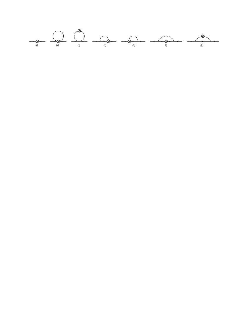
Figure 1: Tree and one-loop diagrams contributing to the nucleon matrix element of the EMT. Dashed and solid lines correspond to pions and nucleons, respectively. The circles with crosses represent the EMT vertices.

III One loop chiral corrections to nucleon gravitational form factors

In this section we calculate the tree and one-loop contributions to the nucleon matrix element of the EMT. The topologies of the corresponding diagrams are shown in Fig. 1. Standard power counting rules apply to these diagrams Weinberg:1991um ; Ecker:1994gg , i.e. the pion lines count as of chiral order minus two, the nucleon lines have order minus one, interaction vertices originating from the effective Lagrangian of order $N$ count also as of chiral order $N$ and the vertices generated by the EMT have the orders corresponding to the number of quark mass factors and derivatives acting on the pion fields, derivatives acting on the nucleon fields count as of chiral order zero. The momentum transfer between the initial and final nucleons also counts as of chiral order one, therefore in those terms of energy-momentum operator which contain full derivatives, these derivatives (although also acting on nucleon fields) count as of chiral order one. Integration over loop momenta is counted as of chiral order four.

Since we are interested in the nucleon matrix element of order four in the chiral expansion, we need vertices with two nucleon lines, generated by the EMT, up to order four. While we have obtained these vertices from the expression of Eq. (11) for zeroth, first and second chiral orders, for the third and fourth order terms we use a parameterisation as specified below. Simple power counting arguments show that, because the pion-nucleon-nucleon vertices have at least chiral order one, for all one-loop diagrams except f) we only need vertices up to order two. Naively it seems that for diagrams of topology f) we need also pion-nucleon-nucleon vertices of chiral order three, because the nucleon-nucleon vertex originating from the EMT starts with chiral order zero. However more careful examination reveals that the leading order contribution of the diagram with the mentioned zeroth order vertex is exactly canceled by the nucleon wave function renormalization constant multiplied by the tree order diagrams. Therefore the formally zeroth order vertex in effect starts contributing as a vertex of order one. As a result of this the diagram with the pion-nucleon-nucleon vertex of order three starts only contributing at chiral order five. For this reason we do not consider such diagrams in this work. Notice here that the above described power counting is realized in the results of our manifestly Lorentz-invariant calculations only after performing an appropriate renormalization.

The one-nucleon matrix element of the EMT is parameterised in terms of three form factors as follows Polyakov:2018zvc :

$$\langle p_{f},s_{f}|T_{\mu\nu}|p_{i},s_{i}\rangle = \bar{u}(p_{f},s_{f})\left[A(t)\frac{P_{\mu}P_{\nu}}{m_{N}}+iJ(t)\frac{P_{\mu}\sigma_{\nu\alpha}\Delta^{\alpha}+P_{\nu}\sigma_{\mu\alpha}\Delta^{\alpha}}{2m_{N}}+D(t)\frac{\Delta_{\mu}\Delta_{\nu}-\eta_{\mu\nu}q^{2}}{4m_{N}}\right]u(p_{i},s_{i})\,,$$ (13)

where $m_{N}$ is the physical mass of the nucleon, $(p_{i},s_{i})$ and $(p_{f},s_{f})$ are the momentum and polarization of the incoming and outgoing nucleons, respectively, and $P=(p_{i}+p_{f})/2$, $\Delta=p_{f}-p_{i}$, $t=\Delta^{2}$.

The tree-order diagrams up to chiral order four give the following contributions to the form factors:

$$A_{\rm tree}(t) = 1-\frac{2c_{9}}{m_{N}}\,t+x_{1}M_{\pi}^{2}t+x_{2}t^{2}\,,$$

$$J_{\rm tree}(t) = \frac{1}{2}-\frac{c_{9}}{m_{N}}\,t\,,$$

$$D_{\rm tree}(t) = c_{8}m_{N}+y_{1}t+y_{2}M_{\pi}^{2}\,.$$ (14)

where $c_{8}$ and $c_{9}$ terms are generated by the EMT of Eq. (11), while $x_{1}$ and $x_{2}$ ($y_{1}$ and $y_{2}$) parameterize the tree-order contributions of the fourth (the third) chiral orders. The parameters $x_{i}$ and $y_{i}$ are given as linear combinations of the coupling constants of the corresponding effective Lagrangians in the presence of the external gravitational field, derivation of which is beyond the scope of this work.

In calculations of loop diagrams, shown in Fig. 1 we applied dimensional regularization (see, e.g., Ref. Collins:1984xc ) and used the program FeynCalc Mertig:1990an ; Shtabovenko:2016sxi . The One-loop expressions of the form factors are too large to be shown explicitly. Instead we give the corresponding expressions in chiral limit in the appendix.

We perform the renormalization of loop diagrams by applying the EOMS scheme Gegelia:1999gf ; Fuchs:2003qc with the renormalization scale $\mu=m_{N}$. Notice that the divergent pieces of one-loop contributions to $A(t)$, as well as to $J(t)$, with coefficients of chiral orders zero and two, vanish. On the other hand there is a power counting violating contribution to $A(t)$ given by $3tg_{A}^{2}/(64\pi^{2}F^{2})$ which is absorbed into the renormalization of the coupling constant $c_{9}$ without affecting the power counting for $J(t)$ in which $c_{9}$ also gives a tree-order contribution. The coupling $c_{8}$ has to cancel the divergent part and the power counting violating piece of the one-loop contribution to $D(t)$ given by

$$-\frac{g_{A}^{2}}{16\pi^{2}F^{2}}\left[m_{N}^{2}B_{0}\left(m_{N}^{2},0,m_{N}^{2}\right)+\text{A}_{0}\left(m_{N}^{2}\right)\right]-\frac{3c_{8}g_{A}^{2}}{32\pi^{2}F^{2}}\left(2m_{N}^{3}-3m_{N}\text{A}_{0}\left(m_{N}^{2}\right)\right)+\frac{3c_{9}g_{A}^{2}m_{N}}{2\pi^{2}F^{2}}\text{A}_{0}\left(m_{N}^{2}\right)\,,$$ (15)

where the loop integrals $A_{0}$ and $B_{0}$ are defined in the appendix.

Adding the tree-order contribution of Eq. (14) to the one-loop result we obtain the following expression for the $D$-term $D(0)$ expanded in powers of the pion mass:

$$\frac{D(0)}{m_{N}} = c_{8}+\frac{g_{A}^{2}}{16\pi F^{2}}\,M_{\pi}+\frac{-3g_{A}^{2}/m_{N}+2\left(-4c_{1}+c_{2}+2c_{3}\right)}{8\pi^{2}F^{2}}\,M_{\pi}^{2}\ln\left(\frac{M_{\pi}}{m_{N}}\right)$$ (16)

$$+ \frac{\left(-g_{A}^{2}\left(3c_{8}+14/m_{N}\right)+8c_{3}-16c_{1}\right)}{32\pi^{2}F^{2}}\ M_{\pi}^{2}+\frac{y_{2}}{m_{N}}\ M_{\pi}^{2}+{\cal O}(M_{\pi}^{3})\,.$$

We notice that our result is at variance with calculations of Diehl et al. Diehl:2006ya done to the same chiral order using heavy baryon approach. More specifically our coefficients of the non-analytical $\sim M_{\pi}^{2}\ln(M_{\pi}/m_{N})$ terms proportional to LECs $c_{2,3}$ are different from those of Ref. Diehl:2006ya . For the remaining non-analytical contributions we found agreement with calculations of Ref. Diehl:2006ya and with other lower order calculations in Refs. Belitsky:2002jp ; Ando:2006sk ; Dorati:2007bk ; Moiseeva:2013qoa . Mentioned difference might lead to the revision of the extrapolation of lattice data of nucleon GFFs to the physical point.

Next we define the slopes of GFFs by writing the form factors as:

$$A(t) = 1+s_{A}t+{\cal O}(t^{2})\,,$$

$$J(t) = \frac{1}{2}+s_{J}t+{\cal O}(t^{2})\,,$$

$$D(t) = D(0)+s_{D}t+{\cal O}(t^{2})\,.$$ (17)

For the chiral expansion of the loop contributions to the slopes we obtain (while the tree-order contributions are included in Eq. (14) )

$$s_{A} = -\frac{7g_{A}^{2}}{128\pi F^{2}m_{N}}\ M_{\pi}+\frac{\left(c_{2}m_{N}-4g_{A}^{2}\right)}{16\pi^{2}F^{2}m_{N}^{2}}\ M_{\pi}^{2}\ln\left(\frac{M_{\pi}}{m_{N}}\right)-\frac{3g_{A}^{2}\left(2c_{9}m_{N}+1\right)}{32\pi^{2}F^{2}m_{N}^{2}}\ M_{\pi}^{2}+{\cal O}(M_{\pi}^{3})\,,$$

$$s_{J} = -\frac{g_{A}^{2}}{32\pi^{2}F^{2}}\ \ln\left(\frac{M_{\pi}}{m_{N}}\right)+\frac{g_{A}^{2}\left(4c_{9}m_{N}-5\right)}{64\pi^{2}F^{2}}+\frac{7g_{A}^{2}}{128\pi F^{2}m_{N}}\ M_{\pi}+{\cal O}(M_{\pi}^{2})\,,$$

$$s_{D} = -\frac{g_{A}^{2}m_{N}}{40\pi F^{2}}\ \frac{1}{M_{\pi}}-\frac{\left(5g_{A}^{2}+4\left(c_{2}+5c_{3}\right)m_{N}\right)}{80\pi^{2}F^{2}}\ \ln\left(\frac{M_{\pi}}{m_{N}}\right)+{\frac{g_{A}^{2}\left(24+(15c_{8}+40c_{9})m_{N}\right)}{480\pi^{2}F^{2}}}$$ (18)

$$+ \frac{\left(4c_{1}-c_{2}-7c_{3}\right)m_{N}}{40\pi^{2}F^{2}}+{\cal O}(M_{\pi})\,.$$

Again the non-analytic terms $\sim c_{2,3}M_{\pi}^{2}\ln(M_{\pi}/m_{N})$ in our calculation differ from those of Ref. Diehl:2006ya . For other non-analytical contributions we find agreement with calculations of Ref. Diehl:2006ya and with other lower order calculations in Refs. Belitsky:2002jp ; Ando:2006sk ; Dorati:2007bk ; Moiseeva:2013qoa .

III.1 Large distance asymptotics of the energy, spin, pressure and shear force distributions

The GFFs of the nucleon $A(t),J(t)$ and $D(t)$ can be related to the energy and spin densities as Polyakov:2002yz ; Polyakov:2018zvc :

$$\rho_{E}(r) = m_{N}\int\frac{d^{3}{\bf\Delta}}{(2\pi)^{3}}\ e^{{-i}{\bf r\Delta}}\,\biggl{[}A(-{\bf\Delta}^{2})+\frac{{\bf\Delta}^{2}}{4m_{N}^{2}}\bigl{[}A(-{\bf\Delta}^{2})-2J(-{\bf\Delta}^{2})+D(-{\bf\Delta}^{2})\bigr{]}\biggr{]}\,,$$ (19)

$$\rho_{J}(r) = \int\frac{d^{3}{\bf\Delta}}{(2\pi)^{3}}\ e^{{-i}{\bf r\Delta}}\,\left[J(-{\bf\Delta}^{2})+\frac{2}{3}{\bf\Delta}^{2}\frac{dJ(-{\bf\Delta}^{2})}{d{\bf\Delta}^{2}}\right]\,.$$ (20)

The vector field of the spin distribution in the polarised nucleon has the form $J^{i}({\bf r},{\bf s})=\frac{3}{2}\left(\delta^{ik}-\frac{r^{i}r^{k}}{r^{2}}\right)s^{k}\rho_{J}(r)$ Lorce:2017wkb ; Schweitzer:2019kkd . The distribution of the pressure $p(r)$ and shear force $s(r)$ are obtained through Polyakov:2002yz ; Polyakov:2018zvc :

$$s(r)=-\frac{1}{4m_{N}}\ r\frac{d}{dr}\frac{1}{r}\frac{d}{dr}{\widetilde{D}(r)},\quad p(r)=\frac{1}{6m_{N}}\frac{1}{r^{2}}\frac{d}{dr}r^{2}\frac{d}{dr}{\widetilde{D}(r)},\quad{\widetilde{D}(r)=}\int{\frac{d^{3}{\bf\Delta}}{(2\pi)^{3}}}\ e^{{-i}{\bf\Delta r}}\ D(-{\bf\Delta}^{2}).$$ (21)

The large distance power-like behavior of the distributions in the parametrically wide region $1/\Lambda_{\rm strong}\ll r\ll 1/M_{\pi}$ is governed by the singularities of GFFs at $t=0$, i.e. by the non-analytical terms of the GFFs in the chiral limit. From our loop calculations we can easily obtain the following small $t$ behavior of the GFFs in the chiral limit to the accuracy of our calculations:

$$A(t) = {1-\frac{2c_{9}}{m_{N}}\ t+\frac{3g_{A}^{2}}{512F^{2}m_{N}}(-t)^{\frac{3}{2}}-\frac{\left(c_{2}m_{N}-10g_{A}^{2}\right)}{320\pi^{2}F^{2}m_{N}^{2}}\ t^{2}\ln\left(\frac{-t}{m_{N}^{2}}\right)-\frac{\left(25g_{A}^{2}\left(12c_{9}m_{N}-7\right)-62c_{2}m_{N}\right)}{9600\pi^{2}F^{2}m_{N}^{2}}t^{2}}+{O(t^{\frac{5}{2}})}\,,$$

$$J(t) = {\frac{1}{2}-\frac{c_{9}}{m_{N}}\ t-\frac{g_{A}^{2}}{64\pi^{2}F^{2}}\ t\ln\left(\frac{-t}{m_{N}^{2}}\right)+{\frac{g_{A}^{2}\left(12c_{9}m_{N}-7\right)}{192\pi^{2}F^{2}}\ t}-\frac{3g_{A}^{2}}{512F^{2}m_{N}}}(-t)^{\frac{3}{2}}+{O(t^{2})}\,,$$

$$D(t) = {m_{N}c_{8}+\frac{3g_{A}^{2}m_{N}}{128F^{2}}\sqrt{-t}-\frac{\left(5g_{A}^{2}+4\left(c_{2}+5c_{3}\right)m_{N}\right)}{160\pi^{2}F^{2}}\ t\ln\left(\frac{-t}{m_{N}^{2}}\right)}$$ (22)

$$+ {\frac{\left(5g_{A}^{2}\left(40c_{9}m_{N}+15c_{8}m_{N}+28\right)+94c_{2}m_{N}+200c_{3}m_{N}\right)}{2400\pi^{2}F^{2}}\ t+{O(t^{\frac{3}{2}})}\,.}$$

Performing 3D Fourier transformation of these expressions we obtain the large distance behavior of the spatial distributions in the parametrically wide region $1/\Lambda_{\rm strong}\ll r\ll 1/M_{\pi}$:

$$\rho_{E}(r) = \frac{9g_{A}^{2}}{64\pi^{2}F^{2}}\frac{1}{r^{6}}{-\frac{3\left(10g_{A}^{2}/m_{N}+\left(c_{2}+10c_{3}\right)\right)}{16\pi^{3}F^{2}}\ \frac{1}{r^{7}}}+O\left(\frac{1}{r^{8}}\right)\,,$$ (23)

$$\rho_{J}(r) = {\frac{5g_{A}^{2}}{64\pi^{3}F^{2}}\frac{1}{r^{5}}-\frac{9g_{A}^{2}}{64\pi^{2}F^{2}m_{N}}\frac{1}{r^{6}}+O\left(\frac{1}{r^{7}}\right)}\,,$$ (24)

$$\widetilde{D}(r) = -\frac{3g_{A}^{2}m_{N}}{128\pi^{2}F^{2}}\frac{1}{r^{4}}+\frac{3\left(5g_{A}^{2}+4\left(c_{2}+5c_{3}\right)m_{N}\right)}{160\pi^{3}F^{2}}\ \frac{1}{r^{5}}+O\left(\frac{1}{r^{6}}\right)\,.$$ (25)

Using Eq. (25) in Eq. (21) we obtain the large distance behavior of the pressure and shear force distributions:

$$p(r) = -\frac{3g_{A}^{2}}{64\pi^{2}F^{2}}\frac{1}{r^{6}}{+\frac{\left(5g_{A}^{2}/m_{N}+4\left(c_{2}+5c_{3}\right)\right)}{16\pi^{3}F^{2}}\ \frac{1}{r^{7}}}+O\left(\frac{1}{r^{8}}\right),$$

$$s(r) = \frac{9g_{A}^{2}}{64\pi^{2}F^{2}}\frac{1}{r^{6}}{-\frac{21\left(5g_{A}^{2}/m_{N}+4\left(c_{2}+5c_{3}\right)\right)}{128\pi^{3}F^{2}}\ \frac{1}{r^{7}}}+O\left(\frac{1}{r^{8}}\right)\,.$$ (26)

The leading terms ($\sim 1/r^{6}$) in Eq. (26) have been obtained for the first time in Ref. Goeke:2007fp in the framework of the soliton picture of the nucleon. The obtained large distance asymptotics can be useful for the derivation of various inequalities for the bound states of various quarkonia with the nucleon in the hadro-quarkonium picture of the exotic pentaquarks with hidden heavy quarks content, see, e.g., Ref. Perevalova:2016dln . Also it can be useful for the analysis of lattice data on GFFs of the nucleon and for deriving general constraints on the GFFs. To illustrate the latter point we note that the large distance behavior of the energy density, given by Eq. (23), and of pressure and the shear force distributions, specified in Eq. (26), satisfy the general stability conditions - $\rho_{E}(r)>0$ and $\frac{2}{3}s(r)+p(r)>0$, see discussion in Ref. Polyakov:2018zvc .

Furthermore with help of expression for $J(t)$ in Eq. (22) we can obtain large impact-parameter behavior of the distributions of Belinfante-improved total angular momentum. The latter is defined as Lorce:2017wkb :

$$\langle J_{\rm Bel}\rangle(b_{\perp}) = -\frac{1}{2}b_{\perp}\frac{\partial}{\partial b_{\perp}}{\int\frac{d^{2}{\bf\Delta_{\perp}}}{(2\pi)^{2}}\ e^{{-i}{\bf b_{\perp}\Delta_{\perp}}}\,J(-{\bf\Delta_{\perp}}^{2})\,.}$$ (27)

Performing the 2D Fourier transformation we obtain the large $b_{\perp}$ asymptotics of $\langle J_{\rm Bel}\rangle(b_{\perp})$ as:

$$\langle J_{\rm Bel}\rangle(b_{\perp})=\frac{g_{A}^{2}}{16\pi^{3}F^{2}}\frac{1}{b_{\perp}^{4}}-\frac{135g_{A}^{2}}{2048\pi F^{2}m_{N}}\frac{1}{b_{\perp}^{5}}+O\left(\frac{1}{b_{\perp}^{6}}\right)\,.$$ (28)

This model-independent asymptotics is valid in the parametrically wide region $1/\Lambda_{\rm strong}\ll b_{\perp}\ll 1/M_{\pi}$ and can be used for derivation of model-independent constraints for total angular momentum distribution in the nucleon.

IV Pion graviproduction

The effective action of Eq. (2) obtained from the effective Lagrangian is universal and, hence, can be applied to a wide range of low-energy processes induced by gravity. As an example of an application of the action of Eq. (2) we consider in this section the tree-order amplitude of the one-pion production in a gravitational field close to threshold, where the chiral expansion of this quantity makes sense. The pion graviproduction is relevant not only for hadronic reactions in strong gravitational fields, but it can also be measured in hard exclusive processes Polyakov:1998sz ; Guichon:2003ah ; Polyakov:2006dd ; Kivel:2004bb .

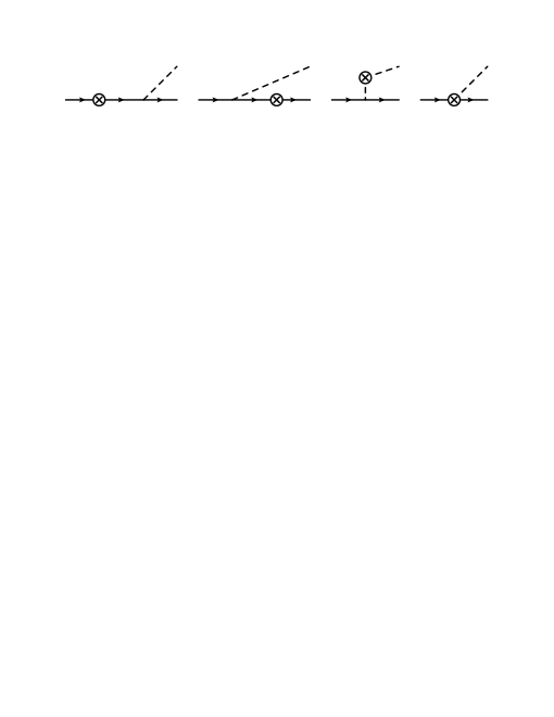
Figure 2: Tree-order diagrams contributing to the pion graviproduction. Dashed and solid lines correspond to pions and nucleons, respectively. The circles with crosses represent the EMT vertices.

The full tree-order amplitude of the one pion production ${\cal M}^{a,\mu\nu}=\langle\pi^{a}(k)N(p_{f})|T^{\mu\nu}(0)|N(p_{i})\rangle$ of leading and next-to-leading chiral orders is given in Eq. (33) of the appendix - the corresponding diagrams are shown in Fig. 2. Here we give the expression for the amplitude at threshold which can be parameterised in terms of GFFs for the $1/2^{+}\to 1/2^{-}$ transition. The corresponding form factors were introduced first in Ref. Kobzarev:1962wt for the case of equal masses of the final and initial states, for different masses they were considered in Ref. MVPAT . Following the latter reference we obtain the threshold amplitude of the pion graviproduction in the following form:

$$-i\ {\cal M}_{\rm tree}^{a,\mu\nu} = F_{1}({\Delta^{2}})\,\bar{u}(p_{f})\frac{\tau^{a}}{2}\left\{\,\Delta^{2}P^{\mu}P^{\nu}-(m_{*}^{2}-m_{N}^{2})\Delta^{\{\mu}P^{\nu\}}+\frac{(m_{*}^{2}-m_{N}^{2})^{2}}{4}\,g^{\mu\nu}\right\}\gamma^{5}u(p_{i})$$ (29)

$$+ F_{2}({\Delta^{2}})\,\bar{u}(p_{f})\frac{\tau^{a}}{2}\left\{\,\Delta^{2}\gamma^{\{\mu}P^{\nu\}}-(m_{*}+m_{N})\Delta^{\{\mu}P^{\nu\}}-\frac{(m_{*}^{2}-m_{N}^{2})}{2}\,\left(\gamma^{\{\mu}\Delta^{\nu\}}-(m_{*}+m_{N})g^{\mu\nu}\right)\right\}\gamma^{5}u(p_{i})$$

$$+ F_{3}({\Delta^{2}})\,\left\{\,\Delta^{\mu}\Delta^{\nu}-g^{\mu\nu}\Delta^{2}\right\}\bar{u}(p_{f})\frac{\tau^{a}}{2}\gamma^{5}u(p_{i})\,,$$

where $\Delta=p_{f}+k-p_{i}$, $P=p_{i}+\frac{\Delta}{2}$, $m_{*}=m_{N}+M_{\pi}$, and the symmetrization is defined as $X^{\{\mu}Y^{\nu\}}=(X^{\mu}Y^{\nu}+X^{\nu}Y^{\mu})/2$.

Our tree order calculation gives:

$$F_{1}({\Delta^{2}}) = \frac{8\,c_{9}g_{A}m_{N}}{F{m_{*}}\left(m_{N}\left(m_{*}+m_{N}\right)-{\Delta^{2}}\right)}+\frac{4g_{A}m_{N}\left(m_{N}-M_{\pi}\right)}{F\left(m_{N}\left(m_{*}+m_{N}\right)-{\Delta^{2}}\right)\left(M_{\pi}^{2}\left(m_{*}+m_{N}\right)-{\Delta^{2}}m_{N}\right)}\,,$$

$$F_{2}({\Delta^{2}}) = \frac{2g_{A}m_{N}}{F\left({m_{*}+m_{N}}\right)\left(m_{N}\left({{m_{*}}}+m_{N}\right)-{\Delta^{2}}\right)}-\frac{2\,c_{9}g_{A}\left(M_{\pi}m_{N}\left({m_{*}}+m_{N}\right){}^{2}+{\Delta^{2}}\left(2m_{N}^{2}-M_{\pi}^{2}\right)\right)}{F{m_{*}}m_{N}\left({m_{*}+m_{N}}\right)\left(m_{N}\left({m_{*}}+m_{N}\right)-{\Delta^{2}}\right)}\,,$$

$$F_{3}({\Delta^{2}}) = -\frac{c_{9}M_{\pi}g_{A}\left(-M_{\pi}^{2}m_{N}+4m_{N}^{3}+M_{\pi}{\Delta^{2}}\right)}{Fm_{*}m_{N}\left(m_{N}\left(m_{*}+m_{N}\right)-{\Delta^{2}}\right)}-\frac{c_{8}m_{*}g_{A}\left(2m_{N}\left(m_{*}+m_{N}\right)-{\Delta^{2}}\right)}{2F\left(m_{*}+m_{N}\right)\left(m_{N}\left(m_{*}+m_{N}\right)-{\Delta^{2}}\right)}$$ (30)

$$+ \frac{M_{\pi}g_{A}m_{N}\left(-4m_{N}^{2}+M_{\pi}^{2}+{\Delta^{2}}\right)}{F\left(m_{N}\left(m_{*}+m_{N}\right)-{\Delta^{2}}\right)\left(M_{\pi}^{2}\left(m_{*}+m_{N}\right)-{\Delta^{2}}m_{N}\right)}\,.$$

In the momentum transfer range ${\Delta^{2}}\sim M_{\pi}^{2}\sim\varepsilon^{2}\to 0$ the above form factors scale as $F_{1}({\Delta^{2}})\sim 1/\varepsilon^{2}$, $F_{2}({\Delta^{2}})\sim\varepsilon^{0}$, and $F_{3}({\Delta^{2}})\sim 1/\varepsilon$.

Our amplitude of the pion graviproduction (see the above equation and Eq. (33) in the appendix) depends on the new LECs $c_{8}$ and $c_{9}$. Therefore the measurements of the pion graviproduction process can be used as an additional source of information on these LECs, and also for studying the applicability of the chiral effective field theory to reactions induced by gravitational interactions. The pion graviproduction can be accessed in hard exclusive processes like the non-diagonal DVCS ($\gamma^{*}+N\to\gamma+(\pi N)$) Polyakov:1998sz ; Guichon:2003ah ; Polyakov:2006dd ; Kivel:2004bb . The corresponding measurements are planned by the CLAS12 collaboration at JLab (USA) privatcomm .

V Summary

In the current work we presented the effective chiral Lagrangian of pions and nucleons up to the second chiral order in the presence of external gravitational field. We derived the corresponding energy-momentum tensor of pions and nucleons (with external scalar, pseudoscalar, vector and axial-vector quark currents included) in flat space-time. Next we calculated the one-loop contributions to the one-nucleon matrix element of the energy-momentum tensor at fourth chiral order and extracted the corresponding contributions to gravitational form factors of the nucleon. To renormalize the loop diagrams we applied the EOMS renormalization scheme of Refs. Gegelia:1999gf ; Fuchs:2003qc . For the tree contributions of the first and the second order we obtained the Feynman rules from the corresponding expressions of the energy-momentum tensor while for the third and fourth orders we used parametrizations in most general form. While the coefficients of these parametrizations can be expressed as linear combinations of the coupling constants of the effective Lagrangians of the corresponding chiral orders in the presence of an external gravitational field, derivation of these Lagrangians and the corresponding energy-momentum tensors is beyond the scope of this work. As the obtained expressions for the gravitational form factors of the nucleon, defined by the matrix element of the energy-momentum tensor, are too large to be given explicitly, in the appendix we quote them in the chiral limit. We calculated the chiral expansion of the $D(0)$ and slope parameters for all GFFs to the fourth order of the chiral expansion. Our results for non-analytical contributions of the type $\sim c_{2,3}M_{\pi}^{2}\ln(M_{\pi}/m_{N})$ differ from those of the previous fourth order calculations of Ref. Diehl:2006ya . For the remaining non-analytical contributions we found agreement with the calculations of Ref. Diehl:2006ya and with other lower order calculations in Refs. Belitsky:2002jp ; Ando:2006sk ; Dorati:2007bk ; Moiseeva:2013qoa . The difference of our results with those in Ref. Diehl:2006ya was discussed with the authors of Ref. Diehl:2006ya and they agreed with our calculations. It is very important to check how strong the new results affect the chiral extrapolation of the lattice data on nucleon GFFs obtained in the past. However this is beyond the scope of the current work.

Furthermore we calculated the leading- and next-to-leading order tree contributions to the amplitude of the pion graviproduction. The process of the pion graviproduction provides an additional independent (to gravitational form factors) source of information on the new LECs $c_{8,9}$. It also offers a test of applicability of chiral perturbation theory to gravity-induced low-energy processes. Possibility of measurements of the pion graviproduction in hard exclusive processes has been discussed in Refs. Polyakov:1998sz ; Guichon:2003ah ; Polyakov:2006dd ; Kivel:2004bb . Such kind of experiments are planned by the CLAS12 collaboration at JLab (USA) privatcomm . The effective action of Eq. (2) obtained here provides a systematic tool of analyzing the data on these processes.

Appendix A Definition of loop integrals

The one-loop integrals appearing in expressions of our quoted results are defined as follows:

$$A_{0}(m^{2}) = \frac{(2\pi)^{4-n}}{i\pi^{2}}\int\frac{d^{n}k}{k^{2}-m^{2}+i\epsilon}\,,$$

$$B_{0}(p^{2},m_{1}^{2},m_{2}^{2}) = \frac{(2\pi)^{4-n}}{i\pi^{2}}\int\frac{d^{n}k}{[k^{2}-m_{1}^{2}+i\epsilon][(p+k)^{2}-m_{2}^{2}+i\epsilon]}\,,$$

$$C_{0}(p_{1}^{2},p_{2}^{2},p^{2}_{12},m_{1}^{2},m_{2}^{2},m_{3}^{2}) = \frac{(2\pi)^{4-n}}{i\pi^{2}}\int\frac{d^{n}k}{[k^{2}-m_{1}^{2}+i\epsilon][(p_{1}+k)^{2}-m_{2}^{2}+i\epsilon][(p_{1}+p_{2}+k)^{2}-m_{3}^{2}+i\epsilon]}\,,$$ (31)

with $p_{12}=p_{1}+p_{2}$. For the reduction of tensor loop integrals to scalar ones we apply the formulae specified in Ref. Denner:2005nn while for the expansion in terms of kinematical invariants we use Ref. Devaraj:1997es .

Appendix B One-loop expressions for form factors in chiral limit

Renormalized expressions of form factors in chiral limit for $\mu=m_{N}$:

$$A(t) = 1-\frac{2c_{9}t}{m_{N}}+\frac{tg_{A}^{2}}{64\pi^{2}F^{2}\left(4m_{N}^{2}-t\right){}^{3}}\biggl{[}-48tm_{N}^{4}\left(m_{N}^{2}+t\right)\text{C}_{0}\left(m_{N}^{2},m_{N}^{2},t,0,m_{N}^{2},0\right)$$

$$-2m_{N}^{2}\left(t-4m_{N}^{2}\right){}^{2}B_{0}\left(t,m_{N}^{2},m_{N}^{2}\right)-4tm_{N}^{2}B_{0}(t,0,0)\left(26m_{N}^{2}+t\right)-42t^{2}m_{N}^{2}+248tm_{N}^{4}-32m_{N}^{6}+3t^{3}\biggr{]}$$

$$+\frac{c_{9}t^{2}g_{A}^{2}m_{N}\left(B_{0}\left(t,m_{N}^{2},m_{N}^{2}\right)-1\right)}{16\pi^{2}F^{2}\left(4m_{N}^{2}-t\right)}+\frac{c_{2}t^{2}\left(15B_{0}(t,0,0)+16\right)}{4800\pi^{2}F^{2}m_{N}}\,,$$

$$J(t) = \frac{1}{2}-\frac{c_{9}t}{m_{N}}+\frac{g_{A}^{2}}{128\pi^{2}F^{2}\left(t-4m_{N}^{2}\right){}^{2}}\biggl{[}24t^{2}m_{N}^{4}\text{C}_{0}\left(m_{N}^{2},m_{N}^{2},t,0,m_{N}^{2},0\right)+4tm_{N}^{2}B_{0}(t,0,0)\left(8m_{N}^{2}+t\right)$$

$$+2\left(tm_{N}-4m_{N}^{3}\right){}^{2}B_{0}\left(t,m_{N}^{2},m_{N}^{2}\right)+30t^{2}m_{N}^{2}-128tm_{N}^{4}+32m_{N}^{6}-3t^{3}\biggr{]}-\frac{c_{9}tg_{A}^{2}m_{N}\left(B_{0}\left(t,m_{N}^{2},m_{N}^{2}\right)-1\right)}{32\pi^{2}F^{2}}\,,$$

$$D(t) = m_{N}c_{8}+\frac{g_{A}^{2}m_{N}^{2}}{48\pi^{2}F^{2}t\left(t-4m_{N}^{2}\right){}^{2}}\biggl{[}6m_{N}^{2}\left(3t^{2}\left(2m_{N}^{2}-t\right)\text{C}_{0}\left(m_{N}^{2},m_{N}^{2},t,0,m_{N}^{2},0\right)-2\left(t-4m_{N}^{2}\right){}^{2}B_{0}\left(t,m_{N}^{2},m_{N}^{2}\right)\right)$$ (32)

$$+6t^{2}B_{0}(t,0,0)\left(m_{N}^{2}-t\right)-22t^{2}m_{N}^{2}+128tm_{N}^{4}-192m_{N}^{6}+5t^{3}\biggr{]}+\frac{3c_{8}g_{A}^{2}m_{N}^{3}\left(B_{0}\left(t,m_{N}^{2},m_{N}^{2}\right)+1\right)}{16\pi^{2}F^{2}}$$

$$+\frac{c_{9}g_{A}^{2}m_{N}^{3}\left(B_{0}\left(t,m_{N}^{2},m_{N}^{2}\right)+1\right)}{2\pi^{2}F^{2}}+\frac{c_{2}t\left(15B_{0}(t,0,0)\left(8m_{N}^{2}+3t\right)+68m_{N}^{2}-42t\right)}{4800\pi^{2}F^{2}m_{N}}$$

$$+\frac{c_{3}tm_{N}\left(3B_{0}(t,0,0)-1\right)}{24\pi^{2}F^{2}}\,.$$

Appendix C Tree-order amplitude of the one-pion production

Tree-order amplitude of the pion production ${\cal M}^{a,\mu\nu}=\langle\pi^{a}(k)N(p_{f})|T^{\mu\nu}(0)|N(p_{i})\rangle$ has the following form:

$$-i\ {\cal M}_{\rm tree}^{a,\mu\nu} = \bar{u}(p_{f},s_{f})\frac{\tau^{a}}{2}\Biggl{\{}\,\frac{g_{A}}{2F\left(m_{N}^{2}-s\right)}\left(c_{8}m_{N}\left(q^{2}g^{\mu\nu}-q^{\mu}q^{\nu}\right)\not k\gamma^{5}+\left(m_{N}-2c_{9}q^{2}\right)\left(\left(2\ {p_{i}^{\nu}}+q^{\nu}\right)\not k\gamma^{\mu}\gamma^{5}\right.\right.$$ (33)

$$+ \left.\left.\left(2\ {p_{i}^{\mu}}+q^{\mu}\right)\not k\gamma^{\nu}\gamma^{5}\right)\right)+\frac{g_{A}}{2F\left(m_{N}^{2}-u\right)}\left(c_{8}m_{N}\left(q^{2}g^{\mu\nu}-q^{\mu}q^{\nu}\right)\not k\gamma^{5}+\left(2c_{9}q^{2}-m_{N}\right)\left(\left(2p_{f}^{\nu}-q^{\nu}\right)\gamma^{\mu}\not k\gamma^{5}\right.\right.$$

$$+ \left.\left.\left(2p_{f}^{\mu}-q^{\mu}\right)\gamma^{\nu}\not k\gamma^{5}\right)\right)+\frac{g_{A}m_{N}}{F\left(M_{\pi}^{2}-t\right)}\,\gamma^{5}\left(q^{2}g^{\mu\nu}+4\text{{k}}^{\mu}\text{{k}}^{\nu}-2q^{\nu}\text{{k}}^{\mu}-2q^{\mu}\text{{k}}^{\nu}\right)$$

$$- \frac{c_{9}g_{A}}{2Fm_{N}}\left(2\left(q^{2}-t\right)g^{\mu\nu}\not k\gamma^{5}-2\left(q^{\nu}\text{{k}}^{\mu}+q^{\mu}\text{{k}}^{\nu}\right)\left(\not k\gamma^{5}-2\gamma^{5}m_{N}\right)+\gamma^{\mu}\gamma^{5}\left(2q^{2}\text{{k}}^{\nu}+q^{\nu}\left(t-q^{2}\right)\right)\right.$$

$$+ \left.\gamma^{\nu}\gamma^{5}\left(2q^{2}\text{{k}}^{\mu}+q^{\mu}\left(t-q^{2}\right)\right)\right)+\frac{c_{9}M_{\pi}^{2}g_{A}}{2Fm_{N}}\left(-2g^{\mu\nu}\not k\gamma^{5}+\gamma^{\mu}\gamma^{5}q^{\nu}+\gamma^{\nu}\gamma^{5}q^{\mu}\right)$$

$$+ \frac{c_{8}g_{A}}{2F}\gamma^{5}\left(q^{2}g^{\mu\nu}-q^{\mu}q^{\nu}\right)+\frac{g_{A}m_{N}}{F}\,\gamma^{5}g^{\mu\nu}\Biggr{\}}u(p_{i},s_{i})\,,$$

where $q=p_{f}+k-p_{i}$ and the Mandelstam variables $s,t,u$ are defined as: $s=(p_{f}+k)^{2},t=(p_{f}-p_{i})^{2},u=(k-p_{i})^{2}$. One can easily check that the obtained amplitude is explicitly transverse, i.e. $q_{\mu}{\cal M}^{a,\mu\nu}=q_{\nu}{\cal M}^{a,\mu\nu}=0$ as it follows from conservation of EMT.

References

• (1) M. V. Polyakov and C. Weiss, “Skewed and double distributions in pion and nucleon,” Phys. Rev. D 60 (1999) 114017, [hep-ph/9902451].
• (2) I. Y. Kobzarev and L. B. Okun, Zh. Eksp. Teor. Fiz.  43, 1904 (1962) [Sov. Phys. JETP 16, 1343 (1963)].
• (3) H. Pagels, Phys. Rev.  144, 1250 (1966).
• (4) M. V. Polyakov, Phys. Lett. B 555, 57 (2003), [hep-ph/0210165].
• (5) M. V. Polyakov and P. Schweitzer, Int. J. Mod. Phys. A 33, no. 26, 1830025 (2018), [arXiv:1805.06596 [hep-ph]].
• (6) X. D. Ji, Phys. Rev. Lett. 78 (1997), 610-613, [arXiv:hep-ph/9603249 [hep-ph]].
• (7) A. Radyushkin, Phys. Rev. D 56, 5524-5557 (1997), [arXiv:hep-ph/9704207 [hep-ph]].
• (8) J. C. Collins, L. Frankfurt and M. Strikman, Phys. Rev. D 56, 2982-3006 (1997), [arXiv:hep-ph/9611433 [hep-ph]].
• (9) K. Kumericki and D. Mueller, “Description and interpretation of DVCS measurements,” EPJ Web Conf.  112 (2016) 01012, [arXiv:1512.09014 [hep-ph]].
• (10) V. D. Burkert, L. Elouadrhiri and F. X. Girod, Nature 557 (2018), 396.
• (11) S. Kumano, Q. T. Song and O. V. Teryaev, Phys. Rev. D 97 (2018), 014020, [arXiv:1711.08088 [hep-ph]].
• (12) K. Kumericki, Nature 570 (2019) no.7759, E1-E2.
• (13) P. Shanahan and W. Detmold, Phys. Rev. Lett. 122 (2019) no.7, 072003, [arXiv:1810.07589 [nucl-th]].
• (14) P. Shanahan and W. Detmold, Phys. Rev. D 99 (2019) no.1, 014511, [arXiv:1810.04626 [hep-lat]].
• (15) C. Alexandrou, M. Constantinou, S. Dinter, V. Drach, K. Jansen, C. Kallidonis and G. Koutsou, Phys. Rev. D 88 (2013) no.1, 014509, [arXiv:1303.5979 [hep-lat]].
• (16) J. Bratt et al. [LHPC], Phys. Rev. D 82 (2010), 094502, [arXiv:1001.3620 [hep-lat]].
• (17) P. Hagler et al. [LHPC], Phys. Rev. D 77 (2008), 094502, [arXiv:0705.4295 [hep-lat]].
• (18) M. V. Polyakov, “$N\to\Delta$ and $N\to N\pi$ DVCS and skewed quark distributions,” Proceedings of 8th International Conference on the Structure of Baryons (Baryons 98), Bonn, Germany, 22-26 Sep 1998, pp. 765-769.
• (19) P. A. Guichon, L. Mossé and M. Vanderhaeghen, Phys. Rev. D 68 (2003), 034018, [arXiv:hep-ph/0305231 [hep-ph]].
• (20) M. V. Polyakov and S. Stratmann, “Soft Pion Emission in Hard Exclusive Pion Production,” [arXiv:hep-ph/0609045 [hep-ph]].
• (21) N. Kivel, M. Polyakov and S. Stratmann, “Soft pion emission from the nucleon induced by twist-2 light-cone operators,” [arXiv:nucl-th/0407052 [nucl-th]].
• (22) J. F. Donoghue and H. Leutwyler, Z. Phys. C 52, 343 (1991).
• (23) B. Kubis and U.-G. Meißner, Nucl. Phys. A 671 (2000), 332-356, [arXiv:hep-ph/9908261 [hep-ph]].
• (24) J. Gasser and H. Leutwyler, Ann. Phys. (N.Y.) 158, 142 (1984).
• (25) N. Fettes, U.-G. Meißner, M. Mojžiš, and S. Steininger, Ann. Phys. (N.Y.) 283, 273 (2000); 288, 249 (2001).
• (26) J. Gegelia and G. Japaridze, Phys. Rev. D 60, 114038 (1999), [arXiv:hep-ph/9908377 [hep-ph]].
• (27) T. Fuchs, J. Gegelia, G. Japaridze and S. Scherer, Phys. Rev. D 68, 056005 (2003).
• (28) M. Diehl, A. Manashov and A. Schäfer, Eur. Phys. J. A 29, 315 (2006), [hep-ph/0608113].
• (29) E. E. Jenkins and A. V. Manohar, Phys. Lett. B 255, 558 (1991).
• (30) V. Bernard, N. Kaiser, J. Kambor and U.-G. Meißner, Nucl. Phys. B 388, 315 (1992).
• (31) B. P. Abbott et al. [LIGO Scientific and Virgo Collaborations], “GW170817: Observation of Gravitational Waves from a Binary Neutron Star Inspiral,” Phys. Rev. Lett.  119 (2017) no.16, 161101, [arXiv:1710.05832 [gr-qc]].
• (32) P. Avelino, Phys. Lett. B 795 (2019), 627-631, [arXiv:1902.01318 [gr-qc]].
• (33) S. Dubynskiy and M. Voloshin, Phys. Lett. B 666 (2008), 344-346, [arXiv:0803.2224 [hep-ph]].
• (34) M. I. Eides, V. Y. Petrov and M. V. Polyakov, Phys. Rev. D 93 (2016) no.5, 054039, [arXiv:1512.00426 [hep-ph]].
• (35) I. Perevalova, M. Polyakov and P. Schweitzer, Phys. Rev. D 94 (2016) no.5, 054024, [arXiv:1607.07008 [hep-ph]].
• (36) M. Dorati, T. A. Gail and T. R. Hemmert, Nucl. Phys. A 798 (2008), 96-131, [arXiv:nucl-th/0703073 [nucl-th]].
• (37) N. D. Birrell and P. C. W. Davies, “Quantum Fields in Curved Space,” Cambridge Univ. Press, Cambridge, UK, 1984.
• (38) S. Weinberg, Nucl. Phys. B 363, 3-18 (1991).
• (39) G. Ecker, Prog. Part. Nucl. Phys. 35, 1-80 (1995), [arXiv:hep-ph/9501357 [hep-ph]].
• (40) J. C. Collins, Renormalization (Cambridge University Press, Cambridge, UK, 1984).
• (41) R. Mertig, M. Bohm and A. Denner, Comput. Phys. Commun.  64, 345 (1991).
• (42) V. Shtabovenko, R. Mertig and F. Orellana, Comput. Phys. Commun.  207 (2016) 432
• (43) S. I. Ando, J. W. Chen and C. W. Kao, Phys. Rev. D 74 (2006), 094013, [arXiv:hep-ph/0602200 [hep-ph]].
• (44) A. Moiseeva and A. Vladimirov, Few Body Syst. 55 (2014), 389-394, [arXiv:1311.3433 [hep-ph]].
• (45) A. V. Belitsky and X. Ji, Phys. Lett. B 538, 289 (2002), [hep-ph/0203276].
• (46) C. Lorcé, L. Mantovani and B. Pasquini, Phys. Lett. B 776 (2018), 38-47, [arXiv:1704.08557 [hep-ph]].
• (47) P. Schweitzer and K. Tezgin, Phys. Lett. B 796 (2019), 47-51, [arXiv:1905.12336 [hep-ph]].
• (48) K. Goeke, J. Grabis, J. Ossmann, M. Polyakov, P. Schweitzer, A. Silva and D. Urbano, Phys. Rev. D 75 (2007), 094021, [arXiv:hep-ph/0702030 [hep-ph]].
• (49) M.V. Polyakov, A. Tandogan, to appear in Phys. Rev. D .
• (50) V. Burkert, S. Diehl, and K. Joo, private communication .
• (51) A. Denner and S. Dittmaier, Nucl. Phys. B 734, 62-115 (2006), [arXiv:hep-ph/0509141 [hep-ph]].
• (52) G. Devaraj and R. G. Stuart, Nucl. Phys. B 519, 483-513 (1998), [arXiv:hep-ph/9704308 [hep-ph]].