Bandit Samplers for Training Graph Neural Networks

Abstract

Several sampling algorithms with variance reduction have been proposed for accelerating the training of Graph Convolution Networks (GCNs). However, due to the intractable computation of optimal sampling distribution, these sampling algorithms are suboptimal for GCNs and are not applicable to more general graph neural networks (GNNs) where the message aggregator contains learned weights rather than fixed weights, such as Graph Attention Networks (GAT). The fundamental reason is that the embeddings of the neighbors or learned weights involved in the optimal sampling distribution are changing during the training and not known a priori, but only partially observed when sampled, thus making the derivation of an optimal variance reduced samplers non-trivial. In this paper, we formulate the optimization of the sampling variance as an adversary bandit problem, where the rewards are related to the node embeddings and learned weights, and can vary constantly. Thus a good sampler needs to acquire variance information about more neighbors (exploration) while at the same time optimizing the immediate sampling variance (exploit). We theoretically show that our algorithm asymptotically approaches the optimal variance within a factor of 3. We show the efficiency and effectiveness of our approach on multiple datasets.

1 Introduction

Graph neural networks [15, 11] have emerged as a powerful tool for representation learning of graph data in irregular or non-euclidean domains [3, 23]. For instance, graph neural networks have demonstrated state-of-the-art performance on learning tasks such as node classification, link and graph property prediction, with applications ranging from drug design [8], social networks [11], transaction networks [16], gene expression networks [9], and knowledge graphs [19].

One major challenge of training GNNs comes from the requirements of heavy floating point operations and large memory footprints, due to the recursive expansions over the neighborhoods. For a minibatch with a single vertex $v_{i}$, to compute its embedding $h_{i}^{(L)}$ at the $L$-th layer, we have to expand its neighborhood from the $(L-1)$-th layer to the $0$-th layer, i.e. $L$-hops neighbors. That will soon cover a large portion of the graph if particularly the graph is dense. One basic idea of alleviating such “neighbor explosion” problem was to sample neighbors in a top-down manner, i.e. sample neighbors in the $l$-th layer given the nodes in the $(l+1)$-th layer recursively.

Several layer sampling approaches [11, 6, 14, 25] have been proposed to alleviate above “neighbor explosion” problem and improve the convergence of training GCNs, e.g. with importance sampling. However, the optimal sampler [14], $q_{ij}^{\star}=\frac{\alpha_{ij}\|h_{j}^{(l)}\|^{2}}{\sum_{k\in\mathcal{N}_{i}}\alpha_{ik}\|h_{k}^{(l)}\|^{2}}$ for vertex $v_{i}$, to minimize the variance of the estimator $\hat{h}_{i}^{(l+1)}$ involves all its neighbors’ hidden embeddings, i.e. $\{\hat{h}_{j}^{(l)}|v_{j}\in\mathcal{N}_{i}\}$, which is infeasible to be computed because we can only observe them partially while doing sampling. Existing approaches [6, 14, 25] typically compromise the optimal sampling distribution via approximations, which may impede the convergence. Moreover, such approaches are not applicable to more general cases where the weights or kernels $\alpha_{ij}$’s are not known a priori, but are learned weights parameterized by attention functions [22]. That is, both the hidden embeddings and learned weights involved in the optimal sampler constantly vary during the training process, and only part of the unnormalized attention values or hidden embeddings can be observed while do sampling.

Present work. We derive novel variance reduced samplers for training of GCNs and attentive GNNs with a fundamentally different perspective. That is, different with existing approaches that need to compute the immediate sampling distribution, we maintain nonparametric estimates of the sampler instead, and update the sampler towards optimal variance after we acquire partial knowledges about neighbors being sampled, as the algorithm iterates.

To fulfil this purpose, we formulate the optimization of the samplers as a bandit problem, where the regret is the gap between expected loss (negative reward) under current policy (sampler) and expected loss with optimal policy. We define the reward with respect to each action, i.e. the choice of a set of neighbors with sample size $k$, as the derivatives of the sampling variance, and show the variance of our samplers asymptotically approaches the optimal variance within a factor of $3$. Under this problem formulation, we propose two bandit algorithms. The first algorithm based on multi-armed bandit (MAB) chooses $k<K$ arms (neighbors) repeatedly. Our second algorithm based on MAB with multiple plays chooses a combinatorial set of neighbors with size $k$ only once.

To summarize, (1) We recast the sampler for GNNs as a bandit problem from a fundamentally different perspective. It works for GCNs and attentive GNNs while existing approaches apply only to GCNs. (2) We theoretically show that the regret with respect to the variance of our estimators asymptotically approximates the optimal sampler within a factor of 3 while no existing approaches optimize the sampler. (3) We empirically show that our approachs are way competitive in terms of convergence and sample variance, compared with state-of-the-art approaches on multiple public datasets.

2 Problem Setting

Let $\mathcal{G}=(\mathcal{V},\mathcal{E})$ denote the graph with $N$ nodes $v_{i}\in\mathcal{V}$, and edges $(v_{i},v_{j})\in\mathcal{E}$. Let the adjacency matrix denote as $A\in\mathbb{R}^{N\times N}$. Assuming the feature matrix $H^{(0)}\in\mathbb{R}^{N\times D^{(0)}}$ with $h_{i}^{(0)}$ denoting the $D^{(0)}$-dimensional feature of node $v_{i}$. We focus on the following simple but general form of GNNs:

$$h_{i}^{(l+1)}=\sigma\Big{(}\sum_{j=1}^{N}\,\alpha(v_{i},v_{j})\,h_{j}^{(l)}\,W^{(l)}\Big{)},~{}~{}~{}~{}l=0,\ldots,L-1$$ (1)

where $h_{i}^{(l)}$ is the hidden embedding of node $v_{i}$ at the $l$-th layer, $\boldsymbol{\alpha}=\left(\alpha(v_{i},v_{j})\right)\in\mathbb{R}^{N\times N}$ is a kernel or weight matrix, $W^{(l)}\in\mathbb{R}^{D^{(l)}\times D^{(l+1)}}$ is the transform parameter on the $l$-th layer, and $\sigma(\cdot)$ is the activation function. The weight $\alpha(v_{i},v_{j})$, or $\alpha_{ij}$ for simplicity, is non-zero only if $v_{j}$ is in the $1$-hop neighborhood $\mathcal{N}_{i}$ of $v_{i}$. It varies with the aggregation functions [3, 23]. For example, (1) GCNs [8, 15] define fixed weights as $\boldsymbol{\alpha}=\tilde{D}^{-1}\tilde{A}$ or $\boldsymbol{\alpha}=\tilde{D}^{-\frac{1}{2}}\tilde{A}\tilde{D}^{-\frac{1}{2}}$ respectively, where $\tilde{A}=A+I$, and $\tilde{D}$ is the diagonal node degree matrix of $\tilde{A}$. (2) The attentive GNNs [22, 17] define a learned weight $\alpha(v_{i},v_{j})$ by attention functions: $\alpha(v_{i},v_{j})=\frac{\tilde{\alpha}(v_{i},v_{j};\theta)}{\sum_{v_{k}\in\mathcal{N}_{i}}\tilde{\alpha}(v_{i},v_{k};\theta)}$, where the unnormalized attentions $\tilde{\alpha}(v_{i},v_{j};\theta)=\exp(\mathrm{ReLU}(a^{T}[Wh_{i}\|Wh_{j}]))$, are parameterized by $\theta=\left\{a,W\right\}$. Different from GCNs, the learned weights $\alpha_{ij}\propto\tilde{\alpha}_{ij}$ can be evaluated only given all the unnormalized weights in the neighborhood.

The basic idea of layer sampling approaches [11, 6, 14, 25] was to recast the evaluation of Eq. (1) as

$$\hat{h}_{i}^{(l+1)}=\sigma\left(N(i)\,\mathbb{E}_{p_{ij}}\left[\hat{h}_{j}^{(l)}\right]\,W^{(l)}\right),$$ (2)

where $p_{ij}\propto\alpha_{ij}$, and $N(i)=\sum_{j}\alpha_{ij}$. Hence we can evaluate each node $v_{i}$ at the $(l+1)$-th layer, using a Monte Carlo estimator with sampled neighbors at the $l$-th layer. Without loss of generality, we assume $p_{ij}=\alpha_{ij}$ and $N(i)=1$ that meet the setting of attentive GNNs in the rest of this paper. To further reduce the variance, let us consider the following importance sampling

$$\hat{h}_{i}^{(l+1)}=\sigma_{W^{(l)}}\big{(}\hat{\mu}_{i}^{(l)}\big{)}=\sigma_{W^{(l)}}\Big{(}\mathbb{E}_{q_{ij}}\left[\frac{\alpha_{ij}}{q_{ij}}\hat{h}_{j}^{(l)}\right]\Big{)},$$ (3)

where we use $\sigma_{W^{(l)}}(\cdot)$ to include transform parameter $W^{(l)}$ into the function $\sigma(\cdot)$ for conciseness. As such, one can find an alternative sampling distribution $q_{i}=(q_{ij_{1}},...,q_{ij_{|\mathcal{N}_{i}|}})$ to reduce the variance of an estimator, e.g. a Monte Carlo estimator $\hat{\mu}_{i}^{(l)}=\frac{1}{k}\sum_{s=1}^{k}\frac{\alpha_{ij_{s}}}{q_{ij_{s}}}\hat{h}_{j_{s}}^{(l)}$, where $j_{s}\sim q_{i}$.

Take expectation over $q_{i}$, we define the variance of $\hat{\mu}_{i}^{(l)}=\frac{\alpha_{ij_{s}}}{q_{ij_{s}}}\hat{h}_{j_{s}}^{(l)}$ at step $t$ and $(l+1)$-th layer to be:

$$\mathbb{V}^{t}(q_{i})=\mathbb{E}\Big{[}\Big{\|}\hat{\mu}_{i}^{(l)}(t)-\mu_{i}^{(l)}(t)\Big{\|}^{2}\Big{]}=\mathbb{E}\Big{[}\Big{\|}\frac{\alpha_{ij_{s}}(t)}{q_{ij_{s}}}h_{j_{s}}^{(l)}(t)-\sum_{j\in\mathcal{N}_{i}}\alpha_{ij}(t)h_{j}^{(l)}(t)\Big{\|}^{2}\Big{]}.$$ (4)

Note that $\alpha_{ij}$ and $h(v_{j})$ that are inferred during training may vary over steps $t$’s. We will explicitly include step $t$ and layer $l$ only when it is necessary. By expanding Eq. (4) one can write $\mathbb{V}(q_{i})$ as the difference of two terms. The first is a function of $q_{i}$, which we refer to as the effective variance:

$$\mathbb{V}_{e}(q_{i})=\sum_{j\in\mathcal{N}_{i}}\frac{1}{q_{ij}}\alpha_{ij}^{2}\left\|h_{j}\right\|^{2},$$ (5)

while the second does not depend on $q_{i}$, and we denote it by $\mathbb{V}_{c}=\left\|\sum_{j\in\mathcal{N}_{i}}\alpha_{ij}h_{j}\right\|^{2}$. The optimal sampling distribution [6, 14] at $(l+1)$-th layer for vertex $i$ that minimizes the variance is:

$$q_{ij}^{\star}=\frac{\alpha_{ij}\|h_{j}^{(l)}\|^{2}}{\sum_{k\in\mathcal{N}_{i}}\alpha_{ik}\|h_{k}^{(l)}\|^{2}}.$$ (6)

However, evaluating this sampling distribution is infeasible because we cannot have all the knowledges of neighbors’ embeddings in the denominator of Eq. (6). Moreover, the $\alpha_{ij}$’s in attentive GNNs could also vary during the training procedure. Existing layer sampling approaches based on importance sampling just ignore the effects of norm of embeddings and assume the $\alpha_{ij}$’s are fixed during training. As a result, the sampling distribution is suboptimal and only applicable to GCNs where the weights are fixed. Note that our derivation above follows the setting of node-wise sampling approaches [11], but the claim remains to hold for layer-wise sampling approaches [6, 14, 25].

3 Related Works

We summarize three types of works for training graph neural networks.

First, several “layer sampling” approaches [11, 6, 14, 25] have been proposed to alleviate the “neighbor explosion” problems. Given a minibatch of labeled vertices at each iteration, such approaches sample neighbors layer by layer in a top-down manner. Particularly, node-wise samplers [11] randomly sample neighbors in the lower layer given each node in the upper layer, while layer-wise samplers [6, 14, 25] leverage importance sampling to sample neighbors in the lower layer given all the nodes in upper layer with sample sizes of each layer be independent of each other. Empirically, the layer-wise samplers work even worse [5] compared with node-wise samplers, and one can set an appropriate sample size for each layer to alleviate the growth issue of node-wise samplers. In this paper, we focus on optimizing the variance in the vein of layer sampling approaches. Though the derivation of our bandit samplers follows the node-wise samplers, it can be extended to layer-wise. We leave this extension as a future work.

Second, Chen et al. [5] proposed a variance reduced estimator by maintaining historical embeddings of each vertices, based on the assumption that the embeddings of a single vertex would be close to its history. This estimator uses a simple random sampler and works efficient in practice at the expense of requiring an extra storage that is linear with number of nodes.

Third, two “graph sampling” approaches [7, 24] first cut the graph into partitions [7] or sample into subgraphs [24], then they train models on those partitions or subgraphs in a batch mode [15]. They show that the training time of each epoch may be much faster compared with “layer sampling” approaches. We summarize the drawbacks as follows. First, the partition of the original graph could be sensitive to the training problem. Second, these approaches assume that all the vertices in the graph have labels, however, in practice only partial vertices may have labels [12, 16].

GNNs Architecture. For readers who are interested in the works related to the architecture of GNNs, please refer to the comprehensive survey [23]. Existing sampling approaches works only on GCNs, but not on more advanced architectures like GAT [22].

4 Variance Reduced Samplers as Bandit Problems

We formulate the optimization of sampling variance as a bandit problem. Our basic idea is that instead of explicitly calculating the intractable optimal sampling distribution in Eq. (6) at each iteration, we aim to optimize a sampler or policy $Q_{i}^{t}$ for each vertex $i$ over the horizontal steps $1\leq t\leq T$, and make the variance of the estimator following this sampler asymptotically approach the optimum $Q_{i}^{\star}=\underset{Q_{i}}{\mathrm{argmin}}\sum_{t=1}^{T}\mathbb{V}_{e}^{t}(Q_{i})$, such that $\sum_{t=1}^{T}\mathbb{V}_{e}^{t}(Q_{i}^{t})\leq c\sum_{t=1}^{T}\mathbb{V}_{e}^{t}(Q_{i}^{\star})$ for some constant $c>1$. Each action of policy $Q_{i}^{t}$ is a choice of any subset of neighbors $S_{i}\subset\mathcal{N}_{i}$ where $S_{i}\sim Q_{i}^{t}$. We denote $Q_{i,S_{i}}(t)$ as the probability of the action that $v_{i}$ chooses $S_{i}$ at $t$. The gap to be minimized between effective variance and the oracle is

$$\mathbb{V}_{e}^{t}(Q_{i}^{t})-\mathbb{V}_{e}^{t}(Q_{i}^{\star})\leq\langle Q_{i}^{t}-Q_{i}^{\star},\nabla_{Q_{i}^{t}}\mathbb{V}_{e}^{t}(Q_{i}^{t})\rangle.$$ (7)

Note that the function $\mathbb{V}_{e}^{t}(Q_{i}^{t})$ is convex w.r.t $Q_{i}^{t}$, hence for $Q_{i}^{t}$ and $Q_{i}^{\star}$ we have the upper bound derived on right hand of Eq. (7). We define this upper bound as regret at $t$, which means the expected loss (negative reward) with policy $Q_{i}^{t}$ minus the expected loss with optimal policy $Q_{i}^{\star}$. Hence the reward w.r.t choosing $S_{i}$ at $t$ is the negative derivative of the effective variance $r_{i,S_{i}}(t)=-\nabla_{Q_{i,S_{i}}(t)}\mathbb{V}_{e}^{t}(Q_{i}^{t})$.

In the following, we adapt this bandit problem in the adversary bandit setting [1] because the rewards vary as the training proceeds and do not follow a priori fixed distribution [4]. We leave the studies of other bandits as a future work. We show in section 6 that with this regret the variances of our estimators asymptotically approach the optimal variance within a factor of $3$.

Our samplers sample $1$-element subset of neighbors $k$ times or a $k$-element subset of neighbors once from the alternative sampling distribution $q_{i}^{t}=(q_{ij_{1}}(t),...,q_{ij_{|\mathcal{N}_{i}|}}(t))$ for each vertex $v_{i}$. We instantiate above framework under two bandit settings. (1) In the adversary MAB setting [1], we define the sampler $Q_{i}^{t}$ as $q_{i}^{t}$, that samples exact an arm (neighbor) $v_{j_{s}}\subset\mathcal{N}_{i}$ from $q_{i}^{t}$. In this case the set $S_{i}$ is the 1-element subset $\{v_{j_{s}}\}$. To have a sample size of $k$ neighbors, we repeat this action $k$ times. After we collected $k$ rewards $r_{ij_{s}}(t)=-\nabla_{q_{i,j_{s}}(t)}\mathbb{V}_{e}^{t}(q_{i}^{t})$ we update $q_{i}^{t}$ by EXP3 [1]. (2) In the adversary MAB with multiple plays setting [21], it uses an efficient $k$-combination sampler (DepRound [10]) $Q_{i}$ to sample any $k$-element subset $S_{i}\subset\mathcal{N}_{i}$ that satisfies $\sum_{S_{i}:j\in S_{i}}Q_{i,S_{i}}=q_{ij},\forall v_{j}\in\mathcal{N}_{i}$, where $q_{ij}$ corresponds to the alternative probability of sampling $v_{j}$. As such, it allows us to select from a set of ${|\mathcal{N}_{i}|\choose k}$ distinct subsets of arms from $|\mathcal{N}_{i}|$ arms at once. The selection can be done in $O(|\mathcal{N}_{i}|)$. After we collected the reward $-\nabla_{Q_{i,S_{i}}(t)}\mathbb{V}_{e}^{t}(Q_{i}^{t})$, we update $q_{i}^{t}$ by EXP3.M [21].

Discussions. We have to select a sample size of $k$ neighbors in GNNs. Note that in the rigorous bandit setting, exact one action should be made and followed by updating the policy. In adversary MAB, we do the selection $k$ times and update the policy, hence strictly speaking applying MAB to our problem is not rigorous. Applying MAB with multiple plays to our problem is rigorous because it allows us to sample $k$ neighbors at once and update the rewards together. For readers who are interested in EXP3, EXP3.M and DepRound, please find them in Appendix A.

Algorithm 1 Bandit Samplers for Training GNNs.

1:step $T$, sample size $k$, number of layers $L$, node features $H^{(0)}$, adjacency matrix $A$.

2:Initialize: $q_{ij}(1)=1/\left|\mathcal{N}_{i}\right|\text{if}\;j\in\mathcal{N}_{i}\;\text{else}\;0$, $w_{ij}(1)=1\;\text{if}\;j\in\mathcal{N}_{i}\;\text{else}\;0$.

3:for $t=1$ to $T$ do

4:     Read a minibatch of labeled vertices at layer $L$.

5:     Use sampler $q_{i}^{t}$ or DepRound$(k,q_{i}^{t})$ to sample neighbors top-down with sample size $k$.

6:     Forward GNN model via estimators defined in Eq. (8) or Proposition 1.

7:     Backpropagation and update GNN model.

8:     for each $v_{i}$ in the $1$-st layer do

9:         Collect $v_{i}$’s $k$ sampled neighbors $v_{j}\in S_{i}^{t}$, and rewards $r_{i}^{t}=\left\{r_{ij}(t):v_{j}\in S_{i}^{t}\right\}$.

10:         Update $q_{i}^{t+1}$ and $w_{i}^{t+1}$ by EXP3$(q_{i}^{t},w_{i}^{t},r_{i}^{t},S_{i}^{t})$ or EXP3.M$(q_{i}^{t},w_{i}^{t},r_{i}^{t},S_{i}^{t})$.

11:     end for

12:end for

13:return GNN model.

5 Algorithms

The framework of our algorithm is: (1) use a sampler $Q_{i}^{t}$ to sample $k$ arms from the alternative sampling distribution $q_{i}^{t}$ for any vertex $v_{i}$, (2) establish the unbiased estimator, (3) do feedforward and backpropagation, and finally (4) calculate the rewards and update the alternative sampling distribution with a proper bandit algorithm. We show this framework in Algorithm 1. Note that the variance w.r.t $q_{i}$ in Eq. (4) is defined only at the $(l+1)$-th layer, hence we should maintain multiple $q_{i}$’s at each layer. In practice, we find that maintain a single $q_{i}$ and update it only using rewards from the $1$-st layer works well enough. The time complexity of our algorithm is same with any node-wise approaches [11]. In addition, it requires a storage in $O(|\mathcal{E}|)$ to maintain nonparametric estimates $q_{i}$’s.

It remains to instantiate the estimators, variances and rewards related to our two bandit settings. We name our first algorithm GNN-BS under adversary MAB setting, and the second GNN-BS.M under adversary MAB with multiple plays setting. We first assume the weights $\alpha_{ij}$’s are fixed, then extend to attentive GNNs that $\alpha_{ij}(t)$’s change.

5.1 GNN-BS: Graph Neural Networks with Bandit Sampler

In this setting, we choose $1$ arm and repeat $k$ times. We have the following Monte Carlo estimator

$$\hat{\mu}_{i}=\frac{1}{k}\sum_{s=1}^{k}\frac{\alpha_{ij_{s}}}{q_{ij_{s}}}\hat{h}_{j_{s}},\;j_{s}\sim q_{i}.$$ (8)

This yields the variance $\mathbb{V}(q_{i})=\frac{1}{k}\,\mathbb{E}_{q_{i}}\left[\left\|\frac{\alpha_{ij_{s}}}{q_{ij_{s}}}h_{j_{s}}-\sum_{j\in\mathcal{N}_{i}}\alpha_{ij}h_{j}\right\|^{2}\right].$ Following Eq. (5) and Eq. (7), we have the reward of $v_{i}$ picking neighbor $v_{j}$ at step $t$ as

$$r_{ij}(t)=-\nabla_{q_{ij}(t)}\mathbb{V}_{e}^{t}(q_{i}^{t})=\frac{\alpha_{ij}^{2}}{k\cdot q_{ij}(t)^{2}}\|h_{j}(t)\|^{2}.$$ (9)

5.2 GNN-BS.M: Graph Neural Networks with Multiple Plays Bandit Sampler

Given a vertex $v_{i}$, an important property of DepRound is that it satisfies $\sum_{S_{i}:j\in S_{i}}Q_{i,S_{i}}=q_{ij},\forall v_{j}\in\mathcal{N}_{i}$, where $S_{i}\subset\mathcal{N}_{i}$ is any subset of size $k$. We have the following unbiased estimator.

Proposition 1.

$\hat{\mu}_{i}=\sum_{j_{s}\in S_{i}}\frac{\alpha_{ij_{s}}}{q_{ij_{s}}}h_{j_{s}}$ is the unbiased estimator of $\mu_{i}=\sum_{j\in\mathcal{N}_{i}}\alpha_{ij}h_{j}$ given that $S_{i}$ is sampled from $q_{i}$ using the DepRound sampler $Q_{i}$, where $S_{i}$ is the selected $k$-subset neighbors of vertex $i$.

The effective variance of this estimator is $\mathbb{V}_{e}(Q_{i})=\sum_{S_{i}\subset\mathcal{N}_{i}}Q_{i,S_{i}}\|\sum_{j_{s}\in S_{i}}\frac{\alpha_{ij_{s}}}{q_{ij_{s}}}h_{j_{s}}\|^{2}$. Since the derivative of this effective variance w.r.t $Q_{i,S_{i}}$ does not factorize, we instead have the following approximated effective variance using Jensen’s inequality.

Proposition 2.

The effective variance can be approximated by $\mathbb{V}_{e}(Q_{i})\leq\sum_{j_{s}\in\mathcal{N}_{i}}\frac{\alpha_{ij_{s}}}{q_{ij_{s}}}\|h_{j_{s}}\|^{2}$.

Proposition 3.

The negative derivative of the approximated effective variance $\sum_{j_{s}\in\mathcal{N}_{i}}\frac{\alpha_{ij_{s}}}{q_{ij_{s}}}\|h_{j_{s}}\|^{2}$ w.r.t $Q_{i,S_{i}}$, i.e. the reward of $v_{i}$ choosing $S_{i}$ at $t$ is $r_{i,S_{i}}(t)=\sum_{j_{s}\in S_{i}}\frac{\alpha_{ij_{s}}}{q_{ij_{s}}(t)^{2}}\|h_{j_{s}}(t)\|^{2}$.

Follow EXP3.M we use the reward w.r.t each arm as $r_{ij}(t)=\frac{\alpha_{ij}}{q_{ij}(t)^{2}}\|h_{j}(t)\|^{2},\forall j\in S_{i}$. Our proofs rely on the property of DepRound introduced above.

5.3 Extension to Attentive GNNs

In this section, we extend our algorithms to attentive GNNs. The issue remained is that the attention value $\alpha_{ij}$ can not be evaluated with only sampled neighborhoods, instead, we can only compute the unnormalized attentions $\tilde{\alpha}_{ij}$. We define the adjusted feedback attention values as follows:

$$\alpha_{ij}^{\prime}=\sum_{j\in S_{i}}q_{ij}\cdot\frac{\tilde{\alpha}_{ij}}{\sum_{j\in S_{i}}\tilde{\alpha}_{ij}},$$ (10)

where $\tilde{\alpha}_{ij}$’s are the unnormalized attention values that can be obviously evaluated when we have sampled $(v_{i},v_{j})$. We use $\sum_{j\in S_{i}}q_{ij}$ as a surrogate of $\frac{\sum_{j\in S_{i}}\tilde{\alpha}_{ij}}{\sum_{j\in\mathcal{N}_{i}}\tilde{\alpha}_{ij}}$ so that we can approximate the truth attention values $\alpha_{ij}$ by our adjusted attention values $\alpha_{ij}^{\prime}$.

6 Regret Analysis

As we described in section 4, the regret is defined as $\langle Q_{i}^{t}-Q_{i}^{\star},\nabla_{Q_{i}^{t}}\mathbb{V}_{e}^{t}(Q_{i}^{t})\rangle$. By choosing the reward as the negative derivative of the effective variance, we have the following theorem that our bandit sampling algorithms asymptotically approximate the optimal variance within a factor of 3.

Theorem 1.

Using Algorithm 1 with $\eta=0.4$ and $\delta=\sqrt{\frac{(1-\eta)\eta^{4}k^{5}\ln(n/k)}{Tn^{4}}}$ to minimize the effective variance with respect to $\{Q_{i}^{t}\}_{1\leq t\leq T}$, we have

$$\sum_{t=1}^{T}\mathbb{V}_{e}^{t}(Q_{i}^{t})\leq 3\sum_{t=1}^{T}\mathbb{V}_{e}^{t}(Q_{i}^{\star})+10\sqrt{\frac{Tn^{4}\ln(n/k)}{k^{3}}}$$ (11)

where $T\geq\ln(n/k)n^{2}(1-\eta)/(k\eta^{2})$, $n=|\mathcal{N}_{i}|$.

Our proof follows [18] by upper and lower bounding the potential function. The upper and lower bounds are the functions of the alternative sampling probability $q_{ij}(t)$ and the reward $r_{ij}(t)$ respectively. By multiplying the upper and lower bounds by the optimal sampling probability $q_{i}^{\star}$ and using the reward definition in (9), we have the upper bound of the effective variance. The growth of this regret is sublinear in terms of $T$. The regret decreases in polynomial as sample size $k$ grows. Note that the number of neighbors $n$ is always well bounded in pratical graphs, and can be considered as a moderate constant number. Compared with existing layer sampling approaches [11, 6, 25] that have a fixed variance given the specific estimators, this is the first work optimizing the sampling variance of GNNs towards optimum. We will empirically show the sampling variances in experiments.

Table 1: Dataset summary. “s” dontes multi-class task, and “m” denotes multi-label task.

Dateset	V	E	Degree	# Classes	# Features	# train	# validation	# test
Cora	$2,708$	$5,429$	$2$	$7$ (s)	$1,433$	$1,208$	$500$	$1,000$
Pubmed	$19,717$	$44,338$	$3$	$3$ (s)	$500$	$18,217$	$500$	$1,000$
PPI	$56,944$	$818,716$	$15$	$121$ (m)	$50$	$44,906$	$6,514$	$5,524$
Reddit	$232,965$	$11,606,919$	$50$	$41$ (s)	$602$	$153,932$	$23,699$	$55,334$
Flickr	$89,250$	$899,756$	$10$	$7$ (s)	$500$	$44,625$	$22,312$	$22,313$

7 Experiments

In this section, we conduct extensive experiments compared with state-of-the-art approaches to show the advantage of our training approaches. We use the following rule to name our approaches: GNN architecture plus bandit sampler. For example, GCN-BS, GAT-BS and GP-BS denote the training approaches for GCN, GAT [22] and GeniePath [17] respectively.

The major purpose of this paper is to compare the effects of our samplers with existing training algorithms, so we compare them by training the same GNN architecture. We use the following architectures unless otherwise stated. We fix the number of layers as $2$ as in [15] for all comparison algorithms. We set the dimension of hidden embeddings as $16$ for Cora and Pubmed, and $256$ for PPI, Reddit and Flickr. For a fair comparison, we do not use the normalization layer [2] particularly used in some works [5, 24]. For attentive GNNs, we use the attention layer proposed in GAT. we set the number of multi-heads as $1$ for simplicity.

We report results on $5$ benchmark data that include Cora [20], Pubmed [20], PPI [11], Reddit [11], and Flickr [24]. We follow the standard data splits, and summarize the statistics in Table 1.

Table 2: Comparisons on the GCN architecture: testing Micro F1 scores.

Method	Cora	Pubmed	PPI	Reddit	Flickr
GraphSAGE	$0.731(\pm 0.014)$	$0.890(\pm 0.002)$	$0.689(\pm 0.005)$	$0.949(\pm 0.001)$	$0.494(\pm 0.001)$
FastGCN	$0.827(\pm 0.001)$	$0.895(\pm 0.005)$	$0.502(\pm 0.003)$	$0.825(\pm 0.006)$	$0.500(\pm 0.001)$
LADIES	$0.843(\pm 0.003)$	$0.880(\pm 0.006)$	$0.574(\pm 0.003)$	$0.932(\pm 0.001)$	$0.465(\pm 0.007)$
AS-GCN	$0.830(\pm 0.001)$	$0.888(\pm 0.006)$	$0.599(\pm 0.004)$	$0.890(\pm 0.013)$	$0.506(\pm 0.012)$
S-GCN	$0.828(\pm 0.001)$	$0.893(\pm 0.001)$	$0.744(\pm 0.003)$	$0.943(\pm 0.001)$	$0.501(\pm 0.002)$
ClusterGCN	$0.807(\pm 0.006)$	$0.887(\pm 0.001)$	$0.853(\pm 0.001)$	$0.938(\pm 0.002)$	$0.418(\pm 0.002)$
GraphSAINT	$0.815(\pm 0.012)$	$0.899(\pm 0.002)$	$0.787(\pm 0.003)$	$\bm{0.965}(\pm 0.001)$	$0.507(\pm 0.001)$
GCN-BS	$\bm{0.855}(\pm 0.005)$	$\bm{0.903}(\pm 0.001)$	$\bm{0.905}(\pm 0.003)$	$0.957(\pm 0.000)$	$\bm{0.513}(\pm 0.001)$

Table 3: Comparisons on the attentive GNNs architecture: testing Micro F1 scores.

Method	Cora	Pubmed	PPI	Reddit	Flickr
AS-GAT	$0.813(\pm 0.001)$	$0.884(\pm 0.003)$	$0.566(\pm 0.002)$	NA	$0.472(\pm 0.012)$
GraphSAINT-GAT	$0.773(\pm 0.036)$	$0.886(\pm 0.016)$	$0.789(\pm 0.001)$	$0.933(\pm 0.012)$	$0.470(\pm 0.002)$
GAT-BS	$\bm{0.857}(\pm 0.003)$	$\bm{0.894}(\pm 0.001)$	$0.841(\pm 0.001)$	$0.962(\pm 0.001)$	$\bm{0.513}(\pm 0.001)$
GAT-BS.M	$\bm{0.857}(\pm 0.003)$	$\bm{0.894}(\pm 0.000)$	$0.867(\pm 0.003)$	$0.962(\pm 0.000)$	$\bm{0.513}(\pm 0.001)$
GP-BS	$0.811(\pm 0.002)$	$0.890(\pm 0.003)$	${0.958}(\pm 0.001)$	$\bm{0.964}(\pm 0.000)$	$0.507(\pm 0.000)$
GP-BS.M	$0.811(\pm 0.001)$	$0.892(\pm 0.001)$	$\bm{0.965}(\pm 0.001)$	$\bm{0.964}(\pm 0.000)$	$0.507(\pm 0.000)$

We summarize the comparison algorithms as follows. (1) GraphSAGE [11] is a node-wise layer sampling approach with a random sampler. (2) FastGCN [6], LADIES [25], and AS-GCN [14] are layer sampling approaches based on importance sampling. (3) S-GCN [5] can be viewed as an optimization solver for training of GCN based on a simply random sampler. (4) ClusterGCN [7] and GraphSAINT [24] are “graph sampling” techniques that first partition or sample the graph into small subgraphs, then train each subgraph using the batch algorithm [15]. (5) The open source algorithms that support the training of attentive GNNs are AS-GCN and GraphSAINT. We denote them as AS-GAT and GraphSAINT-GAT.

We do grid search for the following hyperparameters in each algorithm, i.e., the learning rate $\{0.01,0.001\}$, the penalty weight on the $\ell_{2}$-norm regularizers $\{0,0.0001,0.0005,0.001\}$, the dropout rate $\{0,0.1,0.2,0.3\}$. By following the exsiting implementations, we save the model based on the best results on validation, and restore the model to report results on testing data in Section 7.1. For the sample size $k$ in GraphSAGE, S-GCN and our algorithms, we set $1$ for Cora and Pubmed, $5$ for Flickr, $10$ for PPI and reddit. We set the sample size in the first and second layer for FastGCN and AS-GCN/AS-GAT as 256 and 256 for Cora and Pubmed, $1,900$ and $3,800$ for PPI, $780$ and $1,560$ for Flickr, and $2,350$ and $4,700$ for Reddit. We set the batch size of all the layer sampling approaches and S-GCN as $256$ for all the datasets. For ClusterGCN, we set the partitions according to the suggestions [7] for PPI and Reddit. We set the number of partitions for Cora and Pubmed as 10, for flickr as 200 by doing grid search. We set the architecture of GraphSAINT as “0-1-1” which means MLP layer followed by two graph convolution layers. We use the “rw” sampling strategy that reported as the best in their original paper to perform the graph sampling procedure. We set the number of root and walk length as the paper suggested.

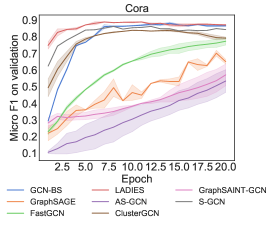
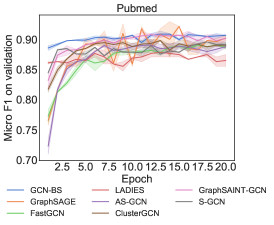
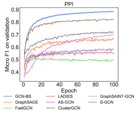
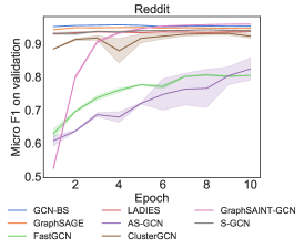
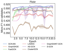
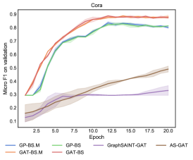
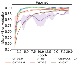
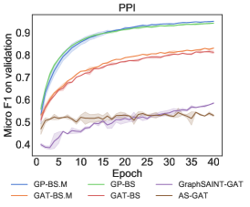
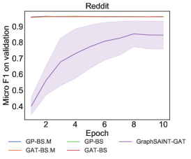
Figure 1: The convergence on validation in terms of epochs.

7.1 Results on Benchmark Data

We report the testing results on GCN and attentive GNN architectures in Table 2 and Table 3 respectively. We run the results of each algorithm $3$ times and report the mean and standard deviation. The results on the two layer GCN architecture show that our GCN-BS performs the best on most of datasets. The results on the two layer attentive GNN architecture show the superiority of our algorithms on training more complex GNN architectures. GraphSAINT or AS-GAT cannot compute the softmax of learned weights, but simply use the unnormalized weights to perform the aggregation. As a result, most of results from AS-GAT and GraphSAINT-GAT in Table 3 are worse than their results in Table 2. Thanks to the power of attentive structures in GNNs, our algorithms perform better results on PPI and Reddit compared with GCN-BS, and significantly outperform the results from AS-GAT and GraphSAINT-GAT.

7.2 Convergence

In this section, we analyze the convergences of comparison algorithms on the two layer GCN and attentive GNN architectures in Figure 1 in terms of epoch. We run all the algorithms $3$ times and show the mean and standard deviation. Our approaches consistently converge to better results with faster rates and lower variances in most of datasets like Pubmed, PPI, Reddit and Flickr compared with the state-of-the-art approaches. The GNN-BS algorithms perform very similar to GNN-BS.M, even though strictly speaking GNN-BS does not follow the rigorous MAB setting. Furthermore, we show a huge improvement on the training of attentive GNN architectures compared with GraphSAINT-GAT and AS-GAT. The convergences on validation in terms of timing (seconds), compared with layer sampling approaches, in Appendix C.1 show the similar results. We further give a discussion about timing among layer sampling approaches and graph sampling approaches in Appendix C.2.

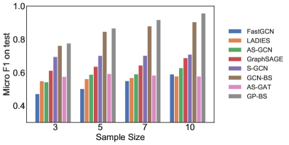
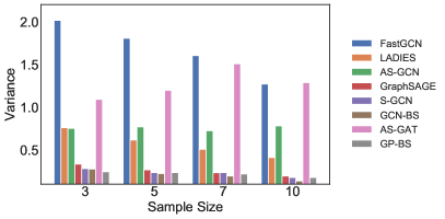
Figure 2: Comparisons on PPI by varying the sample sizes: (left) F1 score, (right) sample variances.

7.3 Sample Size Analysis

We analyze the sampling variances and accuracy as sample size varies using PPI data. Note that existing layer sampling approaches do not optimize the variances once the samplers are specified. As a result, their variances are simply fixed [25], while our approaches asymptotically appoach the optimum. For comparison, we train our models until convergence, then compute the average sampling variances. We show the results in Figure 2. The results are grouped into two categories, i.e. results for GCNs and attentive GNNs respectively. The sampling variances of our approaches are smaller in each group, and even be smaller than the variances of S-GCN that leverages a variance reduction solver. This explains the performances of our approaches on testing Micro F1 scores. We also find that the overall sampling variances of node-wise approaches are way better than those of layer-wise approaches.

8 Conclusions

In this paper, we show that the optimal layer samplers based on importance sampling for training general graph neural networks are computationally intractable, since it needs all the neighbors’ hidden embeddings or learned weights. Instead, we re-formulate the sampling problem as a bandit problem that requires only partial knowledges from neighbors being sampled. We propose two algorithms based on multi-armed bandit and MAB with multiple plays, and show the variance of our bandit sampler asymptotically approaches the optimum within a factor of $3$. Furthermore, our algorithms are not only applicable to GCNs but more general architectures like attentive GNNs. We empirically show that our algorithms can converge to better results with faster rates and lower variances compared with state-of-the-art approaches.

Appendix A Algorithms

Algorithm 2 $\mathrm{EXP3}(q_{i}^{t},w_{i}^{t},r_{i}^{t},S_{i}^{t})$.

1:$\eta=0.4$, sample size $k$, neighbor size $n=|\mathcal{N}_{i}|$, $\delta=\sqrt{(1-\eta)\eta^{4}k^{5}\ln(n/k)/(Tn^{4})}$.

2:Set

$$\hat{r}_{ij}(t)=r_{ij}(t)/q_{ij}(t)\;\text{if}\;j\in S_{i}^{t}\;\text{else}\;0$$

$$w_{ij}(t+1)=w_{ij}(t)\exp(\delta\,\hat{r}_{ij}(t)/n)$$

3:Set $q_{ij}(t+1)\leftarrow(1-\eta)\frac{w_{ij}(t+1)}{\sum_{j\in\mathcal{N}_{i}}w_{ij}(t+1)}+\frac{\eta}{n},\,\,\,\,\,\text{for}\,\,j\in\mathcal{N}_{i}$

Algorithm 3 EXP3.M$(q_{i}^{t},w_{i}^{t},r_{i}^{t},S_{i}^{t})$

1:$\eta=0.4$, sample size $k$, neighbor size $n=\left|\mathcal{N}_{i}\right|$, $\delta=\sqrt{(1-\eta)\eta^{4}k^{5}\ln(n/k)/(Tn^{4})}$, $U_{i}^{t}=\emptyset$.

2:For $j\in\mathcal{N}_{i}$ set

$$\hat{r}_{ij}(t)=\begin{cases}r_{ij}(t)/q_{ij}(t)&\text{if}\;j\in S_{i}^{t}\\ 0&\text{otherwise}\end{cases}$$

$$w_{ij}(t+1)=\begin{cases}w_{ij}(t)\exp(\delta\hat{r}_{ij}(t)/n)&\text{if}\;j\notin U_{i}^{t}\\ w_{ij}(t)&\text{otherwise}\end{cases}$$

3:if $\mathop{\max}_{j\in\mathcal{N}_{i}}w_{ij}(t+1)\geq(\frac{1}{k}-\frac{\eta}{n})\sum_{j\in\mathcal{N}_{i}}{w_{ij}(t+1)/(1-\eta)}$ then

4:     Decide $a_{t}$ so as to satisfy

$$\frac{a_{t}}{\sum_{w_{ij}(t+1)\geq a_{t}}a_{t}+\sum_{w_{ij}(t+1)<a_{t}}w_{ij}(t+1)}=(\frac{1}{k}-\frac{\eta}{n})/(1-\eta)$$

5:     Set $U_{i}^{t+1}=\{j:w_{ij}(t+1)\geq a_{t}\}$

6:else

7:     Set $U_{i}^{t+1}=\emptyset$

8:end if

9:Set $w_{ij}^{\prime}(t+1)=\begin{cases}w_{ij}(t+1)&\text{if}\;j\in\mathcal{N}_{i}\backslash U_{i}^{t+1}\\ a_{t}&\text{if}\;j\in U_{i}^{t}\end{cases}$

10:Set $q_{ij}(t+1)=k\left((1-\eta)\frac{w_{ij}^{\prime}(t+1)}{\sum_{j\in\mathcal{N}_{i}}w_{ij}^{\prime}(t+1)}+\frac{\eta}{n}\right)$ for $j\in\mathcal{N}_{i}$

Algorithm 4 DepRound$(k,(q_{1},q_{2},...,q_{K}))$

1:Input: Sample size $k(k<K)$, sample distribution $(q_{1},q_{2},...,q_{K})$ with $\sum_{i=1}^{K}q_{i}=k$

2:Output: Subset of $[K]$ with $k$ elements

3:while there is an $i$ with $0<q_{i}<1$ do

4:     Choose distinct $i$ and $j$ with $0<q_{i}<1$ and $0<q_{j}<1$

5:     Set $\beta=\min\{1-q_{i},q_{j}\}$ and $\gamma=\min\{q_{i},1-q_{j}\}$

6:     Update $q_{i}$ and $q_{j}$ as

$$(q_{i},q_{j})=\begin{cases}(q_{i}+\beta,q_{j}-\beta)\;\text{with probability}\;\frac{\gamma}{\beta+\gamma}\\ (q_{i}-\gamma,q_{j}+\gamma)\;\text{with probability}\;\frac{\beta}{\beta+\gamma}\end{cases}$$

7:end while

8:return $\{i:q_{i}=1,1\leq i\leq K\}$

Appendix B Proofs

Proposition 1.

$\hat{\mu}_{i}=\sum_{j_{s}\in S_{i}}\frac{\alpha_{ij_{s}}}{q_{ij_{s}}}h_{j_{s}}$ is the unbiased estimator of $\mu_{i}=\sum_{j\in\mathcal{N}_{i}}\alpha_{ij}h_{j}$ given that $S_{i}$ is sampled from $q_{i}$ using the DepRound sampler $Q_{i}$, where $S_{i}$ is the selected $k$-subset neighbors of vertex $i$.

Proof.

Let us denote $Q_{i,S_{i}}$ as the probability of vertex $v_{i}$ choosing any $k$-element subset $S_{i}\subset\mathcal{N}_{i}$ from the $K$-element set $\mathcal{N}_{i}$ using DepRound sampler $Q_{i}$. This sampler follows the alternative sampling distribution $q_{i}=(q_{ij_{1}},...,q_{ij_{K}})$ where $q_{ij_{s}}$ denotes the alternative probability of sampling neighbor $v_{j_{s}}$. This sampler is guaranteed to satisfy $\sum_{S_{i}:j\in S_{i}}Q_{i,S_{i}}=q_{ij}$, i.e. the sum over the probabilities of all subsets $S_{i}$ that contains element $j$ equals the probability $q_{ij}$.

$$\mathbb{E}\left[\hat{\mu}_{i}\right] =\mathbb{E}\left[\sum_{j_{s}\in S_{i}}\frac{\alpha_{ij_{s}}}{q_{ij_{s}}}h_{j_{s}}\right]$$ (12)

$$=\sum_{S_{i}\subset\mathcal{N}_{i}}Q_{i,S_{i}}\sum_{j_{s}\in S_{i}}\frac{\alpha_{ij_{s}}}{q_{ij_{s}}}h_{j_{s}}$$ (13)

$$=\sum_{j\in\mathcal{N}_{i}}\sum_{S_{i}:j\in S_{i}}Q_{i,S_{i}}\frac{\alpha_{ij}}{q_{ij}}h_{j}$$ (14)

$$=\sum_{j\in\mathcal{N}_{i}}\frac{\alpha_{ij}}{q_{ij}}h_{j}\sum_{S_{i}:j\in S_{i}}Q_{i,S_{i}}$$ (15)

$$=\sum_{j\in\mathcal{N}_{i}}\frac{\alpha_{ij}}{q_{ij}}h_{j}q_{ij}$$ (16)

$$=\sum_{j\in\mathcal{N}_{i}}\alpha_{ij}h_{j}$$ (17)

∎

Proposition 2.

The effective variance can be approximated by $\mathbb{V}_{e}(Q_{i})\leq\sum_{j_{s}\in\mathcal{N}_{i}}\frac{\alpha_{ij_{s}}}{q_{ij_{s}}}\|h_{j_{s}}\|^{2}$.

Proof.

The variance is

$$\mathbb{V}(Q_{i}) =\mathbb{E}\left[\left\|\sum_{j_{s}\in S_{i}}\frac{\alpha_{ij_{s}}}{q_{ij_{s}}}h_{j_{s}}-\sum_{j\in\mathcal{N}_{i}}\alpha_{ij}h_{j}\right\|^{2}\right]$$

$$=\sum_{S_{i}\subset\mathcal{N}_{i}}Q_{i,S_{i}}\left\|\sum_{j_{s}\in S_{i}}\frac{\alpha_{ij_{s}}}{q_{ij_{s}}}h_{j_{s}}\right\|^{2}-\left\|\sum_{j\in\mathcal{N}_{i}}\alpha_{ij}h_{j}\right\|^{2}.$$

Therefore the effective variance has following upper bound:

$$\mathbb{V}_{e}(Q_{i}) =\sum_{S_{i}\subset\mathcal{N}_{i}}Q_{i,S_{i}}\left\|\sum_{j_{s}\in S_{i}}\frac{\alpha_{ij_{s}}}{q_{ij_{s}}}h_{j_{s}}\right\|^{2}$$

$$\leq\sum_{S_{i}\subset\mathcal{N}_{i}}Q_{i,S_{i}}\sum_{j_{s}\in S_{i}}\alpha_{ij_{s}}\left\|\frac{h_{j_{s}}}{q_{ij_{s}}}\right\|^{2}\;(Jensen^{\prime}s\,Inequality)$$

$$=\sum_{j_{s}\in\mathcal{N}_{i}}\sum_{S_{i}:j_{s}\in S_{i}}Q_{i,S_{i}}\alpha_{ij_{s}}\left\|\frac{h_{j_{s}}}{q_{ij_{s}}}\right\|^{2}$$

$$=\sum_{j_{s}\in\mathcal{N}_{i}}\frac{\alpha_{ij_{s}}}{q_{ij_{s}}^{2}}\|h_{j_{s}}\|^{2}\sum_{S_{i}:j_{s}\in S_{i}}Q_{i,S_{i}}$$

$$=\sum_{j_{s}\in\mathcal{N}_{i}}\frac{\alpha_{ij_{s}}}{q_{ij_{s}}}\|h_{j_{s}}\|^{2}$$

∎

Proposition 3.

The negative derivative of the approximated effective variance $\sum_{j_{s}\in\mathcal{N}_{i}}\frac{\alpha_{ij_{s}}}{q_{ij_{s}}}\|h_{j_{s}}\|^{2}$ w.r.t $Q_{i,S_{i}}$, i.e. the reward of $v_{i}$ choosing $S_{i}$ at $t$, is $r_{i,S_{i}}(t)=\sum_{j_{s}\in S_{i}}\frac{\alpha_{ij_{s}}}{q_{ij_{s}}(t)^{2}}\|h_{j_{s}}(t)\|^{2}$.

Proof.

Define the upper bound as $\hat{\mathbb{V}}_{e}(Q_{i})=\sum_{j_{s}\in\mathcal{N}_{i}}\frac{\alpha_{ij_{s}}}{q_{ij_{s}}}\|h_{j_{s}}\|^{2}$, then its derivative is

$$\nabla_{Q_{i,S_{i}}}\hat{\mathbb{V}}_{e}(Q_{i}) =\nabla_{Q_{i,S_{i}}}\sum_{j_{s}\in\mathcal{N}_{i}}\frac{\alpha_{ij_{s}}}{q_{ij_{s}}}\|h_{j_{s}}\|^{2}$$

$$=\nabla_{Q_{i,S_{i}}}\sum_{j_{s}\in\mathcal{N}_{i}}\frac{\alpha_{ij_{s}}}{\sum_{S_{i}^{\prime}:j_{s}\in S_{i}^{\prime}}Q_{i,S_{i}^{\prime}}}\|h_{j_{s}}\|^{2}$$

$$=\nabla_{Q_{i,S_{i}}}\sum_{j_{s}\in S_{i}}\frac{\alpha_{ij_{s}}}{\sum_{S_{i}^{\prime}:j_{s}\in S_{i}^{\prime}}Q_{i,S_{i}^{\prime}}}\|h_{j_{s}}\|^{2}$$

$$=-\sum_{j_{s}\in S_{i}}\frac{\alpha_{j_{s}}}{q_{ij_{s}}^{2}}\|h_{j_{s}}\|^{2}\;(chain\,rule)$$

∎

Before we give the proof of Theorem 1, we first prove the following Lemma 1 that will be used later.

Lemma 1.

For any real value constant $\eta\leq 1$ and any valid distributions $Q_{i}^{t}$ and $Q_{i}^{\star}$ we have

$$(1-2\eta)\mathbb{V}_{e}^{t}(Q_{i}^{t})-(1-\eta)\mathbb{V}_{e}^{t}(Q_{i}^{\star})\leq\langle Q_{i}^{t}-Q_{i}^{\star},\nabla_{Q_{i}^{t}}\mathbb{V}_{e}^{t}(Q_{i}^{t})\rangle+\eta\langle Q_{i}^{\star},\nabla_{Q_{i}^{t}}\mathbb{V}_{e}^{t}(Q_{i}^{t})\rangle$$ (18)

Proof.

The function $\mathbb{V}_{e}^{t}(Q)$ is convex with respect to $Q$, hence for any $Q_{i}^{t}$ and $Q_{i}^{\star}$ we have

$$\mathbb{V}_{e}^{t}(Q_{i}^{t})-\mathbb{V}_{e}^{t}(Q_{i}^{\star})\leq\langle Q_{i}^{t}-Q_{i}^{\star},\nabla_{Q_{i}^{t}}\mathbb{V}_{e}^{t}(Q_{i}^{t})\rangle.$$ (19)

Multiplying both sides of this inequality by $1-\eta$, we have

$$(1-\eta)\mathbb{V}_{e}^{t}(Q_{i}^{t})-(1-\eta)\mathbb{V}_{e}^{t}(Q_{i}^{\star})$$ (20)

$$\leq\langle Q_{i}^{t}-Q_{i}^{\star},\nabla_{Q_{i}^{t}}\mathbb{V}_{e}^{t}(Q_{i}^{t})\rangle-\eta\langle Q_{i}^{t}-Q_{i}^{\star},\nabla_{Q_{i}^{t}}\mathbb{V}_{e}^{t}(Q_{i}^{t})\rangle.$$ (21)

In the following, we prove this Lemma in our two bandit settings: adversary MAB setting and adversary MAB with multiple plays setting.

In adversary MAB setting, we have

$$\langle Q_{i}^{t},\nabla_{Q_{i}^{t}}\mathbb{V}_{e}^{t}(Q_{i}^{t})\rangle =-\sum_{j\in\mathcal{N}_{i}}q_{ij}(t)\frac{\alpha_{ij}^{2}}{k\cdot q_{ij}(t)^{2}}\|h_{j}(t)\|^{2}$$ (22)

$$=-\mathbb{V}_{e}^{t}(Q_{i}^{t})$$ (23)

In adversary MAB with multiple plays setting, we use the approximated effective variance $\sum_{j_{s}\in\mathcal{N}_{i}}\frac{\alpha_{ij_{s}}}{q_{ij_{s}}}\|h_{j_{s}}\|^{2}$ derived in Proposition 2. For notational simplicity, we denote the approximated effective variance as $\mathbb{V}_{e}$ in the following. We have

$$\langle Q_{i}^{t},\nabla_{Q_{i}^{t}}\mathbb{V}_{e}^{t}(Q_{i}^{t})\rangle =-\sum_{S_{i}\subset\mathcal{N}_{i}}Q_{i,S_{i}}^{t}\sum_{j_{s}\in S_{i}}\frac{\alpha_{ij_{s}}}{q_{ij_{s}}(t)^{2}}\|h_{j_{s}}\|^{2}$$ (24)

$$=-\sum_{j_{s}\in\mathcal{N}_{i}}\frac{\alpha_{ij_{s}}}{q_{ij_{s}}(t)^{2}}\|h_{j_{s}}\|^{2}\sum_{S_{i}:j_{s}\in S_{i}}Q_{i,S_{i}}^{t}$$ (25)

$$=-\sum_{j_{s}\in\mathcal{N}_{i}}\frac{\alpha_{ij_{s}}}{q_{ij_{s}}(t)}\|h_{j_{s}}\|^{2}$$ (26)

$$=-\mathbb{V}_{e}^{t}(Q_{i}^{t}).$$ (27)

The equation (24) holds because of Proposition 3.

At last, we conclude the proof

$$(1-\eta)\mathbb{V}_{e}^{t}(Q_{i}^{t})-(1-\eta)\mathbb{V}_{e}^{t}(Q_{i}^{\star})$$ (28)

$$\leq\langle Q_{i}^{t}-Q_{i}^{\star},\nabla_{Q_{i}^{t}}\mathbb{V}_{e}^{t}(Q_{i}^{t})\rangle-\eta\langle Q_{i}^{t}-Q_{i}^{\star},\nabla_{Q_{i}^{t}}\mathbb{V}_{e}^{t}(Q_{i}^{t})\rangle$$ (29)

$$=\langle Q_{i}^{t}-Q_{i}^{\star},\nabla_{Q_{i}^{t}}\mathbb{V}_{e}^{t}(Q_{i}^{t})\rangle+\eta\langle Q_{i}^{\star},\nabla_{Q_{i}^{t}}\mathbb{V}_{e}^{t}(Q_{i}^{t})\rangle+\eta\mathbb{V}_{e}^{t}(Q_{i}^{t}).$$ (30)

∎

Theorem 1.

Using Algorithm 1 with $\eta=0.4$ and $\delta=\sqrt{(1-\eta)\eta^{4}k^{5}\ln(n/k)/(Tn^{4})}$ to minimize effective variance with respect to $\{Q_{i}^{t}\}_{1\leq t\leq T}$, we have

$$\sum_{t=1}^{T}\mathbb{V}_{e}^{t}(Q_{i}^{t})\leq 3\sum_{t=1}^{T}\mathbb{V}_{e}^{t}(Q_{i}^{\star})+10\sqrt{\frac{Tn^{4}\ln(n/k)}{k^{3}}}$$ (31)

where $T\geq\ln(n/k)n^{2}(1-\eta)/(k\eta^{2})$ and $n=\left|\mathcal{N}_{i}\right|$.

Proof.

First we explain why condition $T\geq\ln(n/k)n^{2}(1-\eta)/(k\eta^{2})$ ensures that $\delta\hat{r}_{ij}(t)\leq 1$,

$$\delta\hat{r}_{ij}(t) =\sqrt{\frac{(1-\eta)\eta^{4}k^{5}\ln(n/k)}{Tn^{4}}}\cdot\frac{\alpha_{ij}(t)}{q_{ij}^{3}(t)}\|h_{j}(t)\|^{2}$$ (32)

$$\leq\sqrt{\frac{(1-\eta)\eta^{4}k^{5}\ln(n/k)}{Tn^{4}}}\cdot\frac{n^{3}}{k^{3}\eta^{3}}$$ (33)

$$\leq 1$$ (34)

Assuming $\|h_{j}(t)\|\leq 1$, inequality (33) holds because $\alpha_{ij}(t)\leq 1$ and $q_{ij}(t)\geq k\eta/n$. Then replace $T$ by the condition, we get $\delta\hat{r}_{ij}(t)\leq 1$.

Let $W_{i}(t)$, $W_{i}^{\prime}(t)$ denote $\sum_{j\in\mathcal{N}_{i}}w_{ij}(t)$, $\sum_{j\in\mathcal{N}_{i}}w_{ij}^{\prime}(t)$ respectively. Then for any $t=1,2,...,T$,

$$\frac{W_{i}(t+1)}{W_{i}(t)} =\sum_{j\in\mathcal{N}_{i}\backslash U_{i}^{t}}\frac{w_{ij}(t+1)}{W_{i}(t)}+\sum_{j\in U_{i}^{t}}\frac{w_{ij}(t+1)}{W_{i}(t)}$$ (35)

$$=\sum_{j\in\mathcal{N}_{i}\backslash U_{i}^{t}}\frac{w_{ij}(t)}{W_{i}(t)}\cdot\exp(\delta\hat{r}_{ij}(t))+\sum_{j\in U_{i}^{t}}\frac{w_{ij}(t)}{W_{i}(t)}$$ (36)

$$\leq\sum_{j\in\mathcal{N}_{i}\backslash U_{i}^{t}}\frac{w_{ij}(t)}{W_{i}(t)}\left[1+\delta\hat{r}_{ij}(t)+\left(\delta\hat{r}_{ij}(t)\right)^{2}\right]+\sum_{j\in U_{i}^{t}}\frac{w_{ij}(t)}{W_{i}(t)}$$ (37)

$$=1+\frac{W_{i}^{\prime}(t)}{W_{i}(t)}\sum_{j\in\mathcal{N}_{i}\backslash U_{i}^{t}}\frac{w_{ij}(t)}{W_{i}^{\prime}(t)}\left[\delta\hat{r}_{ij}(t)+\left(\delta\hat{r}_{ij}(t)\right)^{2}\right]$$ (38)

$$=1+\frac{W_{i}^{\prime}(t)}{W_{i}(t)}\sum_{j\in\mathcal{N}_{i}\backslash U_{i}^{t}}\frac{q_{ij}(t)/k-\eta/n}{1-\eta}\left[\delta\hat{r}_{ij}(t)+\left(\delta\hat{r}_{ij}(t)\right)^{2}\right]$$ (39)

$$\leq 1+\frac{\delta}{k(1-\eta)}\sum_{j\in\mathcal{N}_{i}\backslash U_{i}^{t}}q_{ij}(t)\hat{r}_{ij}(t)+\frac{\delta^{2}}{k(1-\eta)}\sum_{j\in\mathcal{N}_{i}\backslash U_{i}^{t}}q_{ij}(t)\hat{r}_{ij}^{2}(t)$$ (40)

Inequality (37) uses $e^{a}\leq 1+a+a^{2}$ for $a\leq 1$. Equality (39) holds because of update equation of $q_{ij}(t)$ defined in EXP3.M. Inequality (40) holds because $\frac{W_{i}^{\prime}(t)}{W_{i}(t)}\leq 1$. Since $1+x\leq e^{x}$ for $x\geq 0$, we have

$$\ln\frac{W_{i}(t+1)}{W_{i}(t)}\leq\frac{\delta}{k(1-\eta)}\sum_{j\in\mathcal{N}_{i}\backslash U_{i}^{t}}q_{ij}(t)\hat{r}_{ij}(t)+\frac{\delta^{2}}{k(1-\eta)}\sum_{j\in\mathcal{N}_{i}\backslash U_{i}^{t}}q_{ij}(t)\hat{r}_{ij}^{2}(t)$$ (41)

If we sum, for $1\leq t\leq T$, we get the following telescopic sum

$$\ln\frac{W_{i}(T+1)}{W_{i}(1)} =\sum_{t=1}^{T}\ln\frac{W_{i}(t+1)}{W_{i}(t)}$$ (42)

$$\leq\frac{\delta}{k(1-\eta)}\sum_{t=1}^{T}\sum_{j\in\mathcal{N}_{i}\backslash U_{i}^{t}}q_{ij}(t)\hat{r}_{ij}(t)+\frac{\delta^{2}}{k(1-\eta)}\sum_{t=1}^{T}\sum_{j\in\mathcal{N}_{i}\backslash U_{i}^{t}}q_{ij}(t)\hat{r}_{ij}^{2}(t)$$ (43)

$$\leq\frac{\delta}{k(1-\eta)}\sum_{t=1}^{T}\sum_{j\in\mathcal{N}_{i}\backslash U_{i}^{t}}q_{ij}(t)\hat{r}_{ij}(t)+\frac{\delta^{2}}{k(1-\eta)}\sum_{t=1}^{T}\sum_{j\in\mathcal{N}_{i}}q_{ij}(t)\hat{r}_{ij}^{2}(t)$$ (44)

On the other hand, for any subset $S$ containing k elements,

$$\ln\frac{W_{i}(T+1)}{W_{i}(1)} \geq\ln\frac{\sum_{j\in S}w_{ij}(T+1)}{W_{i}(1)}$$ (45)

$$\geq\frac{\sum_{j\in S}\ln w_{ij}(T+1)}{k}-\ln\frac{n}{k}$$ (46)

$$\geq\frac{\delta}{k}\sum_{j\in S}\sum_{t:j\notin U_{i}^{t}}\hat{r}_{ij}(t)-\ln\frac{n}{k}$$ (47)

The inequality (46) uses the fact that

$$\sum_{j\in S}w_{ij}(T+1)\geq k(\prod_{j\in S}w_{ij}(T+1))^{1/k}$$

The equation (47) uses the fact that

$$w_{ij}(T+1)=\exp(\delta\sum_{t:j\notin U_{i}^{t}}\hat{r}_{ij}(t))$$

From (44) and  (47), we get

$$\frac{\delta}{k}\sum_{j\in S}\sum_{t:j\notin U_{i}^{t}}\hat{r}_{ij}(t)-\ln\frac{n}{k}\leq\frac{\delta}{k(1-\eta)}\sum_{t=1}^{T}\sum_{j\in\mathcal{N}_{i}\backslash U_{i}^{t}}q_{ij}(t)\hat{r}_{ij}(t)+\frac{\delta^{2}}{k(1-\eta)}\sum_{t=1}^{T}\sum_{j\in\mathcal{N}_{i}\backslash U_{i}^{t}}q_{ij}(t)\hat{r}_{ij}^{2}(t)$$ (48)

And we have the following inequality

$$\frac{\delta}{k}\sum_{j\in S}\sum_{t:j\in U_{i}^{t}}r_{ij}(t) =\frac{\delta}{k}\sum_{j\in S}\sum_{t:j\in U_{i}^{t}}q_{ij}(t)\hat{r}_{ij}(t)$$ (49)

$$\leq\frac{\delta}{k(1-\eta)}\sum_{t=1}^{T}\sum_{j\in U_{i}^{t}}q_{ij}(t)\hat{r}_{ij}(t)$$ (50)

The equality (49) holds beacuse $r_{ij}(t)=q_{ij}\hat{r}_{ij}(t)$ when $j\in S_{i}^{t}$ and $U_{i}^{t}\subseteq S_{i}^{t}$ bacause $q_{ij}^{t}=1$ for all $j\in U_{i}^{t}$.

Then add inequality (50) in  (48) we have

$$\frac{\delta}{k}\sum_{j\in S}\sum_{t:j\in U_{i}^{t}}r_{ij}(t)+\frac{\delta}{k}\sum_{j\in S}\sum_{t:j\notin U_{i}^{t}}\hat{r}_{ij}(t)-\ln\frac{n}{k}$$ (51)

$$\leq\frac{\delta}{k(1-\eta)}\sum_{t=1}^{T}\sum_{j\in\mathcal{N}_{i}}q_{ij}(t)\hat{r}_{ij}(t)+\frac{\delta^{2}}{k(1-\eta)}\sum_{t=1}^{T}\sum_{j\in\mathcal{N}_{i}}q_{ij}(t)\hat{r}_{ij}^{2}(t)$$ (52)

Given $q_{ij}(t)$ we have $\mathbb{E}[\hat{r}_{ij}^{2}(t)]=r_{ij}^{2}(t)/q_{ij}(t)$, hence, taking expectation of (51) yields that

$$\frac{\delta}{k}\sum_{t=1}^{T}\sum_{j\in S}r_{ij}(t)-\ln\frac{n}{k}\leq\frac{\delta}{k(1-\eta)}\sum_{t=1}^{T}\sum_{j\in\mathcal{N}_{i}}q_{ij}(t)r_{ij}(t)+\frac{\delta^{2}}{k(1-\eta)}\sum_{t=1}^{T}\sum_{j\in\mathcal{N}_{i}}r_{ij}^{2}(t)$$ (53)

By multiplying (53) by $Q_{i,S}^{\star}$ and summing over $S$, we get

$$\frac{\delta}{k}\sum_{t=1}^{T}\sum_{S\subset\mathcal{N}_{i}}Q_{i,S}^{\star}\sum_{j\in S}r_{ij}(t)-\ln\frac{n}{k}\leq\frac{\delta}{k(1-\eta)}\sum_{t=1}^{T}\sum_{j\in\mathcal{N}_{i}}q_{ij}(t)r_{ij}(t)+\frac{\delta^{2}}{k(1-\eta)}\sum_{t=1}^{T}\sum_{j\in\mathcal{N}_{i}}r_{ij}^{2}(t)$$ (54)

As

$$\sum_{j\in\mathcal{N}_{i}}q_{ij}(t)r_{ij}(t) =\sum_{j\in\mathcal{N}_{i}}\sum_{S_{i}:j\in S_{i}}Q_{i,S_{i}}^{t}r_{ij}(t)$$ (55)

$$=\sum_{S_{i}\subset\mathcal{N}_{i}}Q_{i,S_{i}}^{t}\sum_{j\in S_{i}}r_{ij}(t)$$ (56)

$$=-\sum_{S_{i}\subset\mathcal{N}_{i}}Q_{i,S_{i}}^{t}\nabla_{Q_{i,S_{i}}^{t}}\mathbb{V}_{e}^{t}(Q_{i,S_{i}}^{t})$$ (57)

$$=-\langle Q_{i}^{t},\nabla_{Q_{i}^{t}}\mathbb{V}_{e}^{t}(Q_{i}^{t})\rangle$$ (58)

By plugging (58) in (54) and rearranging it, we find

$$\sum_{t=1}^{T}\langle Q_{i}^{t}-Q_{i}^{\star},\nabla_{Q_{i}^{t}}\mathbb{V}_{e}^{t}(Q_{i}^{t})\rangle+\eta\sum_{t=1}^{T}\langle Q_{i}^{\star},\nabla_{Q_{i}^{t}}\mathbb{V}_{e}^{t}(Q_{i}^{t})\rangle$$ (59)

$$\leq\delta\sum_{t=1}^{T}\sum_{j\in\mathcal{N}_{i}}r_{ij}^{2}(t)+\frac{(1-\eta)k}{\delta}\ln(n/k)$$

Using Lemma 1, we have

$$(1-2\eta)\sum_{t=1}^{T}\mathbb{V}_{e}^{t}(Q_{i}^{t})-(1-\eta)\sum_{t=1}^{T}\mathbb{V}_{e}^{t}(Q_{i}^{\star})\leq\delta\sum_{t=1}^{T}\sum_{j\in\mathcal{N}_{i}}r_{ij}^{2}(t)+\frac{(1-\eta)k}{\delta}\ln(n/k)$$ (60)

Finally, we know that

$$\sum_{j\in\mathcal{N}_{i}}r_{ij}^{2}(t) =\sum_{j\in\mathcal{N}_{i}}\frac{\alpha_{ij}(t)^{2}}{q_{ij}(t)^{4}}$$ (61)

$$\leq\sum_{j\in\mathcal{N}_{i}}\alpha_{ij}(t)\frac{n^{4}}{k^{4}\eta^{4}}\;(because\,q_{ij}(t)\geq k\eta/n)$$ (62)

$$=\frac{n^{4}}{k^{4}\eta^{4}}$$ (63)

By setting $\eta=0.4$ and $\delta=\sqrt{(1-\eta)\eta^{4}k^{5}\ln(n/k)/(Tn^{4})}$, we get the upper bound.

∎

Appendix C Experiments

C.1 Convergences

We show the convergences on validation in terms of timing (seconds) in Figure 3 and Figure 4. Basically, our algorithms converge to much better results in nearly same duration compared with other “layer sampling” approaches.

Note that we cannot complete the training of AS-GAT on Reddit because of memory issues.

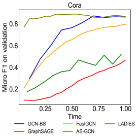
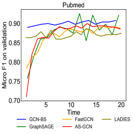
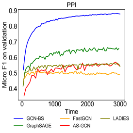
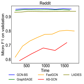
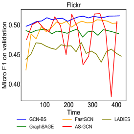
Figure 3: The convergence in timing (seconds) on GCNs.

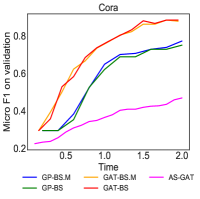
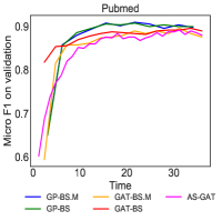
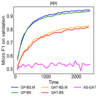
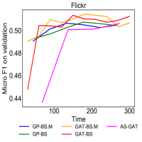
Figure 4: The convergence in timing (seconds) on attentive GNNs.

C.2 Discussions on Timings between Layer Sampling and Graph Sampling Paradigms

Note that the comparisons of timing between “graph sampling” and “layer sampling” paradigms have been studied recently in [7, 24]. As a result, we do not compare the timing with “graph sampling” approaches. Under certain conditions, the graph sampling approaches should be faster than layer sampling approaches. That is, graph sampling approaches are designed for graph data that all vertices have labels. Under such condition, the floating point operations analyzed in [7] are maximally utilized compared with the “layer sampling” paradigm. However, in practice, there are large amount of graph data with labels only on some types of vertices, such as the graphs in [16]. “Graph sampling” approaches are not applicable to cases where only partial vertices have labels. To summarize, the “layer sampling” approaches are more flexible and general compared with “graph sampling” approaches in many cases.

C.3 Results on OGB

We report our results on OGB protein dataset [13]. We set the learning rate as 1e-3, batch size as 256, the dimension of hidden embeddings as 64, sample size as 10 and epochs as 200. We save the model based on the best results on validation and report results on testing data. We run the experiment 10 times with different random seeds to compute the average and standard deviation of the results. Our result of GP-BS on protein dataset performs the best until we submitted this paper. Please find our implementations at https://github.com/xavierzw/ogb-geniepath-bs.

Dateset	Mean	Std	#experiments
ogbn-proteins	$0.78253$	$0.00352$	$10$

References

- Auer et al. [2002] P. Auer, N. Cesa-Bianchi, Y. Freund, and R. E. Schapire. The nonstochastic multiarmed bandit problem. SIAM journal on computing, 32(1):48–77, 2002.
- Ba et al. [2016] J. L. Ba, J. R. Kiros, and G. E. Hinton. Layer normalization. arXiv preprint arXiv:1607.06450, 2016.
- Battaglia et al. [2018] P. W. Battaglia, J. B. Hamrick, V. Bapst, A. Sanchez-Gonzalez, V. Zambaldi, M. Malinowski, A. Tacchetti, D. Raposo, A. Santoro, R. Faulkner, et al. Relational inductive biases, deep learning, and graph networks. arXiv preprint arXiv:1806.01261, 2018.
- Burtini et al. [2015] G. Burtini, J. Loeppky, and R. Lawrence. A survey of online experiment design with the stochastic multi-armed bandit. arXiv preprint arXiv:1510.00757, 2015.
- Chen et al. [2017] J. Chen, J. Zhu, and L. Song. Stochastic training of graph convolutional networks with variance reduction. arXiv preprint arXiv:1710.10568, 2017.
- Chen et al. [2018] J. Chen, T. Ma, and C. Xiao. Fastgcn: fast learning with graph convolutional networks via importance sampling. arXiv preprint arXiv:1801.10247, 2018.
- Chiang et al. [2019] W.-L. Chiang, X. Liu, S. Si, Y. Li, S. Bengio, and C.-J. Hsieh. Cluster-gcn: An efficient algorithm for training deep and large graph convolutional networks. In Proceedings of the 25th ACM SIGKDD International Conference on Knowledge Discovery & Data Mining, pages 257–266, 2019.
- Dai et al. [2016] H. Dai, B. Dai, and L. Song. Discriminative embeddings of latent variable models for structured data. In International conference on machine learning, pages 2702–2711, 2016.
- Fout et al. [2017] A. Fout, J. Byrd, B. Shariat, and A. Ben-Hur. Protein interface prediction using graph convolutional networks. In Advances in Neural Information Processing Systems, pages 6530–6539, 2017.
- Gandhi et al. [2006] R. Gandhi, S. Khuller, S. Parthasarathy, and A. Srinivasan. Dependent rounding and its applications to approximation algorithms. Journal of the ACM (JACM), 53(3):324–360, 2006.
- Hamilton et al. [2017] W. Hamilton, Z. Ying, and J. Leskovec. Inductive representation learning on large graphs. In Advances in Neural Information Processing Systems, pages 1024–1034, 2017.
- Hu et al. [2019] B. Hu, Z. Zhang, C. Shi, J. Zhou, X. Li, and Y. Qi. Cash-out user detection based on attributed heterogeneous information network with a hierarchical attention mechanism. In Proceedings of the AAAI Conference on Artificial Intelligence, volume 33, pages 946–953, 2019.
- Hu et al. [2020] W. Hu, M. Fey, M. Zitnik, Y. Dong, H. Ren, B. Liu, M. Catasta, and J. Leskovec. Open graph benchmark: Datasets for machine learning on graphs. arXiv preprint arXiv:2005.00687, 2020.
- Huang et al. [2018] W. Huang, T. Zhang, Y. Rong, and J. Huang. Adaptive sampling towards fast graph representation learning. In Advances in Neural Information Processing Systems, pages 4558–4567, 2018.
- Kipf and Welling [2016] T. N. Kipf and M. Welling. Semi-supervised classification with graph convolutional networks. arXiv preprint arXiv:1609.02907, 2016.
- Liu et al. [2018] Z. Liu, C. Chen, X. Yang, J. Zhou, X. Li, and L. Song. Heterogeneous graph neural networks for malicious account detection. In Proceedings of the 27th ACM International Conference on Information and Knowledge Management, pages 2077–2085. ACM, 2018.
- Liu et al. [2019] Z. Liu, C. Chen, L. Li, J. Zhou, X. Li, L. Song, and Y. Qi. Geniepath: Graph neural networks with adaptive receptive paths. In Proceedings of the AAAI Conference on Artificial Intelligence, volume 33, pages 4424–4431, 2019.
- Salehi et al. [2017] F. Salehi, L. E. Celis, and P. Thiran. Stochastic optimization with bandit sampling. arXiv preprint arXiv:1708.02544, 2017.
- Schlichtkrull et al. [2018] M. Schlichtkrull, T. N. Kipf, P. Bloem, R. Van Den Berg, I. Titov, and M. Welling. Modeling relational data with graph convolutional networks. In European Semantic Web Conference, pages 593–607. Springer, 2018.
- Sen et al. [2008] P. Sen, G. Namata, M. Bilgic, L. Getoor, B. Galligher, and T. Eliassi-Rad. Collective classification in network data. AI magazine, 29(3):93–93, 2008.
- Uchiya et al. [2010] T. Uchiya, A. Nakamura, and M. Kudo. Algorithms for adversarial bandit problems with multiple plays. In International Conference on Algorithmic Learning Theory, pages 375–389. Springer, 2010.
- Veličković et al. [2017] P. Veličković, G. Cucurull, A. Casanova, A. Romero, P. Lio, and Y. Bengio. Graph attention networks. arXiv preprint arXiv:1710.10903, 2017.
- Wu et al. [2019] Z. Wu, S. Pan, F. Chen, G. Long, C. Zhang, and P. S. Yu. A comprehensive survey on graph neural networks. arXiv preprint arXiv:1901.00596, 2019.
- Zeng et al. [2019] H. Zeng, H. Zhou, A. Srivastava, R. Kannan, and V. Prasanna. Graphsaint: Graph sampling based inductive learning method. arXiv preprint arXiv:1907.04931, 2019.
- Zou et al. [2019] D. Zou, Z. Hu, Y. Wang, S. Jiang, Y. Sun, and Q. Gu. Layer-dependent importance sampling for training deep and large graph convolutional networks. In Advances in Neural Information Processing Systems, pages 11247–11256, 2019.