Abstract

Distribution regression refers to the supervised learning problem where labels are only available for groups of inputs instead of individual inputs. In this paper, we develop a rigorous mathematical framework for distribution regression where inputs are complex data streams. Leveraging properties of the expected signature and a recent signature kernel trick for sequential data from stochastic analysis, we introduce two new learning techniques, one feature-based and the other kernel-based. Each is suited to a different data regime in terms of the number of data streams and the dimensionality of the individual streams. We provide theoretical results on the universality of both approaches and demonstrate empirically their robustness to irregularly sampled multivariate time-series, achieving state-of-the-art performance on both synthetic and real-world examples from thermodynamics, mathematical finance and agricultural science.

1 INTRODUCTION

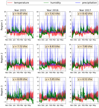
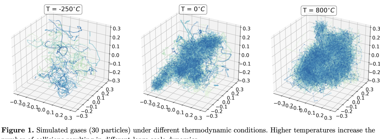
Distribution regression (dr) on sequential data describes the task of learning a function from a group of data streams to a single scalar target. For instance, in thermodynamics (Figure 1) one may be interested in determining the temperature of a gas from the set of trajectories described by its particles (Hill,, 1986; Reichl,, 1999; Schrödinger,, 1989). Similarly in quantitative finance practitioners may wish to estimate mean-reversion parameters from observed market dynamics (Papavasiliou et al.,, 2011; Gatheral et al.,, 2018; Balvers et al.,, 2000). Another example arises in agricultural science where the challenge consists in predicting the overall end-of-year crop yield from high-resolution climatic data across a field (Panda et al.,, 2010; Dahikar and Rode,, 2014; You et al.,, 2017).

dr techniques have been successfully applied to handle situations where the inputs in each group are vectors in $\mathbb{R}^{d}$. Recently, there has been an increased interest in extending these techniques to non-standard inputs such as images (Law et al.,, 2017) or persistence diagrams (Kusano et al.,, 2016). However dr for sequential data, such as multivariate time-series, has been largely ignored. The main challenges in this direction are the non-exchangeability of the points in a sequence, which naturally come with an order, and the fact that in many real world secenarios the points in a sequence are irregularly distributed across time.

Figure 1: Simulation of the trajectories traced by $20$ particles of an ideal gas in a $3$-d box under different thermodynamic conditions. Higher temperatures equate to a higher internal energy in the system which increases the number of collisions resulting in different large-scale dynamics of the gas.

In this paper we propose a framework for dr that addresses precisely the setting where the inputs within each group are complex data streams, mathematically thought of as Lipschitz continuous paths (Section 2). We formulate two distinct approaches, one feature-based and the other kernel-based, both relying on a recent tool from stochastic analysis known as the expected signature (Chevyrev and Oberhauser,, 2018; Chevyrev et al.,, 2016; Lyons et al.,, 2015; Ni,, 2012). Firstly, we construct a new set of features that are universal in the sense that any continuous function on distributions on paths can be uniformly well-approximated by a linear combination of these features (Section 3.1). Secondly, we introduce a universal kernel on distributions on paths given by the composition of the expected signature and a Gaussian kernel (Section 3.2), which can be evaluated with a kernel trick. The former method is more suitable to datasets containing a large number of low dimensional streams, whilst the latter is better for datasets with a low number of high dimensional streams. We demonstrate the versatility of our methods to handle interacting trajectories like the ones in Figure 1. We show how these two methods can used to provide practical dr algorithms for time-series, which are robust to irregular sampling and achieve state-of-the-art performance on synthetic and real-world dr examples (Section 5).

1.1 Problem definition

Consider $M$ input-output pairs $\{(\{\mathbf{x}^{i,p}\}_{p=1}^{N_{i}},y^{i})\}_{i=1}^{M}$, where each pair is given by a scalar target $y^{i}\in\mathbb{R}$ and a group of $N_{i}$ $d$-dimensional time-series of the form

$$\mathbf{x}^{i,p}=\{(t_{1},\mathbf{x}^{i,p}_{1}),\ldots,(t_{\ell_{i,p}},\mathbf{x}^{i,p}_{{\ell_{i,p}}})\},$$ (1)

of possibly unequal lengths $\ell_{i,p}\in\mathbb{N}$, with time-stamps $t_{1}$ $\leq$ $\ldots$ $\leq$ $t_{\ell_{i,p}}$ and values $\mathbf{x}^{i,p}_{k}\in\mathbb{R}^{d}$. Every d-dimensional time-series $\mathbf{x}^{i,p}$ can be naturally embedded into a Lipschitz-continuous path

$$x^{i,p}:[t_{1},t_{l_{i,p}}]\to\mathbb{R}^{d},$$ (2)

by piecewise linear interpolation with knots at $t_{1},\ldots,t_{l_{i,p}}$ such that $x^{i,p}_{t_{k}}=\mathbf{x}^{i,p}_{k}$. After having formally introduced a set of probability measures on this class of paths, we will summarize the information on each set $\{x^{i,p}\}_{p=1}^{N_{i}}$ by the empirical measure $\delta^{i}=\frac{1}{N_{i}}\sum_{p=1}^{N_{i}}\delta_{x^{i,p}}$ where $\delta_{x^{i,p}}$ is the Dirac measure centred at the path $x^{i,p}$. The supervised learning problem we propose to solve consists in learning an unknown function $F:\delta^{i}\mapsto y^{i}$.

2 THEORETICAL BACKGROUND

We begin by formally introducing the class of paths and the set of probability measures we are considering.

2.1 Paths and probability measures on paths

Let $0$ $\leq$ $a$ $<$ $T$ and $I=[a,T]$ be a closed time interval. Let $E$ be a Banach space of dimension $d\in\mathbb{N}$ (possibly infinite) with norm $\left\lVert\cdot\right\rVert_{E}$. For applications we will take $E:=\mathbb{R}^{d}$. We denote by $\mathcal{C}(I,E)$ the Banach space (Friz and Victoir,, 2010) of Lipschitz-continuous functions $x:I\to E$ equipped with the norm

$$\left\lVert x\right\rVert_{Lip}=\left\lVert x_{a}\right\rVert+\sup_{s,t\in I}\frac{\left\lVert x_{t}-x_{s}\right\rVert}{|t-s|}.$$ (3)

We will refer to any element $x\in\mathcal{C}(I,E)$ as an $E$-valued path. Given a compact subset of paths $\mathcal{X}\subset\mathcal{C}(I,E)$, we denote by $\mathcal{P}(\mathcal{X})$ the set of (Borel) probability measures on $\mathcal{X}$.

The signature has been shown to be an ideal feature map for paths (Lyons,, 2014). Analogously, the expected signature is an appropriate feature map for probability measures on paths. Both feature maps take values in the same feature space. In the next section we introduce the necessary mathematical background to describe the structure of this space.

2.2 A canonical Hilbert space of tensors $\mathcal{T}(E)$

In what follows $\oplus$ and $\otimes$ will denote the direct sum and the tensor product of vector spaces respectively. For example, $(\mathbb{R}^{d})^{\otimes 2}=\mathbb{R}^{d}\otimes\mathbb{R}^{d}$ is the space of $d\times d$ matrices and $(\mathbb{R}^{d})^{\otimes 3}$ is the space of $d\times d\times d$ tensors. By convention $E^{\otimes 0}=\mathbb{R}$. The following vector space will play a central role in this paper

$$\mathcal{T}(E)=\bigoplus_{k=0}^{\infty}E^{\otimes k}=\mathbb{R}\oplus E\oplus E^{\otimes 2}\oplus\ldots$$ (4)

If $\{e_{1},\ldots,e_{d}\}$ is a basis of $E$, the elements $\{e_{i_{1}}\otimes\ldots\otimes e_{i_{k}}\}_{(i_{1},\ldots,i_{k})\in\{1,\ldots,d\}^{k}}$ form a basis of $E^{\otimes k}$. For any $A\in\mathcal{T}(E)$ we denote by $A_{k}\in E^{\otimes k}$ the $k$-tensor component of $A$ and by $A^{(i_{1},\ldots,i_{k})}\in\mathbb{R}$ its $(i_{1}\ldots i_{k})^{th}$ coefficient. If $E$ is a Hilbert space with inner product $\langle\cdot,\cdot\rangle_{E}$, then there exists a canonical inner product $\langle\cdot,\cdot\rangle_{E^{\otimes k}}$ on each $E^{\otimes k}$ which extends by linearity to an inner product

$$\langle A,B\rangle_{\mathcal{T}(E)}=\sum_{k\geq 0}\langle A_{k},B_{k}\rangle_{E^{\otimes k}}$$ (5)

on $\mathcal{T}(E)$ that thus becomes also a Hilbert space (Chevyrev and Oberhauser,, 2018, Sec. 3).

2.3 The Signature of a path

The signature (Chen,, 1957; Lyons,, 1998, 2014) turns the complex structure of a path $x$ into a simpler vectorial representation given by an infinite sequence of iterated integrals. In this paper, the iterated integrals are defined in the classical Riemann-Stieltjes sense.

Definition 2.1.

The signature $S:\mathcal{C}(I,E)\to\mathcal{T}(E)$ is the map defined elementwise in the following way: the $0^{th}$ coefficient is always $S(x)^{(0)}=1$, whilst all the others are defined as

$$S(x)^{(i_{1}\ldots i_{k})}=\underset{a<u_{1}<\ldots<u_{k}<T}{\int\ldots\int}dx^{(i_{1})}_{u_{1}}\ldots dx^{(i_{k})}_{u_{k}}\in\mathbb{R},$$ (6)

where $t\mapsto x^{(i)}_{t}$ denotes the $i^{th}$ path-coordinate of $x$.

It is well known that any continuous function on a compact subset of $\mathbb{R}^{d}$ can be uniformly well approximated by polynomials (Conway,, 2019, Thm. 8.1). In full analogy, the collection of iterated integrals defined by the signature provides a basis for continuous functions on compact sets of paths as stated in the following result (Fermanian,, 2019, Thm. 2.3.5).

Theorem 2.1.

Let $\mathcal{X}\subset\mathcal{C}(I,E)$ be a compact set of paths and consider a continuous function $f:\mathcal{X}\to\mathbb{R}$. Then for any $\epsilon>0$ there exists a truncation level $n\geq 0$ such that for any path $x\in\mathcal{X}$

$$\Big{|}f(x)-\sum_{k=0}^{n}\sum_{J\in\{1,\ldots,d\}^{k}}\alpha_{J}S(x)^{J}\Big{|}<\epsilon,$$ (7)

where $\alpha_{J}\in\mathbb{R}$ are scalar coefficients.

2.4 Truncating the Signature

In view of numerical applications (Bonnier et al.,, 2019; Graham,, 2013; Arribas et al.,, 2018; Moore et al.,, 2019; Kalsi et al.,, 2020), the signature of a path $S(x)$ might need to be truncated at a certain level $n\in\mathbb{N}$ yielding the approximation $S^{\leq n}(x)=(1,S(x)_{1},\ldots,S(x)_{n})\in\mathcal{T}^{\leq n}(E):=\mathbb{R}\oplus E^{\otimes 1}\oplus\ldots E^{\otimes n}$ given by the collection of the first $(d^{n+1}-1)/(d-1)$ iterated integrals in equation (6). Nonetheless, the resulting approximation is reasonable thanks to Lyons et al., (2007, Proposition 2.2) which states that the absolute value of all neglected terms decays factorially as $|S(x)^{(i_{1},\ldots,i_{n})}|=\mathcal{O}(\frac{1}{n!})$. This factorial decay ensures that when the signature of a path $x$ is truncated, only a negligible amount of information about $x$ is lost (Bonnier et al.,, 2019, Sec. 1.3).

2.5 Robustness to irregular sampling

The invariance of the signature to a special class of transformations on the time-domain of a path (Friz and Victoir,, 2010, Proposition 7.10) called time reparametrizations, such as shifting $t\mapsto t+b$ and acceleration $t\mapsto t^{b}$ $(b\geq 0)$, partially explains its effectiveness to deal with irregularly sampled data-streams (Bonnier et al.,, 2019; Chevyrev and Kormilitzin,, 2016). In effect, the iterated integrals in equation (6) disregard the time parametrization of a path $x$, but focus on describing its shape. To retain the information carried by time it suffices to augment the state space of $x$ by adding time $t$ as an extra dimension yielding $t\mapsto\hat{x}_{t}=(t,x^{(1)}_{t},\ldots,x^{(d)}_{t})$. This augmentation becomes particularly useful in the case of univariate time-series where the action of the signature becomes somewhat trivial as there are no interesting dependencies to capture between the different path-coordinates (Chevyrev and Kormilitzin,, 2016, Example 5).

3 METHODS

Figure 2: Schematic overview of the action of pathwise expected signature $\Phi$ on a group of time-series $\{x^{p}\}_{p=1}^{N}$. (top) Representation of the information about the group of time-series available from start up to time $t_{k}$. (bottom) At each time $t_{k}$ this information gets embedded into a single point in $\mathcal{T}(\mathbb{R}^{d})$.

The distribution regression (dr)setting for sequential data we have set up so far consists of $M$ groups of input-output pairs of the form

$$\left\{\left(\{x^{i,p}\in\mathcal{C}(I,E)\}_{p=1}^{N_{i}},y^{i}\in\mathbb{R}\right)\right\}_{i=1}^{M},$$ (8)

such that the finite set of paths $\mathcal{X}=\bigcup_{i=1}^{M}\{x^{i,p}\}_{p=1}^{N_{i}}$ is a compact subset of $\mathcal{C}(I,E)$. As mentioned in Section 1.1, we can summarize the information carried by the collection of paths $\{x^{i,p}\}_{p=1}^{N_{i}}$ in group $i$ by considering the empirical measure $\delta^{i}=\frac{1}{N_{i}}\sum_{p=1}^{N_{i}}\delta_{x^{i,p}}\in\mathcal{P}(\mathcal{X})$, where $\delta_{x^{i,p}}$ is the Dirac measure centred at the path $x^{i,p}$. In this way the input-output pairs in (8) can be represented as follows

$$\left\{\left(\delta^{i}\in\mathcal{P}(\mathcal{X}),y^{i}\in\mathbb{R}\right)\right\}_{i=1}^{M}.$$ (9)

The sequence of moments $(\mathbb{E}[Z^{\otimes m}])_{m\geq 0}$ is classically known to characterize the law $\mu_{Z}=\mathbb{P}\circ Z^{-1}$ of any finite-dimensional random variable $Z$ (provided the sequence does not grow too fast). It turns out that in the infinite dimensional case of laws of paths-valued random variables (or equivalently of probability measures on paths) an analogous result holds (Chevyrev and Oberhauser,, 2018). It says that one can fully characterise a probability measure on paths (provided it has compact support) by replacing monomials of a vector by iterated integrals of a path (i.e. signatures). At the core of this result is a recent tool from stochastic analysis that we introduce next.

Definition 3.1.

The expected signature is the map $\mathbb{E}S:\mathcal{P}(\mathcal{X})\to\mathcal{T}(E)$ defined element-wise for any $k\geq 0$ and any $(i_{1},\ldots,i_{k})\in\{1,\ldots,d\}^{k}$ as

$$\mathbb{E}S(\mu)^{(i_{1},\ldots,i_{k})}=\int_{x\in\mathcal{X}}S(x)^{(i_{1},\ldots,i_{k})}\mu(dx).$$ (10)

We will rely on the following important theorem (see Appendix for a proof) in order to prove the universality of the proposed techniques for dr on sequential data presented in the next two sections.

Theorem 3.1.

The expected signature map is injective and weakly continuous.

3.1 A feature-based approach (ses)

As stated in Theorem 2.1, linear combinations of path-iterated-integrals are universal approximators for continuous functions $f$ on compact sets of paths. In this section we prove the analogous density result for continuous functions $F$ on probability measures on paths. We do so by reformulating the problem of dr on paths as a linear regression on the iterated integrals of an object that we will refer to as the pathwise expected signature. We start with the definition of this term followed by the density result. Ultimately, we show that our dr algorithm materializes as extracting signatures on signatures.

For any $t\in I=[a,T]$ consider the projection

$$\Pi_{t}:\mathcal{C}(I,E)\to\mathcal{C}([a,t],E)$$ (11)

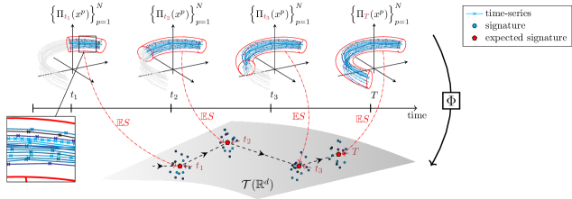
that maps any path $x$ to its restriction to the sub-interval $[a,t]\subset I$, such that $\Pi_{t}(x)=x_{|_{[a,t]}}$ (see Figure 2).

Definition 3.2.

The pathwise expected signature is the function $\Phi:\mathcal{P}(\mathcal{X})\to\mathcal{C}(I,\mathcal{T}(E))$ that to a probability measure $\mu\in\mathcal{P}(\mathcal{X})$ associates the path $\Phi(\mu):I\to\mathcal{T}(E)$ defined as

$$\Phi(\mu):t\mapsto\mathbb{E}_{x\sim\mu}\left[S\left(\Pi_{t}(x)\right)\right].$$ (12)

The action of the function $\Phi$ is illustrated on Figure 2, and its implementation is outlined in Algorithm 1.

Algorithm 1 Pathwise Expected Signature (PES)

1:Input: $N$ streams $\{\mathbf{x}^{p}\}_{p=1}^{N}$ each of length $\ell$

2:Create array $\Phi$ to store the PES

3:Create array $S$ to store the signatures

4:Initialize $S[p]\leftarrow 1$ for $p\in\{1,\ldots,N\}$

5:for each time-step $k\in\{2,\ldots,\ell\}$ do

6:     $S[p]\leftarrow S[p]\otimes\exp(\mathbf{x}^{p}_{k}-\mathbf{x}^{p}_{k-1})$ for $p\in\{1,\ldots,N\}$

7:     $\Phi[k]\leftarrow\mathrm{avg}(S)$

8:Output: The pathwise expected signature $\Phi$

In line $6$ of the algorithm we use an algebraic property for fast computation of the signature, known as Chen’s relation (detailed in Appendix).

The next theorem states that any weakly continuous function on $\mathcal{P}(\mathcal{X})$ can be uniformly well approximated by a linear combination of terms in the signature of the pathwise expected signature.

Theorem 3.2.

Let $\mathcal{X}\subset\mathcal{C}(I,E)$ be a compact set of paths and consider a weakly continuous function $F:\mathcal{P}(\mathcal{X})\to\mathbb{R}$. Then for any $\epsilon>0$ there exists a truncation level $m\geq 0$ such that for any probability measure $\mu\in\mathcal{P}(\mathcal{X})$

$$\Big{|}F(\mu)-\sum_{k=0}^{m}\sum_{J\in\{1,\ldots,d\}^{k}}\alpha_{J}S(\Phi(\mu))^{J}\Big{|}<\epsilon,$$ (13)

where $\alpha_{J}\in\mathbb{R}$ are scalar coefficients.

Proof.

$\mathcal{P}(\mathcal{X})$ is compact (see proof of Theorem 3.3) and the image of a compact set by a continuous function is compact. Therefore, the image $K=\Phi(\mathcal{P}(\mathcal{X}))$ is a compact subset of $\mathcal{C}(I,\mathcal{T}(E))$. Consider a weakly continuous function $F:\mathcal{P}(\mathcal{X})\to\mathbb{R}$. Given that $\Phi$ is injective (see Appendix), $\Phi$ is a bijection when restricted to its image $K$. Hence, there exists a continuous function $f:K\to\mathbb{R}$ (w.r.t $\left\lVert\cdot\right\rVert_{Lip}$) such that $F=f\circ\Phi$. By Theorem 2.1 we know that for any $\epsilon>0$, there exists a linear functional $\mathcal{L}:\mathcal{T}(E)\to\mathbb{R}$ such that $\left\lVert f-\mathcal{L}\circ S\right\rVert_{\infty}<\epsilon$. Thus $\|F\circ\Phi^{-1}-\mathcal{L}\circ S\|_{\infty}<\epsilon$, implying $\|F-\mathcal{L}\circ S\circ\Phi\|_{\infty}<\epsilon$. ∎

The practical consequence of this theorem is that the complex task of learning a highly non-linear regression function $F:P(\mathcal{X})\to\mathbb{R}$ can be reformulated as a linear regression on the signature (truncated at level $m$) of the pathwise expected signature (truncated at level $n$). The resulting ses algorithm is outlined in Alg.2, and has time complexity $\mathcal{O}(M\ell d^{n}(N+d^{m}))$, where $M$ is the total number of groups, $\ell$ is the largest length across all time-series, $d$ is the state space dimension, $N$ is the maximum number of input time series in a single group and $n,m$ are the truncation levels of the signature and pathwise expected signature respectively.

Algorithm 2 dr on sequential data with ses

1:Input: $\{(\{\mathbf{x}^{i,p}\}_{p=1}^{N_{i}},y^{i})\}_{i=1}^{M}$

2:Create array $A$ to store $M$ signatures of the PES.

3:for  each group $i\in\{1,...,M\}$ do

4:     $\Phi=\mathrm{PES}(\{\mathbf{x}^{i,p}\}_{p=1}^{N_{i}})$          // Using Algorithm 1

5:     for each time-step $k\in\{2,\ldots,\ell_{i}\}$ do

6:         // Compute the signature of the PES

7:         // via Chen’s relation

8:         $A[:,i]\leftarrow A[:,i]\otimes\exp{(\Phi_{k}-\Phi_{k-1})}$      

9:$(\alpha_{0},\ldots,\alpha_{c})$ $\leftarrow$ LinearRegression($A,(y^{i})_{i=1}^{M}$)

10:Output: Regression coefficients $(\alpha_{0},\ldots,\alpha_{c})$

3.2 A kernel-based approach (kes)

The ses algorithm is well suited to datasets containing a possibly large number $MN$ of relatively low dimensional paths. If instead the input paths are high dimensional, it would be prohibitive to deploy ses since the number of terms in the signature increases exponentially in the dimension $d$ of the path. To address this, in this section we construct a new kernel function $k:\mathcal{P}(\mathcal{X})\times\mathcal{P}(\mathcal{X})\to\mathbb{R}$ combining the expected signature with a Gaussian kernel and prove its universality to approximate weakly continuous function on probability measures on paths. The resulting kernel-based algorithm (kes) for dr on sequential data is well-adapted to the opposite data regime to the one above, i.e. when the dataset consists of few number $MN$ of high dimensional paths.

Theorem 3.3.

Let $\mathcal{X}\subset\mathcal{C}(I,E)$ be a compact set of paths and $\sigma>0$. The kernel $k:\mathcal{P}(\mathcal{X})\times\mathcal{P}(\mathcal{X})\to\mathbb{R}$ defined by

$$k(\mu,\nu)=\exp{\Big{(}-\sigma^{2}\left\lVert\mathbb{E}S(\mu)-\mathbb{E}S(\nu)\right\rVert_{\mathcal{T}(E)}^{2}\Bigr{)}},$$ (14)

is universal, i.e. the associated RKHS is dense in the space of continuous functions from $\mathcal{P}(\mathcal{X})$ to $\mathbb{R}$.

Proof.

By Christmann and Steinwart, (2010, Thm. 2.2) if $K$ is a compact metric space and $H$ is a separable Hilbert space such that there exists a continuous and injective map $\rho:K\to H$, then for $\sigma>0$ the Gaussian-type kernel $k_{\sigma}:K\times K\to\mathbb{R}$ is a universal kernel, where $k_{\sigma}(z,z^{\prime})=\exp{\Big{(}-\sigma^{2}\left\lVert\rho(z)-\rho(z^{\prime})\right\rVert_{H}^{2}\Bigr{)}}$. With the metric induced by $\left\lVert\cdot\right\rVert_{Lip},\mathcal{X}$ is a compact metric space. Hence the set $\mathcal{P}(\mathcal{X})$ is weakly-compact (Walkden,, 2014, Thm. 10.2). By Theorem 3.1, the expected signature $\mathbb{E}S:\mathcal{P}(\mathcal{X})\to\mathcal{T}(E)$ is injective and weakly continuous. Furthermore $\mathcal{T}(E)$ is a Hilbert space with a countable basis, hence it is separable. Setting $K=\mathcal{P}(\mathcal{X}),H=\mathcal{T}(E)$ and $\rho=\mathbb{E}S$ concludes the proof. ∎

3.3 Evaluating the universal kernel $k$

When the input measures are two empirical measures $\delta^{1}=\frac{1}{N_{1}}\sum_{p=1}^{N_{1}}\delta_{x^{1,p}}$ and $\delta^{2}=\frac{1}{N_{2}}\sum_{q=1}^{N_{2}}\delta_{x^{2,q}}$, the evaluation of the kernel $k$ in Equation 14 requires the ability to compute the tensor norm on $\mathcal{T}(E)$

$$\left\lVert\mathbb{E}S(\delta^{1})-\mathbb{E}S(\delta^{2})\right\rVert^{2}=E_{11}+E_{22}-2E_{12},$$

$$E_{ij}=\frac{1}{N_{i}N_{j}}\sum_{p,q=1}^{N_{i},N_{j}}\bigl{\langle}S(x^{i,p}),S(x^{j,q})\bigr{\rangle},~{}i,j\in\{1,2\}$$ (15)

where all the inner products are in $\mathcal{T}(E)$. Each of these inner products defines another recent object from stochastic analysis called the signature kernel $k_{sig}$ (Király and Oberhauser,, 2019). Recently, Cass et al., (2020) have shown that $k_{sig}$ is actually the solution of a surprisingly simple partial differential equation (PDE). This result provides us with a “kernel trick” for computing the inner products in Section 3.3 by a simple call to any numerical PDE solver of choice.

Theorem 3.4.

(Cass et al.,, 2020, Thm. 2.2) The signature kernel defined as

$$k_{sig}(x,y):=\langle S(x),S(y)\rangle_{\mathcal{T}(E)}$$ (16)

is the solution $u:[a,T]\times[a,T]\to\mathbb{R}$ at $(s,t)=(T,T)$ of the following linear hyperbolic PDE

$$\frac{\partial^{2}u}{\partial s\partial t}=(\dot{x}_{s}^{T}\dot{y}_{t})u u(a,\cdot)=1,~{}u(\cdot,a)=1.$$ (17)

In light of Theorem 3.3, dr on paths with kes can be performed via any kernel method (Drucker et al.,, 1997; Quiñonero-Candela and Rasmussen,, 2005) available within popular libraries (Pedregosa et al.,, 2011; De G. Matthews et al.,, 2017; Gardner et al.,, 2018) using the Gram matrix computed via Algorithm 3 and leveraging the aforementioned kernel trick. When using a finite difference scheme (referred to as PDESolve in Algorithm 3) to approximate the solution of the PDE, the resulting time complexity of kes is $\mathcal{O}(M^{3}+M^{2}N^{2}\ell^{2}d)$.

Algorithm 3 Gram matrix for kes

1:Input: $\{x^{i,p}\}_{p=1}^{N_{i}},~{}i=1,\ldots,M$ and $\sigma>0$.

2:Initialize $0$-array $G\in\mathbb{R}^{M\times M}$

3:for each pair of groups $(i,j)$ such that $i\leq j$ do

4:     Initialize $0$-array $K_{ij}\in\mathbb{R}^{N_{i}\times N_{j}}$

5:     Similarly initialize $K_{ii},K_{jj}\in\mathbb{R}^{N_{i}\times N_{i}},\mathbb{R}^{N_{j}\times N_{j}}$

6:     for $p,p^{\prime}$ in group $i$ and $q,q^{\prime}$ in group $j$ do

7:         $K_{ii}[p,p^{\prime}]\leftarrow\mathrm{PDESolve}(x^{i,p},x^{i,p^{\prime}})$

8:         $K_{jj}[q,q^{\prime}]\leftarrow\mathrm{PDESolve}(x^{j,q},x^{j,q^{\prime}})$

9:         $K_{ij}[p,q]\leftarrow\mathrm{PDESolve}(x^{i,p},x^{j,q})$      

10:     $G[i,j]\leftarrow\mathrm{avg}(K_{ii})+\mathrm{avg}(K_{jj})-2\times\mathrm{avg}(K_{ij})$

11:     $G[j,i]\leftarrow G[i,j]$

12:$G\leftarrow\exp(-\sigma^{2}G)$          // element-wise $exp$

13:Output: The gram matrix $G$.

Remark

In the case where the observed paths are assumed to be i.i.d. samples $\{x^{p}\}_{p=1}^{N}\sim\mu$ from the law of an underlying random process one would expect the bigger the sample size $N$, the better the approximation of $\mu$, and therefore of its expected signature $\mathbb{E}S(\mu)$. Indeed, for an arbitrary multi-index $\tau=(i_{1},\ldots,i_{k})$, the Central Limit Theorem yields the convergence (in distribution)

$$\sqrt{N}\Bigl{(}\mathbb{E}_{x\sim\mu}[S^{\tau}(x)]-\frac{1}{N}\sum_{p=1}^{N}S^{\tau}(x^{p})\Bigr{)}\overset{\mathcal{D}}{\to}\mathcal{N}(0,\sigma_{\tau}^{2})$$

as the variance $\sigma_{\tau}^{2}=\mathbb{E}_{x\sim\mu}[S^{\tau}(x)^{2}]-(\mathbb{E}_{x\sim\mu}[S^{\tau}(x)])^{2}$ is always finite; in effect for any path $x$, the product $S^{\tau}(x)S^{\tau}(x)$ can always be expressed as a finite sum of higher-order terms of $S(x)$ (Chevyrev and Kormilitzin,, 2016, Thm. 1).

4 RELATED WORK

Recently, there has been an increased interest in extending regression algorithms to the case where inputs are sets of numerical arrays (Hamelijnck et al.,, 2019; Law et al.,, 2018; Musicant et al.,, 2007; Wagstaff et al.,, 2008; Skianis et al.,, 2019). Here we highlight the previous work most closely related to our approach.

Deep learning techniques

DeepSets (Zaheer et al.,, 2017) are examples of neural networks designed to process each item of a set individually, aggregate the outputs by means of well-designed operations (similar to pooling functions) and feed the aggregated output to a second neural network to carry out the regression. However, these models depend on a large number of parameters and results may largely vary with the choice of architecture and activation functions (Wagstaff et al.,, 2019).

Kernel-based techniques

In the setting of dr, elements of a set are viewed as samples from an underlying probability distribution (Szabó et al.,, 2016; Law et al.,, 2017; Muandet et al.,, 2012; Flaxman,, 2015; Smola et al.,, 2007). This framework can be intuitively summarized as a two-step procedure. Firstly, a probability measure $\mu$ is mapped to a point in an RKHS $\mathcal{H}_{1}$ by means of a kernel mean embedding $\Phi:\mu\to\int_{x\in\mathcal{X}}k_{1}(\cdot,x)\mu(dx)$, where $k_{1}:\mathcal{X}\times\mathcal{X}\to\mathbb{R}$ is the associated reproducing kernel. Secondly, the regression is finalized by approximating a function $F:\mathcal{H}_{1}\to\mathbb{R}$ via a minimization of the form $F\approx\operatorname*{arg\,min}_{g\in\mathcal{H}_{2}}\sum_{i=1}^{M}\mathcal{L}(y^{i},g\circ\Phi(\mu^{i}))$, where $\mathcal{L}$ is a loss function, resulting in a procedure involving a second kernel $k_{2}:\mathcal{H}_{1}\times\mathcal{H}_{1}\to\mathbb{R}$. Despite the theoretical guarantees of these methods (Szabó et al.,, 2016), the feature map $k_{1}(\cdot,x)$ acting on the support $\mathcal{X}$ is rarely provided explicitly, especially in the setting of non-standard input spaces $\mathcal{X}\not\subset\mathbb{R}^{d}$, requiring manual adaptations to make the data compatible with standard kernels. In Section 5 we denote by DR-$k_{1}$ the models produced by choosing $k_{2}$ to be a Gaussian-type kernel.

The signature method

The signature method consists in using the terms of the signature as features to solve supervised learning problems on time-series, with successful applications for detection of bipolar disorder (Arribas et al.,, 2018) and human action recognition (Yang et al.,, 2017) to name a few. The signature features have been used to construct neural network layers (Bonnier et al.,, 2019; Graham,, 2013) in deep architectures. To the best of our knowledge, we are the first to use signatures in the context of dr.

5 EXPERIMENTS

We benchmark our feature-based (ses) and kernel-based (kes) methods against DeepSets and the existing kernel-based dr techniques discussed in Section 4 on various simulated and real-world examples from physics, mathematical finance and agricultural science. With these examples, we show the ability of our methods to handle challenging situations where only a few number of labelled groups of multivariate time-series are available. We consider the kernel-based techniques DR-$k_{1}$ with $k_{1}\in\{\mathrm{RBF},\mathrm{Matern32},\mathrm{GA}\}$, where GA refers to the Global Alignment kernel for time-series from Cuturi et al., (2007). For kes and DR-$k_{1}$ we perform Kernel Ridge Regression, whilst for ses we use Lasso Regression. All models are run $5$ times and we report the mean and standard deviation of the predictive mean squared error (MSE). Other metrics are reported in the Appendix. The hyperparameters of kes, ses and DR-$k_{1}$ are selected by cross-validation via a grid search on the training set of each run. Additional details about hyperparameters search and model architecture, as well as the code to reproduce the experiments can be found in the supplementary material.

5.1 A defective electronic device

We start with a toy example to show the robustness of our methods to irregularly sampled time-series.

Figure 3: Predictive MSE at various subsampling rates for $M=50$ circuits and $N=15$ devices. The shaded area indicates the standard deviation.

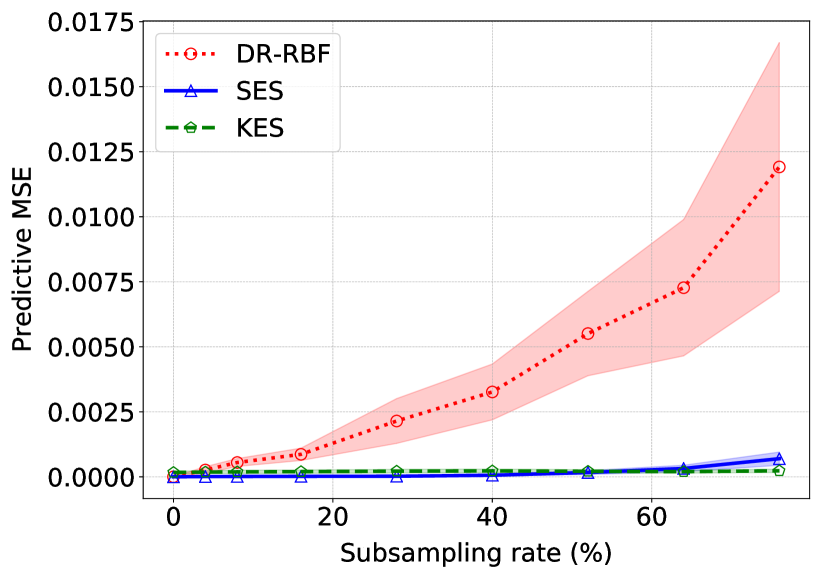
For this, we propose to infer the phase $\varphi$ of an electronic circuit from multiple recordings of its voltage $v^{\varphi}(t)=\sin(\omega t)$ and current $i^{\varphi}(t)=\sin(\omega t-\varphi)$. The data consists of $M$ simulated circuits with phases $\{\varphi^{i}\}_{i=1}^{M}$ selected uniformly at random from $[\pi/8,\pi/2]$. Each circuit is attached to $N$ measuring devices recording the two sine waves over $20$ periods at a frequency $25$ points per period. We then randomly subsample the data at rates ranging from $0\%$ to $75\%$ independently for each defective device. As shown in Figure 3, the predictive performances of DR-RBF drastically deteriorate when the subsampling rate increases, whilst results for kes and ses remain roughly unchanged.

5.2 Inferring the temperature of an ideal gas

Table 1: Ideal gas dataset. Radii of all particles composing the simulated gases: $r_{1}=3.5\cdot 10^{-1}(V/N)^{3}$ (few collisions) and $r_{2}=6.5\cdot 10^{-1}(V/N)^{3}$ (many collisions).

Model	Predictive MSE [$\times 10^{-2}$]
	$r_{1}$	$r_{2}>r_{1}$
DeepSets	8.69 (3.74)	5.61 (0.91)
DR-RBF	3.08 (0.39)	4.36 (0.64)
DR-Matern32	3.54 (0.48)	4.12 (0.39)
DR-GA	2.85 (0.43)	3.69 (0.36)
1-3        kes		1.31 (0.34)	0.08 (0.02)
ses	1.26 (0.23)	0.09 (0.03)

The thermodynamic properties of an ideal gas of $N$ particles inside a $3$-d box of volume $V$ ($3$ cm3) can be described in terms of the temperature $T$ (K), the pressure $P$ (Pa) and the total energy $U$ (J) via the two equations of state $PV=Nk_{B}T$ and $U=c_{V}Nk_{B}T$, where $k_{B}$ is the Boltzmann constant (Adkins and Adkins,, 1983), and $c_{V}$ the heat capacity. The large-scale behaviour of the gas can be related to the trajectories of the individual particles (through their momentum = mass $\times$ velocity) by the equation $U=\frac{1}{2}\sum_{p=1}^{N}m_{p}|\vv{v_{p}}|^{2}$. The complexity of the large-scale dynamics of the gas depends on $T$ (see Figure 1) as well as on the radius of the particles. For a fixed $T$, the larger the radius the higher the chance of collision between the particles. We simulate $M=50$ different gases of $N=20$ particles each by randomly initialising all velocities and letting particles evolve at constant speed. The task is to learn $T$ (sampled uniformly at random from $[1,1\,000]$) from the set of trajectories traced by the particles in the gas. In Table 5.2 we report the results of two experiments, one where particles have a small radius (few collisions) and another where they have a bigger radius (many collisions). The performance of DR-$k_{1}$ is comparable to the ones of kes and ses in the simpler setting. However, in the presence of a high number of collisions our models become more informative to retrieve the global temperature from local trajectories, whilst the performance of DR-$k_{1}$ drops with the increase in system-complexity. With a total number of $MN=1\,000$ time-series of dimension $d=7$ (after path augmentation discussed in Section 2.5 and in the Appendix), kes runs in $50$ seconds, three times faster than ses on a $128$ cores CPU.

5.3 Parameter estimation in a pricing model

Table 2: Predictive MSE (standard deviation) on the rough volatility dataset. $N$ is the number of rough volatility trajectories and $(M,d,\ell)=(50,2,200)$.

Model	Predictive MSE [$\times 10^{-3}$]
	N=20	N=50	N=100
DeepSets	74.43 (47.57)	74.07 (49.15)	74.03 (47.12)
DR-RBF	52.25 (11.20)	58.71 (19.05)	44.30 (7.12)
DR-Matern32	48.62 (10.30)	54.91 (12.02)	32.99 (5.08)
DR-GA	3.17 (1.59)	2.45 (2.73)	0.70 (0.42)
1-4        kes		1.41 (0.40)	0.30 (0.07)	0.16 (0.03)
ses	1.49 (0.39)	0.33 (0.12)	0.21 (0.05)

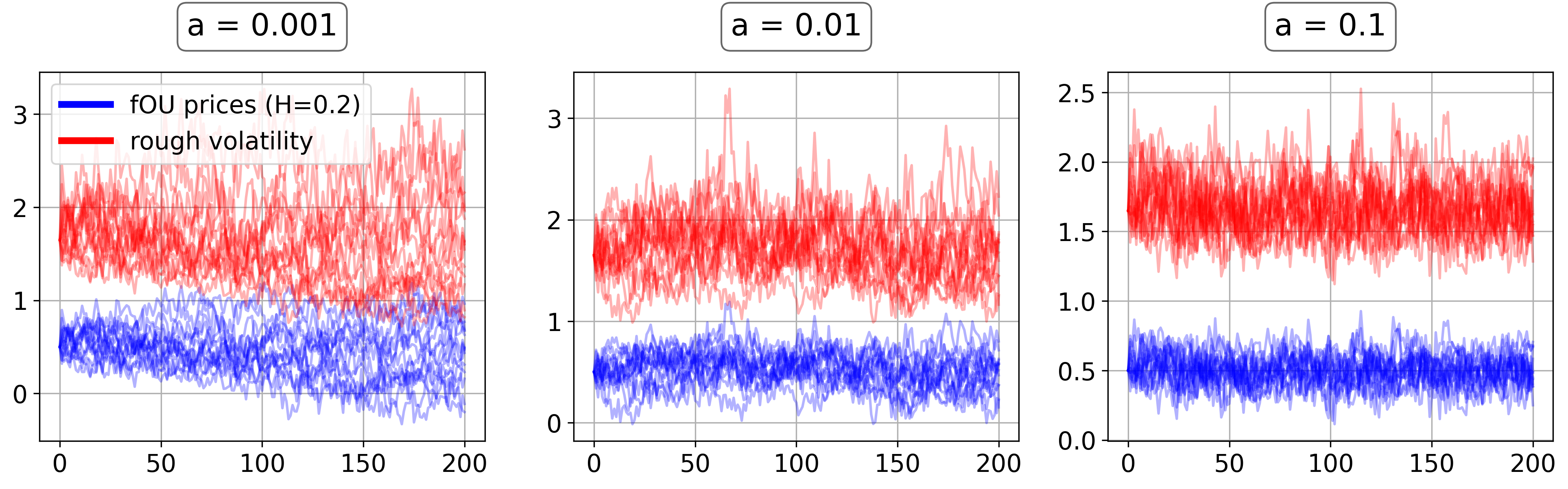
Financial practitioners often model asset prices via an SDE of the form $dP_{t}=\mu_{t}dt+\sigma_{t}dW_{t}$, where $\mu_{t}$ is a drift term, $W_{t}$ is a $1$-d Brownian motion (BM) and $\sigma_{t}$ is the volatility process (Arribas et al.,, 2020). This setting is often too simple to match the volatility observed in the market, especially since the advent of electronic trading (Gatheral et al.,, 2018). Instead, we model the (rough) volatility process as $\sigma_{t}=\exp\{P_{t}\}$ where $dP_{t}=-a(P_{t}-m)dt+\nu dW_{t}^{H}$ is a fractional Ornstein-Uhlenbeck (fOU) process, with $a,\nu,m$ $\geq$ $0$. The fOU is driven by a fractional Brownian Motion (fBM) $W_{t}^{H}$ of Hurst exponent $H\in(0,1)$, governing the regularity of the trajectories (Decreusefond et al.,, 1999). In line with the findings in Gatheral et al., (2018) we choose $H=0.2$ and tackle the task of estimating the mean-reversion parameter $a$ from simulated sample-paths of $\sigma_{t}$. We consider $50$ mean-reversion values $\{a^{i}\}_{i=1}^{50}$ chosen uniformly at random from $[10^{-6},1]$. Each $a^{i}$ is regressed on a collection of $N=20,50,100$ (time-augmented) trajectories $\{\hat{\sigma}_{t}^{i,p}\}_{p=1}^{N}$ of length $200$. As shown in Table 5.3, kes and ses systematically yield the best MSE among all compared models. Moreover, the performance of kes and ses progressively improves with the number of time series in each group, in accordance to the remark at the end of Section 3, whilst this pattern is not observed for DR-RBF, DR-Matern32, and DeepSets. Both kes and ses yield comparable performances. However, whilst the running time of ses remains stable ($\approx 1~{}\mathrm{min}$) when $MN$ increases from $1\,000$ to $5\,000$, the running time of kes increases from $\approx 1~{}\mathrm{min}$ to $15~{}\mathrm{min}$ (on $128$ cores).

5.4 Crop yield prediction from GLDAS data

Finally, we evaluate our methods on a crop yield prediction task. The challenge consists in predicting the yield of wheat crops over a region from the longitudinal measurements of climatic variables recorded across different locations of the region. We use the publicly available Eurostat dataset containing the total annual regional yield of wheat crops in mainland France—divided in $22$ administrative regions—from $2015$ to $2017$. The climatic measurements (temperature, soil humidity and precipitation) are extracted from the GLDAS database (Rodell et al.,, 2004), are recorded every $6$ hours at a spatial resolution of $0.25$\mathrm{\SIUnitSymbolDegree}$\times 0.25$\mathrm{\SIUnitSymbolDegree}$$, and their number varies across regions. We further subsample at random $50\%$ of the measurements. ses and kes are the two methods which improve the most against the baseline which consists in predicting the average yield on the train set (Table LABEL:table:crops).

Table 3: MSE and MAPE (mean absolute percentage error) on the Eurostat/GLDAS dataset

Model	MSE	MAPE
Baseline	2.38 (0.60)	23.31 (4.42)
1-3 DeepSets	2.67 (1.02)	22.88 (4.99)
DR-RBF	0.82 (0.22)	13.18 (2.52)
DR-Matern32	0.82 (0.23)	13.18 (2.53)
DR-GA	0.72 (0.19)	12.55 (1.74)
1-3        kes		0.65 (0.18)	12.34 (2.32)
ses	0.62 (0.10)	10.98 (1.12)

6 CONCLUSION

We have developed two novel techniques for distribution regression on sequential data, a task largely ignored in the previous literature. In the first technique, we introduce the pathwise expected signature and construct a universal feature map for probability measures on paths. In the second technique, we define a universal kernel based on the expected signature. We have shown the robustness of our proposed methodologies to irregularly sampled multivariate time-series, achieving state-of-the-art performances on various dr problems for sequential data. Future work will focus on developing algorithms to handle simultaneously a large number of groups of high-dimensional time-series.

Acknowledgments

We deeply thank Dr Thomas Cass and Dr Ilya Chevyrev for the very helpful discussions. ML was supported by the OxWaSP CDT under the EPSRC grant EP/L016710/1. CS was supported by the EPSRC grant EP/R513295/1. ML and TD were supported by the Alan Turing Institute under the EPSRC grant EP/N510129/1. CS and TL were supported by the Alan Turing Institute under the EPSRC grant EP/N510129/1.

Appendix A PROOFS

In this section, we prove that the expected signature $\mathbb{E}S$ is weakly continuous (Section A.1), and that the pathwise expected signature $\Phi$ is injective and weakly continuous (Section A.2).

Recall that in the main paper we consider a compact subset of paths $\mathcal{X}\subset\mathcal{C}(I,E)$, where $I$ is a closed interval and $E$ is a Banach space of dimension $d$ (possibly infinite, but countable). We will denote by $\mathcal{P}(\mathcal{X})$ the set of Borel probability measures on $\mathcal{X}$ and by $S(\mathcal{X})\subset\mathcal{T}(E)$ the image of $\mathcal{X}$ by the signature $S:\mathcal{C}(I,E)\to\mathcal{T}(E)$.

As shown in (Chevyrev and Oberhauser,, 2018, Section 3), if $E$ is a Hilbert space with inner product $\langle\cdot,\cdot\rangle_{E}$, then for any $k\geq 1$ the following bilinear form defines an inner product on $E^{\otimes k}$

$$\big{\langle}e_{i_{1}}\otimes\ldots\otimes e_{i_{k}},e_{j_{1}}\otimes\ldots\otimes e_{j_{k}}\big{\rangle}_{E^{\otimes k}}=\prod_{r=1}^{k}\delta_{i_{r},j_{r}},\hskip 14.22636pt\delta_{ij}=\begin{cases}1,&\text{if }i=j,\\ 0,&\text{if }i\neq j.\end{cases}$$ (18)

which extends by linearity to an inner product $\langle A,B\rangle_{\mathcal{T}(E)}=\sum_{k\geq 0}\langle A_{k},B_{k}\rangle_{E^{\otimes k}}$ on $\mathcal{T}(E)$ that thus becomes also a Hilbert space.

A.1 Weak continuity of the expected signature

Definition A.1.

A sequence of probability measures $\mu_{n}\in\mathcal{P}(\mathcal{X})$ converges weakly to $\mu$ if for every $f\in C_{b}(\mathcal{X},\mathbb{R})$ we have $\int_{\mathcal{X}}fd\mu_{n}\to\int_{\mathcal{X}}fd\mu$ as $n\to\infty$, where $C_{b}(\mathcal{X},\mathbb{R})$ is the space of real-valued continuous bounded functions on $\mathcal{X}$.

Remark.

Since $\mathcal{X}$ is a compact metric space, we can drop the word "bounded" in Definition A.1.

Definition A.2.

Given two probability measures $\mu,\nu\in\mathcal{P}(\mathcal{X})$, the Wasserstein-1 distance is defined as follows

$$W_{1}(\mu,\nu)=\inf_{\gamma\in\Pi(\mu,\nu)}\int_{x,y\in\mathcal{X}}\left\lVert x-y\right\rVert_{Lip}d\gamma(x,y)$$ (19)

where the infimum is taken over all possible couplings of $\mu$ and $\nu$.

Lemma A.1.

(Chevyrev and Oberhauser,, 2018, Theorem 5.3) The signature $S:\mathcal{C}(I,E)\to\mathcal{T}(E)$ is injective.

Lemma A.2.

(Chevyrev et al.,, 2016, Corollary 5.5) The signature $S:\mathcal{C}(I,E)\to\mathcal{T}(E)$ is continuous w.r.t. $\left\lVert\cdot\right\rVert_{Lip}$.

Lemma A.3.

(Chevyrev and Oberhauser,, 2018, Theorem 5.6) The expected signature $\mathbb{E}S:\mathcal{P}(\mathcal{X})\to\mathcal{T}(E)$ is injective.

Theorem A.1.

The expected signature $\mathbb{E}S:\mathcal{P}(\mathcal{X})\to\mathcal{T}(E)$ is weakly continuous.

Proof.

Consider a sequence $\{\mu_{n}\}_{n\in\mathbb{N}}$ of probability measures on $\mathcal{P}(\mathcal{X})$ converging weakly to a measure $\mu\in\mathcal{P}(\mathcal{X})$. By Lemma A.2 the signature $S:x\mapsto S(x)$ is continuous w.r.t. $\left\lVert\cdot\right\rVert_{Lip}$. Hence, by definition of weak-convergence (and because $\mathcal{X}$ is compact), for any $k>0$ and any multi-index $(i_{1},\ldots,i_{k})\in\{1,\ldots,d\}^{k}$ it follows that $\int_{x\in\mathcal{X}}S(x)^{(i_{1},\ldots,i_{k})}\mu_{n}(dx)\to\int_{x\in\mathcal{X}}S(x)^{(i_{1},\ldots,i_{k})}\mu(dx)$. The factorial decay given by (Lyons et al.,, 2007, Proposition 2.2) yields $\int_{x\in\mathcal{X}}S(x)\mu_{n}(dx)\to\int_{x\in\mathcal{X}}S(x)\mu(dx)$ in the topology induced by $\langle\cdot,\cdot\rangle_{\mathcal{T}(E)}$. ∎

A.2 Injectivity and weak continuity of the pathwise expected signature

Theorem A.2.

(Lyons et al.,, 2007, Theorem 3.7) Let $x\in\mathcal{C}(I,E)$ and recall the definition of the projection $\Pi_{t}:x\mapsto x_{|_{[a,t]}}$. Then, the $\mathcal{T}(E)$-valued path defined by

$$S_{path}(x):t\mapsto S\circ\Pi_{t}(x)$$ (20)

is Lipschitz continuous. Furthermore the map $x\mapsto S_{path}(x)$ is continuous w.r.t. $\left\lVert\cdot\right\rVert_{Lip}$.

Theorem A.3.

The pathwise expected signature $\Phi:\mathcal{P}(\mathcal{X})\to\mathcal{C}(I,\mathcal{T}(E))$ is injective.

Proof.

Let $\mu,\nu\in\mathcal{P}(\mathcal{X})$ be two probability measures. If $\Phi(\mu)=\Phi(\nu)$, then for any $t\in I$, $\mathbb{E}_{x\sim\mu}[S\circ\Pi_{t}(x)]=\mathbb{E}_{y\sim\nu}[S\circ\Pi_{t}(y)]$. In particular, for $t=T$, $\mathbb{E}S(\mu)=\mathbb{E}_{x\sim\mu}[S(x)]=\mathbb{E}_{y\sim\nu}[S(y)]=\mathbb{E}S(\nu)$. The result follows from the injectivity of the expected signature $\mathbb{E}S$ (Lemma A.3). ∎

Theorem A.4.

The pathwise expected signature $\Phi:\mathcal{P}(\mathcal{X})\to\mathcal{C}(I,\mathcal{T}(E))$ is weakly continuous.

Proof.

Let $\{\mu_{n}\}_{n\in\mathbb{N}}$ be a sequence in $\mathcal{P}(\mathcal{X})$ converging weakly to $\mu\in\mathcal{P}(\mathcal{X})$. As $S_{path}$ is continuous (Theorem A.2), it follows, by the continuous mapping theorem, that $S_{path}\#\mu_{n}\to S_{path}\#\mu$ weakly, where $S_{path}\#\mu$ is the pushforward measure of $\mu$ by $S_{path}$. Given that $S_{path}$ is continuous and $\mathcal{X}$ is compact, it follows that the image $S_{path}(\mathcal{X})$ is a compact subset of the Banach space $\mathcal{C}(I,\mathcal{T}(E))$. By (Villani,, 2008, Theorem 6.8) weak convergence of probability measures on compact supports is equivalent to convergence in Wasserstein-1 distance. By Jensen’s inequality $\left\lVert\mathbb{E}[S_{path}\#\mu_{n}]-\mathbb{E}[S_{path}\#\mu]\right\rVert_{Lip}\leq\mathbb{E}[\left\lVert S_{path}\#\mu_{n}-S_{path}\#\mu\right\rVert_{Lip}]$. Taking the infimum over all couplings $\gamma\in\Pi(S_{path}\#\mu_{n},S_{path}\#\mu)$ on the right-hand-side of the previous equation we obtain $\left\lVert\mathbb{E}[S_{path}\#\mu_{n}]-\mathbb{E}[S_{path}\#\mu]\right\rVert_{Lip}\leq W_{1}(S_{path}\#\mu_{n},S_{path}\#\mu)\to 0$, which yields the convergence $\mathbb{E}[S_{path}\#\mu_{n}]\to\mathbb{E}[S_{path}\#\mu]$ in $\left\lVert\cdot\right\rVert_{Lip}$ over $\mathcal{C}(I,\mathcal{T}(E))$. Noting that $\mathbb{E}[S_{path}\#\mu]=\Phi(\mu)$ concludes the proof. ∎

Appendix B EXPERIMENTAL DETAILS

In our experiments we benchmark kes and ses against DeepSets and DR-$k_{1}$ where $k_{1}\in\{\mathrm{RBF},\mathrm{Matern32},\mathrm{GA}\}$. Both kes and ses do not take into account the length of the input time-series. Apart from DR-GA, all other baselines are designed to operate on vectorial data. Therefore, in order to deploy them in the setting of dr on sequential data, manual pre-processing (such as padding) is required. In the next section we describe how we turn discrete time-series into continuous paths on which the signature operates.

B.1 Transforming discrete time-series into continuous paths

Consider a $d$-dimensional time-series of the form $\mathbf{x}=\{(t_{1},\mathbf{x}_{1}),\ldots,(t_{\ell},\mathbf{x}_{\ell})\}$ with time-stamps $t_{1}$ $\leq$ $\ldots$ $\leq$ $t_{\ell}$ and values $\mathbf{x}_{k}\in\mathbb{R}^{d}$, and the continuous path $x$ obtained by linearly interpolating between the points $\mathbf{x}_{1},\cdots,\mathbf{x}_{\ell}$. The signature (truncated at level $n$) of $x$ can be computed explicitly with existing Python packages Reizenstein and Graham, (2018); et al, (2010); Kidger and Lyons, (2020), does not depend on the time-stamps $(t_{1},\ldots,t_{\ell_{i,j}})$, and produces $(d^{n+1}-1)/(d-1)$ terms when $d>1$. When $d=1$ the signature is trivial since $S^{\leq n}(x)=(1,(x_{t_{\ell}}-x_{t_{1}}),\frac{1}{2}(x_{t_{\ell}}-x_{t_{1}})^{2},\cdots,\frac{1}{n!}(x_{t_{\ell}}-x_{t_{1}})^{n})$. As mentioned in Section 2.5 we can simply augment the paths with a monotonous coordinate, such that $\hat{x}:t\mapsto(t,x_{t})$, where $t\in[a,T]$, effectively reintroducing a time parametrization. Another way to augment the state space of the data and obtain additional signature terms is the lead-lag transformation (see Definition B.1) which turns a $1$-d data stream into a $2$-d path. For example if the data stream is $\{1,5,3\}$ one obtains the $2$-d continuous path $\hat{x}:t\mapsto(x_{t}^{(lead)},x_{t}^{(lag)})$ where $x^{(lead)}$ and $x^{(lag)}$ are the linear interpolations of $\{1,5,5,3,3\}$ and $\{1,1,5,5,3\}$ respectively. A key property of the lead-lag transform is that the difference between $S(\hat{x})^{(1,2)}$ and $S(\hat{x})^{(2,1)}$ is the quadratic variation $QV(x)=\sum_{k=1}^{\ell-1}(x_{t_{k+1}}-x_{t_{k}})^{2}$ Chevyrev and Kormilitzin, (2016). Hence, even when $d>1$, it may be of interest to lead-lag transform the coordinates of the paths for which the quadratic variation is important for the task at hand.

Definition B.1 (Lead-lag).

Given a sequence of points $\mathbf{x}=\{\mathbf{x}_{1},\ldots,\mathbf{x}_{\ell}\}$ in $\mathbb{R}^{d}$ the lead-lag transform yields two new sequences $\mathbf{x}^{(lead)}$ and $\mathbf{x}^{(lag)}$ of length $2\ell-1$ of the following form

$$\mathbf{x}^{(lead)}_{p}=\left\{\begin{array}[]{ll}\mathbf{x}_{k}&\mathrm{if}~{}p=2k-1\\ \mathbf{x}_{k}&\mathrm{if}~{}p=2k-2.\end{array}\right. \mathbf{x}^{(lag)}_{p}=\left\{\begin{array}[]{ll}\mathbf{x}_{k}&\mathrm{if}~{}p=2k-1\\ \mathbf{x}_{k}&\mathrm{if}~{}p=2k.\end{array}\right.$$

In our experiments we add time and lead-lag all coordinates except for the first task which consists in inferring the phase of an electronic circuit (see Section 5.1 in the main paper).

B.2 Implementation details

The distribution regression methods (including DR-$k_{1}$, kes and ses) are implemented on top of the Scikit-learn library Pedregosa et al., (2011), whilst we use the existing codebase https://github.com/manzilzaheer/DeepSets for DeepSets.

B.2.1 KES

The kes algorithm relies on the signature kernel trick which is referred to as PDESolve in the main paper. In the algorithm below we outline the finite difference scheme we use for the experiments. In all the experiments presented in the main paper, the discretization level of the PDE solver is fixed to $n=0$ such that the time complexity to approximate the solution of the PDE is $\mathcal{O}(d\ell^{2})$ where $\ell$ is the length of the longest data stream.

Algorithm 4 PDESolve

1:Input: two streams $\{\mathbf{x}_{k}\}_{k=1}^{\ell_{\mathbf{x}}}$, $\{\mathbf{y}_{k}\}_{k=1}^{\ell_{\mathbf{y}}}$ of dimension $d$ and discretization level $n$ (step size $=2^{-n}$)

2:Create array $U$ to store the solution of the PDE

3:Initialize $U[i,:]\leftarrow 1$ for $i\in\{1,2,\ldots,2^{n}*(\ell_{x}-1)+1\}$

4:Initialize $U[:,j]\leftarrow 1$ for $j\in\{1,2,\ldots,2^{n}*(\ell_{y}-1)+1\}$

5:for each $i\in\{1,2,\ldots,2^{n}*(\ell_{\mathbf{x}}-1)\}$ do

6:     for each $j\in\{1,2,\ldots,2^{n}*(\ell_{\mathbf{y}}-1)\}$ do

7:         $\Delta_{\mathbf{x}}=(\mathbf{x}_{\left\lceil i/(2^{n})\right\rceil+1}-\mathbf{x}_{\left\lceil i/(2^{n})\right\rceil})/2^{n}$

8:         $\Delta_{\mathbf{y}}=(\mathbf{y}_{\left\lceil j/(2^{n})\right\rceil+1}-\mathbf{y}_{\left\lceil j/(2^{n})\right\rceil})/2^{n}$

9:         $U[i+1,j+1]=U[i,j+1]+U[i+1,j]+(\Delta_{\mathbf{x}}^{T}\Delta_{\mathbf{y}}-1.)*U[i,j]$      

10:Output: The solution of the PDE at the final times $U[-1,-1]$

B.2.2 SES

The ses algorithm from the main paper relies on an algebraic property for fast computation of signatures, known as Chen’s relation. Given a piecewise linear path $x=\Delta x_{t_{2}}\star\ldots\star\Delta x_{t_{\ell}}$ given by the concatenation $\star$ of individual increments $\mathbb{R}^{d}\ni\Delta x_{t_{k}}=x_{t_{k}}-x_{t_{k-1}},~{}k=2,\ldots,\ell$, one has $S(x)=\exp(\Delta x_{t_{2}})\otimes\ldots\otimes\exp(\Delta x_{t_{\ell}})$, where $\exp$ denotes the tensor exponential and $\otimes$ the tensor product. Using Chen’s relation, computing the signature (truncated at level $n$) of a sequence of length $\ell$ has complexity $\mathcal{O}(\ell d^{n})$.

B.2.3 Baselines

Table 4: Kernels $k_{1}$ for the kernel-based baselines. See Cuturi and Blondel, (2017) for the definition of $\mathrm{dtw}_{1/\gamma}$ in the GA kernel.

RBF	$\exp(-\gamma^{2}\left\lVert x-x^{\prime}\right\rVert^{2})$
Matern32	$(1+\sqrt{3}\gamma^{2}\left\lVert x-x^{\prime}\right\rVert)\exp(-\sqrt{3}\gamma^{2}\left\lVert x-x^{\prime}\right\rVert)$
GA	$\exp(-\gamma\,\mathrm{dtw}_{1/\gamma}(x,x^{\prime}))$

For the kernel-based baselines DR-$k_{1}$, we perform Kernel Ridge regression with the kernel defined by $k(\delta^{i},\delta^{j})=\exp{(-\sigma^{2}\left\lVert\rho(\delta^{i})-\rho(\delta^{j})\right\rVert_{\mathcal{H}_{1}}^{2})}$, where $\rho(\delta^{i})=N_{i}^{-1}\sum_{p=1}^{N_{i}}k_{1}(\cdot,x^{i,p})$. For $k_{1}\in\{\mathrm{RBF},\mathrm{Matern32}\}$, if the time-series are multi-dimensional, the dimensions are stacked to form one large vector $x\in\mathbb{R}^{d\ell}$. See Table 1 for the expressions of the kernels $k_{1}$ used as baselines.

For DeepSets, the two neural networks are feedforward neural networks with ELU activations. We train by minimizing the mean squared error.

B.3 Hyperparameter selection

All models are run $5$ times. The hyperparameters of kes, ses and DR-$k_{1}$ are selected by cross-validation via a grid search on the training set ($80\%$ of the data selected at random) of each run. The range of values for each parameter is specified in Table 5.

Table 5: Range of values for each parameter of DR-$k_{1}$, kes and ses. We denote by $\alpha$ the regularization parameter in Kernel Ridge regression and Lasso regression. The kernels parameters $\gamma$ and $\sigma$ are expressed in terms of lengthscales $\ell_{1}$ and $\ell_{2}$ such that $\gamma^{2}=1/(2\ell_{1}^{2})$ and $\sigma^{2}=1/(2\ell_{2}^{2})$.

Model	$\ell_{1}$	$\ell_{2}$	$\alpha$	$n$	$m$
DR-RBF	$\{10^{-3},10^{-2},\ldots,10^{2},10^{3}\}$	$\{10^{-3},10^{-2},\ldots,10^{2},10^{3}\}$	$\{10^{-3},10^{-2},\ldots,10^{2},10^{3}\}$	N/A	N/A
DR-Matern32	$\{10^{-3},10^{-2},\ldots,10^{2},10^{3}\}$	$\{10^{-3},10^{-2},\ldots,10^{2},10^{3}\}$	$\{10^{-3},10^{-2},\ldots,10^{2},10^{3}\}$	N/A	N/A
DR-GA	$\{7\cdot 10^{1},7\cdot 10^{2}\}$	$\{10^{-3},10^{-2},\cdots,10^{2},10^{3}\}$	$\{10^{-3},10^{-2},\ldots,10^{2},10^{3}\}$	N/A	N/A
kes	N/A	$\{10^{-3},10^{-2},\ldots,10^{2},10^{3}\}$	$\{10^{-3},10^{-2},\ldots,10^{2},10^{3}\}$	N/A	N/A
ses	N/A	N/A	$\{10^{-5},10^{-4},\ldots,10^{4},10^{5}\}$	$\{2,3\}$	$\{2\}$

Appendix C ADDITIONAL RESULTS

C.1 Additional performance metrics

We report the mean absolute percentage error (MAPE) as well as the computational time on two synthetic examples (the ideal gas and the rough volatility examples). As discussed in the main paper, these two datasets represent two data regimes: in one case (the rough volatility model) there is a high number of low dimensional time-series (see Figure 4), whist in the other case (ideal gas), there is a relatively small number of time-series with a higher state-space dimension. Apart from DeepSets (which is run on a GPU), all other models are run on a $128$ cores CPU.

Figure 4: fOU sample-paths and corresponding volatility for $3$ different mean-reversion parameters.

Table 6: Ideal gas example.

Model	Predictive MAPE		Time (s)
	$r_{1}$	$r_{2}>r_{1}$
DeepSets	82.50 (20.20)	53.49 (13.93)	31
DR-RBF	32.09 (5.78)	41.15 (11.81)	58
DR-Matern32	33.79 (5.16)	40.20 (12.45)	55
DR-GA	31.61 (5.60)	39.17 (13.87)	68
1-4        kes		16.57 (4.86)	4.20 (0.79)	49
ses	15.75 (2.65)	4.44 (1.36)	120

Table 7: Rough volatility example.

Model	Predictive MAPE			Time (min)
	N=20	N=50	N=100	N=20	N=50	N=100
DeepSets	44.85 (17.80)	44.75 (17.93)	45.00  (18.21)	1.31	1.86	2.68
DR-RBF	43.86 (13.36)	45.54 (10.05)	41.00 (12.98)	0.71	1.38	7.50
DR-Matern32	40.97 (10.81)	43.59 (9.79)	35.35 (9.18)	0.73	1.00	7.80
DR-GA	11.94 (7.14)	9.54 (6.85)	5.51 (2.78)	0.68	2.60	9.80
1-7        kes		6.12 (1.00)	2.83 (0.49)	2.07 (0.42)	0.71	4.00	15.50
ses	6.67 (3.35)	3.58 (0.84)	2.14 (0.62)	0.60	0.65	0.78

C.2 Interpretability

Figure 5: The $5$ most predictive features provided by (Lasso) ses for the task of crop yield prediction.

When dealing with complex data-streams, cause-effect relations between the different path-coordinates might be an essential feature that one wishes to extract from the signal. Intrinsic in the definition of the signature is the concept of iterated integral of a path over an ordered set of time indices $a<u_{1}<\ldots<u_{k}<T$. This ordering of the domain of integration, naturally captures causal dependencies between the coordinate-paths $x^{(i_{1})},\ldots,x^{(i_{k})}$.

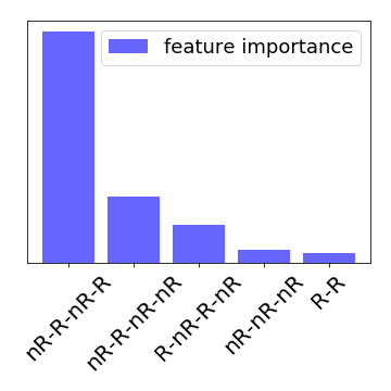
Taking this property into account, we revisit the crop yield prediction example (see Section 5.4 in the main paper, and Figure 6) to show how the iterated integrals from the signature (of the pathwise expected signature) provide interpretable predictive features, in the context of dr with ses. For this, we replace the climatic variables by two distinct multi-spectral reflectance signals: 1) near-infrared (nR) spectral band; 2) red (R) spectral band Huete et al., (2002). These two signals are recorded at a much lower temporal resolution than the climatic variables, and are typically used to assess the health-status of a plant or crop, classically summarized by the normalized difference vegetation index (NDVI) Huete et al., (2002). To carry out this experiment, we use a publicly available dataset Hubert-Moy et al., (2019) which contains multi-spectral time-series corresponding to geo-referenced French wheat fields from $2006$ to $2017$, and consider these field-level longitudinal observations to predict regional yields (still obtained from the Eurostat database).Instead of relying on a predefined vegetation index signal, such as the aforementionned NDVI : $t\mapsto(x_{t}^{nR}-x_{t}^{R})/(x_{t}^{nR}+x_{t}^{R})$, we use the raw signals in the form of $2$-dimensional paths $x:t\mapsto x_{t}=(x^{nR}_{t},x^{R}_{t})$ to perform a Lasso dr with ses.

Interpretation

Chlorophyll strongly absorbs light at wavelengths around $0.67\mu m$ (red) and reflects strongly in green light, therefore our eyes perceive healthy vegetation as green. Healthy plants have a high reflectance in the near-infrared between $0.7$ and $1.3\mu m$. This is primarily due to healthy internal structure of plant leaves Rahman et al., (2004). Therefore, this absorption-reflection cycle can be seen as a good indicator of the health of crops. Intuitively, the healthier the crops, the higher the crop-yield will be at the end of the season. It is clear from Figure 5 that the feature in the signature that gets selected by the Lasso penalization mechanism corresponds to a double red-infrared cycle, as described above. This simple example shows how the terms of the signature are not only good predictors, but also carry a natural interpretability that can help getting a better understanding of the underlying physical phenomena.

Figure 6: GLDAS/Eurostat dataset. Each plot shows the normalized time-series of temperature, humidity and precipitation, measured over $10$ different locations across a region within a year.

References

- Adkins and Adkins, (1983) Adkins, C. J. and Adkins, C. J. (1983). Equilibrium thermodynamics. Cambridge University Press.
- Arribas et al., (2018) Arribas, I. P., Goodwin, G. M., Geddes, J. R., Lyons, T., and Saunders, K. E. (2018). A signature-based machine learning model for distinguishing bipolar disorder and borderline personality disorder. Translational psychiatry, 8(1):1–7.
- Arribas et al., (2020) Arribas, I. P., Salvi, C., and Szpruch, L. (2020). Sig-sdes model for quantitative finance.
- Balvers et al., (2000) Balvers, R., Wu, Y., and Gilliland, E. (2000). Mean reversion across national stock markets and parametric contrarian investment strategies. The Journal of Finance, 55(2):745–772.
- Bonnier et al., (2019) Bonnier, P., Kidger, P., Perez Arribas, I., Salvi, C., and Lyons, T. (2019). Deep signature transforms.
- Cass et al., (2020) Cass, T., Lyons, T., Salvi, C., and Yang, W. (2020). Computing the full signature kernel as the solution of a goursat problem. arXiv preprint arXiv:2006.14794.
- Chang, (2015) Chang, J. (2015). Simulating an ideal gas to verify statistical mechanics. http://stanford.edu/~jeffjar/files/simulating-ideal-gas.pdf.
- Chen, (1957) Chen, K. (1957). Integration of paths, geometric invariants and a generalized baker-hausdorff formula.
- Chevyrev and Kormilitzin, (2016) Chevyrev, I. and Kormilitzin, A. (2016). A primer on the signature method in machine learning. arXiv preprint arXiv:1603.03788.
- Chevyrev et al., (2016) Chevyrev, I., Lyons, T., et al. (2016). Characteristic functions of measures on geometric rough paths. The Annals of Probability, 44(6):4049–4082.
- Chevyrev and Oberhauser, (2018) Chevyrev, I. and Oberhauser, H. (2018). Signature moments to characterize laws of stochastic processes. arXiv preprint arXiv:1810.10971.
- Christmann and Steinwart, (2010) Christmann, A. and Steinwart, I. (2010). Universal kernels on non-standard input spaces. In Advances in neural information processing systems, pages 406–414.
- Conway, (2019) Conway, J. B. (2019). A course in functional analysis, volume 96. Springer.
- Cuturi and Blondel, (2017) Cuturi, M. and Blondel, M. (2017). Soft-dtw: a differentiable loss function for time-series. arXiv preprint arXiv:1703.01541.
- Cuturi et al., (2007) Cuturi, M., Vert, J.-P., Birkenes, O., and Matsui, T. (2007). A kernel for time series based on global alignments. In 2007 IEEE International Conference on Acoustics, Speech and Signal Processing-ICASSP’07, volume 2, pages II–413. IEEE.
- Dahikar and Rode, (2014) Dahikar, S. S. and Rode, S. V. (2014). Agricultural crop yield prediction using artificial neural network approach. International Journal of Innovative Research in Electrical, Electronics, Instrumentation and Control Engineering, 2(1):683–686.
- De G. Matthews et al., (2017) De G. Matthews, A. G., Van Der Wilk, M., Nickson, T., Fujii, K., Boukouvalas, A., León-Villagrá, P., Ghahramani, Z., and Hensman, J. (2017). Gpflow: A gaussian process library using tensorflow. The Journal of Machine Learning Research, 18(1):1299–1304.
- Decreusefond et al., (1999) Decreusefond, L. et al. (1999). Stochastic analysis of the fractional brownian motion. Potential analysis, 10(2):177–214.
- Drucker et al., (1997) Drucker, H., Burges, C. J., Kaufman, L., Smola, A. J., and Vapnik, V. (1997). Support vector regression machines. In Advances in neural information processing systems, pages 155–161.
- et al, (2010) et al, T. L. (2010). Coropa computational rough paths (software library).
- Fawcett, (2002) Fawcett, T. (2002). Problems in stochastic analysis: Connections between rough paths and non-commutative harmonic analysis. PhD thesis, University of Oxford.
- Fermanian, (2019) Fermanian, A. (2019). Embedding and learning with signatures. arXiv preprint arXiv:1911.13211.
- Flaxman, (2015) Flaxman, S. R. (2015). Machine learning in space and time. PhD thesis, Ph. D. thesis, Carnegie Mellon University.
- Friz and Victoir, (2010) Friz, P. K. and Victoir, N. B. (2010). Multidimensional stochastic processes as rough paths: theory and applications, volume 120. Cambridge University Press.
- Gardner et al., (2018) Gardner, J., Pleiss, G., Weinberger, K. Q., Bindel, D., and Wilson, A. G. (2018). Gpytorch: Blackbox matrix-matrix gaussian process inference with gpu acceleration. In Advances in Neural Information Processing Systems, pages 7576–7586.
- Gatheral et al., (2018) Gatheral, J., Jaisson, T., and Rosenbaum, M. (2018). Volatility is rough. Quantitative Finance, 18(6):933–949.
- Graham, (2013) Graham, B. (2013). Sparse arrays of signatures for online character recognition. arXiv preprint arXiv:1308.0371.
- Hambly and Lyons, (2010) Hambly, B. and Lyons, T. (2010). Uniqueness for the signature of a path of bounded variation and the reduced path group. Annals of Mathematics, pages 109–167.
- Hamelijnck et al., (2019) Hamelijnck, O., Damoulas, T., Wang, K., and Girolami, M. (2019). Multi-resolution multi-task gaussian processes. In Advances in Neural Information Processing Systems, pages 14025–14035.
- Hill, (1986) Hill, T. L. (1986). An introduction to statistical thermodynamics. Courier Corporation.
- Hubert-Moy et al., (2019) Hubert-Moy, L., Thibault, J., Fabre, E., Rozo, C., Arvor, D., Corpetti, T., and Rapinel, S. (2019). Time-series spectral dataset for croplands in france (2006–2017). Data in brief, 27:104810.
- Huete et al., (2002) Huete, A., Didan, K., Miura, T., Rodriguez, E. P., Gao, X., and Ferreira, L. G. (2002). Overview of the radiometric and biophysical performance of the modis vegetation indices. Remote sensing of environment, 83(1-2):195–213.
- Kalsi et al., (2020) Kalsi, J., Lyons, T., and Arribas, I. P. (2020). Optimal execution with rough path signatures. SIAM Journal on Financial Mathematics, 11(2):470–493.
- Kidger and Lyons, (2020) Kidger, P. and Lyons, T. (2020). Signatory: differentiable computations of the signature and logsignature transforms, on both CPU and GPU. arXiv:2001.00706.
- Király and Oberhauser, (2019) Király, F. J. and Oberhauser, H. (2019). Kernels for sequentially ordered data. Journal of Machine Learning Research, 20.
- Kusano et al., (2016) Kusano, G., Hiraoka, Y., and Fukumizu, K. (2016). Persistence weighted gaussian kernel for topological data analysis. In International Conference on Machine Learning, pages 2004–2013.
- Law et al., (2018) Law, H. C., Sejdinovic, D., Cameron, E., Lucas, T., Flaxman, S., Battle, K., and Fukumizu, K. (2018). Variational learning on aggregate outputs with gaussian processes. In Advances in Neural Information Processing Systems, pages 6081–6091.
- Law et al., (2017) Law, H. C. L., Sutherland, D. J., Sejdinovic, D., and Flaxman, S. (2017). Bayesian approaches to distribution regression. arXiv preprint arXiv:1705.04293.
- Lyons, (2014) Lyons, T. (2014). Rough paths, signatures and the modelling of functions on streams. arXiv preprint arXiv:1405.4537.
- Lyons et al., (2015) Lyons, T., Ni, H., et al. (2015). Expected signature of brownian motion up to the first exit time from a bounded domain. The Annals of Probability, 43(5):2729–2762.
- Lyons, (1998) Lyons, T. J. (1998). Differential equations driven by rough signals. Revista Matemática Iberoamericana, 14(2):215–310.
- Lyons et al., (2007) Lyons, T. J., Caruana, M., and Lévy, T. (2007). Differential equations driven by rough paths. Springer.
- Moore et al., (2019) Moore, P., Lyons, T., Gallacher, J., Initiative, A. D. N., et al. (2019). Using path signatures to predict a diagnosis of alzheimer’s disease. PloS one, 14(9).
- Muandet et al., (2012) Muandet, K., Fukumizu, K., Dinuzzo, F., and Schölkopf, B. (2012). Learning from distributions via support measure machines. In Advances in neural information processing systems, pages 10–18.
- Musicant et al., (2007) Musicant, D. R., Christensen, J. M., and Olson, J. F. (2007). Supervised learning by training on aggregate outputs. In Seventh IEEE International Conference on Data Mining (ICDM 2007), pages 252–261. IEEE.
- Ni, (2012) Ni, H. (2012). The expected signature of a stochastic process. PhD thesis, Oxford University, UK.
- Panda et al., (2010) Panda, S. S., Ames, D. P., and Panigrahi, S. (2010). Application of vegetation indices for agricultural crop yield prediction using neural network techniques. Remote Sensing, 2(3):673–696.
- Papavasiliou et al., (2011) Papavasiliou, A., Ladroue, C., et al. (2011). Parameter estimation for rough differential equations. The Annals of Statistics, 39(4):2047–2073.
- Pedregosa et al., (2011) Pedregosa, F., Varoquaux, G., Gramfort, A., Michel, V., Thirion, B., Grisel, O., Blondel, M., Prettenhofer, P., Weiss, R., Dubourg, V., Vanderplas, J., Passos, A., Cournapeau, D., Brucher, M., Perrot, M., and Duchesnay, E. (2011). Scikit-learn: Machine learning in Python. Journal of Machine Learning Research, 12:2825–2830.
- Quiñonero-Candela and Rasmussen, (2005) Quiñonero-Candela, J. and Rasmussen, C. E. (2005). A unifying view of sparse approximate gaussian process regression. Journal of Machine Learning Research, 6(Dec):1939–1959.
- Rahman et al., (2004) Rahman, M. R., Islam, A., and Rahman, M. A. (2004). Ndvi derived sugarcane area identification and crop condition assessment. Plan Plus, 1(2):1–12.
- Reichl, (1999) Reichl, L. E. (1999). A modern course in statistical physics.
- Reizenstein and Graham, (2018) Reizenstein, J. and Graham, B. (2018). The iisignature library: efficient calculation of iterated-integral signatures and log signatures. arXiv preprint arXiv:1802.08252.
- Rodell et al., (2004) Rodell, M., Houser, P. R., Jambor, U., Gottschalck, J., Mitchell, K., Meng, C.-J., Arsenault, K., Cosgrove, B., Radakovich, J., Bosilovich, M., Entin, J. K., Walker, J. P., Lohmann, D., and Toll, D. (2004). The global land data assimilation system. Bulletin of the American Meteorological Society, 85(3):381–394.
- Schrödinger, (1989) Schrödinger, E. (1989). Statistical thermodynamics. Courier Corporation.
- Skianis et al., (2019) Skianis, K., Nikolentzos, G., Limnios, S., and Vazirgiannis, M. (2019). Rep the set: Neural networks for learning set representations. arXiv preprint arXiv:1904.01962.
- Smola et al., (2007) Smola, A., Gretton, A., Song, L., and Schölkopf, B. (2007). A hilbert space embedding for distributions. In International Conference on Algorithmic Learning Theory, pages 13–31. Springer.
- Szabó et al., (2016) Szabó, Z., Sriperumbudur, B. K., Póczos, B., and Gretton, A. (2016). Learning theory for distribution regression. The Journal of Machine Learning Research, 17(1):5272–5311.
- Villani, (2008) Villani, C. (2008). Optimal transport: old and new, volume 338. Springer Science & Business Media.
- Wagstaff et al., (2019) Wagstaff, E., Fuchs, F. B., Engelcke, M., Posner, I., and Osborne, M. (2019). On the limitations of representing functions on sets. arXiv preprint arXiv:1901.09006.
- Wagstaff et al., (2008) Wagstaff, K. L., Lane, T., and Roper, A. (2008). Multiple-instance regression with structured data. In 2008 IEEE International Conference on Data Mining Workshops, pages 291–300. IEEE.
- Walkden, (2014) Walkden, C. (2014). Ergodic theory. Lecture Notes University of Manchester.
- Yang et al., (2017) Yang, W., Lyons, T., Ni, H., Schmid, C., Jin, L., and Chang, J. (2017). Leveraging the path signature for skeleton-based human action recognition. arXiv preprint arXiv:1707.03993.
- You et al., (2017) You, J., Li, X., Low, M., Lobell, D., and Ermon, S. (2017). Deep gaussian process for crop yield prediction based on remote sensing data. In Thirty-First AAAI Conference on Artificial Intelligence.
- Zaheer et al., (2017) Zaheer, M., Kottur, S., Ravanbakhsh, S., Poczos, B., Salakhutdinov, R. R., and Smola, A. J. (2017). Deep sets. In Advances in neural information processing systems, pages 3391–3401.