Odd viscosity in active matter: microscopic origin and 3D effects

Abstract

In common fluids, viscosity is associated with dissipation. However, when time-reversal-symmetry is broken a new type of non-dissipative ‘viscosity’ emerges. Recent theories and experiments on classical 2D systems with active spinning particles have heightened interest in odd viscosity, but a microscopic theory for it in active materials is still absent. Here we present such first-principles microscopic Hamiltonian theory, valid for both 2D and 3D, showing that odd viscosity is present in any system, even at zero temperature, with globally or locally aligned spinning components. Our work substantially extends the applicability of odd viscosity into 3D fluids, and specifically to internally driven active materials, such as living matter (e.g., actomyosin gels). We find intriguing 3D effects of odd viscosity such as propagation of anisotropic bulk shear waves and breakdown of Bernoulli’s principle.

Active materials are composed of many components that convert energy from their environment into directed mechanical motion. Time reversal symmetry (TRS) is thus locally broken leading to novel phenomena such as motility-induced phase separation Cates and Tailleur (2015), giant density fluctuations Toner et al. (2005); Marchetti et al. (2013), and entropy production in the (non-equilibrium) steady state Markovich et al. (2020); Nardini et al. (2017). Examples of active matter are abundant and range from living matter such as bacteria Be’er and Ariel (2019); Sokolov and Aranson (2012), cells Xi et al. (2019); MacKintosh and Schmidt (2010), actomyosin networks Marchetti et al. (2013); Prost et al. (2015); Markovich et al. (2019a), and bird flocks Cavagna and Giardina (2014) to driven Janus particles Villa and Pumera (2019); Buttinoni et al. (2013), colloidal rollers Bricard et al. (2015, 2013), and macroscale driven chiral rods Tsai et al. (2005).

One of the striking phenomena arising from broken TRS is the possible appearance of a so-called odd or Hall viscosity. In general the viscosity, $\eta_{ijkl}$, relates stress, $\sigma_{ij}$, to deformation rate, $\nabla_{l}v_{k}$. When TRS holds, Onsager reciprocal relations (ORR) Onsager (1931); Markovich et al. (2019b); De Groot and Mazur (2013) for equilibrium fluids require that the standard dissipative viscosity tensor $\eta_{ijkl}^{\rm{e}}$ be even under time reversal (TR) and under the interchange $ij\leftrightarrow kl$. However, when TRS is broken, ORR predict an additional ‘odd viscosity’ (OV) that is odd under both TR and interchange of $ij$ and $kl$: $\eta^{o}_{ijkl}=-\eta^{o}_{klij}$. This odd viscosity is non-dissipative and does not contribute to the entropy or heat production. Hence, it should be present even in a purely non-dissipative Hamiltonian system.

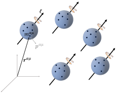
Figure 1: Schematic of our model system. Each molecule with CM at $\mathbf{r}^{\alpha}$ (large blue spheres) is composed of many point-like particles (small black spheres) located at $\mathbf{r}^{\alpha\mu}$ with mass $m^{\alpha\mu}$ and momentum $\mathbf{p}^{\alpha\mu}$. Each molecule has the same angular momentum ${\bm{\ell}}^{\alpha}$, which could be a consequence of e.g. an external field. The angular momentum breaks rotational symmetry.

Odd viscosity, often called gyro viscosity, has been studied for some time in gases Kagan and Maksimov (1967) and plasmas in a magnetic field Braginskii (1958); Landau et al. (1981), and in superfluid He³ Vollhardt and Wolfle (2013). It was first discussed by Avron and co-workers in the context of quantum-Hall fluids Avron et al. (1995) and hypothetical 2D odd fluids Avron (1998) in which OV is compatible with rotational isotropy. Subsequently, the effects of OV in quantum-Hall fluids were thoroughly investigated Hoyos (2014); Read (2009); Read and Rezayi (2011); Bradlyn et al. (2012); Delacrétaz and Gromov (2017). Recent research has paid much less attention to 3D systems.

The fact that TRS is inherently broken in active matter inspired recent investigations of OV in classical active materials Banerjee et al. (2017); Ganeshan and Abanov (2017); Abanov et al. (2018); Lapa and Hughes (2014); Lucas and Surówka (2014); Tsai et al. (2005), all of which focused on 2D fluids. Most of these studied the phenomenology of OV, though Ref. Banerjee et al. (2017) derives the OV from an assumed hydrodynamic action and Ref. Han et al. (2020) presents a semi-microscopic theory for 2D active chiral fluids in which OV is found numerically using Langevin dynamics simulations. Odd viscosity has also been experimentally confirmed in 2D Soni et al. (2019), verifying the existence of unidirectional edge-states Abanov et al. (2018); Souslov et al. (2019).

In this paper we present a first-principles microscopic Hamiltonian theory for odd viscosity in both 2D and 3D using the Poisson-Bracket (PB) approach Hohenberg and Halperin (1977); Stark and Lubensky (2003); Chaikin and Lubensky (1995). Our theory, valid even at zero temperature, suggests that any system with globally or locally aligned spinning components has global (or local) OV arising from kinetic energy alone (other contributions are possible). We discuss some consequences of OV in 3D fluids, including the breakdown of Bernoulli’s principle and the existence of anisotropically propagating bulk transverse velocity waves. We further show that OV should be present in many active matter systems, including 3D ones. Specifically, we expect to find signatures of OV in swimming bacteria and actomyosin networks.

We view a fluid as a large collection of particles (rigid molecules), with center-of-mass (CM) position $\mathbf{r}^{\alpha}$, each composed of multiple sub-particles (atoms) with mass $m^{\alpha\mu}$ and momentum $\mathbf{p}^{\alpha\mu}$ located at $\mathbf{r}^{\alpha\mu}$, Fig. 1. The total momentum density is $\hat{\bf g}(\mathbf{r})=\sum_{\alpha\mu}{\bf p}^{\alpha\mu}\delta\left(\mathbf{r}-\mathbf{r}^{\alpha\mu}\right)$, which, when coarse-grained, becomes Sup ; Martin et al. (1972)

$$\mathbf{g}(\mathbf{r})=\mathbf{g}^{c}+\frac{1}{2}{\bm{\nabla}}\times{\bm{\ell}}\,,$$ (1)

where ${\bf g}^{c}=\rho\mathbf{v}^{c}$ is the CM momentum density, $\rho$ the mass density, $\mathbf{v}^{c}$ the CM velocity, and ${\bm{\ell}}(\mathbf{r})={\underline{\underline{\bm{I}}}}\cdot{\bm{\Omega}}$ is the angular-momentum density of spinning particles, where ${\underline{\underline{\bm{I}}}}$ is the moment-of-inertia density and ${\bm{\Omega}}$ is the rotation-rate vector. Because by definition ${\bm{\ell}}=0$ for point-like particles, we necessarily consider complex particles. Although ${\bm{\ell}}$ affects local momentum both in the bulk and on the surface, it does not contribute to the total momentum because $\int\mathrm{d}\mathbf{r}\,{\bm{\nabla}}\times{\bm{\ell}}=0$. It does, however, contribute to the total angular momentum, ${\bm{L}}=\int\mathrm{d}\mathbf{r}\left(\mathbf{r}\times{\bf g}^{c}+{\bm{\ell}}\right)$. Like a magnetic field, $\bm{\ell}$ is a pseudovector that is even under parity (P) and odd under TR.

Balance of angular momentum implies that the stress tensor ${\bm{\sigma}}$ associated with $\mathbf{g}$ can always be symmetrized Martin et al. (1972). Then, the viscosity $\eta_{ijkl}$ is invariant under the exchanges $i\leftrightarrow j$ and $k\leftrightarrow l$. On the other hand, $\mathbf{g}^{c}$ does not count all momentum, and its stress tensor ${\bm{\sigma}}^{c}$ can have antisymmetric contributions. As shown below, a ‘proper’ OV (obeying ORR) appears in ${\bm{\sigma}}$, while ${\bm{\sigma}}^{c}$ contains only one part of it.

In writing (1) we assume the system is structurally isotropic. However, the presence of ${\bm{\ell}}$ breaks rotational invariance. The essential features of OV are seen for a purely kinetic Hamiltonian, which is written within our model after coarse graining Sup ; Markovich and Lubensky (2021) as .

$$H=\int\mathrm{d}\mathbf{r}\,\frac{\mathbf{g}^{2}}{2\rho}=\int\mathrm{d}\mathbf{r}\left[\frac{(\mathbf{g}^{c})^{2}}{2\rho}+\bm{\ell}\cdot\bm{\omega}^{c}\right]\,,$$ (2)

where ${\bm{\omega}^{c}}=\frac{1}{2}{\bm{\nabla}}\times{\bf v}^{c}$ is half the fluid vorticity and ${\bf g}=\rho{\bf v}$ with $\mathbf{v}$ the fluid velocity. Note that in the second equality we dropped a non-hydrodynamic term $\sim({\bm{\nabla}}\times{\bm{\ell}})^{2}$. Although this Hamiltonian is standard in terms of $\mathbf{g}$, it is peculiar in terms of $\mathbf{g}^{c}$, where the second term couples angular momentum density and vorticity. This term was added ad-hoc (with opposite sign) in Banerjee et al. (2017); Lingam (2015) to a hydrodynamic action and was crucial in deriving the OV.

As detailed in Sup , using the PBs Stark and Lubensky (2005)

$$\{g^{c}_{i}(\mathbf{r}),\rho(\mathbf{r}^{\prime})\} = \rho(\mathbf{r})\nabla_{i}\delta(\mathbf{r}^{\prime}-\mathbf{r})\,,$$

$$\{g_{i}^{c}(\mathbf{r}),g_{j}^{c}(\mathbf{r}^{\prime})\} = g_{i}^{c}(\mathbf{r}^{\prime})\nabla_{j}\delta(\mathbf{r}-\mathbf{r}^{\prime})-\nabla^{\prime}_{i}\!\left[g_{j}^{c}(\mathbf{r}^{\prime})\delta(\mathbf{r}-\mathbf{r}^{\prime})\right],$$

$$\{\ell_{i}(\mathbf{r}),\ell_{j}(\mathbf{r}^{\prime})\} = -\varepsilon_{ijk}\ell_{k}(\mathbf{r})\delta(\mathbf{r}-\mathbf{r}^{\prime})\,,$$

$$\{\ell_{i}(\mathbf{r}),g_{j}^{c}(\mathbf{r}^{\prime})\} = \ell_{i}(\mathbf{r}^{\prime})\nabla_{j}\delta(\mathbf{r}-\mathbf{r}^{\prime})\,,$$ (3)

give the non-dissipative part of the dynamics for the total momentum that satisfies $\dot{g}_{i}+\nabla_{j}\left(v_{j}g_{i}\right)=\nabla_{j}\sigma_{ij}$, where

$$\sigma_{ij}=-P\delta_{ij}+\left(\eta^{e}_{ijkl}+\eta^{o}_{ijkl}\right)\nabla_{l}v_{k}\,,$$ (4)

is the complete stress tensor with $P$ the hydrostatic (thermodynamic) pressure. When anisotropic dissipative terms associated with ${\bm{\ell}}$ are ignored, $\eta^{e}_{ijkl}=\lambda\delta_{ij}\delta_{kl}+\eta\left(\delta_{ik}\delta_{jl}+\delta_{jk}\delta_{il}\right)$, where $\lambda$ and $\eta$ are constants Sup . The odd viscosity,

$$\eta^{o}_{ijkl}=-\frac{1}{4}\ell_{n}\left(\varepsilon_{jln}\delta_{ik}+\varepsilon_{iln}\delta_{jk}+\varepsilon_{ikn}\delta_{jl}+\varepsilon_{jkn}\delta_{il}\right)\,,\quad$$ (5)

naturally emerges from Eqs. (2)-(Odd viscosity in active matter: microscopic origin and 3D effects), revealing its non-dissipative nature. ${\bm{\ell}}$ can be a function of space and time to create “localized” OV . When ${\bm{\ell}}$ is constant we get Onsager’s OV, where ${\bm{\ell}}$ plays the role of magnetic fields in plasmas Braginskii (1958); Landau et al. (1981). The 2D OV Banerjee et al. (2017); Avron (1998) follows from Eq. (5) by writing ${\bm{\ell}}=\ell\hat{z}$ (for a fluid in the $xy$ plane), thereby converting the Levi-Civita tensor to $\varepsilon_{ij}=\varepsilon_{ijz}$. Remarkably, unlike magnetic field in plasmas, this result is purely mechanical and does not require thermodynamic equilibrium or statistical mechanics.

We continue with some phenomenological consequences of OV in 3D. We focus, for simplicity, on the case of constant (in space and time) ${\bm{\ell}}$, which may originate in external driving as described in Sup and Refs. Tsai et al. (2005); Banerjee et al. (2017); van Zuiden et al. (2016)), and experimentally realized in 2D “fluid” metamaterials Tsai et al. (2005); Soni et al. (2019). The ‘odd’ Navier-Stokes equation (NSE), Eq. (4), then reads

$$\dot{g}_{i}+\nabla_{j}\left(v_{j}g_{i}\right) = -\nabla_{i}\tilde{P}+\eta\nabla^{2}v_{i}+\frac{1}{2}{\bm{\ell}}\cdot\nabla\omega_{i}$$ (6)

$$- \frac{1}{2}\varepsilon_{ikn}\ell_{n}\nabla_{k}\nabla\cdot\mathbf{v}\,,$$

with $\tilde{P}\equiv P-(\lambda+\eta)\nabla\cdot\mathbf{v}+{\bm{\ell}}\cdot{\bm{\omega}}$ being the mechanical pressure (diagonal part of the stress) and $\bm{\omega}=\frac{1}{2}{\bm{\nabla}}\times\mathbf{v}$. To investigate the mode structure we linearize Eq. (6) and the continuity equation, $\dot{\rho}+\nabla\cdot(\rho\mathbf{v})=0$, and use Fourier-Transform $\left[{\bf v},\delta\rho\right]=\int\frac{\mathrm{d}\bf k}{(2\pi)^{3}}\left[\tilde{\bf v},\delta\tilde{\rho}\right]\mathrm{e}^{i\left({\bf k}\cdot\mathbf{r}-st\right)}$ to obtain:

$$\begin{pmatrix}s+i\nu k^{2}&-i\tilde{\ell}kk_{\parallel}&2i\tilde{\ell}kk_{\perp}&0\\ i\tilde{\ell}kk_{\parallel}&s+i\nu k^{2}\,\,&0&0\\ -2i\tilde{\ell}kk_{\perp}&0&s+i\nu_{L}k^{2}&-kc\\ 0&0&-kc&s\end{pmatrix}\begin{pmatrix}\tilde{v}_{1}\\ \tilde{v}_{2}\\ \tilde{v}_{L}\\ \tilde{h}\end{pmatrix}=0\,.\quad$$ (7)

Here $\nu\equiv\eta/\rho_{0}$, $\nu_{L}\equiv 2\nu+\lambda/\rho_{0}$, $\tilde{\ell}\equiv\ell/(4\rho_{0})$, ${\bm{\ell}}=\ell\hat{z}$, and $h=\delta\rho/(c\rho_{0})$ where $\rho=\rho_{0}+\delta\rho$ and $c$ is the sound speed ($c^{2}=\partial P/\partial\rho$). We further define $v_{1,2}\equiv\mathbf{v}\cdot\hat{\bf e}_{1,2}$ and $v_{L}\equiv\mathbf{v}\cdot\hat{\bf k}$, where $\hat{\bf k}=(k_{x},k_{y},k_{z})/k$, $\hat{\bf e}_{1}=(-k_{y},k_{x},0)/k_{\perp}$, and $\hat{\bf e}_{2}=(-k_{x}k_{z},-k_{y}k_{z},k_{\perp}^{2})/(kk_{\perp})$ are a set of orthonormal vectors with $k=\sqrt{{\bf k}^{2}}$, $k_{\perp}=\sqrt{k_{x}^{2}+k_{y}^{2}}$, and $k_{\parallel}={\bf k}\cdot{\bm{\ell}}/\ell$.

When dissipation ($\nu$, $\nu_{L}$) is negligible, the matrix in Eq. (7) is Hermitian, with real eigenvalues, and corresponding orthogonal eigenvectors. Hence, there are no instabilities and novel ‘odd’ mechanical waves always propagate. The full solution for the inviscid case can be found in Sup (Eq. (81)). Figure 2 presents a polar plot of the ‘odd’ excitation frequencies $s_{\pm}$ for various $\tilde{\ell}$. We find that $s_{-}$ ($s_{+}$) reaches its maximal value for $\alpha=0$ ($\alpha=45^{\circ}$), where ${\bm{\ell}}\cdot{\bf k}=\cos\alpha$. These modes are always admixture of transverse (T) and longitudinal (L) modes, except when $\alpha=0$, in which case, $s_{+}$ ($s_{-}$) is the L mode for $k\tilde{\ell}<c$ ($k\tilde{\ell}>c$).

The upper left (lower right) $2\times 2$ submatrix of Eq. (7) deals with transverse (longitudinal) variables only, where $2\tilde{\ell}kk_{\perp}$ couples the two. The dimensionless measure of this quantity is $g=2\tilde{\ell}k_{\perp}/c$, which becomes arbitrarily small as $k_{\perp}$ becomes less than $c/(2\tilde{\ell})$. Thus, in the hydrodynamic limit, T and L modes decouple. The frequencies with lowest-order coupling corrections are

$$s_{T} =(\pm\tilde{\ell}kk_{\parallel}-i\nu k^{2})(1-2\tilde{\ell}^{2}k_{\perp}^{2}/c^{2})$$ (8)

$$s_{L} =\pm ck\left(1+2\frac{\tilde{\ell}^{2}k_{\perp}^{2}}{c^{2}}-\frac{1}{8}\frac{\nu_{L}k^{2}}{c^{2}}\right)-\frac{1}{2}i\nu_{L}k^{2}\,,$$ (9)

and the associated eigenvectors [$\vec{v}=(v_{1},v_{2},v_{L},h)$] to lowest order in $g$ and $g_{\nu}=k\nu_{L}/c$ are: $\vec{v}_{L}=(\mp ig,0,1,\pm 1+ig_{\nu}/2)$ and $\vec{v}_{T}=(1,\mp i,0,-ig)$. As expected Avron (1998), the transverse polarizations are purely circular in the $g\rightarrow 0$ limit. When dissipative viscosities are nonzero, the transverse-mode frequency becomes purely diffusive for $k_{\parallel}=0$. A detailed analysis of the general case with arbitrary $\bm{k}$ and the associated phase diagram showing regions with diffusing and propagating modes is deferred to Sup .

It is instructive to see how breaking TRS and parity by ${\bm{\ell}}$ affects normal modes and field couplings. Define the signature of a field to be $({\rm TR},{\rm P})$. $v_{1}$ and $v_{L}$ have signature $(-,+)$, $v_{2}$ $(-,-)$, and $\tilde{\ell}$ $(-,+)$. Thus, $\tilde{\ell}kk_{\parallel}$ with signature $(-,-)$ couples $\dot{v}_{1}$ to $v_{2}$, creating a propagating transverse mode, and $\tilde{\ell}kk_{\perp}$ with signature $(-,+)$ couples $\dot{v}_{1}$ to $v_{L}$, thus mixing longitudinal and transverse components. The transverse $v_{1}-v_{2}$ block in Eq. (7) is similar to the equation for magnons in ferromagnets Kittel (2005) with magnetization ${\mathbf{M}=(M_{x},M_{y},M_{z})}$ with signature $(-,+)$. $M_{x}$ and $M_{y}$ play the role of $v_{1}$ and $v_{2}$, and $M_{z}$ the role of $\tilde{\ell}$. The magnon has an isotropic, rather than an anisotropic, dispersion relation $\omega\propto k^{2}$, reflecting the fact that in the absence of spin-orbit couplings $\mathbf{M}$ rotates under a different group than spatial points.

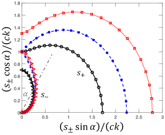
Figure 2: A polar plot of the two normalized ‘odd’ excitations as function of the angle $(\alpha)$ between ${\bm{\ell}}$ and ${\bf k}$. Black lines (reverse triangle for $s_{-}$ and circles for $s_{+}$) are for $k\tilde{\ell}/c=0.7$, blue lines (plus for $s_{-}$ and asterisk for $s_{+}$) are for $k\tilde{\ell}/c=1$, and the red lines (triangles for $s_{-}$ and squares for $s_{+}$) are for $k\tilde{\ell}/c=1.3$. These anisotropic excitations are similar to those found in columnar liquid crystals de Gennes (1980) and nematic elastomers Stenull and Lubensky (2004).

An important and useful simplification of the odd NSE (Eq. (6)) is its incompressible limit, ${\bm{\nabla}}\cdot{\bf v}=0$:

$$\dot{g}_{i}+\nabla_{j}\left(v_{j}g_{i}\right)=-\nabla_{i}\tilde{P}+\eta\nabla^{2}v_{i}+\frac{1}{2}{\bm{\ell}}\cdot\nabla\omega_{i}\,,$$ (10)

where now $\tilde{P}\equiv P+{\bm{\ell}}\cdot{\bm{\omega}}$. Notice that in 2D the last term vanishes, and because $\tilde{P}$ is not a state variable but rather is obtained from the incompressibility constraint, the (bulk) flow is not affected by OV Ganeshan and Abanov (2017). However, this is not the case in 3D, thus one should expect very different phenomenology from that of 2D, even for incompressible fluid.

In order to understand the incompressible limit it is useful to examine the longitudinal equation. The latter is obtained by taking the divergence Eq. (6) and using the continuity equation:

$$\left[\partial_{t}^{2}-\frac{\lambda+2\eta}{\rho_{0}}\nabla^{2}\partial_{t}\right]\delta\rho-\nabla^{2}\left(P+{\bm{\ell}}\cdot{\bm{\omega}}\right)=0\,.$$ (11)

In normal fluids (${\bm{\ell}}=0$), incompressibility is attained by setting $\delta\rho=0$, implying that $\nabla^{2}P=0$. This constraint is not affected by transverse diffusion modes or by local vorticity. In the present case, the constraint $\delta\rho=0$ implies that $\nabla^{2}(P+{\bm{\ell}}\cdot{\bm{\omega}})=0$. But in the presence of a transverse wave, in which ${\bm{\ell}}\cdot{\bm{\omega}}$ is nonzero, $P$ must undergo a compensating change, which normally means that $\delta\rho$ must do so as well. The resolution requires consideration of the limit $c\rightarrow\infty$. The eigenvectors $\vec{v}_{T}$ and $\vec{v}_{L}$ following Eq. (9) reveal that $\delta\rho=-{\bm{\ell}}\cdot{\bm{\omega}}/c^{2}$, which satisfies Eq. (11) for $c\to\infty$ Sup . Because $\delta\rho$ is formally zero, but $\nabla^{2}P$ is not, we could say that a transverse wave produces a (thermodynamic) pressure wave, but not a density wave. Note that although $P$ oscillates, the experimentally accessible $\tilde{P}$ does not. This shows the crucial difference between these two definitions of pressure.

We continue by examining the validity of Bernoulli’s principle in odd fluids. Consider an incompressible, inviscid ($\eta=0$) odd fluid. In steady-state, multiplying Eq. (10) by ${\bf v}$ gives

$$\left({\bf v}\cdot\nabla\right)\left(\frac{\tilde{P}}{\rho}+\frac{1}{2}v^{2}\right)=\frac{1}{2\rho}v_{i}\left({\bm{\ell}}\cdot{\bm{\nabla}}\right)\omega_{i}\,.$$ (12)

As in 2D, the mechanical pressure $\tilde{P}$ takes the place of the thermodynamic pressure $P$. In 2D, the right-hand-side (RHS) of Eq. (12) vanishes and Bernoulli’s principle, in which $\tilde{P}+\frac{1}{2}v^{2}$ is constant along a streamline, is recovered. Furthermore, in 2D the vorticity is conserved along a streamline Acheson (1990), and thus Bernoulli’s principle for $P$ is also restored Avron (1998). In 3D the RHS does not generally vanishes, therefore, Bernoulli’s principle is not valid for ‘odd’ fluids in 3D. Similarly, we observe the breakdown of Kelvin’s circulation theory in 3D odd fluids Sup , and expect to find significant effects on lift and the Magnus effect.

So far we have not discussed the origin of a non-vanishing angular momentum, which requires discussing the dynamics of ${\bm{\ell}}$. The PB approach along with introduction of a torque density ${\bm{\tau}}(\mathbf{r},t)$ , provides the dynamics’ non-dissipative part Sup . Adding a dissipative term $-\Gamma_{ij}(\Omega_{j}-\omega_{j}^{c})$ Markovich et al. (2019b); Stark and Lubensky (2005) that provides preference for a dissipation-free steady-state in which ${\bm{\Omega}}={\bm{\omega}^{c}}$ completes the equation:

$$\dot{\ell}_{i}(\mathbf{r})+\nabla_{j}\left(\ell_{i}v_{j}\right)=\varepsilon_{ijk}\omega_{j}\ell_{k}-\Gamma\left(\Omega_{i}-\omega_{i}\right)+\tau_{i}\,,$$ (13)

where a non-hydrodynamic term $\sim\nabla^{2}{\bm{\ell}}$ was neglected, and we set for simplicity $\Gamma_{ij}=\Gamma\delta_{ij}$. The 2D version of Eq. (13), in which the first term of the RHS vanishes, was first suggested in Tsai et al. (2005) and was used extensively since van Zuiden et al. (2016); Markovich et al. (2019b); Banerjee et al. (2017); De Groot and Mazur (2013). Both TRS and parity are broken by ${\bm{\ell}}$, and the presence of ${\bm{\tau}}$ adds an extra term $\frac{1}{2}\varepsilon_{ijk}\tau_{k}$ to $\sigma_{ij}$ , giving ${\bm{\ell}}$ a non-random value, ${\bm{\ell}}\simeq\underline{\underline{\bf I}}\cdot{\bm{\tau}}/\Gamma$ in the hydrodynamic limit (see Sup Eq. (42)) leading to the appearance of OV, Eq. (5). When ${\bm{\tau}}=0$, $\bm{\Omega}$ relaxes in microscopic times to a function of $\bm{\omega}$, which rapidly vanishes as the fluid approaches equilibrium.

Equation (4) gives the dynamics of $\mathbf{g}$, for which a symmetric stress tensor can always be found (up to $\frac{1}{2}\varepsilon_{ijk}\tau_{k}$ that appears in the presence of body torques). The dynamics of $\mathbf{g}^{c}$ assumes a similar form Sup , $\dot{g}^{c}_{i}+\nabla_{j}\left(v^{c}_{j}g^{c}_{i}\right)=\nabla_{j}\sigma^{c}_{ij}$, but with

$$\sigma^{c}_{ij} = -P\delta_{ij}+\left[\eta^{e}_{ijkl}-\frac{1}{2}\ell_{n}\varepsilon_{jkn}\delta_{il}\right]\nabla_{l}v^{c}_{k}$$ (14)

$$- \frac{1}{2}v^{c}_{i}\left(\nabla\times{\bm{\ell}}\right)_{j}+\frac{\Gamma}{2}\varepsilon_{ijk}\left(\Omega_{k}-\omega^{c}_{k}\right)\,,$$

that has an antisymmetric dissipative part to ensure conservation of angular momentum when $\bm{\tau}=0$, and both symmetric and antisymmetric reactive parts, but only one part of Onsager’s OV (Eq. (5)). This contrasts with current literature Banerjee et al. (2017); Souslov et al. (2019); Han et al. (2020) in which the CM stress tensor ${\bm{\sigma}}^{c}$ is assumed to include both the ‘proper’ OV and the antisymmetric dissipative term .

In Sup we show that after integrating out ${\bm{\Omega}}$, the CM stress tensor has the proper Onsager OV, terms proportional to $\nabla\times{\bm{\ell}}$, and an additional reactive antisymmetric viscosity contribution $\frac{1}{2}\ell_{k}\varepsilon_{ijk}\nabla\cdot\mathbf{v}$. The latter violates ORR and implies that $\dot{\bm{\ell}}\neq 0$ (see Sup ). The corollary is that even after relaxation of ${\bm{\Omega}}$, the CM description cannot properly describe a system with ${\bm{\ell}}\neq 0$, because it does not conform with the balance of angular momentum (an exception is a fluid of constant density).

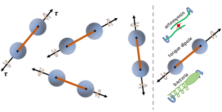
Figure 3: Illustration of a fluid of torque dipoles that shows inhomogeneous OV. On the right - torque dipole as a model for toque exerted by bacteria (where its head and flagellar are rotating in opposite directions) and for a myosin twisting two actin filaments Markovich et al. (2019b).

Although we explore in detail the constant ${\bm{\ell}}$ case, our framework does not restrict $\bm{\ell}$ to be constant in space or time. In fact, in internally driven active materials (such as all natural active materials) the total active torque must vanish Markovich et al. (2019b), implying that ${\bm{\tau}}$ is a divergence of some quantity. For example, in an isotropic active gel (e.g. actomyosin gel) ${\bm{\tau}}=\tilde{\tau}{\bm{\nabla}}\rho$ where $\tilde{\tau}$ is a pseudoscalar (see derivation in Sup Sec. V). Therefore, we expect to have numerous realizations of 3D OV ranging from swimming bacteria Tjhung et al. (2017) and actomyosin networks Markovich et al. (2019b) to swimming microrobots (see Fig. 3).

We have presented a microscopic Hamiltonian theory for the appearance of odd viscosity in active fluids. Being a Hamiltonian theory, no dissipation is required to obtain the OV terms. Our central result is an equation of motion for the total momentum density of non-interacting spinning particles that is valid for arbitrary local values of the angular momentum density ${\bm{\ell}}$.  This equation, which is the analogue of Bloch equations for magnetization, yields the OV predicted by Onsager. Interactions among particles, which we do not consider, modify the OV value but not its form.

Our work considerably extends the applicability of OV into 3D systems and specifically shows its relevance in biological realizations and systems in which torques are generated internally. Examples for such biological realizations range from bacterial suspensions to actomyosin networks, and may even be present in active biopolymer networks without motors Chen et al. (2020) where filaments chirality couples force and twist. It is our hope this work will promote a variety of studies on odd viscosity in 3D systems, from ferronematics to active gels. For instance, it would be interesting to investigate the appearance of odd viscosity in the presence of nematic or polar order.