On the existence of shear-current effects in magnetized burgulence

Abstract

The possibility of explaining shear flow dynamos by a magnetic shear-current (MSC) effect is examined via numerical simulations. Our primary diagnostics is the determination of the turbulent magnetic diffusivity tensor $\boldsymbol{\eta}$. In our setup, a negative sign of its component $\eta_{yx}$ is necessary for coherent dynamo action by the SC effect. To be able to measure turbulent transport coefficients from systems with magnetic background turbulence, we present an extension of the test-field method (TFM) applicable to our setup where the pressure gradient is dropped from the momentum equation: the nonlinear TFM (NLTFM). Our momentum equation is related to Burgers’ equation and the resulting flows are referred to as magnetized burgulence. We use both stochastic kinetic and magnetic forcings to mimic cases without and with simultaneous small-scale dynamo action. When we force only kinetically, negative $\eta_{yx}$ are obtained with exponential growth in both the radial and azimuthal mean magnetic field components. Using magneto-kinetic forcing, the field growth is no longer exponential, while NLTFM yields positive $\eta_{yx}$. By employing an alternative forcing from which wavevectors whose components correspond to the largest scales are removed, the exponential growth is recovered, but the NLTFM results do not change significantly. Analyzing the dynamo excitation conditions for the coherent SC and incoherent $\alpha$ and SC effects shows that the incoherent effects are the main drivers of the dynamo in the majority of cases. We find no evidence for MSC-effect-driven dynamos in our simulations.

1 Introduction

In recent years, there has been a lot of interest in the possibility of large-scale dynamo (LSD) action through the shear-current effect (Rogachevskii & Kleeorin, 2003, 2004) in flows where more conventional dynamo effects, such as the $\alpha$ effect arising through stratification and rotation, cannot operate. In turbulence lacking helicity due to, say, the absence of rotation or stratification in density or turbulence intensity, the $\alpha$ tensor vanishes. The turbulent magnetic diffusivity tensor $\boldsymbol{\eta}$, however, is always found to have finite and positive diagonal components. Its off-diagonal components are in general also finite if there is rotation or shear. Rotation alone gives rise to the $\bm{\Omega}\times\bm{J}$ or Rädler effect (Rädler, 1969a, b) and shear alone to the shear-current (SC) effect. For a suitable sign of the relevant off-diagonal component of $\boldsymbol{\eta}$, the latter effect can lead to dynamo action even without rotation, but the former would not do so without shear. Both the Rädler and SC effects have been discussed as additional or even major dynamo effects in stars (Pipin & Seehafer, 2009), accretion disks (Lesur & Ogilvie, 2008; Blackman, 2010), and galactic magnetism (Chamandy & Singh, 2018).

Astrophysical flows are also subject to vigorous small-scale dynamo (SSD) action, which should occur in any flow where the magnetic Reynolds and Prandtl numbers are large enough. The SSD produces strong, fluctuating magnetic fields at scales smaller than the forcing scale of the turbulence, on time scales short in comparison to the LSD instability (see, e.g., Brandenburg et al., 2012). Usually, the SSD is thought to be detrimental to $\alpha$-effect-driven dynamos, where dynamo action can be strongly suppressed in regimes with high magnetic Reynolds number (e.g., Cattaneo & Vainshtein, 1991; Vainshtein & Cattaneo, 1992), unless the system can get a rid of small-scale magnetic helicity by interacting with its surroundings through helicity fluxes (e.g., Blackman & Field, 2001; Brandenburg, 2001; Brandenburg & Subramanian, 2005). In the absence of magnetic background turbulence it has not yet been possible to verify the existence of a dynamo driven by the SC effect (Brandenburg et al., 2008; Yousef et al., 2008b; Singh & Jingade, 2015). Failure to understand the origin of large-scale magnetic fields in these numerical works in terms of the SC effect, together with the findings of significant $\alpha$ fluctuations in Brandenburg et al. (2008), provided enough motivation to explore the possibility of LSD action driven solely by a fluctuating $\alpha$ in shearing systems. Such an incoherent $\alpha$-shear dynamo was studied analytically in a number of previous works, suggesting a possibility of generation of large-scale magnetic fields due to purely temporal fluctuations in $\alpha$ in the presence of shear (Heinemann et al., 2011; Mitra & Brandenburg, 2012; Sridhar & Singh, 2014).

It has been claimed, however, that in the presence of forcing in the induction equation, mimicking magnetic background turbulence provided, e.g., by the SSD, a thus magnetically driven SC dynamo effect exists (Squire & Bhattacharjee, 2015a, b, 2016). In their analytic study, under the second-order correlation approximation (SOCA), Squire & Bhattacharjee (2015a) argued for a significant magnetic contribution of the type leading to coherent dynamo action in systems with both shear and rotation with typical $q=-S/\Omega$ values for galactic or accretion disks, while in the regime of shear dominating over rotation, relevant to our current study, such contribution was found to be weak. In Squire & Bhattacharjee (2016), it was furthermore argued that the magnetic shear-current (MSC) effect “arises exclusively from the pressure response of the velocity fluctuations.” As we demonstrate in Appendix C, based on an analytical calculation, a magnetic contribution to $\eta_{yx}$ exists even when the pressure term is dropped, but then it likely has a sign that is unfavorable for dynamo action. However, since these analytic results suffer from many simplifications, they cannot provide a conclusive picture. Hence, it is important to study this issue numerically, which is one of our aims in this work.

In their numerical studies, Squire & Bhattacharjee (2015b, 2016) reported the generation of a large-scale magnetic field, usually on the scale of the computational domain, with magnetic forcing, while in the case of kinetic forcing only, the generated patterns were reported to be temporally more erratic and spatially less coherent. For a flow in the $y$ direction, sheared in $x$, an attempt was made to measure the turbulent transport coefficients using the second-order cumulant expansion method of Marston et al. (2008), and the results indicated negative $\eta_{yx}$ and $\eta_{xx}$ in the presence of magnetic forcing (Squire & Bhattacharjee, 2015b). Incidentally, if confirmed in this case, a negative $\eta_{xx}$ could also imply dynamo action (Lanotte et al., 1999; Devlen et al., 2013). At that time, however, a suitable test-field method (TFM), providing another measurement tool for the turbulent transport coefficients, was not yet available.

Here, we present first steps toward such a toolbox, extending the method developed by Rheinhardt & Brandenburg (2010, hereafter RB10) to include the self-advection term and rotation, albeit still limited to simplified MHD (SMHD) equations, with the pressure gradient term being dropped. Although this method does not yet provide a completely suitable tool for the systems studied by Squire & Bhattacharjee (2015b, 2016), it does provide a working solution for simplified shear dynamos with magnetic forcing, mimicking SSD, and can be envisioned to enable important scientific insights. In this paper, we present the method, referred to as the “nonlinear test-field method” (NLTFM), and tests against previously studied cases, along with other validation results. As our major topic, we analyze runs with SMHD equations that exhibit dynamo action in the same parameter regime as previously claimed to host MSC-effect dynamos.

2 Model and Methods

We perform local Cartesian box simulations with shearing-periodic boundary conditions to implement large-scale shear as a linear background flow imposed on the system. The shear occurs in the $x$ direction, which could represent, e.g., the direction from the rotational center of a cosmic body. Here, $y$ is the streamwise, or azimuthal, direction, and $z$ points into the vertical direction. The magnitude of the shearing motion is described by the input parameter $S$ such that the imposed linear shear flow is ${\bm{U}}^{\rm S}=Sx\bm{\hat{y}}.$ The rotation of the domain, ${\bm{\Omega}}=(0,0,\Omega)$, is described by the input parameter $\Omega$, the magnitude of the angular velocity. In the simulations reported in this paper, however, rotation is neglected, as here we concentrate on studying the possibility of the SC effect alone. We will, however, retain rotation in the model equations for completeness. Our boxes have edge lengths $L_{x}=L_{y}$, and $L_{z}$ with aspect ratio ${\cal A}=L_{z}/L_{x}$ chosen equal to one in many cases, but we consider also vertically elongated boxes with ${\cal A}=4,8,16$. All calculations were carried out with the Pencil Code, see e.g. Brandenburg et al. (2020).

2.1 Simplified MHD

As stated in the introduction, the equations of SMHD as defined here are similar to those of MHD, but lack the pressure gradient. Correspondingly, the density $\rho$ is held constant. We solve the equations for the magnetic vector potential $\bm{A}$ and the velocity $\bm{U}$,

$${\cal D}{}^{A}\bm{A} = \bm{U}\times\bm{B}+\bm{F}_{\rm M}+\eta{\bm{\nabla}}^{2}\bm{A},$$ (1)

$${\cal D}{}^{U}\bm{U} = -\bm{U}\cdot{\bm{\nabla}}\bm{U}+\bm{J}\times\bm{B}/\rho+\bm{F}_{\rm K}$$ (2)

$$+\nu({\bm{\nabla}}^{2}\bm{U}+{\bm{\nabla}}{\bm{\nabla}}\cdot\bm{U}/3)$$

with the linear expressions

$${\cal D}{}^{A}\bm{A} = {\cal D}{}\bm{A}+SA_{y}\hat{\mbox{\boldmath$x$}}{},$$ (3)

$${\cal D}{}^{U}\bm{U} = ({\cal D}{}+2\bm{\Omega}\times)\bm{U}+SU_{x}\hat{\mbox{\boldmath$y$}}{},$$ (4)

$$\cal D = \partial_{t}+Sx\partial_{y}.$$ (5)

$\bm{B}={\bm{\nabla}}\times\bm{A}$ is the magnetic field, $\bm{J}={\bm{\nabla}}\times\bm{B}$ is the current density in units where the vacuum permeability is unity, $\bm{F}_{\rm K}$ and $\bm{F}_{\rm M}$ are kinetic and magnetic forcing functions, respectively, $\eta$ is the (molecular) magnetic diffusivity, and $\nu$ is the kinematic viscosity, both assumed constant. Equation (2) can be considered a three-dimensional generalization of Burgers’ equation, which is why one refers to its turbulent solutions as “burgulence”; see the review by Frisch & Bec (2001) on such flows.

The main advantage of using SMHD is to avoid the necessity of dealing with density fluctuations and corresponding effects in the mean quantities. However, as self-advection $\bm{U}\cdot{\bm{\nabla}}\bm{U}$ is no longer discarded, we are here more general than RB10, the models of which suffered, in physical terms, from the implied assumption of slow fluid motions, that is, small Strouhal numbers ($\mbox{\rm St}\ll 1$) or Reynolds numbers ($\mbox{\rm Re}\ll 1$). Completely neglecting the self-advection term is inadequate in the present context given that shear plays its essential role just via this term. So merely the terms arising from an additional mean flow and from the fluctuating velocity alone could be dropped. Neglecting the latter, however, would be equivalent to restricting the method to SOCA with respect to the self-advection term, which is not desirable.

2.2 Full MHD

The full MHD (FMHD) system of equations, here with an isothermal equation of state, is more complex because of the occurrence of the pressure gradient, as a result of which we need an additional evolution equation for the density. Also the viscous force is more complex, hence

$${\cal D}{}^{A}\bm{A} = \bm{U}\times\bm{B}+\bm{F}_{\rm M}+\eta{\bm{\nabla}}^{2}\bm{A},$$

$$\rho({\cal D}{}^{U}+\bm{U}\cdot{\bm{\nabla}})\bm{U}+{\bm{\nabla}}p = \bm{J}\times\bm{B}+\rho\bm{F}_{\rm K}+{\bm{\nabla}}\cdot(2\nu\rho\mbox{\boldmath${\sf S}$}{}),$$

$$({\cal D}{}+\bm{U}\cdot{\bm{\nabla}})\ln\rho = -{\bm{\nabla}}\cdot\bm{U}.$$ (6)

Here, ${\sf S}_{ij}=(U_{i,j}+U_{j,i})/2-\delta_{ij}{\bm{\nabla}}\cdot\bm{U}/3$ are the components of the rate-of-strain tensor ${\sf S}$, where commas denote partial differentiation, and $p$ is the pressure related to the density via $p=c_{\rm s}^{2}\rho$, with $c_{\rm s}={\rm const}{}$ being the isothermal sound speed.

2.3 Test-field methods

Throughout, we define mean quantities by horizontal averaging, i.e., averaging over $x$ and $y$, denoted by an overbar. So the means depend on $z$ and $t$ only. Fluctuations are denoted by lowercase symbols or a prime, e.g., $\bm{a}=\bm{A}-{\overline{\bm{A}}}$, $\bm{u}=\bm{U}-\overline{\bm{U}}$, $(\bm{u}\times\bm{b})^{\prime}=\bm{u}\times\bm{b}-\overline{\bm{u}\times\bm{b}}$, and $\bm{f}_{\rm K,M}=\bm{F}_{\rm K,M}-\overline{\bm{F}}_{\rm K,M}$. The horizontal average is normally taken to obey the Reynolds rules. In situations with linear overall shear though, the complication arises that $\bm{U}^{S}\neq\overline{\bm{U}^{S}}$ (when $\bm{U}^{S}$ is defined to be $\propto x$, the mean even vanishes), being hence not a pure mean, while ${\partial_{i}U^{S}_{j}}$ is spatially constant, hence a pure mean. So the Reynolds rule “averaging commutes with differentiating” is violated. However, $(\bm{U}^{S}\cdot{\bm{\nabla}}G)^{\prime}=\bm{U}^{S}\cdot{\bm{\nabla}}g$ for an arbitrary quantity $G=\overline{G}+g$. This is a consequence of $\bm{U}^{S}\cdot{\bm{\nabla}}\overline{G}=0$ and $\overline{\bm{U}^{S}\cdot{\bm{\nabla}}g}=\int\!\int Sx\,\partial_{y}g\,dxdy=\int Sx\left(\int\partial_{y}g\,dy\right)dx=0$, the latter because of periodicity in $y$. Thus, $\bm{U}^{S}$ can effectively be treated as a mean flow.

The evolution equations for the fluctuations of the magnetic vector potential, $\bm{a}$, and the velocity, $\bm{u}$, follow from Eqs. (1) and (2) as

$${\cal D}{}^{A}\bm{a} = \bm{u}\times{\overline{\bm{B}}}+\overline{\bm{U}}\times\bm{b}+(\bm{u}\times\bm{b})^{\prime}+\bm{f}_{\rm M}+\eta{\bm{\nabla}}^{2}\bm{a},$$ (7)

$${\cal D}{}^{U}\bm{u} = \left(\,{\overline{\bm{J}}}\times\bm{b}+\bm{j}\times{\overline{\bm{B}}}+(\bm{j}\times\bm{b})^{\prime}\right)/\rho$$

$$-(\bm{u}\cdot{\bm{\nabla}}\bm{u})^{\prime}-\overline{\bm{U}}\cdot{\bm{\nabla}}\bm{u}-\bm{u}\cdot{\bm{\nabla}}\overline{\bm{U}}$$

$$+\bm{f}_{\rm K}+\nu\!\left({\bm{\nabla}}^{2}\bm{u}+{\bm{\nabla}}{\bm{\nabla}}\cdot\bm{u}/3\right).$$

2.3.1 Nonlinear TFM

In the quasi-kinematic test-field method (qktfm) (see Sect. 2.3.2), the mean electromotive force $\overline{\mbox{\boldmath${\cal E}$}}{}=\overline{\bm{u}\times\bm{b}}$ is a functional of only $\bm{u}$, $\overline{\bm{U}}$, and ${\overline{\bm{B}}}$ (linear in ${\overline{\bm{B}}}$). However, in the more general case with a magnetic background turbulence, this is no longer so. To deal with this difficulty, RB10 added the evolution equations for the background turbulence ($\bm{u}_{0}$,$\bm{b}_{0}$) which are similar to Eqs. (7) and (2.3), but for zero mean field, to the equations of the TFM. In general, $\overline{\mbox{\boldmath${\cal E}$}}{}=\overline{\bm{u}\times\bm{b}}$ can be split into a contribution $\overline{\mbox{\boldmath${\cal E}$}}{}_{0}=\overline{\bm{u}_{0}\times\bm{b}_{0}}$ that is independent of the mean field and

$$\overline{\mbox{\boldmath${\cal E}$}}{}_{\bm{\bar{B}}}=\overline{\bm{u}_{0}\times\bm{b}_{\bm{\bar{B}}}}+\overline{\bm{u}_{\bm{\bar{B}}}\times\bm{b}_{0}}+\overline{\bm{u}_{\bm{\bar{B}}}\times\bm{b}_{\bm{\bar{B}}}},$$ (9)

where $\bm{u}_{\bm{\bar{B}}}$ and $\bm{b}_{\bm{\bar{B}}}$ denote the solutions of Eqs. (7) and (2.3) without forcing (called “test problems”) which are supposed to vanish for vanishing ${\overline{\bm{B}}}$. Thus, $\bm{u}=\bm{u}_{0}+\bm{u}_{\bm{\bar{B}}}$, $\bm{b}=\bm{b}_{0}+\bm{b}_{\bm{\bar{B}}}$. $\overline{\mbox{\boldmath${\cal E}$}}{}_{\bm{\bar{B}}}$ can be written in two equivalent ways as

$$\overline{\mbox{\boldmath${\cal E}$}}{}_{\bm{\bar{B}}}=\overline{\bm{u}\times\bm{b}_{\bm{\bar{B}}}}+\overline{\bm{u}_{\bm{\bar{B}}}\times\bm{b}_{0}}=\overline{\bm{u}_{0}\times\bm{b}_{\bm{\bar{B}}}}+\overline{\bm{u}_{\bm{\bar{B}}}\times\bm{b}}.$$ (10)

Both become linear in quantities with subscript ${\overline{\bm{B}}}$ when $\bm{b}$ and $\bm{u}$ are identified with the fluctuating fields in the “main run”, which is the system (1)–(2) solved simultaneously with the test problems. In this way, we have recovered the mentioned linearity property of $\overline{\mbox{\boldmath${\cal E}$}}{}[{\overline{\bm{B}}}]$ of the qktfm. Likewise, one writes that part of the mean ponderomotive force $\overline{\mbox{\boldmath${\cal F}$}}{}_{\bm{\bar{B}}}$, which results from the Lorentz force as

$$\overline{\bm{j}\times\bm{b}_{\bm{\bar{B}}}}+\overline{\bm{j}_{\bm{\bar{B}}}\times\bm{b}_{0}}\quad\text{or}\quad\overline{\bm{j}_{0}\times\bm{b}_{\bm{\bar{B}}}}+\overline{\bm{j}_{\bm{\bar{B}}}\times\bm{b}}$$ (11)

and that resulting from self-advection as

$$-\overline{\bm{u}\cdot{\bm{\nabla}}\bm{u}_{\bm{\bar{B}}}}-\overline{\bm{u}_{\bm{\bar{B}}}\cdot{\bm{\nabla}}\bm{u}_{0}}\quad\text{or}\quad-\overline{\bm{u}_{0}\cdot{\bm{\nabla}}\bm{u}_{\bm{\bar{B}}}}-\overline{\bm{u}_{\bm{\bar{B}}}\cdot{\bm{\nabla}}\bm{u}}\,;$$ (12)

see  Eqs. (29) and (30) of RB10. Corresponding expressions can be established for the fluctuating parts of the bilinear terms, $(\bm{u}\times\bm{b})^{\prime}$, $(\bm{j}\times\bm{b})^{\prime}$, and $(\bm{u}\cdot{\bm{\nabla}}\bm{u})^{\prime}$, occurring in Eqs. (7) and (2.3). We recall that these different formulations result in different stability properties of the test problems; see also the test results presented in Appendix B.1. Here, we chose to use in Eqs. (10)–(12), and in the aforementioned expressions for the fluctuating parts of the bilinear terms, the respective first version, that is, $\overline{\mbox{\boldmath${\cal E}$}}{}_{\bm{\bar{B}}}=\overline{\bm{u}\times\bm{b}_{\bm{\bar{B}}}}+\overline{\bm{u}_{\bm{\bar{B}}}\times\bm{b}_{0}}$, $(\bm{u}\times\bm{b})^{\prime}=(\bm{u}\times\bm{b}_{\bm{\bar{B}}})^{\prime}+(\bm{u}_{\bm{\bar{B}}}\times\bm{b}_{0})^{\prime}$ etc. This choice forms what is called the ju method; see Table 1 of RB10.

The given alternative formulations become equivalent when the mean quantities, possibly evolving in the main run, are too weak to have a marked influence on the fluctuating fields. Then, $\bm{u}\rightarrow\bm{u}_{0}$ and $\bm{b}\rightarrow\bm{b}_{0}$, which defines the kinematic limit. Employing this means dropping terms like $\overline{\bm{u}_{\bm{\bar{B}}}\times\bm{b}_{\bm{\bar{B}}}}$ in mean EMF and mean force, which is the correct way to obtain the latter as quantities of first order in ${\overline{\bm{B}}}$. Then all possible versions of the NLTFM (which actually ceases to be nonlinear) give identical results up to roundoff errors.

We solve Eqs. (7) and (2.3) not by setting ${\overline{\bm{B}}}$ to the actual mean field resulting from the solutions of Eqs. (1) and (2), but by setting it to one of four test fields, $\bm{B}^{\rm T}$. Those are

$$\bm{B}^{(1)}=(\cos k_{B}z,0,0),\quad \bm{B}^{(2)}=(\sin k_{B}z,0,0),$$ (13)

$$\bm{B}^{(3)}=(0,\cos k_{B}z,0),\quad \bm{B}^{(4)}=(0,\sin k_{B}z,0),$$ (14)

where $k_{B}$ is the wavenumber of the test field, being a multiple of $2\pi/L_{z}$. From the solutions of Eqs. (7) and (2.3) we can construct the mean electromotive force, $\overline{\mbox{\boldmath${\cal E}$}}{}=\overline{\bm{u}\times\bm{b}}$ and the mean ponderomotive force, $\overline{\mbox{\boldmath${\cal F}$}}{}=\overline{\bm{j}\times\bm{b}/\rho-\bm{u}\cdot{\bm{\nabla}}\bm{u}}$, which are then expressed in terms of the mean field by the ansatzes

$$\overline{\cal E}{}_{i}=\alpha_{ij}\overline{B}_{j}-\eta_{ij}\overline{J}_{j},$$ (15)

$$\overline{\cal F}_{i}=\phi_{ij}\overline{B}_{j}-\psi_{ij}\overline{J}_{j},$$ (16)

where $i,j$ adopt only the values $1,2$ as a consequence of setting $\overline{B}_{z}$, which is constant anyway, arbitrarily to zero. Hence, each of the four tensors, $\alpha_{ij}$, $\eta_{ij}$, $\phi_{ij}$, $\psi_{ij}$, has four components, i.e., altogether we have 16 unknowns. Note that often the $\alpha$ and $\eta$ tensors are defined as just the symmetric parts of our $\alpha_{ij}$ and $\eta_{ij}$ while their antisymmetric parts are cast into the vectorial coefficients of the $\gamma$ and $\delta$ effects. The coefficients $\boldsymbol{\alpha}$, $\boldsymbol{\beta}$, $\boldsymbol{\gamma}$, and $\boldsymbol{\delta}$ describe in turn the effects of turbulent generation, diffusion, pumping and the (non-generative, non-dissipative) so-called Rädler effect. In the presence of shear, the coefficient $\eta_{yx}$ plays a prominent role; see Sect. 3.3. In spite of what could be expected from the Lorentz force, being quadratic in $\bm{B}$, the turbulent ponderomotive force Eq. (16) is linear in ${\overline{\bm{B}}}$. This is because of the presence of the magnetic background turbulence $\bm{b}_{0}$ via, in the kinematic limit, $\overline{\bm{j}_{0}\times\bm{b}_{\bm{\bar{B}}}+\bm{j}_{\bm{\bar{B}}}\times\bm{b}_{0}}$.

2.3.2 Quasikinematic TFM

We state here for comparison the governing equations for the qktfm (see also Schrinner et al., 2005, 2007). They consist of just Eq. (7) with $\bm{f}_{\rm M}=\bm{0}$, but not Eq. (2.3), and Eq. (15). Then, Eq. (10) reduces simply to

$$\overline{\mbox{\boldmath${\cal E}$}}{}_{\bm{\bar{B}}}=\overline{\bm{u}\times\bm{b}_{\bm{\bar{B}}}},$$ (17)

and we find the contribution $\overline{\bm{u}_{\bm{\bar{B}}}\times\bm{b}_{0}}$ missing. Again, for further details see RB10.

2.3.3 Resetting

The test problems Eqs. (7) and (2.3) are often unstable, but this does not necessarily affect the values of the resulting turbulent transport coefficients: They usually show statistically stationary behavior over limited time spans although the test solutions are already growing. For safety reasons, we always reset them to zero in regular intervals (typically every 0.5 viscous times); see Hubbard et al. (2009) for a discussion. To mask the initial transient, we also remove 20% of the data from the beginning of each resetting interval.

2.4 Forcing

The standard forcing, implemented in the Pencil Code, employs white-in-time “frozen” harmonic plane waves, here restricted to be non-helical. Their wavevectors are randomly selected from a thin shell in $k$ space of radius $k_{\rm f}$ such that they fit into the periodic computational domain (for details see, e.g. Käpylä et al., 2020). In most of our simulations, we apply this recipe for both kinetic and magnetic forcings in Equations (1), (1), (7), and (2.3). The wavevectors are further selected such that no mean field or mean flow is directly sustained, that is, the case $k_{y}=0$ is excluded. However, due to roundoff errors, it is unavoidable that averages over harmonic functions deviate slightly from zero. We call this effect “leakage of the forcing into the mean fields”. Strong shear could produce a linearly growing $\overline{B}_{y}$ out of a small $\overline{B}_{x}$ due to such leakage. This is why we checked its effect in purely magnetic runs and found the growth of $\overline{B}_{y}$ to be limited and both components to stay within margins close to numerical precision. Nevertheless, as will be discussed in Sect. 3.1, with this magnetic forcing setup, the mean magnetic fields very quickly (in a few turnover times) reach dynamically effective strengths without showing a clear exponential stage.

Hence, another forcing setup was designed, referred to as “decimated forcing”. In addition to ensuring that $k_{y}=0$ is excluded, we took out all those wavevectors for which $|k_{x,y,z}|\leq k_{\rm min}=2k_{1}$. As will be discussed in the results section, the decimated forcing has the advantage of reducing the amplitude of the mean fields generated during the initial stages, thus allowing us to determine the growth rate of an exponentially growing dynamo instability. While the standard choice is expected to provide a good approximation to homogeneous isotropic velocity turbulence, isotropy could be lost in the decimated case, given that all wavevectors are parallel or almost parallel to the spatial diagonals of the box.

However, as is discussed in Appendix A, the generated turbulence does not markedly deviate from that by the standard forcing in terms of isotropy. Also, repeating the kinetically forced runs ($\bm{f}_{\rm M}=\bm{F}_{\rm M}=\bm{0}$) with decimated forcing does not significantly alter the dynamo solutions.

2.5 Mean flow removal

In every case, be it full or simplified MHD, the first instability to be excited is the generation of a mean flow with horizontal components. These are most likely signatures of the vorticity dynamo (see, e.g., Elperin et al., 2003; Käpylä et al., 2009). As it can destabilize the test problems, we have decided to suppress the mean flow by subtracting it from the solution $\bm{U}$ in every time step, which also avoids leakage of the forcing into $\overline{\bm{U}}$. With respect to a possible effect on the magnetic field, we refer to Yousef et al. (2008a), who reported, for a very similar simulation setup to that used here, that the presence of $\overline{\bm{U}}$ did not significantly change the properties of the shear dynamo; see their Section 3.4.

2.6 Input and output quantities

The simulations are fully defined by choosing the shear parameter $S$, the forcing setup, amplitude, and wavenumber, $k_{\rm f}$, the kinematic viscosity $\nu$, and the magnetic diffusivity $\eta$. For normalizations we use the horizontal length scale $k_{1}^{-1}$, with $k_{1}=2\pi/L_{x}$, which is connected to the vertical length scale $k_{1z}^{-1}={\cal A}/k_{1}$, and the viscous time scale $T_{\nu}=(\nu k_{1}^{2})^{-1}$. The boundary conditions are (shearing) periodic in all three directions. The following quantities are used as diagnostics. We quantify the strength of the turbulence by the fluid and magnetic Reynolds numbers

$$\mbox{\rm Re}=\frac{u_{\rm rms}}{\nu k_{\rm f}},\ \ \ \mbox{\rm Re}_{\rm M}=\frac{u_{\rm rms}}{\eta k_{\rm f}}=\mbox{\rm Pr}_{\rm M}\,\mbox{\rm Re},$$ (18)

where

$$\mbox{\rm Pr}_{\rm M}=\frac{\nu}{\eta},$$ (19)

is the magnetic Prandtl number. The Lundquist number and its ratio to $\mbox{\rm Re}_{\rm M}$ are given by

$$\mbox{\rm Lu}=\frac{B_{\rm rms}}{\eta k_{\rm f}\sqrt{\rho}},\quad\frac{\mbox{\rm Lu}}{\mbox{\rm Re}_{\rm M}}=\frac{B_{\rm rms}}{u_{\rm rms}\sqrt{\rho}},$$ (20)

which is only used in SMHD, where $\rho={\rm const}{}$. The strength of the imposed shear is measured by the dynamic shear number

$$\mbox{\rm Sh}_{\rm K}=\frac{S}{u_{\rm rms}k_{\rm f}}.$$ (21)

As in earlier work, we normalize the turbulent magnetic diffusivity tensor by the SOCA estimate

$$\eta_{0}=u_{\rm rms}/3k_{\rm f}$$ (22)

or the molecular diffusivity $\eta$.

We define the root-mean-square (rms) value of the magnetic field as $B_{\rm rms}=\langle{\bm{B}}^{2}\rangle^{1/2}$ while $\overline{B}_{i,{\rm rms}}=\big{\langle}\overline{B}_{i}^{2}\big{\rangle}_{z}^{1/2}$ are the rms values of the mean field components. $\langle.\rangle$ denotes volume averaging and $\langle.\rangle_{\xi}$ averaging over a coordinate $\xi$. The magnetic field is normalized by the equipartition field strength, $B_{\rm eq}=\langle\langle\rho\bm{u}^{2}\rangle^{1/2}\rangle_{t}$. For the velocity field, we define a time-averaged rms value $u_{\rm rms}=\langle\langle{\bm{u}}^{2}\rangle^{1/2}\rangle_{t}$. Kinematic dynamo growth rates $\lambda$ are defined as $\langle d_{t}\log B_{\rm rms}\rangle_{t}$ or $\langle d_{t}\log\overline{B}_{i,{\rm rms}}\rangle_{t}$.

Table 1: Summary of the runs with constant shear and forcing wavenumber.

Run	$\mbox{\rm Re}_{\rm M}$	$\lambda/(\eta_{0}k_{\rm f}^{2})$	$\eta_{xx}/\eta_{0}$	$\eta_{yy}/\eta_{0}$	$\eta_{yx}/\eta_{0}$aaa	$\eta_{xy}/\eta_{0}$aaa	$\alpha_{\rm rms}/\eta_{0}k_{\rm f}$	$\eta_{\rm rms}/\eta_{0}$
FK1a	2.1	$-$0.0354	0.557$\pm$0.006	0.547$\pm$0.007	0.048$\pm$0.001	0.351$\pm$0.009	0.018$\pm$0.009	0.054$\pm$0.013
FK1b	11.9	0.0140	0.608$\pm$0.015	0.598$\pm$0.014	0.023$\pm$0.001	0.419$\pm$0.032	0.022$\pm$0.011	0.031$\pm$0.012
FK8a	2.1	$-$0.0008	0.572$\pm$0.010	0.563$\pm$0.011	0.044$\pm$0.002	0.378$\pm$0.009	0.001$\pm$0.002	0.048$\pm$0.014
FK8b	12.7	0.0166	0.641$\pm$0.019	0.634$\pm$0.017	0.023$\pm$0.001	0.473$\pm$0.024	0.009$\pm$0.005	0.026$\pm$0.009
SK1a	2.0	0.0006	0.367$\pm$0.001	0.393$\pm$0.002	$-$0.003$\pm$0.000	0.279$\pm$0.002	0.021$\pm$0.004	0.009$\pm$0.001
SK1b	12.3	0.0183	0.440$\pm$0.004	0.412$\pm$0.001	$-$0.011$\pm$0.002	0.461$\pm$0.009	0.020$\pm$0.009	0.017$\pm$0.009
SK4a	2.1	$-$0.0042	0.367$\pm$0.003	0.390$\pm$0.003	$-$0.004$\pm$0.000	0.279$\pm$0.003	0.008$\pm$0.002	0.006$\pm$0.001
SK4b	13.3	0.0185	0.334$\pm$0.037	0.339$\pm$0.044	$-$0.004$\pm$0.005	0.239$\pm$0.073	0.008$\pm$0.004	0.007$\pm$0.008
SK8a	2.1	0.0033	0.367$\pm$0.003	0.390$\pm$0.004	$-$0.003$\pm$0.000	0.274$\pm$0.003	0.006$\pm$0.002	0.005$\pm$0.002
SK8b	12.8	0.0192	0.401$\pm$0.005	0.424$\pm$0.005	$-$0.015$\pm$0.000	0.367$\pm$0.010	0.007$\pm$0.002	0.017$\pm$0.004
SKM1a	1.9	—aa	1.794$\pm$0.039	1.278$\pm$0.045	0.200$\pm$0.025	$-$0.725$\pm$0.083	0.010$\pm$0.055	0.250$\pm$0.090
SKM4a	2.1	—aa	2.012$\pm$0.179	1.191$\pm$0.014	0.221$\pm$0.012	$-$0.560$\pm$0.015	0.046$\pm$0.017	0.230$\pm$0.072
SKM8a	1.8	—aa	3.054$\pm$0.625	1.481$\pm$0.131	0.338$\pm$0.064	$-$0.186$\pm$0.045	0.036$\pm$0.011	0.352$\pm$0.213
SKM16a	2.0	—aa	2.238$\pm$0.552	1.215$\pm$0.010	0.249$\pm$0.062	$-$0.580$\pm$0.055	0.022$\pm$0.008	0.260$\pm$0.191
SKM1ad	2.1	0.0103	1.228$\pm$0.214	1.326$\pm$0.074	0.247$\pm$0.043	0.237$\pm$0.117	0.149$\pm$0.062	0.441$\pm$0.212
SKM4ad	1.9	0.0315	1.279$\pm$0.150	1.455$\pm$0.066	0.222$\pm$0.022	0.369$\pm$0.072	0.081$\pm$0.017	0.270$\pm$0.119
SKM8ad	1.5	0.0948	1.688$\pm$0.165	2.040$\pm$0.150	0.516$\pm$0.061	0.383$\pm$0.154	0.111$\pm$0.069	0.543$\pm$0.260
SKM16ad	1.9	0.0344	1.231$\pm$0.070	1.589$\pm$0.019	0.364$\pm$0.116	0.279$\pm$0.026	0.033$\pm$0.015	0.292$\pm$0.015

Note: For all runs, $k_{\rm f}/k_{1}=5$ and $S=-25/T_{\nu}$ yielding a roughly invariable $\mbox{\rm Sh}_{\rm K}$ of $-1.6$. In runs with labels “a”, the magnetic Prandtl number $\mbox{\rm Pr}_{\rm M}$ is $10/3$, while for “b” it is 20. The integer in the run name indicates the aspect ratio ${\cal A}$ and the letter “d” at the end refers to “decimated forcing”. The number of grid points in the ${\cal A}=1$ models was $144^{3}$, while the number of grid points in the vertical ($z$) direction was increased as ${\cal A}$ increased, so that 288, 576, and 1152 grid points in $z$ were used for ${\cal A}=$4,8, and 16, respectively. The Mach number in the simulations was around 0.03 and 0.04 for low and high $\mbox{\rm Re}_{\rm M}$ runs, respectively. Due to the low $\mbox{\rm Re}_{\rm M}$ in all the models investigated, no small-scale dynamo could get excited, because for flows with low Mach number the critical $\mbox{\rm Re}_{\rm M}$ for this instability is around 30 (see, e.g., Haugen et al., 2004).

3 Results

The naming of the runs is such that the first letter, F or S, indicates full or simplified MHD, while the second and third refer to the forcing regime: K and KM referring to purely kinetic and combined kinetic and magnetic forcing (henceforth magneto-kinetic) with amplitudes equal up to a factor of $\rho^{-1/2}$ in the magnetic force, respectively. The number following the letters indicates the vertical aspect ratio ${\cal A}$ of the box. A trailing letter “d” stands for “decimated forcing”. In FMHD, the sound speed was set to $100/k_{1}T_{\nu}$.

3.1 Overall behavior of the main runs

As our starting point, we defined a setup, related to one from Squire & Bhattacharjee (2015b), with marginal dynamo excitation (in incompressible MHD) and an aspect ratio ${\cal A}=8$. We denote this run as FK8a, and tabulate $\mbox{\rm Re}_{\rm M}$, the growth rate of the initial kinematic stage, $\lambda$, and the $\bm{\eta}$ components measured by QKTFM in Table LABEL:models. As reported by Squire & Bhattacharjee (2015b), we also observe an initial decay of the rms and mean magnetic fields, but later we find temporary saturation at very low values, after which a very slow decay is observed, indicative of a nearly marginally excited dynamo state. Because of the finite $\overline{B}_{x}$ present at all times, a much stronger (roughly 40 times) $\overline{B}_{y}$ is maintained due to the shear, but as the dynamo is nearly marginal, these mean fields remain at very low strengths. We note that most of the magnetic energy is in the mean fields, while only a small fraction (less than 20%) is in the fluctuations.

Next, we repeat this run, but with SMHD, which yields Run SK8a in Table LABEL:models. Now rms and mean fields grow, the mean radial and azimuthal components showing exponential growth at the same rate, albeit still very slow. Nevertheless, the dynamo instability is somewhat easier to excite than in FMHD. The azimuthal component is again much stronger than the radial one with the ratio $\overline{B}_{y,{\rm rms}}$/$\overline{B}_{x,{\rm rms}}$ similar to the FMHD case.

We continue by repeating these runs with decreased magnetic diffusivity, resulting in roughly six times larger magnetic Reynolds number, $\mbox{\rm Re}_{\rm M}$ (Runs FK8b and SK8b). In both simulations we observe exponential growth of the rms and mean magnetic fields, somewhat faster with SMHD than with FMHD. The ratio of the mean field energy to the energy in the fluctuations remains unchanged with respect to the lower $\mbox{\rm Re}_{\rm M}$ (and $\mbox{\rm Pr}_{\rm M}$) runs. We also determine the fastest growing dynamo mode and its vertical wavenumber $k_{z}$ and list them in Table LABEL:dynamonumbers; the fastest growing mode is nearly the same with $k_{z}/k_{1z}=9$ in both models. Hence, we can conclude that going from FMHD to SMHD retains the dynamo mode, but changes its excitation condition and growth rate somewhat.

As the dynamo growth is slow, simulations with ${\cal A}=8$ are too costly to be run until saturation. Hence, to investigate whether with reduced ${\cal A}$ the dynamo mode could be retained, we repeated the runs with ${\cal A}=1$ (Runs FK1a, FK1b, SK1a, and SK1b). As is evident from Tables LABEL:models and LABEL:dynamonumbers, these runs behave very much like their tall-box counterparts, the low-$\mbox{\rm Re}_{\rm M}$ FMHD model being slightly subcritical and the high-$\mbox{\rm Re}_{\rm M}$ one supercritical, while the SMHD runs are both supercritical. The fastest growing mode now has $k_{z}/k_{1}=1$ corresponding to $k_{z}/k_{1z}=8$ in the tall box. We also perform a set of runs in SMHD with ${\cal A}=4$; see Runs SK4a and SK4b. The former exhibits a very slowly decaying solution instead of a growing one, which is an anomaly in the SMHD set, but the latter one again exhibits a growth rate very similar to the cubic (SK1b) and tall-box (SK8b) cases, both with a wavenumber $k_{z}/k_{1z}=4$. All in all, the “b” runs give rather clear evidence that the cubic simulation domains retain the same dynamo mode as the taller ones.

The time evolution of the rms and mean fields from the cubic runs, integrated until saturation, is shown in the top panel of Figure 1 with solid and broken lines, respectively. The growth rate of the SMHD run is somewhat larger, but the saturation strength is lower than in FMHD. The ratio $\overline{B}_{y,{\rm rms}}$/$\overline{B}_{x,{\rm rms}}$, however, is the same. We also show the mean fields in a $zt$ diagram in Figure 2, top panel. We see the emergence and saturation of the Fourier mode with wavenumber $k_{z}/k_{1}=1$ in both the radial and azimuthal components, where each negative (positive) patch of $\overline{B}_{y}$ is accompanied by a much weaker positive (negative) patch in $\overline{B}_{x}$. The patches disappear and reappear quasi-periodically, and also their vertical position is not constant. Our kinetically forced FMHD runs reproduce earlier results of similar systems (compare the upper leftmost panel of our Figure 2 to Figure 7 of Brandenburg et al. (2008)) with rather coherent patches in $\overline{B}_{y}$, while the SMHD counterpart (middle left panel of Figure 2) shows a somewhat more erratic pattern; here, however, we must note that the time series of the SMHD run is much longer. These results are in disagreement with the purely kinetically forced, incompressible runs of Squire & Bhattacharjee (2015b, their Figure 9(a)), which show a much more erratic pattern than what we observe in either FMHD or SMHD.

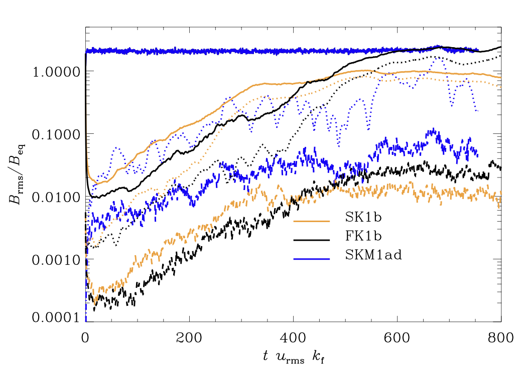
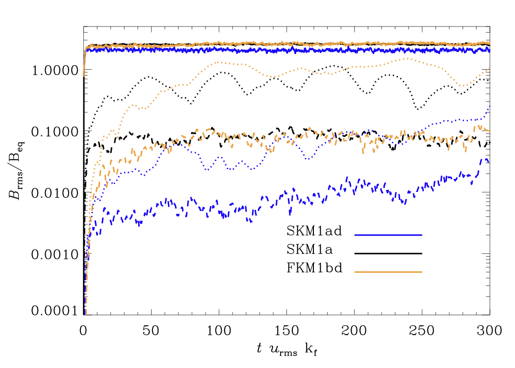
Figure 1: Time evolution of rms and mean magnetic field strengths from different runs. Top: comparison of a higher–$\mbox{\rm Re}_{\rm M}$ FK (black) and SK (orange) run, and a lower-$\mbox{\rm Re}_{\rm M}$ decimated SKM run (blue). Bottom: comparison of SKM runs with ${\cal A}=1$, with standard (black, Run SKM1a) and decimated (blue, Run SKM1ad) forcing. Solid – $B_{\rm rms}$, dotted – $\overline{B}_{y,{\rm rms}}$, dashed – $\overline{B}_{x,{\rm rms}}$.

Finally, we repeat the simulations, labeled “a” ($\mbox{\rm Pr}_{\rm M}=10/3$), with the same parameters, but using the magnetic forcing in addition to the kinetic one, so that the same rms velocity is obtained as in the kinetically forced cases. This set of parameters should very closely correspond to the case studied in Figure 9(d) of Squire & Bhattacharjee (2015b). As seen there, too, we observe a nearly immediate appearance (during the first five turnover times) of a strong $\overline{B}_{y}$ as is shown for Run SKM1a in Figure 1, lower panel. Although Squire & Bhattacharjee (2015b) did not show the evolution of $\overline{B}_{x}$, our results indicate that $\overline{B}_{y}$ arises due to the action of the strong shear on $\overline{B}_{x}$. After the initial rapid growth, we do not see any further increase of $\overline{B}_{x}$ while linear growth up to $tu_{\rm rms}k_{\rm f}\approx 170$ and quasi-regular oscillations occur in $\overline{B}_{y}$. Hence, we are not able to report a growth rate for Run SKM1a in Table LABEL:models, and also not for the larger-${\cal A}$ runs SKM4a, SKM8a and SKM16a for the same reason. We note that now the energy in the magnetic fluctuations is dominating over the energy in the mean field, with roughly 70% of the total contained in the former.

From Figure 2, middle panel, we see that, again, the $k_{z}/k_{1}=1$ vertical Fourier mode is the preferentially excited one, although the patterns seen in the $zt$ plots are much more short-lived and erratic in time than in the kinetically forced counterpart SK1a (same figure, top panel). Remarkably, there is no kinematic stage, but the large-scale pattern appears nearly instantly. (Note that the whole time range shown for Run SKM1a is roughly as long as the kinematic range exhibited by Run SK1b.) The appearance and evolution of $\overline{B}_{y}$ also disagree with the results of Squire & Bhattacharjee (2015b), who observed a much less erratic pattern to arise in a closely matching parameter regime — see their Figure 9(d).

The rapidly emerging mean fields in the magnetically and kinetically forced runs are related to the standard forcing scheme used in all the simulations presented so far. Even if this scenario could be regarded as a genuine dynamo instability, its investigation is out of the scope of our current numerical setup, because obviously much higher cadence in time should be used in an attempt to follow the possible kinematic stage. Also, the simulations should be started from a fully matured turbulent MHD background state, because currently the mean-field growth occurs during the initial transient state, where even turbulence itself is not yet saturated.

Hence, instead of fully dwelling on the cause of the rapid initial growth, we turn to using the decimated forcing with $k_{\min}/k_{1}=2$, and repeat Run SKM1a as a decimated version, now denoted SKM1ad and shown in the lower panel of Figure 1 (blue lines). We still see the rapid appearance of the mean fields, but their magnitudes are now much lower than in the case of our standard forcing, plotted with black lines in the same figure for comparison. After the rapid excitation phase, we observe a slow exponential growth of both $\overline{B}_{x}$ and $\overline{B}_{y}$, reminiscent of the dynamo instability seen in the FK and SK runs. The growth rate is now larger than in the kinetically forced counterparts FK1a and SK1a — see Table LABEL:models; when compared with the higher-$\mbox{\rm Re}_{\rm M}$ runs FK1b and SK1b, as can be seen from the upper panel of Figure 1, the growth rates are nearly equal. We also produced three more runs with varying aspect ratio ${\cal A}$ (SKM1ad, SKM8ad, and SKM16ad), and notice that the growth rate is increasing with ${\cal A}$ up to 8, but then decreases again. We further performed a magneto-kinetically forced FMHD run, where rapidly emergent mean fields are seen in spite of using the decimated forcing (see the bottom panel of Fig. 2, showing Run FKM1bd, with parameters corresponding roughly to Runs FK1b and SKM1ad). The emerging large-scale field structures are very similar to those in the magneto-kinetically forced SMHD cases, but less coherent than in the kinetically forced FMHD case. Similar to the SMHD cases with standard forcing, the growth rates are difficult to estimate, but we do note that the dynamo is now easier to excite than in the kinetically forced FMHD case, where the large-scale field emerged only at 600 turnover times instead of a few tens. Hence, we cannot confirm the finding of Squire & Bhattacharjee (2015b) that more coherent structures emerge when one goes from kinetic to magnetic forcing, as was the case in their incompressible study.

Based on these runs with different forcings, we propose that the slow dynamo instability could have been drowned by the stronger initial mean fields when forced with the standard forcing. Although the growth rate of the dynamo instability is similar to the kinetically forced cases, and the wavenumber of the dynamo instability are the same in both cases, the change of the growth rate as function of the aspect ratio of the box indicates that some key properties of the dynamo instability do change when magnetic forcing is used. In the next section we make an attempt to investigate what exactly has changed by measuring the turbulent transport coefficients in the systems with the relevant TFM variant.

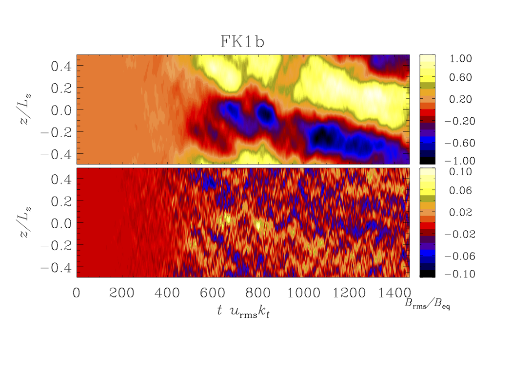
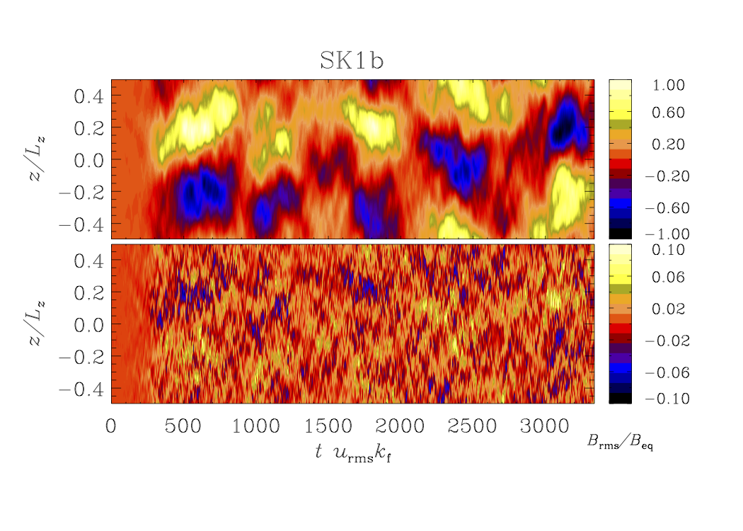
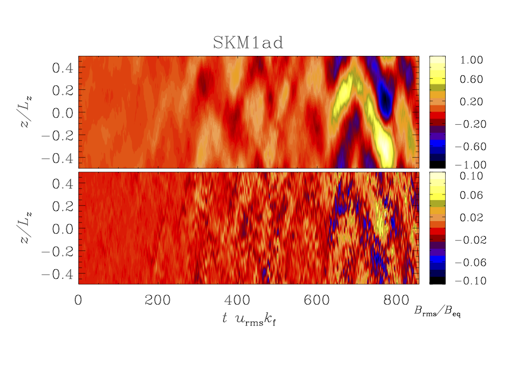
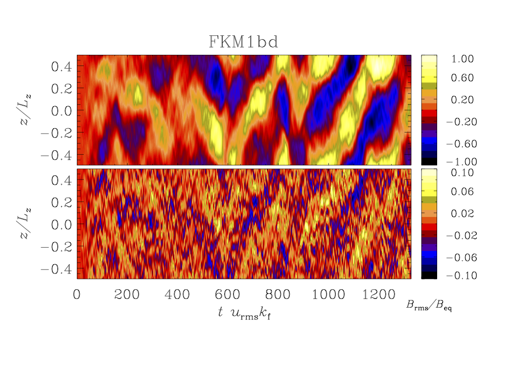
Figure 2: Butterfly ($zt$) diagrams of $\overline{B}_{y}$ (upper plot in each panel) and $\overline{B}_{x}$ (lower plot in each panel). Run FK1b is kinetically forced FMHD, Run SK1b is kinetically forced SMHD, SKM1a magneto-kinetically forced SMHD, SKM1ad its counterpart with decimated forcing, and FKM1bd is a magneto-kinetically forced run in FMHD, with parameters close to SKM1ad and FK1b and decimated forcing.

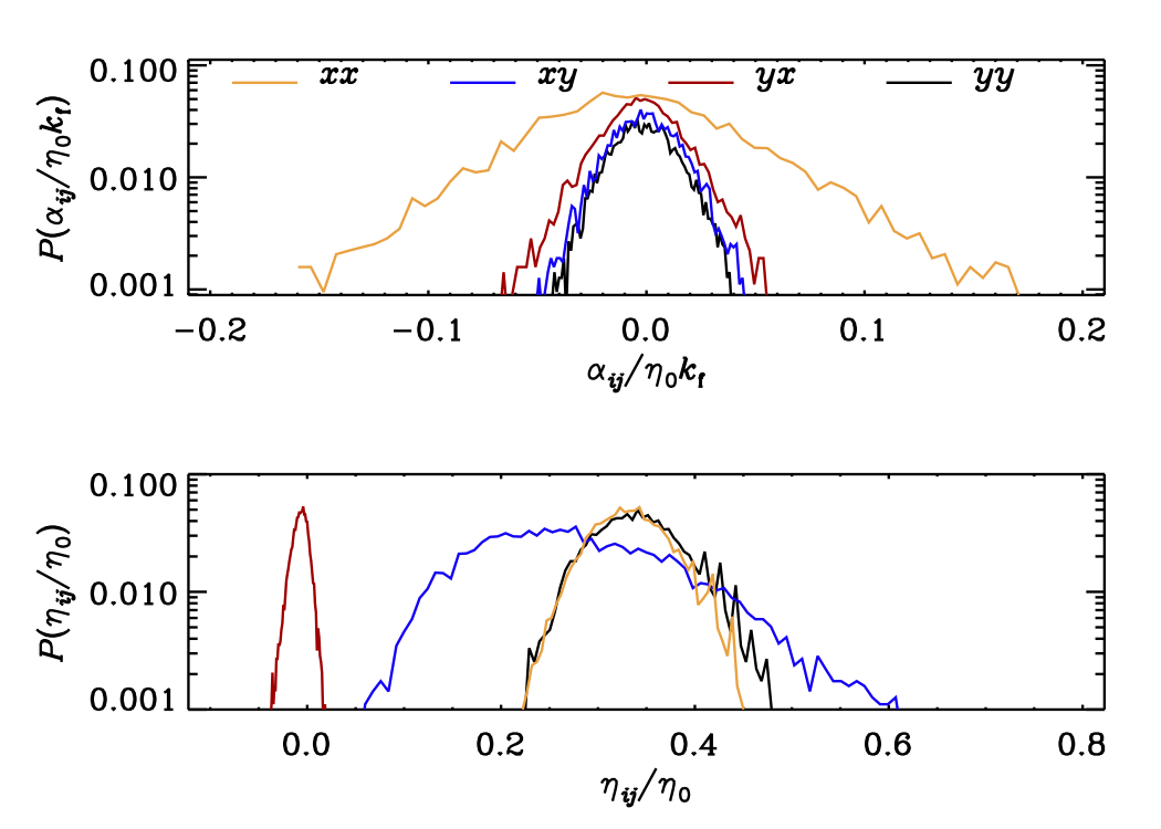
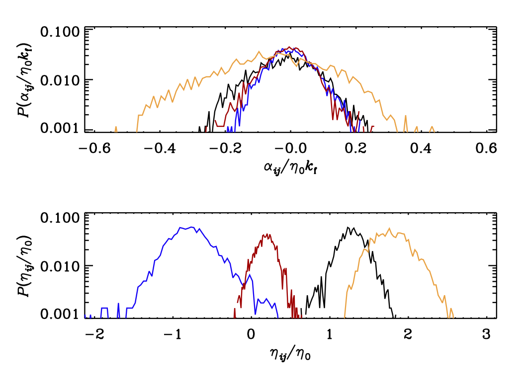
Figure 3: Probability density functions of all turbulent transport coefficients. Top: $\alpha_{ij}$, bottom: $\eta_{ij}$. Left: kinetically forced SMHD Run SK1b, right: magneto-kinetically forced SMHD Run SKM1a.

3.2 Turbulent transport coefficients

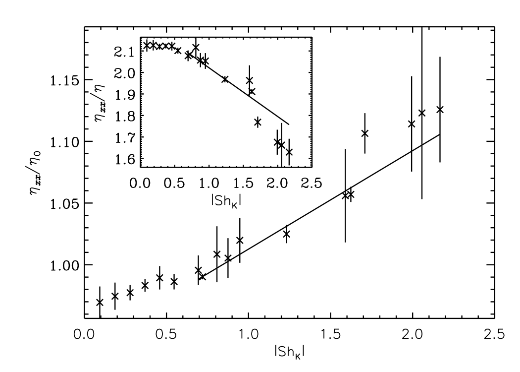
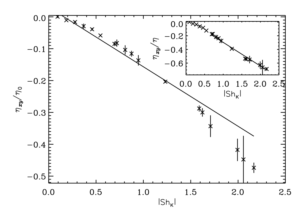
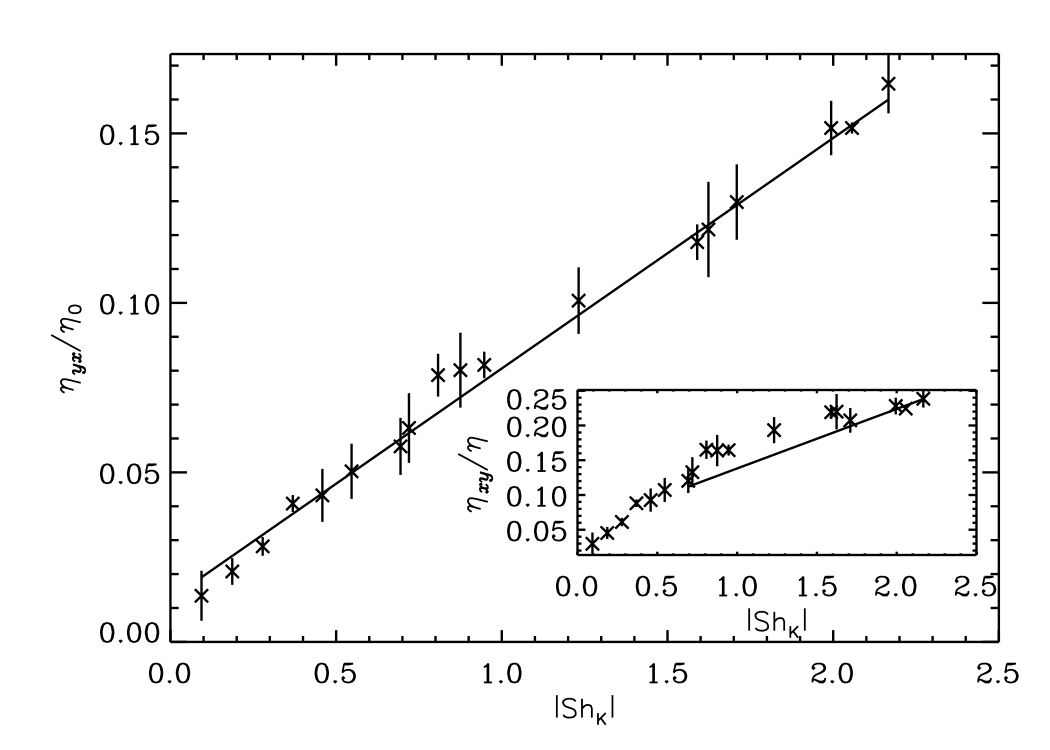
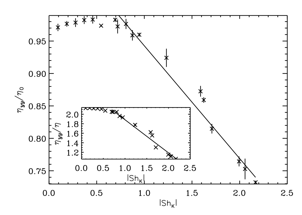
Figure 4: Dependence of the turbulent diffusivity tensor components, measured with NLTFM, on the shear number in the magneto-kinetically forced cases. In the big plots we normalize to the SOCA estimate $\eta_{0}$, while in the insets to the molecular diffusivity $\eta$.

Table 2: Summary of the runs with varying shear.

Run	$\mbox{\rm Sh}_{\rm K}$	$\eta_{xx}/\eta_{0}$	$\eta_{yy}/\eta_{0}$	$\eta_{yx}/\eta_{0}$	$\eta_{xy}/\eta_{0}$	$\alpha_{\rm rms}/(\eta_{0}k_{\rm f})$	$\eta_{\rm rms}/\eta_{0}$
SKM1a001	$-$0.094	2.125$\pm$0.028	2.129$\pm$0.012	0.030$\pm$0.016	$-$0.001$\pm$0.009	0.094$\pm$0.015	0.137$\pm$0.050
SKM1a002	$-$0.187	2.126$\pm$0.024	2.131$\pm$0.009	0.045$\pm$0.009	$-$0.023$\pm$0.003	0.101$\pm$0.029	0.142$\pm$0.066
SKM1a003	$-$0.278	2.120$\pm$0.023	2.123$\pm$0.015	0.061$\pm$0.006	$-$0.035$\pm$0.009	0.092$\pm$0.034	0.137$\pm$0.036
SKM1a004	$-$0.369	2.123$\pm$0.011	2.121$\pm$0.013	0.088$\pm$0.005	$-$0.063$\pm$0.017	0.096$\pm$0.014	0.153$\pm$0.043
SKM1a005	$-$0.458	2.122$\pm$0.020	2.109$\pm$0.013	0.093$\pm$0.017	$-$0.084$\pm$0.009	0.081$\pm$0.033	0.147$\pm$0.047
SKM1a006	$-$0.547	2.101$\pm$0.013	2.074$\pm$0.003	0.107$\pm$0.017	$-$0.125$\pm$0.005	0.088$\pm$0.032	0.164$\pm$0.071
SKM1a007	$-$0.649	2.077$\pm$0.025	2.051$\pm$0.007	0.120$\pm$0.018	$-$0.177$\pm$0.024	0.091$\pm$0.027	0.173$\pm$0.068
SKM1a008	$-$0.719	2.084$\pm$0.004	2.046$\pm$0.023	0.133$\pm$0.022	$-$0.173$\pm$0.014	0.084$\pm$0.019	0.173$\pm$0.081
SKM1a009	$-$0.808	2.116$\pm$0.048	2.049$\pm$0.016	0.165$\pm$0.013	$-$0.218$\pm$0.024	0.077$\pm$0.032	0.196$\pm$0.074
SKM1a01	$-$0.873	2.057$\pm$0.033	1.962$\pm$0.016	0.164$\pm$0.023	$-$0.237$\pm$0.031	0.081$\pm$0.034	0.196$\pm$0.083
SKM1a011	$-$0.947	2.053$\pm$0.037	1.932$\pm$0.006	0.165$\pm$0.008	$-$0.275$\pm$0.019	0.080$\pm$0.031	0.197$\pm$0.073
SKM1a015	$-$1.226	1.968$\pm$0.014	1.775$\pm$0.027	0.193$\pm$0.019	$-$0.391$\pm$0.033	0.074$\pm$0.027	0.219$\pm$0.094
SKM1a02	$-$1.582	1.963$\pm$0.070	1.622$\pm$0.015	0.219$\pm$0.010	$-$0.535$\pm$0.007	0.067$\pm$0.018	0.233$\pm$0.068
SKM1a021	$-$1.623	1.911$\pm$0.011	1.553$\pm$0.008	0.220$\pm$0.025	$-$0.542$\pm$0.018	0.064$\pm$0.030	0.238$\pm$0.103
SKM1a025	$-$1.709	1.769$\pm$0.026	1.303$\pm$0.012	0.207$\pm$0.018	$-$0.549$\pm$0.055	0.058$\pm$0.030	0.223$\pm$0.083
SKM1a031	$-$1.985	1.676$\pm$0.058	1.150$\pm$0.011	0.228$\pm$0.012	$-$0.628$\pm$0.053	0.056$\pm$0.024	0.238$\pm$0.069
SKM1a0325	$-$2.057	1.662$\pm$0.103	1.114$\pm$0.024	0.224$\pm$0.002	$-$0.663$\pm$0.110	0.050$\pm$0.014	0.236$\pm$0.035
SKM1a035	$-$2.156	1.630$\pm$0.062	1.060$\pm$0.004	0.238$\pm$0.013	$-$0.686$\pm$0.023	0.052$\pm$0.012	0.248$\pm$0.083

Note: Forcing wavenumber $k_{\rm f}/k_{1}=5$. The magnetic Reynolds number, $\mbox{\rm Re}_{\rm M}$, varies from 1.4 (for weak shear) to 2.1 (for strong shear), and the Lundquist number, Lu, from 4.2 (for weak shear) to 4.8 (for strong shear). ${\cal A}=1$ in all the runs.

3.2.1 Cases of strong shear

In this subsection we compare cases of strong shear in kinetically forced FMHD and SMHD, and magneto-kinetically forced SMHD, measured with the appropriate variant of the TFM. We choose $S=-25/T_{\nu}$, which, with the selected amplitude of the forcing, results in the shear number $\mbox{\rm Sh}_{\rm K}\approx-1.6$, indicating a strong influence of shear on the system. This setup closely matches the cases investigated by Squire & Bhattacharjee (2015b).

First we use the QKTFM to measure the turbulent transport coefficients in the kinetically forced FMHD cases, the results being presented in Table LABEL:models. We measure zero mean in all $\alpha$ components, hence we tabulate only the rms values of the $\alpha$ fluctuations: $\alpha_{\rm rms}=\langle\alpha_{ij}^{2}\rangle_{t}^{1/2}$. The same applies to all other runs studied here. In the low-$\mbox{\rm Re}_{\rm M}$ cases (FK1a, FK8a) we measure relatively isotropic diagonal components of the $\eta$ tensor, positive and somewhat smaller values of $\eta_{xy}$ and much smaller positive values of $\eta_{yx}$. In these cases, no indication of LSD instability is seen.

In the high $\mbox{\rm Re}_{\rm M}$ cases (FK1b and FK8b), the diagonal components of $\bm{\eta}$ have, as expected, higher magnitudes, showing only mild anisotropy, as in the low-$\mbox{\rm Re}_{\rm M}$ cases, such that $\eta_{xx}$ somewhat exceeds $\eta_{yy}$. $\eta_{xy}$ is increased with respect to the diagonal components, reaching roughly 75% of their magnitudes. $\eta_{yx}$ is still positive, and decreases in magnitude. In these cases we see LSD action, but with $\eta_{yx}$ being positive it seems unlikely that the dynamo is of SC-effect origin, in agreement with previous numerical studies (Brandenburg et al., 2008; Yousef et al., 2008b; Singh & Jingade, 2015). They did not consider as large values of the shear parameter as here, so we can now extend this conclusion to the strong-shear regime. This is consistent with a series of earlier analytical works that treated shear non-perturbatively and found no evidence of SC-assisted LSD (Sridhar & Subramanian, 2009a, b; Sridhar & Singh, 2010; Singh & Sridhar, 2011). We analyze the possible dynamo driving mechanism in more detail in Sect. 3.3.

Next we turn to the kinetically forced SMHD cases, analyzed with both the QKTFM and NLTFM, yielding consistent results, as discussed in Appendix B.2. The biggest difference from FMHD is that all $\bm{\eta}$ components are systematically smaller in SMHD, and moreover, $\eta_{yx}$ has changed sign to negative values, being statistically significant within errors; see Table LABEL:models. Also, the rms $\alpha$ values are similar or a bit larger. In the face of the turbulent transport coefficients, it seems understandable that for the low-$\mbox{\rm Re}_{\rm M}$ cases the LSD is excited in SMHD but not in FMHD, because the diffusive coefficients are lower, while the inductive ones are larger. Also, the sign of $\eta_{yx}$ would now be favorable to enable the SC effect to support an LSD. Further, it is noteworthy that the diagonal components of $\bm{\eta}$ become more notably anisotropic, but now $\eta_{yy}$ mostly exceeds $\eta_{xx}$. In Figure 3, we show for Run SK1b the probability density distributions of all tensor components. The diagonal $\bm{\alpha}$ components exhibit larger values than the off-diagonal ones, $\alpha_{xx}$ being especially strong. The off-diagonal components are very similar to each other. The diagonal $\eta$ components are close to being isotropic. $\eta_{yx}$ is fluctuating tightly around zero, and exhibits a very small negative mean. The distribution of $\eta_{xy}$ is broad, but always in the positive.

Lastly, we turn to the magneto-kinetically forced SMHD cases, analyzed with the NLTFM. In the low-$\mbox{\rm Re}_{\rm M}$ runs, all components of $\bm{\eta}$ show larger magnitudes than in the kinetically forced cases. Its diagonal components now show very strong anisotropy, with $\eta_{xx}$ being again dominant over $\eta_{yy}$ as in the FMHD cases. $\eta_{xy}$ has changed sign to negative values, while $\eta_{yx}$ is again positive. The rms values of $\alpha$ and $\eta$ are (mostly) increased, in particular those of the latter. The probability density functions of the transport coefficients, shown in the right column of Figure 3, clearly demonstrate the anisotropy of the diagonal components of $\bm{\eta}$ and the sign change of $\eta_{xy}$ to large negative values, with $\eta_{yx}$ now exhibiting a clearly positive mean with some negative values as well. The $\alpha$ components are very similar to the kinetically forced SMHD case, with $\alpha_{xx}$ attaining much larger values than $\alpha_{yy}$ and the off-diagonal components. The positive sign of $\eta_{yx}$ rules out the existence of an SC-effect dynamo in these cases. As will be discussed in detail in Sect. 3.3, the $\alpha$ and $\eta$ fluctuations then remain as possible candidates to provide the necessary ingredients for an LSD.

3.2.2 Dependence on the shear parameter

In this section we report on the dependence of the turbulent transport coefficients on the shear number $\mbox{\rm Sh}_{\rm K}$ in runs with magneto-kinetical forcing. We list our runs, their basic diagnostics, and the turbulent transport coefficients measured with the NLTFM in Table LABEL:Shmodels. As the standard forcing was used here, we did not see any exponential growth in the evolution of the mean fields; see Sect. 3.1 for a reasoning. Hence, no growth rates are reported, and we note that all the transport coefficients are measured from a stage where the mean magnetic fields are dynamically significant. As can be seen from the listed Lu, these runs are all strongly magnetically dominated, likely because the small-scale magnetic fields are primarily generated by the magnetic forcing. Our purpose is to scan a wider range of shear strengths for possible occurrences of a negative $\eta_{yx}$ as a function of $\mbox{\rm Sh}_{\rm K}$, which could enable an SC-driven LSD. The results are depicted in Figure 4, where we present the $\bm{\eta}$ components in two different normalizations. As can be seen, with weak shear ($|\mbox{\rm Sh}_{\rm K}|<0.5$), the diagonal components of $\bm{\eta}$ are isotropic, while with stronger shear, anisotropy develops such that in the SOCA normalization, $\eta_{xx}$ increases linearly while $\eta_{yy}$ decreases linearly. Normalizing to molecular diffusivity, both components are decreasing linearly, $\eta_{xx}$ less steeply than $\eta_{yy}$. For weak shear, $\eta_{yx}$ adopts small positive values, which keep increasing linearly with shear in the SOCA normalization. The linear trend is less clear in the molecular diffusivity normalization. Furthermore, $\eta_{xy}$ attains weakly negative values for weak shear, and increasingly negative ones for strong shear. The trend is very close to linear when molecular diffusivity is used for normalization. Hence, we find no possibility for an MSC-effect-driven dynamo at any shear number investigated.

The dependences of $\eta_{ij}$ on shear, as obtained here, are in broad agreement with the results of Singh & Sridhar (2011) based on an analytical study in which arbitrarily large values of the shear parameter $S$ could be explored; see references therein for more discussion. The two off-diagonal components $\eta_{xy}$ and $\eta_{yx}$ were found to start from zero at zero shear and, while the more relevant $\eta_{yx}$ increases with $|S|$ to remain positive, $\eta_{xy}$ behaves in a more complicated manner than found here, exhibiting both signs depending on the value of $S$: It decreases with increasing $|S|$ to become negative up to a certain value of shear, as in the present work; we refer the reader to Singh & Sridhar (2011) for more detail on its behavior at larger $\left|S\right|$.

3.2.3 Dependence on the aspect ratio

We have studied the dependence of the turbulent transport coefficients on the aspect ratio ${\cal A}$ of the domain in the three different cases (FMHD, SMHD with kinetic or magneto-kinetic forcing) with fixed shear parameter $S=-25/T_{\nu}$. The measured growth rate of the rms magnetic field, which coincides with those of of $\overline{B}_{x}$ and $\overline{B}_{y}$ except for standard magnetic forcing, and the measured turbulent transport coefficients are listed in Table LABEL:models; see runs with labels 4, 8, and 16, indicating ${\cal A}$.

In the kinetically forced FMHD and SMHD cases, the growth rate of the magnetic field is largely independent of the aspect ratio of the box, indicating that always one and the same dynamo mode is growing. We also measure the vertical wavenumber $k_{z}$ of the fastest growing dynamo mode in the kinematic stage (see Table LABEL:dynamonumbers), which supports this conclusion, as we see the $k_{z}/k_{1z}$ increasing proportional to ${\cal A}$. The turbulent transport coefficients do not show a marked dependence on ${\cal A}$ either.

In SMHD with standard magneto-kinetic forcing, the situation is somewhat different. As we cannot draw conclusions on the growth rate of the magnetic field in these cases, we use the corresponding cases with decimated forcing as a guideline. The latter (see Table LABEL:models, runs with label ending in “d”) show that the growth rate is increasing with ${\cal A}$ up to 8 and then decreases again in the tallest box. In Figure 5 we show $\eta_{yx}$ as a function of ${\cal A}$. It can be seen that the magnitudes of the turbulent transport coefficients change somewhat as a function of the aspect ratio, although the magnitudes seem to saturate for the tallest box. The diagonal components grow in magnitude, $\eta_{xx}$ somewhat more than $\eta_{yy}$ making the anisotropy in the turbulent diffusivity even larger. The negative values measured for $\eta_{xy}$ tend to get weaker in taller boxes. The positive values of $\eta_{yx}$ increase with ${\cal A}$, hence we see no tendency for larger boxes to be more favorable for the SC dynamo. The fluctuating $\alpha$ and $\eta$ behave similarly, with their magnitudes first increasing, but then decreasing for the tallest box. The decimated forcing cases show a similar trend for ${\cal A}=4,8,$ and $16$ (SKM4ad, SKM8ad, and SKM16ad) while the case ${\cal A}=1$ (SKM1ad) shows higher values of the transport coefficients not agreeing with this trend.

As the number of grid points is proportional to ${\cal A}$ at fixed resolution, resource limitations dictated to integrate the large-${\cal A}$ runs only over significantly shorter time spans. However, as we have discussed above, the mean fields grow initially very rapidly in all runs with standard forcing, irrespective of the aspect ratio. Hence, an effect of the different integration times on the values of transport coefficients can be ruled out.

One could also speculate that some spatio-temporal nonlocality (see, e.g., Rheinhardt & Brandenburg, 2012) might come into play with magnetic forcing, but when choosing our forcing wavenumbers, we have taken care of $k_{\rm f}$ being scaled with respect to the vertical extent of the computation domain such that the forcing wavenumber remained constant. Our procedure, however, does not take into account non-local effects in any way.

The dependence of the growth rate on the aspect ratio could also be due to different dynamo modes being excited in boxes of different size. This was found by Shi et al. (2016) in a similar context, but including rotation, in which case the turbulence was self-sustained (i.e., not driven as in our study) by the magnetorotational instability (MRI). They found the dynamo to be more efficient in taller boxes, and interpreted this by having “cut out” some modes in the smaller boxes. However, determining the vertical wavenumber of the fastest growing mode in the kinematic stage for the decimated forcing runs, we find no evidence for this. As the turbulence in the cases with standard and decimated forcing is different though, we cannot regard this as completely conclusive evidence that rules out this scenario.

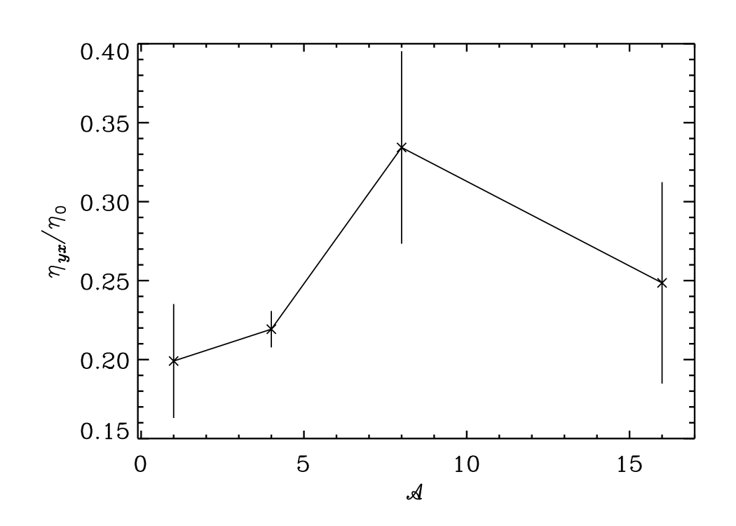
Figure 5: Dependence of $\eta_{yx}$ on the aspect ratio ${\cal A}$ for SMHD cases with standard magneto-kinetic forcing.

3.3 Interpretation of the dynamo instability

For SC-effect-driven dynamos, the dispersion relation from linear stability analysis for solutions, exponential in time, reads (see, e.g., Brandenburg et al., 2008)

$$\frac{\lambda_{\pm}}{\eta_{\rm T}k_{z}^{2}}=-1\pm\frac{1}{\eta_{\rm T}}\sqrt{\left(\frac{S}{k_{z}^{2}}+\eta_{xy}\right)\eta_{yx}+\epsilon^{2}},$$ (23)

with $\eta_{\rm T}=\eta+\eta_{\rm t}$, $\eta_{\rm t}=\left(\eta_{xx}+\eta_{yy}\right)\!/2$, $\epsilon=\left(\eta_{xx}-\eta_{yy}\right)\!/2$. A necessary and sufficient condition for growing solutions is that the radicand is positive, and larger than $\eta_{\rm T}^{2}$. In other words (for $\epsilon\approx 0$)

$$D_{\eta S}\equiv\left(\frac{S}{k_{z}^{2}}+\eta_{xy}\right)\frac{\eta_{yx}}{\eta_{\rm T}^{2}}>1,$$ (24)

which is often further simplified by ignoring the contribution from $\eta_{xy}$, because it is considered negligible in comparison to $S/k_{z}^{2}$. This also holds for the systems studied here, but we note that in all our cases, $\eta_{xy}$ is much larger than $\eta_{yx}$ and in the kinetically forced cases it is even comparable to the diagonal components. Hence, setting it to zero, as has been done in some fitting experiments to determine the turbulent transport coefficients (see, e.g., Shi et al., 2016), is not justified. Especially in the magneto-kinetically forced cases with strong shear, the assumption $\epsilon\approx 0$, made in those fitting experiments, breaks down, too.

Table 3: Dynamo numbers for the runs in Table LABEL:models.

Run $\!\!\!\!\!\!\!\!{k_{z}/k_{1z}}$ $D_{\eta S}$ $D_{\eta_{\rm rms}S}\!\!\!\!$ $D_{\alpha S}$ FK1a 1* $-1.4$ 1.6 2.8 FK1b 1 $-3.9$ 5.3 19.2 FK8a 9* $-1.0$ 1.1 0.7 FK8b 9 $-2.8$ 3.2 4.7 SK1a 1 0.1 0.3 2.9 SK1b 1 2.7 4.2 25.5 SK4a 4 0.1 0.2 1.5 SK4b 4 1.3 2.6 14.6 SK8a 4 0.5 0.7 8.2 SK8b 9 2.1 2.4 3.6 SKM1a 1* $-2.7$ 3.3 6.8 SKM4a 4* $-2.9$ 3.0 3.0 SKM8a 4* $-12.2$ 12.7 13.1 SKM16a 9* $-9.4$ 9.9 7.5 SKM1ad 1 $-4.0$ 7.2 19.6 SKM4ad 4 $-3.4$ 4.1 9.8 SKM8ad 8 $-5.7$ 6.1 6.8 SKM16ad 15 $-4.7$ 4.9 5.1

Note. Runs marked with * are not dynamo active, hence the wavenumber of the growing dynamo mode is extracted from other runs of similar aspect ratio.

For incoherent $\alpha$-shear-driven dynamos, the relevant dynamo number reads (see, e.g., Brandenburg et al., 2008)

$$D_{\alpha S}=\frac{\alpha_{\rm rms}\left|S\right|}{\eta_{\rm T}^{2}k_{z}^{3}},$$ (25)

where usually only the fluctuations of $\alpha_{yy}$ are considered for $\alpha_{\rm rms}$. They determined the critical $D_{\alpha S}$ to be $\approx 2.3$ for white-noise $\alpha$ fluctuations. Brandenburg et al. (2008) also reported that the diagonal and off-diagonal components of the $\alpha$ tensor were nearly equal. In the SMHD cases studied here, this is no longer the case, as is shown in Figure 3, where $\alpha_{xx}$ dominates.

Brandenburg et al. (2008) also discussed the possibility of a contribution from an incoherent SC effect by fluctuations of $\eta_{yx}$ with vanishing mean. They studied a model where both incoherent effects were acting together, the incoherent $\alpha$ effect mainly through $\alpha_{yy}$ while the incoherent SC effect through $\eta_{yx}$ is described by the dynamo number

$$D_{\eta_{\rm rms}S}=\frac{\eta_{yx,\rm rms}\left|S\right|}{\eta_{\rm T}^{2}k_{z}^{2}}.$$ (26)

They found that for small $D_{\eta_{\rm rms}S}$ the critical dynamo number, detected for the incoherent $\alpha$ effect alone, was not much altered, while for higher values that critical number could be clearly reduced. Hence, to decide which dynamo effect is at play in systems with large fluctuations, one should always consider the dynamo numbers for both incoherent effects simultaneously.

Moreover, the presence of an additional coherent SC effect can alter the dynamo excitation condition, which we now account for by adding a term from a coherent $\eta_{yx}$ to the simplified zero-dimensional (0D) dynamo model of Brandenburg et al. (2008); see their Appendix C. The equation solved is the linear mean-field induction equation

$$\partial_{t}\overline{\bm{A}}=-S\overline{A}_{y}\hat{{\bm{x}}}+\overline{\mbox{\boldmath${\cal E}$}}{}-\eta{\overline{\bm{J}}},$$ (27)

where the mean EMF now reads

$$\overline{\cal E}{}_{i}=\alpha_{ij,\rm inc}(t)\overline{B}_{j}-\left(\eta_{yx,\rm inc}(t)+\eta_{yx}\right)\delta_{i2}\overline{J}_{x}.$$ (28)

The incoherent effects are modeled with $\delta$-correlated noise in time having zero means and standard deviations equal to the respective rms values, while the coherent contribution from $\eta_{yx}$ is constant. By the ansatz ${\overline{\bm{A}}}\sim\exp({\rm i}k_{z}z)$, Eq. (27) turns into the 0D model, with governing parameters $D_{\alpha S}$, $D_{\eta S}$, and $D_{\eta_{\rm rms}S}$, defined above.

We have verified that dynamo action in this model without any incoherent effects takes place when $D_{\eta S}$ is exceeding unity, as expected from the stability criterion (24). We compute new stability maps in the $D_{\eta_{\rm rms}S}\,$–$\,D_{\alpha S}$ plane for a series of dynamo numbers $D_{\eta S}$, in the range $[-1.5,2]$. These values are similar in magnitude as those realized in our simulations, although not covering the extremal values obtained in the magneto-kinetic forcing cases. These are shown in Figure 6, where panels (d) and (e) closely match the stability map of the incoherent effects alone (compare with Figure 12 of Brandenburg et al., 2008). As expected, adding a coherent SC effect with a positive $D_{\eta S}$ enhances the dynamo instability, especially by lowering the critical dynamo number for the incoherent $\alpha$-shear dynamo. This is seen through the shift of the stability line (white contours in Figure 6) to the left (toward smaller values of $D_{\alpha S}$) from (f) to (i). The incoherent SC dynamo threshold is also lowered, but the effect is more subtle, as seen through the much less dramatic shift of the stability boundary downward (toward smaller values of $D_{\eta_{\rm rms}S}$) in Figure 6, panels (f)–(i). For $D_{\eta S}>1$, the coherent SC effect alone would result in the excitation of a dynamo, but the presence of the incoherent effects causes small islands in which dynamo action is suppressed; see the dark red areas surrounded by the white contour in Figure 6, panels (g) and (h).

In the dynamo numbers (24)–(26) we also need the vertical wavenumber $k_{z}$ of the dynamo mode, which we determined from Fourier analysis of the mean fields during the kinematic phase of the dynamo. For those runs that are not dynamo-active, we used $k_{z}$ from a corresponding dynamo-active run with higher $\mbox{\rm Re}_{\rm M}$ (for kinetically forced runs) or a different forcing function (for magneto-kinetically forced runs), but the same aspect ratio (see Table LABEL:models), and we denote those runs for which we obtained $k_{z}$ from elsewhere with an asterisk in Table LABEL:dynamonumbers. We also note that, if the dynamo enters saturation, the kinematically preferred mode is not necessarily any longer present. Independent of the aspect ratio of the box, all the saturated models exhibit a magnetic field at the scale of the box or, in other words, at the smallest permissible wavenumber.

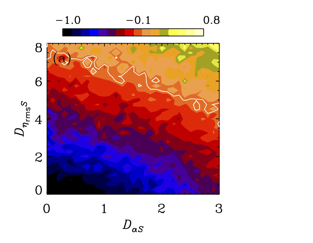
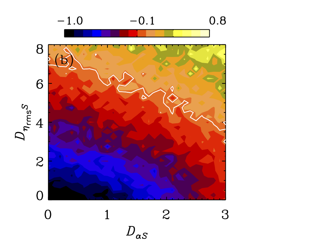
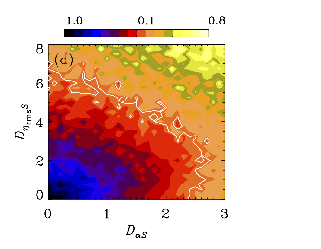
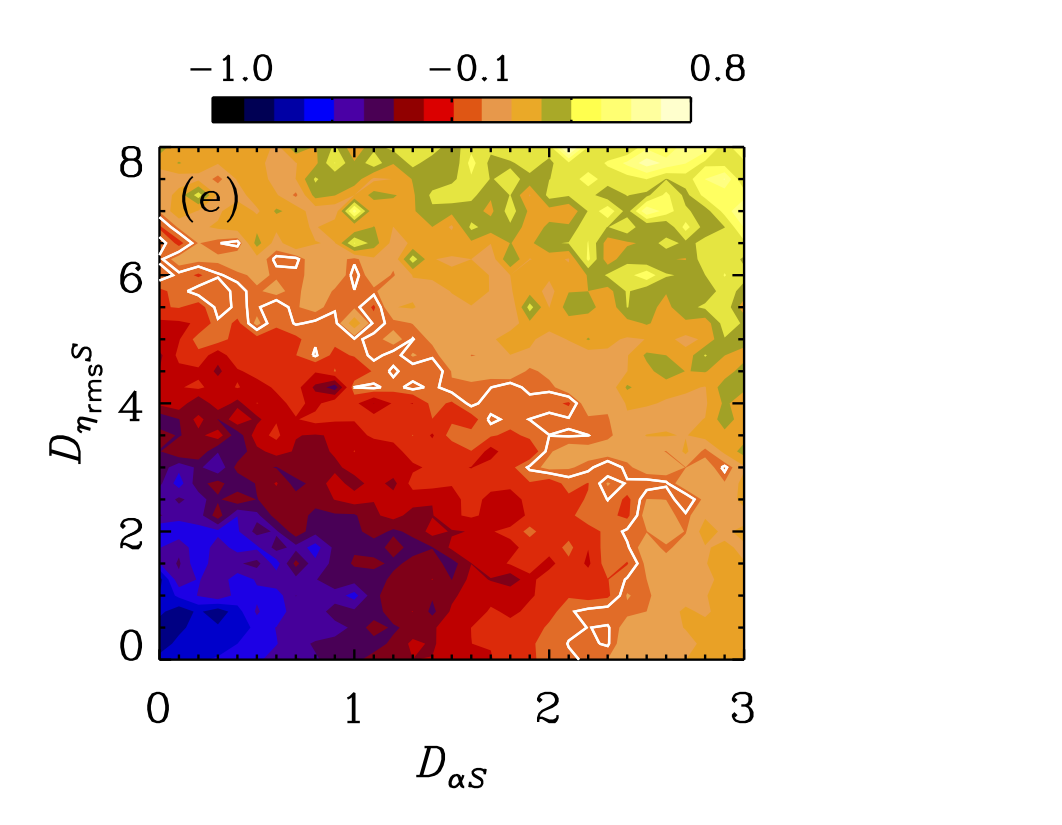
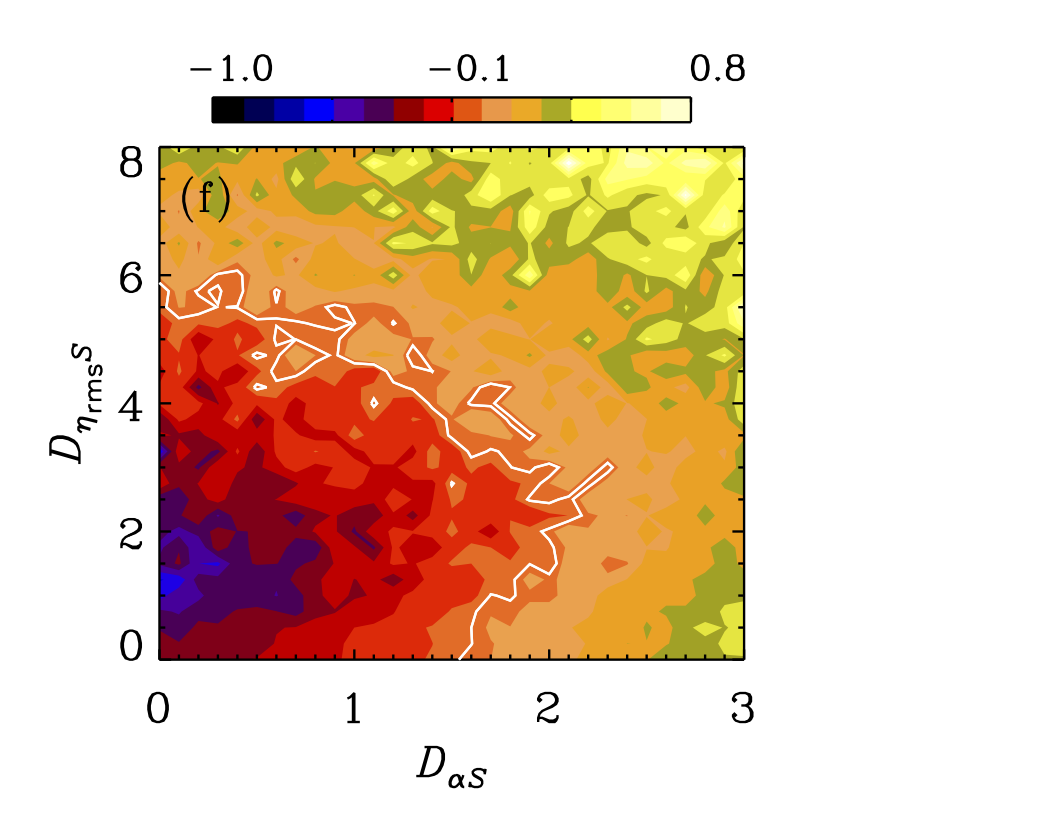
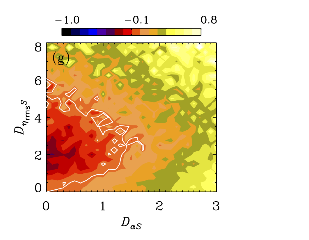
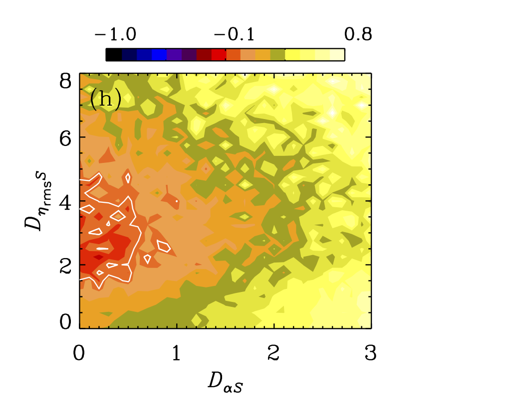
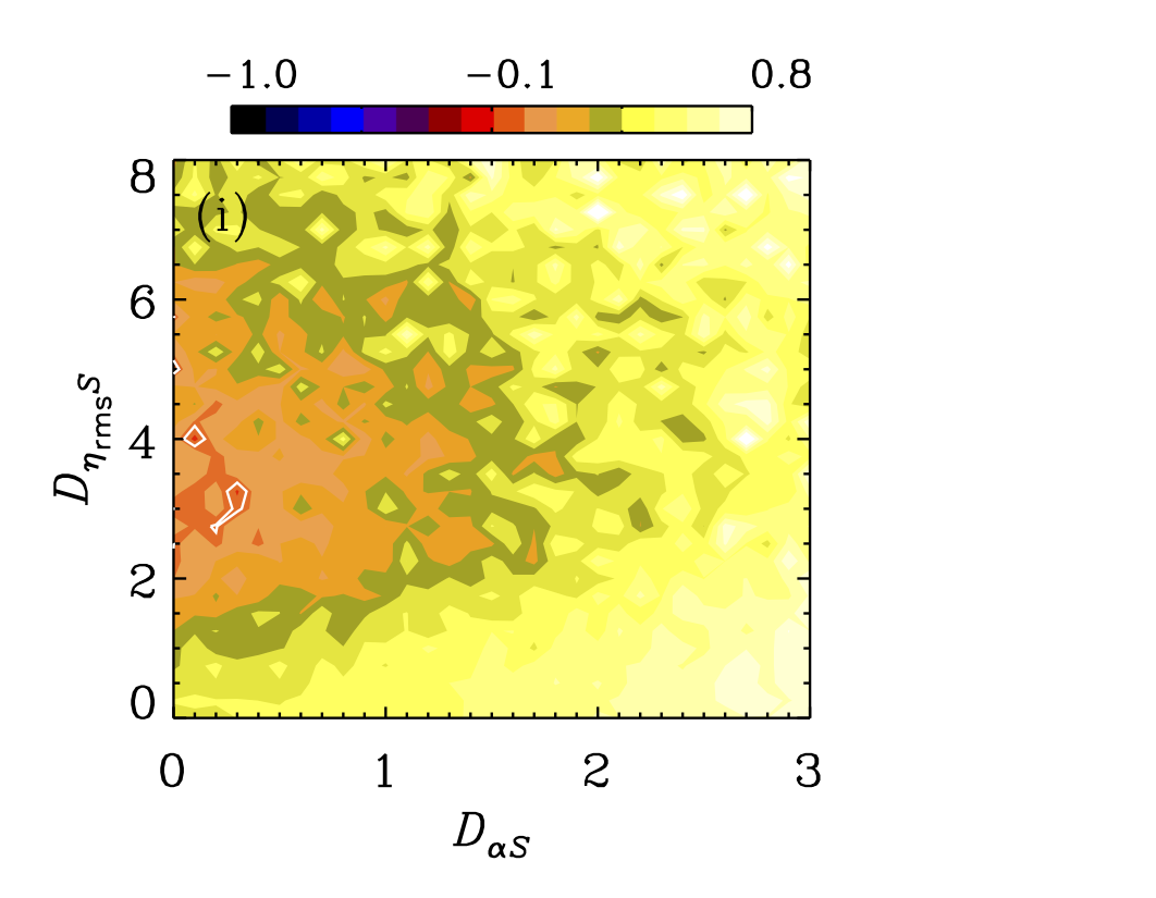
Figure 6: Stability diagrams for different values of $D_{\eta S}$: from top left to bottom right, -1.5,-1.0,-0.5,-0.1,0.1,0.5,1.0,1.5, and 2.0.
White: zero-growth-rate contour. Color scales: $\lambda/\eta_{\rm T}k_{z}^{2}$.

In the FMHD cases, we obtain negative $D_{\eta S}$ and incoherent SC dynamo numbers of similar magnitude, with $D_{\alpha S}$ tending to be larger than $D_{\eta_{\rm rms}S}$, especially in Run FK1b. In the case of Run FK8a, no dynamo action is seen, and none of the dynamo numbers predicts a dynamo either. In the other case without dynamo, Run FK1a, the $\eta$-related dynamo numbers predict no dynamo action, while $D_{\alpha S}$ alone would do so ($D_{\alpha S}=2.8>D_{\alpha S,\rm crit}=2.3$). Its critical value, however, can be increased in this case, mainly by the presence of the rather strong coherent SC effect with a negative dynamo number. The two dynamo-active cases have $D_{\alpha S}$ clearly above the critical value. Hence, the presence of moderate suppressing factors cannot prevent the dynamo instability. It clearly seems to be the incoherent $\alpha$-shear one in the FMHD cases, because $D_{\eta_{\rm rms}S}$ is far too small in this case.

In the kinetically forced SMHD cases, however, $\eta_{yx}$ is negative, allowing for the possibility of a coherent SC-effect dynamo. All our runs of this type are dynamo-active, but only the high-$\mbox{\rm Re}_{\rm M}$ cases exhibit supercritical $D_{\eta S}$ ($>1$). Except for the case of Run SK4a, the $D_{\alpha S}$ and $D_{\eta_{\rm rms}S}$ values indicate supercriticality for the incoherent dynamo instabilities, explaining again most of our findings. Run SK4a has a low positive $D_{\eta S}$, but also the incoherent effects are well below their critical dynamo numbers. The coherent SC effect could therefore assist the dynamo, but this effect should be negligible according to the 0D model. Hence, this dynamo remains unexplained with any dynamo scenario. Dynamo excitation is easier In the SMHD models than in the FMHD ones, which might indicate that the coherent SC effect assists dynamo action, but the SMHD simplifications could also be the cause.

In the magneto-kinetically forced SMHD cases, the dynamo numbers indicate stability against the MSC effect, but are all, according to individual 0D model runs (not presented here), supercritical for the incoherent dynamo effects, the incoherent SC effect being even more pronounced now than in the kinetically forced cases. Although the cases with standard forcing do not show exponential growth, their decimated forcing counterparts do so. Hence our interpretation here is that a dynamo is present in all the cases with magneto-kinetic forcing. Even though the coherent SC effect now exhibits larger negative dynamo numbers we find, by running individual 0-D models, that in all cases it should not be able to damp down the dynamo instability. Hence, again, the most likely mechanism for exciting the dynamo is the incoherent $\alpha$-shear effect, with supercritical $D_{\alpha S}$ in all cases. However, we cannot rule out the coexistence of an incoherent SC effect, as some runs also indicate supercriticality against it.

4 Conclusions

We have studied different types of sheared MHD systems with the quasi-kinematic (QKTFM) and nonlinear (NLTFM) test-field methods. In those cases studied with the NLTFM, we simplified the MHD equations neglecting the pressure gradient in the momentum equation, which allows us to ignore the equation for the fluctuating density in the test-field formulation, simplifying it somewhat. In the case of the full MHD equations studied with the QKTFM, we extend the previous results to even stronger shear, but still find no evidence for negative values of the $\eta_{yx}$ component that could lead to LSD action through the SC effect.

In kinetically forced magnetized burgulence (SMHD), we measure negative values of $\eta_{yx}$. Indeed, dynamo action with both radial and azimuthal magnetic field components growing exponentially at the same rate is found. The dynamo numbers for the coherent and the incoherent effects, based on the measured turbulent transport coefficients, however, when employed in a simplified 0D dynamo model, indicate that even in this case the dynamo is mainly driven by the incoherent $\alpha$ effect and shear, possibly assisted by the coherent SC effect.

In the case of systems with standard magneto-kinetic forcing, we do not find exponential growth of the mean magnetic field. When we repeat this experiment with a decimated forcing function, removing the smallest wavenumber components, exponential growth is recovered. Hence, in our interpretation, there is still a dynamo instability in the magneto-kinetically forced cases, but it becomes engulfed by the rapid growth of the mean field due the presence of these low wavenumbers in the forcing, preventing us from seeing the exponential growth of the mean field. The measured $\eta_{yx}$ are again positive and increasing as a function of the magnitude of shear and the aspect ratio of the box, and are therefore incapable of driving a dynamo through the MSC effect. This finding is compatible with our analytical derivation predicting a positive contribution to $\eta_{yx}$ in the case when the pressure term is neglected, albeit restricted to ideal MHD; see Appendix C. The computed dynamo numbers, compared against the 0D model, again indicate the most likely driver of the dynamo to be the incoherent $\alpha$ effect with shear.

We note that we have not investigated the magnetic Prandtl number ($\mbox{\rm Pr}_{\rm M}$) dependence of the magneto-kinetically forced cases although, according to the study of Squire & Bhattacharjee (2015a), $\mbox{\rm Pr}_{\rm M}$ has an influence on the magnitude of $\eta_{yx}$ (in their case always negative) such that its modulus decreases when $\mbox{\rm Pr}_{\rm M}$ is increasing. Their model includes both rotation and shear, and in addition they do not specify how $\mbox{\rm Re}_{\rm M}$ and Re changed when $\mbox{\rm Pr}_{\rm M}$ was changed. Hence, the applicability of these results to our case is uncertain, but studying the $\mbox{\rm Pr}_{\rm M}$ dependence is an important future direction. We also acknowledge that the simplified MHD equations used here prevent our conclusions from being generally applicable. Hence we cannot fully reject the postulated possibility of a dynamo driven by the MSC effect. The measurements should be repeated with the full MHD equations, analyzed with a fully compressible TFM, also solving for the density fluctuations.

Appendix A Comparison of standard and decimated forcing

To investigate the possible anisotropy due to the removal of all $|k_{x,y,z}|/k_{1}\leq k_{\rm min}/k_{1}$ from the forcing (decimation), we perform two hydrodynamic simulations without shear. Both runs were performed with $64^{3}$ grid points and $k_{\rm f}/k_{1}=5$, one without decimation and one with, using $k_{\rm min}/k_{1}=2$. All other parameters were the same and $u_{\rm rms}$ was similar in the two cases, with Mach number $\mbox{\rm Ma}=u_{\rm rms}/c_{\rm s}=0.002$ and $\mbox{\rm Re}=0.04$. In Figure 7 we show probability density functions (PDFs) of the three components of $\bm{u}$ from a snapshot of each run. These PDFs are normalized such that $\int P(u_{i})\,du_{i}=1$. We find that the PDFs of $u_{x}$, $u_{y}$, and $u_{z}$ are in both cases on top of each other, suggesting that the stochastic flows are nearly isotropic, at least in a statistical sense. Let us define the kurtosis, $\mbox{kurt}\,x$, of the distribution $P(x)$ as

$$\mbox{kurt}\,x=\frac{1}{\sigma^{4}}\int_{-\infty}^{\infty}(x-\overline{x})^{4}P(x)dx-3,$$ (A1)

where $\overline{x}$ and $\sigma$ are its mean and variance, respectively. We find that the kurtoses for all three velocity components are nearly zero, suggesting Gaussian distributions.

Furthermore, we define a dimensionless quantity $\zeta(\theta,\phi)=\sqrt{\langle(\bm{u}\cdot\hat{\bm{n}})^{2}\rangle}/u_{\rm rms}$, useful to assess the degree of anisotropy, with $\hat{\bm{n}}=(\sin{\theta}\cos{\phi},\,\sin{\theta}\sin{\phi},\,\cos{\theta})$, and the polar and azimuthal angles $\theta$ and $\phi$, respectively, as in a spherical coordinate system. For the two runs discussed just above, we show in Figure 8 distributions of $\zeta(\theta,\phi)$ that reveal anisotropic features, both in the standard (undecimated) and the decimated cases, at two different times. However, at least in the undecimated case the flows are expected to be statistically isotropic when data from a large number of snapshots are combined, as there is no preferred direction in the system. We show the variation of $\zeta$ as a function of $\phi$ at two fixed values of $\theta$ ($45\hbox{${}^{\circ}$}$ and $90\hbox{${}^{\circ}$}$) in Figure 9, after performing an average over eight snapshots. As expected, the degree of anisotropy decreased compared to a single snapshot; it is below $7\%$ as inferred from the values of $\zeta$ in Figure 9. We also notice an azimuthal $m=2$ modulation which is more pronounced in the decimated case, likely due to gaps in the thin $k$ shell around $k_{\rm f}$. The statistical isotropy of the flow is expected to be improved further at higher resolution and when data from a longer time series are combined.

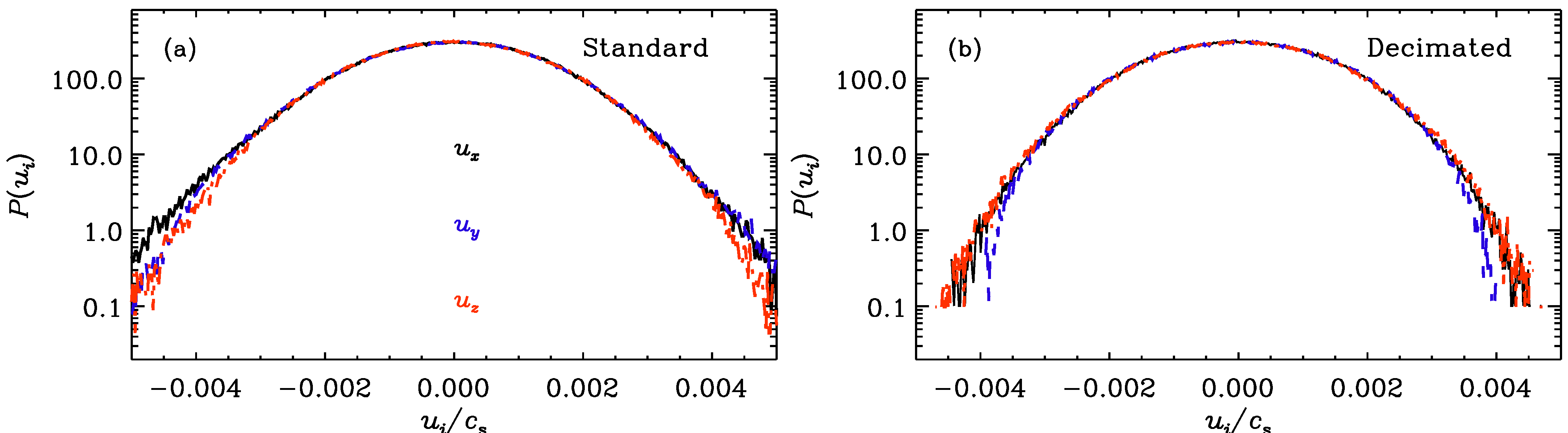
Figure 7: PDFs of all three velocity components from $64^{3}$ shearless hydrodynamic runs with $k_{\rm f}/k_{1}=5$, discussed in Appendix A. (a) standard, (b) decimated forcing with $k_{\rm min}/k_{1}=2$. All pdfs are nearly Gaussians with kurtosis $\sim 0$.

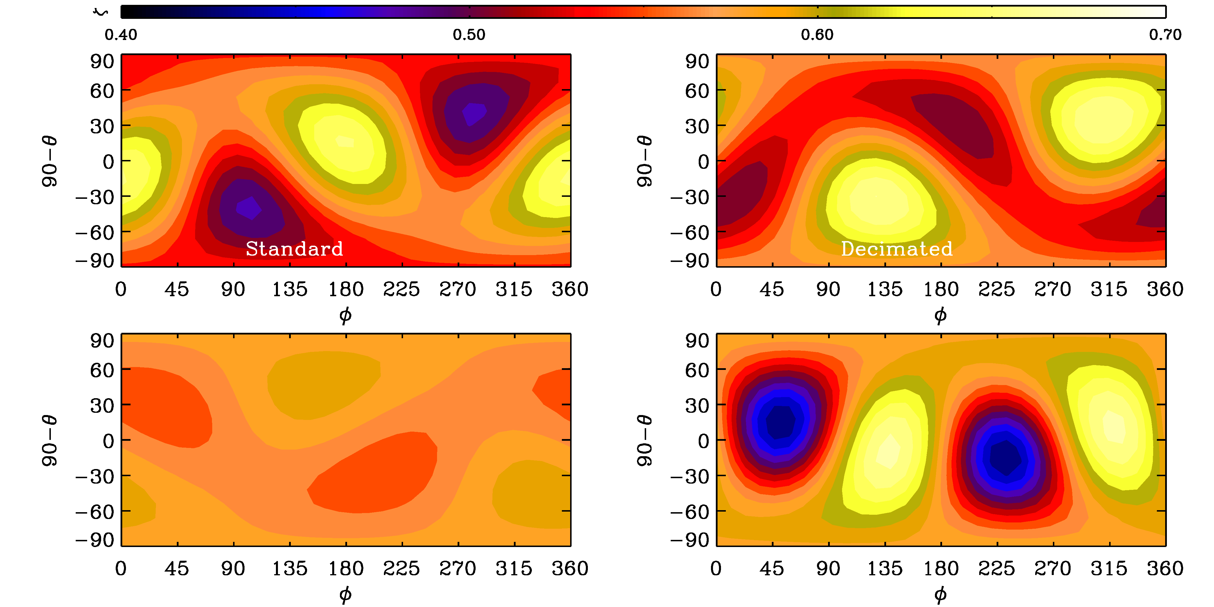
Figure 8: Distribution of $\zeta=\sqrt{\langle(\bm{u}\cdot\hat{\bm{n}})^{2}\rangle}/u_{\rm rms}$, in the $\theta\phi$ plane at times $\nu k_{\rm f}^{2}t=25$ (top) and 27.5 (bottom); from the two hydrodynamic runs discussed in Appendix A. (a) Standard; (b) decimated with $k_{\rm min}/k_{1}=2$.

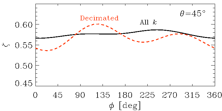
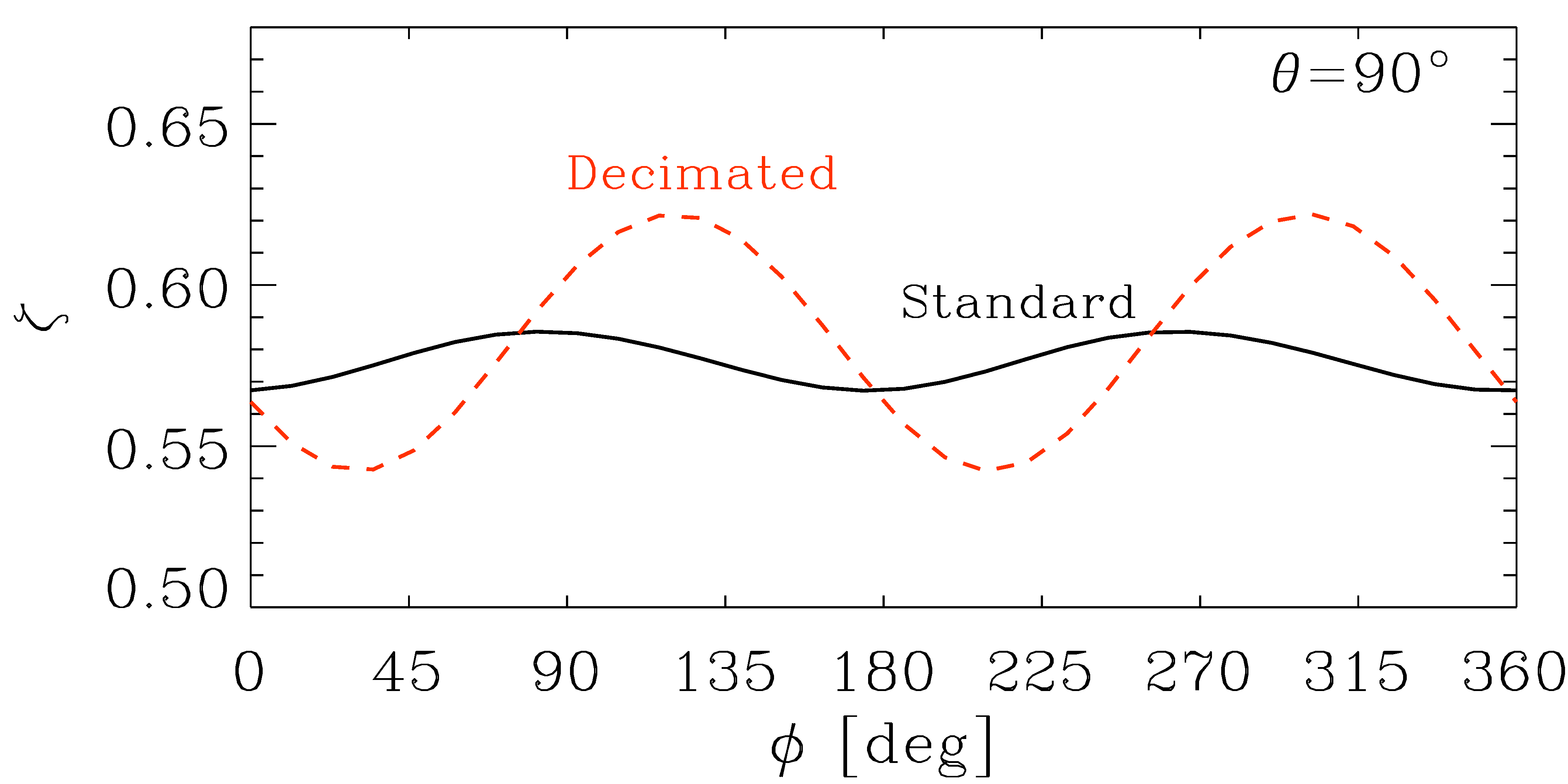
Figure 9: Variation of $\zeta$ with the azimuthal angle $\phi$ at polar angles $\theta=45\hbox{${}^{\circ}$}$ (left) and $90\hbox{${}^{\circ}$}$ (right), after averaging over eight snapshots from the runs discussed in Appendix A. Solid/black: standard; dashed/red: decimated with $k_{\rm min}/k_{1}=2$.

Appendix B Validation of the NLTFM

B.1 Comparison of the different variants of the NLTFM

Table 4: $\eta$ tensor components measured with the different variants of NLTFM from Run SKM1a007.

Method $\eta_{xx}/\eta_{0}$ $\eta_{yy}/\eta_{0}$ $\eta_{yx}/\eta_{0}$ $\eta_{xy}/\eta_{0}$ ju $2.110\pm 0.023$ $2.089\pm 0.007$ $0.112\pm 0.026$ $-0.208\pm 0.028$ jb $2.276\pm 0.152$ $2.106\pm 0.020$ $0.124\pm 0.009$ $-0.212\pm 0.018$ bb $2.297\pm 0.144$ $2.116\pm 0.018$ $0.129\pm 0.018$ $-0.188\pm 0.017$ bu $2.155\pm 0.047$ $2.127\pm 0.017$ $0.113\pm 0.014$ $-0.212\pm 0.022$

As is described in RB10, with respect to the terms $\bm{u}\times\bm{b}$ and $\bm{j}\times\bm{b}$ there are four possibilities to define the NLTFM, depending on how one combines the fluctuating fields from the main run, $\bm{u}$, $\bm{b}$, $\bm{j}$ with the test solutions $\bm{u}_{\overline{B}}$, $\bm{b}_{\overline{B}}$, $\bm{j}_{\overline{B}}$. These variants were denoted as ju (using $\bm{j}$ and $\bm{u}$ in the pondero- and electromotive forces, respectively), jb (using $\bm{j}$ and $\bm{b}$), bu (using $\bm{b}$ and $\bm{u}$), and bb (using $\bm{b}$ in both). Further variants due to the term $\bm{u}\cdot{\bm{\nabla}}\bm{u}$ are not considered here. Previously it was concluded that the ju method would be the most stable one (RB10). Here we examine how the different variants behave in SMHD with standard (random) forcing. The results for Run SKM1a007 are listed in Table LABEL:table:tfmvariants and depicted in Figure 10, showing the $\eta_{xx}$ component obtained with all four variants. We can see that jb and bb produce measurements that are nearly identical at any phase of the simulation. The measurements with bu deviate from these occasionally, but the largest deviations occur for ju. While the three former variants tend to produce turbulent transport coefficients that clearly grow within the resetting intervals, ju produces plateaus, this difference being especially pronounced in Figure 10, top panel. This is indicative of the test problems becoming unstable during the resetting interval, which can lead to overestimation of and increased uncertainties in the measured transport coefficients. With the resetting time of $0.5T_{\nu}$ in most of our simulations, however, the measured differences between the variants were very small, but nevertheless we observed a tendency of the tensor components to be larger in magnitude when jb and bb were used; see also Table LABEL:table:tfmvariants. Hence, throughout the paper we use the ju variant, which produces measurements with clearer plateaus in the turbulent transport coefficients.

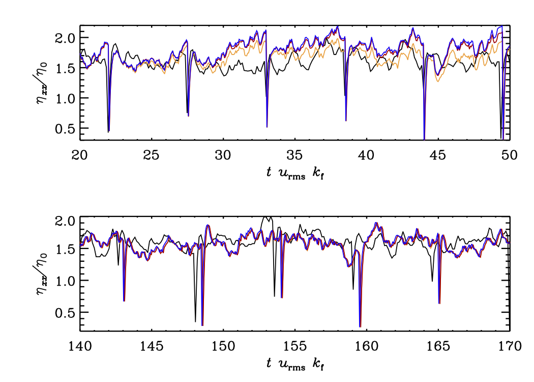
Figure 10: Time evolution of $\eta_{xx}$ from Run SKM1a007 with the four variants of the NLTFM. Black: ju, blue: bb, orange: bu, red: jb. Upper panel: early stages, lower panel: late stages of the simulation. Note that the jb results are almost completely on top of the bu ones.

B.2 Kinetically forced SMHD analyzed with QKTFM and NLTFM

To further validate the NLTFM, we perform runs of kinetically forced SMHD, and measure the turbulent transport coefficients with both QKTFM and NLTFM. We compare them in two regimes: one where the magnetic field is very weak and another where the magnetic field is already dynamically significant. We choose the setup SK4b, and show our results in Figure 11 in terms of $\eta_{yx}$ as function of time. Although some differences due to the randomness of the forcing have to be expected, we observe a very good agreement between the two methods.

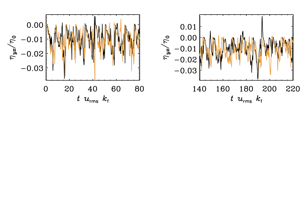
Figure 11: Time evolution of $\eta_{yx}$ from Run SK4b with QKTFM (orange) and NLTFM (black). Measurements are from a stage when the dynamo field is still weak (left) and dynamically significant (right).

Appendix C An analytical estimate for $\eta_{\it{yx}}$

To obtain an analytical estimate for $\eta_{yx}$ in the absence of the pressure term, we assume ideal MHD ($\eta=\nu=0$) and constant density, neglect terms quadratic in the fluctuations (SOCA), assume vanishing mean flow, except for $\bm{U}^{(S)}$, and vanishing initial conditions of those parts of the fluctuations which are due to the influence of shear and ${\overline{\bm{B}}}$. Then we have, restricting the mean EMF to be of first order in ${\overline{\bm{B}}}$,

$$\eta_{yx} =-\left\langle b^{(00)}_{x}(y,t)\,I_{1}-Sx\left(b^{(00)}_{x}(y,t)\,I_{2}+\int_{0}^{t}\partial_{y}b^{(00)}_{x}(\xi,\tau)d\tau\,I_{1}\right)+\,S^{2}x^{2}\int_{0}^{t}\partial_{y}b^{(00)}_{x}(\xi,\tau)d\tau\,I_{2}\right\rangle_{\!\!\!xy},$$ (C1)

$$I_{1} =\int_{0}^{t}\left(b^{(00)}_{y}(\xi,\tau)+S\int_{0}^{\tau}b^{(00)}_{x}(\xi^{\prime},\tau^{\prime})d\tau^{\prime}\right)d\tau,$$ (C2)

$$I_{2} =\int_{0}^{t}\int_{0}^{\tau}\left(\partial_{y}b^{(00)}_{y}(\xi^{\prime},\tau^{\prime})+S\int_{0}^{\tau^{\prime}}\partial_{y}b^{(00)}_{x}(\xi{{}^{\prime\prime}},\tau{{}^{\prime\prime}})d\tau{{}^{\prime\prime}}\right)d\tau^{\prime}d\tau,$$ (C3)

where $\xi=y+Sx(\tau-t)$, $\xi^{\prime}=y+Sx(\tau^{\prime}-t)$ etc. and the arguments $x$ and $z$ were dropped. The magnetic field is in units of $\rho^{1/2}$ and $\left(\bm{u}^{(00)},\bm{b}^{(00)}\right)$ is the background turbulence (i.e., for ${\overline{\bm{B}}}=\boldsymbol{0}$) without influence of shear ($S=0$), hence

$$\partial_{t}\bm{b}^{(00)} ={\bm{\nabla}}\times\left(\bm{u}^{(00)}\times\bm{b}^{(00)}\right)^{\prime}+\bm{f}_{\rm M},$$ (C4)

$$\partial_{t}\bm{u}^{(00)} =-\left(\bm{u}^{(00)}\cdot{\bm{\nabla}}\bm{u}^{(00)}-\bm{j}^{(00)}\times\bm{b}^{(00)}\right)^{\prime}+\bm{f}_{\rm K}.$$

Remarkably, there is no contribution from $\bm{u}^{(00)}$ to $\eta_{yx}$ and only $b^{(00)}_{x}\neq 0$ is necessary for $\eta_{yx}\neq 0$. To zeroth and first order in $S$ we obtain

$$\eta_{yx}= -S\left\langle b_{x}^{(00)}(y,t)\int_{0}^{t}\int_{0}^{\tau}b_{x}^{(00)}(y,\tau^{\prime})d\tau^{\prime}d\tau\right\rangle_{\!\!\!xy}-\left\langle b_{x}^{(00)}(y,t)\int_{0}^{t}b^{(00)}_{y}(y,\tau)d\tau\right\rangle_{\!\!\!xy}$$ (C5)

$$-S\left\langle xb_{x}^{(00)}(y,t)\int_{0}^{t}\partial_{y}b^{(00)}_{y}(y,\tau)(\tau-t)\,d\tau\right\rangle_{\!\!\!xy}+S\left\langle xb_{x}^{(00)}(y,t)\int_{0}^{t}\int_{0}^{\tau}\partial_{y}b^{(00)}_{y}(y,\tau^{\prime})\,d\tau^{\prime}d\tau\right\rangle_{\!\!\!xy}$$ (C6)

$$+S\left\langle x\left(\int_{0}^{t}\partial_{y}b^{(00)}_{x}(y,\tau)d\tau\right)\left(\int_{0}^{t}b^{(00)}_{y}(y,\tau)d\tau\right)\right\rangle_{\!\!\!xy},$$ (C7)

where the second contribution in (C5) vanishes in isotropic background turbulence because of $\left\langle b_{i}^{(00)}(y,t)b_{j}^{(00)}(y,\tau)\right\rangle_{\!\!xy}\propto\delta_{ij}$. Integration by parts in (C6) yields

$$\int_{0}^{t}\partial_{y}b^{(00)}_{y}(y,\tau)(\tau-t)\,d\tau=-\int_{0}^{t}\int_{0}^{\tau}\partial_{y}b^{(00)}_{y}(y,\tau^{\prime})\,d\tau^{\prime}d\tau.$$ (C8)

Further, we have

$$b_{x}^{(00)}(y,t)\int_{0}^{t}\int_{0}^{\tau}\partial_{y}b^{(00)}_{y}(y,\tau^{\prime})\,d\tau^{\prime}d\tau= \,\partial_{y}\left(b_{x}^{(00)}(y,t)\int_{0}^{t}\int_{0}^{\tau}b^{(00)}_{y}(y,\tau^{\prime})\,d\tau^{\prime}d\tau\right)$$ (C9)

$$-\partial_{y}b_{x}^{(00)}(y,t)\int_{0}^{t}\int_{0}^{\tau}b^{(00)}_{y}(y,\tau^{\prime})\,d\tau^{\prime}d\tau,$$ (C10)

in which the first term on the right vanishes under averaging over $y$. Hence, for the terms (C6) and (C7) we obtain

$$S\left\langle x\left[\left(\int_{0}^{t}\partial_{y}b^{(00)}_{x}(y,\tau)d\tau\right)\left(\int_{0}^{t}b^{(00)}_{y}(y,\tau)d\tau\right)-2\,\partial_{y}b_{x}^{(00)}(y,t)\int_{0}^{t}\int_{0}^{\tau}b^{(00)}_{y}(y,\tau^{\prime})\,d\tau^{\prime}d\tau\right]\right\rangle_{\!\!\!xy}.$$ (C11)

Because of isotropy and mirror symmetry of the background turbulence, the correlator $\left\langle b_{i}^{(00)}(y,t)\partial_{k}b^{(00)}_{j}(y,\tau)\right\rangle_{\!\!xy}$ vanishes $\forall i,j$. Hence, it is only the factor $x$ in (C11) that possibly prevents this term from vanishing, in contrast to the first term in (C5), which is based on a correlator, usually assumed positive definite.

On the other hand, truly Galilean-invariant turbulence should not exhibit an explicit $x$ dependence. Given that the forcing in our simulations indeed obeys Galilean invariance, deviations from it in $\bm{u}$ and $\bm{b}$ can only emerge due to the “memory” of the turbulence, which is made “everlasting” by the absence of dissipative damping. Thus, for the purpose of interpreting our numerical results, we may disregard (C11) and assume that only the first term in (C5) determines the sign of $\eta_{yx}$.

Comparing with Squire & Bhattacharjee (2015a) by setting $\nu=\eta=0$ in their Equations (32)–(35) we find the following agreements:

• no contribution from $\bm{u}^{(00)}$ (or $W_{u}$ in their terms) to $\eta_{yx}$, only from $\bm{b}^{(00)}$ (or $W_{b}$),

• $\eta_{yx}$ has the opposite sign of $S$ and is thus unfavorable for the MSC-effect dynamo
  (for this we have to assume a positive correlation $\left\langle b_{x}^{(00)}(y,t;x,z)\,b_{x}^{(00)}(y,\tau^{\prime};x,z)\right\rangle_{\!\!xy}$).

In summary, our analytical result is in qualitative accordance with the numerical ones for the magneto-kinetic forcing cases. For the purely kinetic ones, however, the analytics predicts vanishing $\eta_{yx}$, while the numerical experiments do produce it, even with a favorable sign for dynamo action, albeit too weak to be its main driver, and also weaker than in comparable magneto-kinetic forcing setups. As vanishing $\eta_{yx}$ is in agreement with the ideal limit of Squire & Bhattacharjee (2015a), we conclude that a nonzero contribution to $\eta_{yx}$ from kinetic fluctuations and shear (their $(\eta_{yx})_{u}^{S}$), requires the presence of dissipative terms, most likely $\eta\neq 0$, as their result (32) suggests. It also reveals that there must be an “optimal” magnitude of $\eta$ that maximizes $\left|(\eta_{yx})_{u}^{S}\right|$ because it vanishes again in the limit $\eta\rightarrow\infty$. To be too far from the optimal $\eta$ in numerical setups might explain the absence of a dynamo, enabled by $(\eta_{yx})_{u}^{S}$.

References

- Blackman (2010) Blackman, E. G. 2010, AN, 331, 101, doi: 10.1002/asna.200911304
- Blackman & Field (2001) Blackman, E. G., & Field, G. B. 2001, Physics of Plasmas, 8, 2407, doi: 10.1063/1.1351830
- Brandenburg (2001) Brandenburg, A. 2001, ApJ, 550, 824, doi: 10.1086/319783
- Brandenburg et al. (1995) Brandenburg, A., Nordlund, A., Stein, R. F., & Torkelsson, U. 1995, ApJ, 446, 741, doi: 10.1086/175831
- Brandenburg et al. (2008) Brandenburg, A., Rädler, K. H., Rheinhardt, M., & Käpylä, P. J. 2008, ApJ, 676, 740, doi: 10.1086/527373
- Brandenburg et al. (2012) Brandenburg, A., Sokoloff, D., & Subramanian, K. 2012, Space Sci. Rev., 169, 123, doi: 10.1007/s11214-012-9909-x
- Brandenburg & Subramanian (2005) Brandenburg, A., & Subramanian, K. 2005, Phys. Rep., 417, 1, doi: 10.1016/j.physrep.2005.06.005
- Brandenburg et al. (2020) Brandenburg, A., Johansen, A., Bourdin, P. A., et al. 2020, arXiv e-prints, arXiv:2009.08231. https://arxiv.org/abs/2009.08231
- Cattaneo & Vainshtein (1991) Cattaneo, F., & Vainshtein, S. I. 1991, ApJ, 376, L21, doi: 10.1086/186093
- Chamandy & Singh (2018) Chamandy, L., & Singh, N. K. 2018, MNRAS, 481, 1300, doi: 10.1093/mnras/sty2301
- Devlen et al. (2013) Devlen, E., Brandenburg, A., & Mitra, D. 2013, MNRAS, 432, 1651, doi: 10.1093/mnras/stt590
- Elperin et al. (2003) Elperin, T., Kleeorin, N., & Rogachevskii, I. 2003, PhRvE, 68, 016311, doi: 10.1103/PhysRevE.68.016311
- Frisch & Bec (2001) Frisch, U., & Bec, J. 2001, in New trends in turbulence. Turbulence: nouveaux aspects, Les Houches Session LXXIV 31 July - 1 September 2000, ed. M. Lesieur, A.Yaglom and F. David, Vol. 74 (Springer EDP-Sciences), 341–383, doi: 10.1007/3-540-45674-0
- Haugen et al. (2004) Haugen, N. E. L., Brandenburg, A., & Mee, A. J. 2004, MNRAS, 353, 947, doi: 10.1111/j.1365-2966.2004.08127.x
- Heinemann et al. (2011) Heinemann, T., McWilliams, J. C., & Schekochihin, A. A. 2011, Phys. Rev. Lett., 107, 255004, doi: 10.1103/PhysRevLett.107.255004
- Hubbard et al. (2009) Hubbard, A., Del Sordo, F., Käpylä, P. J., & Brandenburg, A. 2009, MNRAS, 398, 1891, doi: 10.1111/j.1365-2966.2009.15108.x
- Käpylä et al. (2009) Käpylä, P. J., Mitra, D., & Brandenburg, A. 2009, PhRvE, 79, 016302, doi: 10.1103/PhysRevE.79.016302
- Käpylä et al. (2020) Käpylä, P. J., Rheinhardt, M., Brandenburg, A., & Käpylä, M. J. 2020, A&A, 636, A93, doi: 10.1051/0004-6361/201935012
- Lanotte et al. (1999) Lanotte, A., Noullez, A., Vergassola, M., & Wirth, A. 1999, Geophysical and Astrophysical Fluid Dynamics, 91, 131, doi: 10.1080/03091929908203701
- Lesur & Ogilvie (2008) Lesur, G., & Ogilvie, G. I. 2008, A&A, 488, 451, doi: 10.1051/0004-6361:200810152
- Marston et al. (2008) Marston, J. B., Conover, E., & Schneider, T. 2008, Journal of Atmospheric Sciences, 65, 1955, doi: 10.1175/2007JAS2510.1
- Mitra & Brandenburg (2012) Mitra, D., & Brandenburg, A. 2012, MNRAS, 420, 2170, doi: 10.1111/j.1365-2966.2011.20190.x
- Pipin & Seehafer (2009) Pipin, V. V., & Seehafer, N. 2009, A&A, 493, 819, doi: 10.1051/0004-6361:200810766
- Rädler (1969a) Rädler, K. H. 1969a, Monats. Dt. Akad. Wiss., 11, 194
- Rädler (1969b) —. 1969b, Monats. Dt. Akad. Wiss., 11, 272
- Rheinhardt & Brandenburg (2010) Rheinhardt, M., & Brandenburg, A. 2010, A&A, 520, A28, doi: 10.1051/0004-6361/201014700
- Rheinhardt & Brandenburg (2012) —. 2012, Astronomische Nachrichten, 333, 71, doi: 10.1002/asna.201111625
- Rogachevskii & Kleeorin (2003) Rogachevskii, I., & Kleeorin, N. 2003, PhRvE, 68, 036301, doi: 10.1103/PhysRevE.68.036301
- Rogachevskii & Kleeorin (2004) —. 2004, PhRvE, 70, 046310, doi: 10.1103/PhysRevE.70.046310
- Schrinner et al. (2005) Schrinner, M., Rädler, K.-H., Schmitt, D., Rheinhardt, M., & Christensen, U. 2005, Astron. Nachr., 326, 245, doi: 10.1002/asna.200410384
- Schrinner et al. (2007) Schrinner, M., Rädler, K.-H., Schmitt, D., Rheinhardt, M., & Christensen, U. R. 2007, Geophysical and Astrophysical Fluid Dynamics, 101, 81, doi: 10.1080/03091920701345707
- Shi et al. (2016) Shi, J.-M., Stone, J. M., & Huang, C. X. 2016, MNRAS, 456, 2273, doi: 10.1093/mnras/stv2815
- Singh & Jingade (2015) Singh, N. K., & Jingade, N. 2015, ApJ, 806, 118, doi: 10.1088/0004-637X/806/1/118
- Singh & Sridhar (2011) Singh, N. K., & Sridhar, S. 2011, PhRvE, 83, 056309, doi: 10.1103/PhysRevE.83.056309
- Squire & Bhattacharjee (2015a) Squire, J., & Bhattacharjee, A. 2015a, PhRvE, 92, 053101, doi: 10.1103/PhysRevE.92.053101
- Squire & Bhattacharjee (2015b) —. 2015b, ApJ, 813, 52, doi: 10.1088/0004-637X/813/1/52
- Squire & Bhattacharjee (2016) —. 2016, J. Plasma Phys., 82, 535820201, doi: 10.1017/S0022377816000258
- Sridhar & Singh (2010) Sridhar, S., & Singh, N. K. 2010, J. Fluid Mech., 664, 265, doi: 10.1017/S0022112010003745
- Sridhar & Singh (2014) —. 2014, MNRAS, 445, 3770, doi: 10.1093/mnras/stu1981
- Sridhar & Subramanian (2009a) Sridhar, S., & Subramanian, K. 2009a, PhRvE, 79, 045305, doi: 10.1103/PhysRevE.79.045305
- Sridhar & Subramanian (2009b) —. 2009b, PhRvE, 80, 066315, doi: 10.1103/PhysRevE.80.066315
- Vainshtein & Cattaneo (1992) Vainshtein, S. I., & Cattaneo, F. 1992, ApJ, 393, 165, doi: 10.1086/171494
- Yousef et al. (2008a) Yousef, T. A., Heinemann, T., Rincon, F., et al. 2008a, Astron. Nachr., 329, 737, doi: 10.1002/asna.200811018
- Yousef et al. (2008b) Yousef, T. A., Heinemann, T., Schekochihin, A. A., et al. 2008b, Phys. Rev. Lett., 100, 184501, doi: 10.1103/PhysRevLett.100.184501