Why Attentions May Not Be Interpretable?

Abstract.

Attention-based methods have played important roles in model interpretations, where the calculated attention weights are expected to highlight the critical parts of inputs (e.g., keywords in sentences). However, recent research found that attention-as-importance interpretations often do not work as we expected. For example, learned attention weights sometimes highlight less meaningful tokens like “[SEP]”, “,”, and “.”, and are frequently uncorrelated with other feature importance indicators like gradient-based measures. A recent debate over whether attention is an explanation or not has drawn considerable interest. In this paper, we demonstrate that one root cause of this phenomenon is the combinatorial shortcuts, which means that, in addition to the highlighted parts, the attention weights themselves may carry extra information that could be utilized by downstream models after attention layers. As a result, the attention weights are no longer pure importance indicators. We theoretically analyze combinatorial shortcuts, design one intuitive experiment to show their existence, and propose two methods to mitigate this issue. We conduct empirical studies on attention-based interpretation models. The results show that the proposed methods can effectively improve the interpretability of attention mechanisms.

1. Introduction

Interpretation for machine learning models has gained increasing interest and becomes necessary in practice as the industry rapidly embraces machine learning technologies. Model interpretation explains how models make decisions, which is particularly essential in mission-critical domains where the accountability and transparency of the decision-making process are crucial, such as medicine (Wang et al., 2019), security (Chakraborti et al., 2019), and criminal justice (Lipton, 2018).

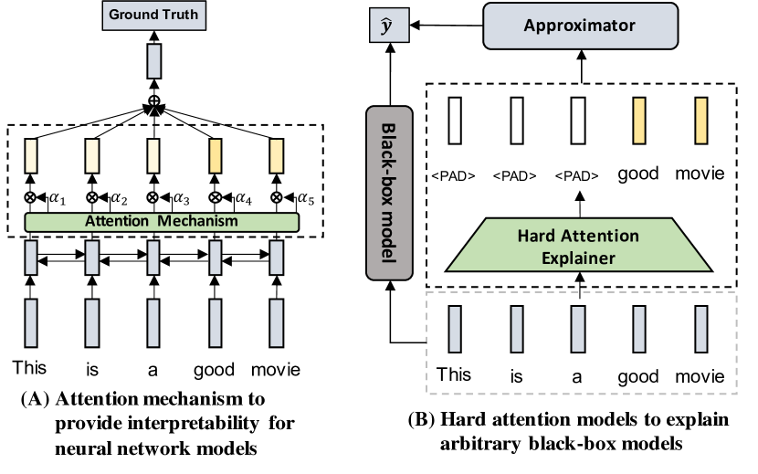
Figure 1. The use of attention for model interpretations. With specific architectures, attention mechanisms can both provide interpretability for neural networks, and select features to explain black-box models.

Attention mechanisms have played important roles in model interpretations. As shown in Figure 1, attention mechanism as building blocks in neural networks are often applied to provide interpretability along with improving performance (Choi et al., 2016; Vaswani et al., 2017; Wang et al., 2016), and hard attention-based models are also used in explaining arbitrary black-box models’ predictions, by selecting a fixed number of input components to approximate the predictions (Chen et al., 2018; Liang et al., 2020; Belinkov and Glass, 2019). More concretely, we formalize the attention mechanisms as $\text{Attention}(Q,K,V)=\text{Mask}(Q,K)\odot V$ as in (Vaswani et al., 2017), where $Q$ is the query and $\langle K,V\rangle$ are the key-value pairs. $\text{Mask}(\cdot,\cdot)$ maps the query and keys to the attention weights (denoted as masks in this paper), and then the masks filter the information of $V$. In other words, the masks are expected to represent the importance of different parts of $V$ (e.g., words of a sentence, pixels of an image) and highlight those the models focus on to make decisions.

However, recent research suggested that the feature parts highlighted by attention mechanisms do not necessarily correlate with intuitively greater importance on the final predictions. For example, Clark et al. (2019) found that a surprisingly large amount of BERT’s attention focuses on less meaningful tokens like “[SEP]”, “,”, and “.”. Moreover, many researchers have provided evidence to support or refute the interpretability of the attention mechanisms. There have been lots of debates on whether attention is an explanation or not recently (Jain and Wallace, 2019; Serrano and Smith, 2019; Wiegreffe and Pinter, 2019).

In this paper, we propose that a root cause hindering the interpretability of attention mechanisms is combinatorial shortcuts. As mentioned earlier, we expect that the results of attention mechanisms mainly contain information from the highlighted parts of $V$, which is a critical assumption for attention-based interpretations’ effectiveness. However, as the results are products of the masks and $V$, we find that the masks themselves can carry extra information other than the highlighted parts of $V$, which the downstream parts of models could utilize. As a result, the calculated masks may work as another kind of “encoding layers” rather than providing pure feature importance. For an extreme example, in a (binary) text classification task, the attention mechanisms could highlight the first word for positive cases and highlight the last one for negative cases, regardless of the word semantics. The downstream parts of attention layers can then predict the label by checking whether the first or the last word is highlighted, which may give good accuracy scores but completely fail to provide interpretability.

We further study the effectiveness of attention-based interpretations and dive into the combinatorial shortcut problem. From the perspective of causal effect estimations, we first analyze the difference between coventional attention mechanisms and ideal interpretations theoretically, and then show the existence of combinatorial shortcuts through a constructive experiment. Based on the observations, we propose two methods to mitigate the issue, i.e., random attention pretraining and instance weighting for mask-neutral learning. Without loss of generality, we examine the effectiveness of the proposed methods with an end-to-end attention-based model-interpretation approach, i.e., L2X (Chen et al., 2018), which can select a given number of input components to explain arbitrary black-box models. Experimental results show that the proposed methods can successfully mitigate the adverse impact of combinatorial shortcuts and improve explanation performance.

2. Related Work

Attention mechanisms for model interpretations  Attention mechanisms have been widely adopted in natural language processing (Bahdanau et al., 2015; Vinyals et al., 2015), computer vision (Fu et al., 2016; Li et al., 2019), recommendations (Bai et al., 2020; Zhang et al., 2020a) and so on. Attention mechanisms have been used to explain how models make decisions by exhibiting the importance distribution over inputs (Choi et al., 2016; Martins and Astudillo, 2016; Wang et al., 2016), which we can regard as a kind of model-specific interpretation. Besides, there are also attention-based methods for model-agnostic interpretations. For example, L2X (Chen et al., 2018) is a hard attention model (Xu et al., 2015) that employs Gumbel-softmax (Jang et al., 2017) for instancewise feature selection. VIBI (Bang et al., 2019) improved L2X to encourage the briefness of the learned explanation by adding a constraint for the feature scores to a global prior. Liang et al. (2020) and Yu et al. (2019) improved attention-style model interpretation methods through adversarial training to encourage the gap between the predictability of selected/unselected features.

However, there has been a debate on the interpretability of attention mechanisms recently. Jain and Wallace (2019) suggested that “attention is not explanation” by finding that the attention weights are frequently uncorrelated with other feature importance indicators like gradient-based measures. On the other side, Wiegreffe and Pinter (2019) argued that “attention is not not-explanation” by challenging many assumptions underlying Jain and Wallace (2019) and suggested that they did not disprove the usefulness of attention mechanisms for explainability. Serrano and Smith (2019) applied a different analysis based on intermediate representation erasure and found that while attention noisily predicts input components’ overall importance to a model, it is by no means a fail-safe indicator.

In this work, we take another perspective on this problem called combinatorial shortcuts, and show that it can provide one root cause of the phenomenon. We analyze why combinatorial shortcuts exist and propose theoretically guaranteed methods to alleviate the problem.

Causal effect estimations  Causal effect is an important concept for quantitative empirical analyses. The causal effect of one treatment, $E$, over another, $C$, is defined as the difference between what would have happened if a particular unit had been exposed to $E$ and what would have happened if the unit had been exposed to $C$ (Rubin, 1974). Randomized experiments, where the experimental units across the treatment groups are randomly allocated, play a critical role in causal inference. However, when randomized experiments are infeasible, researchers have to resort to nonrandomized data from surveys, censuses, and administrative records (Winship and Morgan, 1999), and there may be some other variables controlling the treatment allocation process in such data. For example, consider the causal inference between uranium mining and health. Ideally, the treatment (uranium mining) should be randomly allocated. However, mining workers are usually stronger people among all humans in the world. If some appropriate measures are absent, we may draw biased conclusions like “uranium mining has no adverse health impact because the average life span of uranium mine workers is not shorter than that of ordinary people”. For recovering causal effects from nonrandomized data, instance weighting-based approaches have been used widely (Ertefaie and Stephens, 2010; Rosenbaum and Rubin, 1983; Winship and Morgan, 1999).

3. Combinatorial Shortcuts

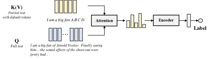
Figure 2. The structure of the model used in this demo experiment. The attention is restricted to the first five tokens of sentences and four default tokens that appear in all samples. After the Attention module, the weighted sequences are further encoded to a fixed-length vector with the Encoder module.

Table 1. Experiments about how much attention is put to default tokens out of all attention weights. Both Pooling and RCNN are tested as the Encoder module in Figure 2. Note that we report the results on the training set to demonstrate how models fit the data.

No.	Encoder	Label	Attention to default tokens
			A	B	C	D	Total
(1)	Pooling	pos	68.0%	0.1%	0.0%	0.2%	68.3%
(2)		neg	0.1%	36.6%	38.3%	18.5%	93.5%
(3)	RCNN	pos	16.1%	0.2%	0.1%	0.6%	17.0%
(4)		neg	1.3%	20.2%	50.4%	13.3%	85.2%

In this section, by showing the difference between attention mechanisms and ideal explanations, we analyze why attention mechanisms become less interpretable from the perspective of causal effect estimations, and conduct an experiment to demonstrate the existence of combinatorial shortcuts.

3.1. The difference between attention mechanisms and ideal explanations

Firstly, we analyze what ideal explanations are. Although the concept of “explanation” may differ in different situations, following the idea of “finding the most dominating feature components”, we define the ideal explanations as follows in this paper. We use uppercase letters to represent random variables, and lowercase letters to represent specific values of random variables. Assume that we have samples drawn independently and identically distributed (i.i.d.) from a distribution with domain $\mathcal{X}\times\mathcal{Y}$, where $\mathcal{X}$ is the feature domain, and $\mathcal{Y}$ is the label domain. Additionally, we assume that the mask is drawn from a distribution with domain $\mathcal{M}$. Usually, $\mathcal{M}$ is under some constraints for briefness, for example, only being able to select a fixed number of features or being non-negative and summing to $1$. Given any sample $\langle x,y\rangle\sim\mathcal{X}\times\mathcal{Y}$, for $m_{1}\sim\mathcal{M}$ and $m_{2}\sim\mathcal{M}$, if $\mathcal{L}\big{(}\mathbb{E}(Y|x\odot m_{1}),y\big{)}<\mathcal{L}\big{(}\mathbb{E}(Y|x\odot m_{2}),y\big{)}$ where $\mathcal{L}(\cdot)$ is the loss function and $\mathbb{E}(\cdot)$ calculates the expectation, we say that for this sample, $m_{1}$ is superior to $m_{2}$ in term of interpretability. If an unbiased estimation of $\mathbb{E}(Y|X\odot M)$ is available, the best mask for sample $\langle x,y\rangle$ that can select the most informative features can be obtained by solving $\operatorname*{argmin}_{m}\mathcal{L}\big{(}\mathbb{E}(Y|x\odot m),y\big{)}$. As a conclusion, under the definitions above, the ideal explanation $m^{*}$ for sample $\langle x,y\rangle$ is $\operatorname*{argmin}_{m}\mathcal{L}\big{(}\mathbb{E}(Y|x\odot m),y\big{)}$ with an unbiased estimation of $\mathbb{E}(Y|X\odot M)$.

In practice, we often need to train models to estimate $\mathbb{E}(Y|X\odot M)$. Ideally, if the data (combinations of $X$ and $M$, as well as the label $Y$) is exhaustive and the model is consistent, we can train a model to obtain an unbiased estimation of $\mathbb{E}(Y|X\odot M)$ following the empirical risk minimization principle (Fan et al., 2005; Vapnik, 1992). Nevertheless, it is impossible to exhaust all combinations of $X$ and $M$. Taking a step back, from the perspective of causal effect estimations, we could consider different $M$ as different treatment, and randomized combinations for $X$ and $M$ can still be proven to give unbiased estimations on expectations (Rubin, 1974).

However, attention mechanisms do not work in this way. Considering the downstream part of attention models, i.e., the part estimating the function $\mathbb{E}(Y|X\odot M)$, we can find that it receives highly selective combinations of $X$ and $M$. The used mask $M$ during the training procedure is a mapping from query and keys, making the used mask for samples highly related to the feature $X$ (and $Y$ as well). Consequently, the training procedure of the attention mechanism produces a nonrandomized experiment (Shadish et al., 2008). Therefore the model cannot learn unbiased $\mathbb{E}(Y|X\odot M)$. In turn, the attention mechanism will try to select biased features to adapt the biased estimations to minimize the overall loss functions, and thus fail to highlight the essential features. As a result, the attention mechanism and downstream part may cooperate and find unexpected ways to fit the data, e.g., highlighting the first word for positive cases and the last word for negative cases, ultimately failing to provide interpretability. This paper denotes the effects of nonrandomized combination for $X$ and $M$ that hinders the interpretability of attention mechanisms as combinatorial shortcuts.

3.2. Experimental demonstration for the combinatorial shortcuts

To intuitively demonstrate the existence of combinatorial shortcuts, we design a simple experiment on text classification tasks. As Figure 2 shows, we train attention models, where the query of attention is encoded with the whole sentences. However, we only allow attention to highlight keywords among the first five tokens and four default tokens, i.e., “A”, “B”, “C”, and “D”. After the Attention module, the weighted sequences are further encoded to a fixed-length vector with the Encoder module, and finally to predict the labels. Since the default tokens appear in all samples and do not carry any meaningful information, if the attention mechanism can highlight the inputs’ critical parts, little attention should be paid to them. Moreover, we could check whether the models put differential attention to default tokens for different classes to show if the information is encoded in the mask due to combinatorial shortcuts.

We use the real-world IMDB dataset (Maas et al., 2011) for experiments and examine different settings regarding the Encoder module in Figure 2, i.e., whether the encoder is a simple sum pooling or a position-aware trainable neural network model, i.e., recurrent convolutional neural network (RCNN) proposed by Lai et al. (2015). We use pre-trained GloVe word embeddings (Pennington et al., 2014) and keep them fixed to prevent shortcuts through word embeddings. We train soft attention models for 25 epochs with RMSprop optimizers using default parameters and record the averaged results of 10 runs. The results are reported in Table 1.

As we can see in Table 1, the attention models placed more than half of the attention weights to the default tokens, and the weights for different classes were significantly different. Taking Pooling encoders as an example, the models put up to 68.0% attention weights to default token “A” for positive samples, and put 36.6%, 38.3%, and 18.5% attention weights to default token “B”, “C”, and “D” respectively for negative samples, summing up to 93.4% in total. As for RCNN encoders, the results were similar. The reason for observing repeatable results on default tokens with different initialization may be due to their slight asymmetry in the GloVe embedding space, i.e., “A” is slightly closer to “good” than to “bad”, while the other three default tokens are just the opposite. These results suggest that the attention mechanism may not work as expected to highlight the critical parts of inputs and provide interpretability. Instead, they learn to work as another kind of “encoding layers” and utilize the default tokens to fit the data through combinatorial shortcuts.

4. Methods for Mitigating Combinatorial Shortcuts

In this section, based on the perspective of causal effect estimations introduced in Section 3.1, we come up with two methods, random attention pretraining and mask-neutral learning with instance weighting respectively, to mitigate combinatorial shortcuts for better interpretability. Then we compare the pros and cons of the two methods.

4.1. Random attention pretraining

We first propose a simple and straightforward method to address the issue. As analyzed in Section 3.1, the fundamental reason for combinatorial shortcuts is the biased estimation of $\mathbb{E}(Y|X\odot M)$, and random combinations of $X$ and $M$ can give unbiased results in theory.

Inspired by this idea, we can generate the masks completely at random and train the attention model’s downstream part. We then fix the downstream part, replace the random attention with a trainable attention layer, and train the attention layer only. As the downstream parts of neural networks are trained unbiasedly and fixed, solely training the attention layers is solving $m^{*}=\operatorname*{argmin}_{m}\mathcal{L}\big{(}\mathbb{E}(Y|x\odot m),y\big{)}$ with an unbiased estimation of $\mathbb{E}(Y|X\odot M)$. Thus the interpretability is guaranteed.

4.2. Mask-neutral learning with instance weighting

The second method is based on instance weighting, which has been successfully applied for mitigating sample selection bias (Zadrozny, 2004; Zhang et al., 2019), social prejudices bias (Zhang et al., 2020b), and also for recovering the causal effects (Ertefaie and Stephens, 2010; Winship and Morgan, 1999). The core idea of this method is that instead of fitting a biased $\mathbb{E}(Y|X\odot M)$, with instance weighting, we could recover a mask-neutral distribution where the masks are unrelated to the labels. Thus the downstream parts of attention layers become less biased, and combinatorial shortcuts can be partially mitigated.

Assumptions about the biased distribution and the mask-neutral distribution  We first define the mask-neutral distribution and its relationship with the biased distribution with which ordinary attention mechanisms are trained. Considering the downstream part of the attention layers, which estimates $\mathbb{E}(Y|X\odot M)$, we assume that there is a mask-neutral distribution $\mathscr{Q}$ with domain $\mathcal{X}\times\mathcal{Y}\times\mathcal{M}\times\mathcal{S}$, where $\mathcal{X}$ is the feature space, $\mathcal{Y}$ is the (binary) label space, $\mathcal{M}$ is the feature mask space, and $\mathcal{S}$ is the binary sampling indicator space. During the training procedure, the selective combination of masks and features result in combinatorial shortcuts. We assume for any given sample $(x,y,m,s)$ drawn independently from $\mathscr{Q}$, it will be selected to appear in the training of attention mechanisms if and only if $s=1$, which results in the biased distribution $\mathscr{P}$. We use $P(\cdot)$ to represent probabilities of the biased distribution $\mathscr{P}$, and $Q(\cdot)$ for the mask-neutral distribution $\mathscr{Q}$, then we have

(1) $$P(\cdot)=Q(\cdot|S=1)\,.$$

Ideally, we should have $M\perp(X,Y)$ on $\mathscr{Q}$ to obtain unbiased $\mathbb{E}(Y|X\odot M)$ as discussed in Section 3.1. However, when both sides are vectors, it will be intractable. Therefore, we take a step back and only assume $Y\perp M$ on $\mathscr{Q}$, i.e.,

(2) $$Q(Y|M)=Q(Y)\,.$$

If $S$ is completely at random, $\mathscr{P}$ will be consistent with $\mathscr{Q}$. However, the attention layers are highly selective, making that only some combinations of $X$ and $M$ are visible to the downstream model. We assume that $M$ and $Y$ control $S$. And for any given $Y$ and $M$, the probability of selection is greater than $0$, defined as

(3) $$Q(S=1|X,Y,M)=Q(S=1|Y,M)>0\,.$$

To further simplify the problem, we assume that the selection does not change the marginal probability of $M$ and $Y$, i.e.,

(4) $$P(M)=Q(M)\,,P(Y)=Q(Y)\,.$$

In other words, we assume that although $S$ is dependent on the combination of $M$ and $Y$ in $\mathscr{Q}$, it is independent on either $M$ or $Y$ only, i.e., $Q(S|M)=Q(S)$ and $Q(S|Y)=Q(S)$.

The unbiased expectation of loss with instance weighting  We show that, by adding proper instance weights, we can obtain an unbiased estimation of the loss on the mask-neutral distribution $\mathscr{Q}$, with only the data from the biased distribution $\mathscr{P}$.

Fact 1 (Unbiased Loss Expectation).

For any function $f=f(x\odot m)$, and for any loss $\mathcal{L}=\mathcal{L}\big{(}f(x\odot m),y\big{)}$, if we use $w=\frac{P(y)}{P(y|m)}$ as the instance weights, then

Fact 1 shows that, by a proper instance-weighting method, the downstream part of the attention model can learn on the mask-neutral distribution $\mathscr{Q}$, where $Q(Y|M)=Q(Y)$. Therefore, the independence between $M$ and $Y$ is encouraged, then it will be hard for the classifier to approximate $Y$ solely by $M$. Thus, the classifier will have to use useful information from $X$, and have the combinatorial shortcuts problem mitigated.

We present the proof for Fact 1 as follows.

Proof.

We first present an equation with the weight $w$,

$$\begin{split}w=&\frac{P(y)}{P(y|m)}=\frac{Q(y)}{Q(y|m,S=1)}\\ =&\frac{Q(y)}{Q(S=1|y,m)Q(y|m)/Q(S=1|m)}\\ =&\frac{Q(S=1)}{Q(S=1|y,m)}\\ =&\frac{Q(S=1)}{Q(x,y,m|S=1)Q(S=1)/Q(x,y,m)}\\ =&\frac{Q(x,y,m)}{P(x,y,m)}\,\text{.}\end{split}$$

Then we have

$$\begin{split}&\mathbb{E}_{x,y,m\sim\mathscr{P}}\Big{[}w\mathcal{L}\big{(}f(x\odot m),y\big{)}\Big{]}\\ =&\int\frac{Q(x,y,m)}{P(x,y,m)}\mathcal{L}\big{(}f(x\odot m),y\big{)}dP(x,y,m)\\ =&\int\mathcal{L}\big{(}f(x\odot m),y\big{)}dQ(x,y,m)\\ =&\mathbb{E}_{x,y,m\sim\mathscr{Q}}\Big{[}\mathcal{L}\big{(}f(x\odot m),y\big{)}\Big{]}\,.\end{split}$$

∎

Mask-neutral learning  With Fact 1, we now propose mask-neutral learning for better interpretability of attention mechanisms. As shown, by adding instance weight $w=\frac{P(y)}{P(y|m)}$ to the loss function, we can obtain unbiased loss of the mask-neutral distribution. As distribution $\mathscr{P}$ is directly observable, estimating $P(\cdot)$ is possible. In practice, we could train a classifier to estimate $P(Y|M)$ along with the training of the attention layer, optimize it and the attention layers, as well as the other parts of models alternatively.

Table 2. Effectiveness of the proposed methods for mitigating the combinatorial shortcuts.

No.	Method	Encoder	Label	Attention to default tokens
				A	B	C	D	Total
(1)	Pretraining	Pooling	pos	0.0%	4.6%	2.3%	0.0%	6.9%
(2)			neg	0.0%	0.4%	20.2%	0.0%	20.6%
(3)		RCNN	pos	0.2%	1.1%	1.0%	0.3%	2.6%
(4)			neg	2.3%	4.3%	6.3%	2.8%	15.7%
(5)	Weighting	Pooling	pos	1.3%	2.5%	0.5%	2.2%	6.5%
(6)			neg	3.3%	0.7%	1.5%	1.2%	6.7%
(7)		RCNN	pos	6.7%	1.4%	10.3%	2.1%	20.5%
(8)			neg	4.6%	1.8%	12.5%	1.9%	20.8%

4.3. Comparison of the two methods

As analyzed in Section 3.1, random attention pretraining is complete in theory. However, it may be practically incompetent because there are countless viable cases of the combinations of $X$ and $M$. It could be challenging to estimate $\mathbb{E}(Y|X\odot M)$ well, especially when the dimension of input features is high or strong co-adapting patterns exist in the data. Under such cases, the pretraining procedure may become less efficient as it needs to explore all possible masks evenly, even if most of the masks are worthless. In conclusion, the model may fail to estimate complex $\mathbb{E}(Y|X\odot M)$ functions well in some cases, which finally limits the interpretability.

Compared with the random attention pretraining method, the instance weighting-based approach concentrates more on the useful masks to address the shortcomings. Thus it will suffer less from the efficiency problem. Nevertheless, the effectiveness of the instance weighting method relies on the assumptions as shown in Equation (1)–(4). However, in some cases, the assumptions may not hold. For example, in Equation (3), we assume that given $Y$ and $M$, $S$ is independent on $X$. In other words, $X$ controls $S$ only through $Y$. This assumption is necessary for simplifying the problem, but may not sometimes hold when given $Y$ and $M$, $X$ can still influence $S$. Besides, the effectiveness of the method also relies on an accurate estimation of $P(Y|M)$, which may require careful tuning as the probability $P(Y|M)$ is dynamically changing along the training process of attention mechanisms.

5. Experiments

In this section, we present the experimental results of the proposed methods. For simplicity, we denote random attention pretraining as Pretraining and mask-neutral learning with instance weighting as Weighting. Firstly, we analyze the effectiveness of mitigating combinatorial shortcuts. Then, we examine the effectiveness of improving interpretability.

5.1. Experiments for mitigating combinatorial shortcuts

We applied the proposed methods to the experiments introduced in Section 3.2 to check whether we can mitigate the combinatorial shortcuts. We summarize the results in Table 2.

As presented, after applying Pretraining and Weighting, the percentage of attention weights assigned to the default tokens were significantly reduced. Since that the default tokens do not provide useful information but only serve as carriers for combinatorial shortcuts, the results reveal that our methods have mitigated the combinatorial shortcuts successfully.

5.2. Experiments for improving interpretability

Table 3. Effectiveness of the proposed methods for improving interpretability. We report the post-hoc accuracy scores with different methods.

No.	Method		IMDB	Yelp P.	MNIST	F-MNIST
(1)	Gradient (Simonyan et al., 2013)		85.6%	82.3%	98.2%	58.6%
(2)	LIME (Ribeiro et al., 2016)		89.8%	87.4%	80.4%	75.6%
(3)	CXPlain (Schwab and Karlen, 2019)		90.6%	97.7%	99.4%	59.7%
(4)	L2X (Chen et al., 2018)		89.2%	88.2%	91.4%	77.3%
(5)	VIBI (Bang et al., 2019)		90.8%	94.4%	98.3%	84.1%
(6)	AIL (Liang et al., 2020)†		98.5%	99.3%	99.0%	97.8%
(7)	L2X with $\hat{y}$	– –	48.8%	77.8%	94.9%	85.3%
(8)		Pretraining	97.1%	99.0%	66.3%	89.4%
(9)		Weighting	94.3%	87.7%	99.8%	95.4%
†AIL utilizes additional information about the models to be explained, i.e., their gradients.

In this section, using L2X (Chen et al., 2018) as an example and basis, we present the effectiveness of mitigating combinatorial shortcuts for better interpretability.

5.2.1. Task and evaluation

The task is the same as Chen et al. (2018) and Liang et al. (2020), i.e., to find a small subset of input components that suffices on its own to yield the same outcome by the model to be explained, and the relative importance of each feature is allowed to vary across instances. We assume that we have access to the to-be-explained black-box model, and the task asks for the importance score of each feature component, and then the top $k$ most important feature components could be obtained. We use the same evaluation method as Chen et al. (2018) and Liang et al. (2020), i.e., a predictive evaluation that assesses how accurate the to-be-explained model can approximate the original model-outputs using the selected feature components only, and we report this post-hoc accuracy. More details about the calculation of post-hoc accuracy are in Appendix A.3.

5.2.2. Experimental settings

Here we present the experimental settings. Due to space constraints, we present more details in Appendix A.

Basic settings  Similar to Liang et al. (2020), to further enrich the information for model explanations, we incorporate the to-be-explained model’s outputs, i.e., $\hat{y}$, as part of the query for feature selection. As obtaining the outputs requires no further information apart from samples’ features and the to-be-explained model, it does not hurt the model-agnostic property of explanation methods nor requires additional annotations. We adopt binary feature-attribution masks to select features, i.e., top $k$ values of the mask are set to $1$, others are set to $0$, then we treat $X\odot M$ as the selected features (Chen et al., 2018). We repeated ten times with different initialization for each method on each dataset and report the averaged post-hoc accuracy results.

Datasets  We report evaluations on four datasets: IMDB (Maas et al., 2011), Yelp P. (Zhang et al., 2015), MNIST (LeCun et al., 1998), and Fashion-MNIST (F-MNIST) (Xiao et al., 2017). IMDB and Yelp P. are two text classification datasets. IMDB is with 25,000 train examples and 25,000 test examples. Yelp P. contains 560,000 train examples and 38,000 test examples. MNIST and F-MNIST are two image classification datasets. For MNIST, following Chen et al. (2018), we collected a binary classification subset by choosing images of digits 3 and 8, with 11,982 train examples and 1,984 test examples. For F-MNIST, following Liang et al. (2020), we selected the data of Pullover and Shirt with 12,000 train examples and 2,000 test examples.

Models to be explained  The same as Chen et al. (2018), for IMDB and Yelp P., we implemented CNN-based models and selected 10 and 5 words, respectively, for explanations. For MNIST and F-MNIST, we used the same CNN model as (Chen et al., 2018) and selected 25 and 64 pixels, respectively (Liang et al., 2020).

Baselines  We considered state-of-the-art model-agnostic baselines: LIME (Ribeiro et al., 2016), CXPlain (Schwab and Karlen, 2019), L2X (Chen et al., 2018), VIBI (Bang et al., 2019), and AIL (Liang et al., 2020). We also compared with model-specific baselines, i.e., Gradient (Simonyan et al., 2013). Our methods follow the same paradigm as L2X, VIBI, and AIL. A brief introduction to the baseline methods can be found in Appendix A.4.

Table 4. The example results of explanation from IMDB. The model to be explained makes the incorrect prediction for this sample, i.e., the ground-truth label of the review text is negative, while the trained model predicts positive for it.

L2X	Aussie Shakespeare for 18-24 set. With blood, blood and more blood, and good dose of nudity. This will not be for every one on may levels, to violent for some too cheap for most. Done on low budget they try and do there best but it only works sporadically. And this macbeth just seem to be lacking, it’s just not compelling. Although there is some good acting on the part of most you don’t get into there heads especially mecbeths. The best performance came from Gary sweet and the strangest mick molly. If your into Shakespeare then see it, but if you like your cheese mature you will love it. It not a bad film but it not that good either. Sam Peckenpah would of loved it, that is if it was filmed as a western. I was expecting a lot from this, as I loved romper stomper. But this is was a vacant effort.  (Prediction with key words: negative)
L2X with $\hat{y}$	Aussie Shakespeare for 18-24 set. With blood, blood and more blood, and good dose of nudity. This will not be for every one on may levels, to violent for some too cheap for most. Done on low budget they try and do there best but it only works sporadically. And this macbeth just seem to be lacking, it’s just not compelling. Although there is some good acting on the part of most you don’t get into there heads especially mecbeths. The best performance came from Gary sweet and the strangest mick molly. If your into Shakespeare then see it, but if you like your cheese mature you will love it. It not a bad film but it not that good either. Sam Peckenpah would of loved it, that is if it was filmed as a western. I was expecting a lot from this, as I loved romper stomper. But this is was a vacant effort.  (Prediction with key words: positive)
L2X with $\hat{y}$ (Pretrain)	Aussie Shakespeare for 18-24 set. With blood, blood and more blood, and good dose of nudity. This will not be for every one on may levels, to violent for some too cheap for most. Done on low budget they try and do there best but it only works sporadically. And this macbeth just seem to be lacking, it’s just not compelling. Although there is some good acting on the part of most you don’t get into there heads especially mecbeths. The best performance came from Gary sweet and the strangest mick molly. If your into Shakespeare then see it, but if you like your cheese mature you will love it. It not a bad film but it not that good either. Sam Peckenpah would of loved it, that is if it was filmed as a western. I was expecting a lot from this, as I loved romper stomper. But this is was a vacant effort.  (Prediction with key words: positive)
L2X with $\hat{y}$ (Weight)	Aussie Shakespeare for 18-24 set. With blood, blood and more blood, and good dose of nudity. This will not be for every one on may levels, to violent for some too cheap for most. Done on low budget they try and do there best but it only works sporadically. And this macbeth just seem to be lacking, it’s just not compelling. Although there is some good acting on the part of most you don’t get into there heads especially mecbeths. The best performance came from Gary sweet and the strangest mick molly. If your into Shakespeare then see it, but if you like your cheese mature you will love it. It not a bad film but it not that good either. Sam Peckenpah would of loved it, that is if it was filmed as a western. I was expecting a lot from this, as I loved romper stomper. But this is was a vacant effort.  (Prediction with key words: positive)

Table 5. The example results of explanation from Yelp P. The model to be explained makes the correct prediction for this sample, i.e., the ground-truth label of the review text is positive, and the trained model predicts positive for it.

L2X	Good choice if you are looking for a pricier Italian menu. They feature veal entrees and a pretty good assortment of Italian seafood dishes. Their homemade gnocchi and cavatelli are wonderful as well. The service is typically so-so, but the great food keeps me coming back.  (Prediction with key words: positive)
L2X with $\hat{y}$	Good choice if you are looking for a pricier Italian menu. They feature veal entrees and a pretty good assortment of Italian seafood dishes. Their homemade gnocchi and cavatelli are wonderful as well. The service is typically so-so, but the great food keeps me coming back.  (Prediction with key words: positive)
L2X with $\hat{y}$ (Pretrain)	Good choice if you are looking for a pricier Italian menu. They feature veal entrees and a pretty good assortment of Italian seafood dishes. Their homemade gnocchi and cavatelli are wonderful as well. The service is typically so-so, but the great food keeps me coming back.  (Prediction with key words: positive)
L2X with $\hat{y}$ (Weight)	Good choice if you are looking for a pricier Italian menu. They feature veal entrees and a pretty good assortment of Italian seafood dishes. Their homemade gnocchi and cavatelli are wonderful as well. The service is typically so-so, but the great food keeps me coming back.  (Prediction with key words: positive)

5.2.3. Experimental results

Following the aforementioned evaluation scheme, we report the results in Table 3.

From the table, we can find that directly adding $\hat{y}$ to the query did not always improve the performance by comparing Row (4) and (7). Interestingly, for the text classification datasets, adding $\hat{y}$ led to decreased performance, and meanwhile, Pretraining outperformed Weighting. For the image classification datasets, we had the exact opposite conclusion. We ascribe this phenomenon to the inherent differences between the two tasks. Intuitively, people could easily guess the emotional polarity of a sentence from a few randomly selected words in a sentence, but it is not easy to guess the content of a picture from a few randomly selected pixels in an image. The function of $\mathbb{E}(Y|X\odot M)$ may be smoother and more comfortable to learn for text classification tasks than for image classification tasks. As a result, as discussed in Section 4.3, it may be hard for Pretraining to learn reasonable estimations of $\mathbb{E}(Y|X\odot M)$ efficiently for images. Thus the performance of interpretability is limited, especially for MNIST, where the digital numbers are placed randomly, compared with F-MNIST, where the items are aligned better.

By comparing with the baselines (especially L2X with $\hat{y}$), we find that despite the simplicity, Pretraining and Weighting can outperform most of the baselines and give comparable results with AIL, which is state of the art and utilizes additional information of the to-be-explained models, i.e., their gradients. We conclude that mitigating the combinatorial shortcuts can effectively improve interpretability.

5.2.4. Visualization examples of explanation

Here, we present the interpretation results of the examples from the tested datasets. Please note that we are trying to explain how machine learning models make decisions. These models are trained on datasets of limited size, and the datasets may be more or less biased, so the interpretation results may be inconsistent with ordinary people’s understanding, especially for images.

IMDB  We first present an example from IMDB dataset. The results are in Table 4. Explanations to the functional tokens like <START> and <PAD> are omitted.

As shown from the example, L2X with $\hat{y}$ tends to select high-frequency but meaningless words (e.g., and), or niche words which are merged as <UNK> token (e.g., Aussie and sporadically). This phenomenon explains the reason why L2X with $\hat{y}$ get poor post-hoc accuracy scores during our experiments on text classification datasets, and as analyzed in Section 3, this can be ascribed to the combinatorial shortcuts. After applying the proposed methods (i.e., Pretrain and Weight), the combinatorial shortcut problem has been mitigated successfully, and the explaining model can select better words for explanations. Besides, we can find that after adding the information of $\hat{y}$ to the query, the explanation models could better capture the key parts corresponding to the original given model to be explained. For example, L2X selects “is was a vacant effort” in Table 4 and the given model predicts negative with the selected words by L2X, however, the model to be explained actually predicts positive for this example, and after adding $\hat{y}$ and applying the proposed methods, the explanation results become more consistent to the given model.

Yelp P.  In this section, we present an example from Yelp P. dataset. The results are in Table 5. Similarly, explanations to the functional tokens like <START> and <PAD> are omitted.

Compared with the results of IMDB, we find that the explanation results of L2X seem to be more susceptible to the combinatorial shortcut problem, as words like a and tokens like <PAD> appear in the explanation results of L2X more frequently. This phenomenon may be ascribed to that the sentences in Yelp P. are shorter than IMDB, thus the explainer could more easily capture the global meaning of the sentences and form combinatorial shortcuts. For L2X with $\hat{y}$, the results are consistent with the results of IMDB, i.e., meaningless words and <UNK> tokens are frequently selected. Pretrain and Weight can help mitigate the problem of combinatorial shortcuts, and thus improve the performance of interpretability.

MNIST  Figure 3 shows four examples from MNIST. We find that the given model to be explained predicts all samples with label 8 in the test set correctly, so we choose the least confident sample to present in the 4th row of Figure 3.

The gray parts of images are unselected pixels, while the white/black parts are selected pixels. We find a very significant tendency that L2X and Weight tend to select white pixels in the image, while L2X with $\hat{y}$ and Pretrain tend to select black pixels. In the 2nd row of Figure 3, only Weight select the right parts which makes the model to be explained predict 8 for this sample.

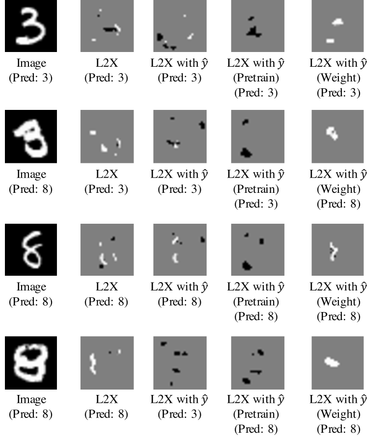
Figure 3. The example result of explanation on images from MNIST. The 4th row is the least confident sample of number “8”.

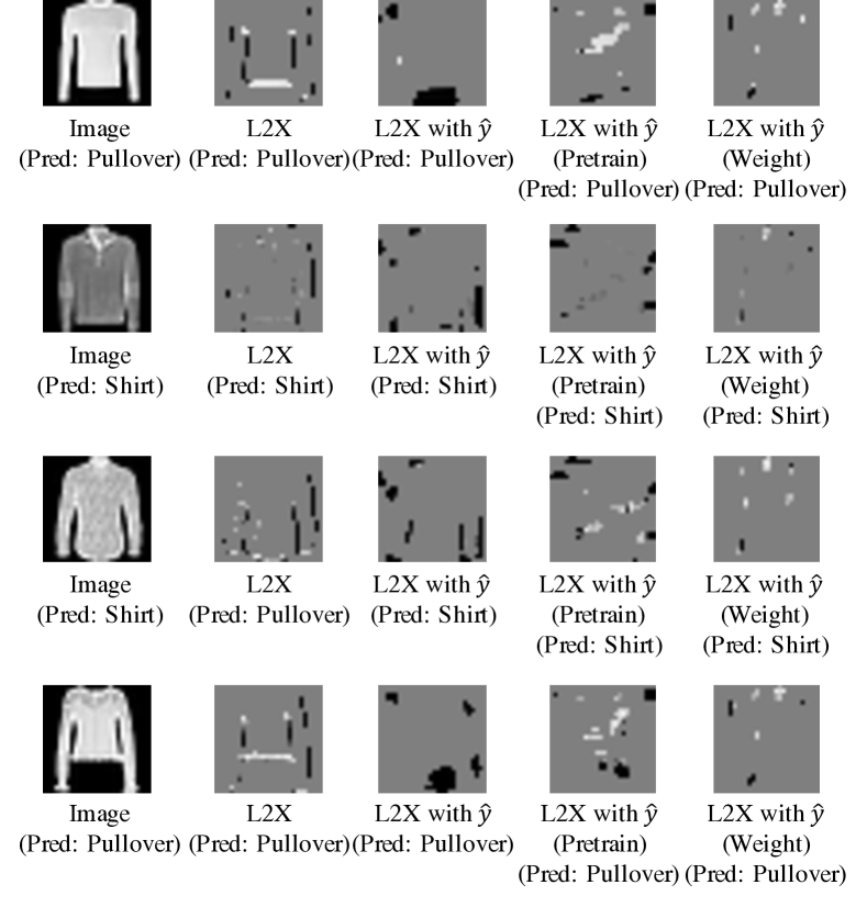
Figure 4. The example result of explanation on images from Fashion-MNIST.

F-MNIST  Figure 4 shows four examples from Fashion-MNIST. Similarly, the gray parts of images are unselected pixels, and the white/black parts are selected pixels.

Interestingly, we find that L2X tends to select the pixels on the edges. Similar to the examples of L2X in Table 4, the highlighted parts given by L2X may tend to be important generally, however, it may not be the most significant part for explaining the predictions of given models. On the other side, the explanations given by Weight tend to be of the neckline parts and the shoulder parts of the clothing, and maybe more informative to explain the predictions of machine learning models. For example, in the 3rd row of Figure 4, L2X selects the edges of the given image, while the model to be explained judges that the select features suggest that the image belongs to a Pullover.

6. Conclusion

Attention-based model interpretations have been popular for their convenience to integrate with neural networks. However, many researchers find that attention sometimes yields non-interpretable results, and there has been a debate on the interpretability of the attention mechanisms. This paper proposes that the combinatorial shortcuts are one of the root causes hindering attention mechanisms’ interpretability. We analyze the combinatorial shortcuts theoretically and design experiments to show their existence. Furthermore, we propose two methods to mitigate combinatorial shortcuts for better interpretability. Experiments show that the proposed methods effectively mitigate the adverse impacts and improve the interpretability of attention mechanisms. The results presented in this paper can help us better understand how attention mechanisms work.

Appendix A Details about the Evaluation Scheme

Here we present the structure of the models used for our experiments, as well as how the evaluation metrics are calculated.

A.1. The text classification models for IMDB and Yelp P.

Table 6. The structure of text classification models for IMDB and Yelp P.

Layer	# Units	Kernel Size	Stride	Padding	Activation
Embedding	50	– –	– –	– –	– –
Dropout ($0.2$)	– –	– –	– –	– –	– –
Convolution (1D)	250	3	1	default	ReLU
GlobalMaxPooling	– –	– –	– –	– –	– –
Fully-Connected	250	– –	– –	– –	ReLU
Dropout ($0.2$)	– –	– –	– –	– –	– –
Fully-Connected	2	– –	– –	– –	Softmax

The structure of neural network models to be explained for text classification datasets (including IMDB and Yelp P.) is presented in Table 6. This model structure achieved accuracy scores of about 96.1% and 89.0% on the train set and the test set of IMDB respectively, and about 96.0% and 95.4% on the train set and test set of Yelp P. respectively. The structures of explainers, as well as the approximators of models including L2X, VIBI, AIL, and L2X with $\hat{y}$ are slightly different from this to incorporate global information when selecting features and to select keywords. During our experiments, we find that while Pretrain prefers powerful approximators, Weight works more stable with simple approximators. This result is consistent with the results in Table 2. Besides, as estimating $\mathbb{E}(Y|X\odot M)$ requires good calibrations, layers that act differently during training and testing, like Dropout and BatchNormalization layers, may not be welcomed by explanation models.

A.2. The image classification model for MNIST and Fasion-MNIST

Table 7. The structure of image classification models for MNIST and Fashion-MNIST

Layer	# Units	Kernel Size	Stride	Padding	Activation
Convolution (2D)	32	(3, 3)	1	default	ReLU
Convolution (2D)	64	(3, 3)	1	default	ReLU
MaxPooling (2D)	– –	(2, 2)	(2, 2)	– –	– –
Flatten	– –	– –	– –	– –	– –
Dropout ($0.25$)	– –	– –	– –	– –	– –
Fully-Connected	128	– –	– –	– –	ReLU
Dropout ($0.5$)	– –	– –	– –	– –	– –
Fully-Connected	2	– –	– –	– –	Softmax

The structure of neural network models to be explained for image classification datasets (including MNIST and F-MNIST) is presented in Table 7. This model structure achieved accuracy scores of more than 99.8% on both the train set and test set of MNIST, and about 96.1% and 92.2% on the train set and test set of F-MNIST respectively. The structures of explainers, as well as the approximators of models including L2X, VIBI, AIL, and L2X with $\hat{y}$, are slightly different from this to incorporate global information and to select pixels.

A.3. Calculation of the evaluation metrics

The same with Chen et al. (2018) and Liang et al. (2020), we used post-hoc accuracy for quantitatively validating the effectiveness of the methods. After feature selection, unselected words of texts were filled with <PAD> tokens, and unselected pixels of images were filled with their average values. Then we used the model to be explained to predict the labels and compared whether the labels change or not. If the model makes consistent predictions before and after feature selection, the selected features may be informative for the model to make the decisions.

A.4. Brief introduction to the baseline methods

Among the baseline methods, Gradient (Simonyan et al., 2013) takes advantage of the property of neural networks and selects the input features which have the most significant absolute values of gradients. LIME (Ribeiro et al., 2016) explains a model by quantifying the model’s sensitivity to changes in the input. CXPlain (Schwab and Karlen, 2019) involves the real labels $y$ to compute the loss-function values by erasing each feature to zero and normalizes the loss-function values as the surrogate for ideal explanations for a neural network model to learn. Our methods follow the same paradigm as L2X (Chen et al., 2018), VIBI (Bang et al., 2019), and AIL (Liang et al., 2020), which use hard attention to select a fixed number of features to approximate the output of the original models to be explained. VIBI improves L2X to encourage the briefness of the learned explanation by adding a constraint for the feature scores to a global prior. AIL (Liang et al., 2020) is the state-of-the-art method that use adversarial training to encourage the gap between the predictability of selected/unselected features, additionally, AIL incorporate the outcome it aims to justify explicitly, as well as the gradients of the original model w.r.t. the samples to provide a warm start.

A.5. Comparison with adversarial solutions for improving interpretability

Liang et al. (2020) and Yu et al. (2019) also mentioned the phenomenon that attention could find a degenerated solution where attention could highlight feature components at different positions for different classes, and then the downstream parts of models may predict the label through this pattern, resulting in the lack of interpretability. And they used adversarial training to indirectly mitigate this combinatorial shortcut problem. However, they did not analyze why combinatorial shortcuts exist, and the adversarial scheme may change the behavioral tendency of models. For example, considering a sample with features $\{a,a^{\prime},b,b^{\prime},\text{noisy features}\}$, where $a^{\prime}$ is collinear with $a$, $b^{\prime}$ is collinear with $b$, and $a$ is relatively more predictive than $b$ while they are somehow complementary, the adversarial methods that encourage the gap between the predictability of selected/unselected features may tend to select $a$ and $a^{\prime}$ to maximum the gap, and fail to select $a$ and $b$ which might be more interpretable.

References

- (1)
- Bahdanau et al. (2015) Dzmitry Bahdanau, Kyunghyun Cho, and Yoshua Bengio. 2015. Neural Machine Translation by Jointly Learning to Align and Translate. In Proceedings of the International Conference on Learning Representations.
- Bai et al. (2020) Bing Bai, Guanhua Zhang, Ye Lin, Hao Li, Kun Bai, and Bo Luo. 2020. CSRN: Collaborative Sequential Recommendation Networks for News Retrieval. arXiv preprint arXiv:2004.04816 (2020).
- Bang et al. (2019) Seojin Bang, Pengtao Xie, Wei Wu, and Eric Xing. 2019. Explaining a Black-box using Deep Variational Information Bottleneck Approach. arXiv preprint arXiv:1902.06918 (2019).
- Belinkov and Glass (2019) Yonatan Belinkov and James Glass. 2019. Analysis methods in neural language processing: A survey. Transactions of the Association for Computational Linguistics 7 (2019), 49–72.
- Chakraborti et al. (2019) Tathagata Chakraborti, Anagha Kulkarni, Sarath Sreedharan, David E Smith, and Subbarao Kambhampati. 2019. Explicability? Legibility? Predictability? Transparency? Privacy? Security? The Emerging Landscape of Interpretable Agent Behavior. In Proceedings of the International Conference on Automated Planning and Scheduling, Vol. 29(1). 86–96.
- Chen et al. (2018) Jianbo Chen, Le Song, Martin Wainwright, and Michael Jordan. 2018. Learning to Explain: An Information-Theoretic Perspective on Model Interpretation. In International Conference on Machine Learning. 883–892.
- Choi et al. (2016) Edward Choi, Mohammad Taha Bahadori, Jimeng Sun, Joshua Kulas, Andy Schuetz, and Walter Stewart. 2016. RETAIN: An Interpretable Predictive Model for Healthcare Using Reverse Time Attention Mechanism. In Advances in Neural Information Processing Systems. 3504–3512.
- Clark et al. (2019) Kevin Clark, Urvashi Khandelwal, Omer Levy, and Christopher D Manning. 2019. What Does BERT Look at? An Analysis of BERT’s Attention. In Proceedings of the 2019 ACL Workshop BlackboxNLP: Analyzing and Interpreting Neural Networks for NLP. 276–286.
- Ertefaie and Stephens (2010) Ashkan Ertefaie and David A Stephens. 2010. Comparing Approaches to Causal Inference for Longitudinal Data: Inverse Probability Weighting Versus Propensity Scores. The International Journal of Biostatistics 6, 2 (2010).
- Fan et al. (2005) Wei Fan, Ian Davidson, Bianca Zadrozny, and Philip S Yu. 2005. An Improved Categorization of Classifier’s Sensitivity on Sample Selection Bias. In Proceedings of the Fifth IEEE International Conference on Data Mining. 605–608.
- Fu et al. (2016) Kun Fu, Junqi Jin, Runpeng Cui, Fei Sha, and Changshui Zhang. 2016. Aligning Where to See and What to Tell: Image Captioning with Region-based Attention and Scene-specific Contexts. IEEE Transactions on Pattern Analysis and Machine Intelligence 39, 12 (2016), 2321–2334.
- Jain and Wallace (2019) Sarthak Jain and Byron C Wallace. 2019. Attention is Not Explanation. In Proceedings of the 2019 Conference of the North American Chapter of the Association for Computational Linguistics: Human Language Technologies, Volume 1 (Long and Short Papers). 3543–3556.
- Jang et al. (2017) Eric Jang, Shixiang Gu, and Ben Poole. 2017. Categorical Reparametrization with Gumble-Softmax. In International Conference on Learning Representations.
- Lai et al. (2015) Siwei Lai, Liheng Xu, Kang Liu, and Jun Zhao. 2015. Recurrent Convolutional Neural Networks for Text Classification. In Proceedings of the Twenty-Ninth AAAI Conference on Artificial Intelligence. 2267–2273.
- LeCun et al. (1998) Yann LeCun, Léon Bottou, Yoshua Bengio, and Patrick Haffner. 1998. Gradient-based Learning Applied to Document Recognition. Proc. IEEE 86, 11 (1998), 2278–2324.
- Li et al. (2019) Yanwei Li, Xinze Chen, Zheng Zhu, Lingxi Xie, Guan Huang, Dalong Du, and Xingang Wang. 2019. Attention-guided Unified Network for Panoptic Segmentation. In Proceedings of the IEEE Conference on Computer Vision and Pattern Recognition. 7026–7035.
- Liang et al. (2020) Jian Liang, Bing Bai, Yuren Cao, Kun Bai, and Fei Wang. 2020. Adversarial Infidelity Learning for Model Interpretation. In Proceedings of the 26th ACM SIGKDD International Conference on Knowledge Discovery & Data Mining. 286–296.
- Lipton (2018) Zachary C Lipton. 2018. The Mythos of Model Interpretability. Queue 16, 3 (2018), 31–57.
- Maas et al. (2011) Andrew L Maas, Raymond E Daly, Peter T Pham, Dan Huang, Andrew Y Ng, and Christopher Potts. 2011. Learning Word Vectors for Sentiment Analysis. In Proceedings of the 49th Annual Meeting of the Association for Computational Linguistics: Human Language Technologies-volume 1. Association for Computational Linguistics, 142–150.
- Martins and Astudillo (2016) Andre Martins and Ramon Astudillo. 2016. From Softmax to Sparsemax: A Sparse Model of Attention and Multi-label Classification. In International Conference on Machine Learning. 1614–1623.
- Pennington et al. (2014) Jeffrey Pennington, Richard Socher, and Christopher D Manning. 2014. Glove: Global Vectors for Word Representation. In Proceedings of the 2014 Conference on Empirical Methods in Natural Language Processing (EMNLP). 1532–1543.
- Ribeiro et al. (2016) Marco Tulio Ribeiro, Sameer Singh, and Carlos Guestrin. 2016. “Why Should I Trust You?”: Explaining the Predictions of Any Classifier. In Proceedings of the 22nd ACM SIGKDD International Conference on Knowledge Discovery and Data Mining. ACM, 1135–1144.
- Rosenbaum and Rubin (1983) Paul R Rosenbaum and Donald B Rubin. 1983. The Central Role of the Propensity Score in Observational Studies for Causal Effects. Biometrika 70, 1 (1983), 41–55.
- Rubin (1974) Donald B Rubin. 1974. Estimating Causal Effects of Treatments in Randomized and Nonrandomized Studies. Journal of Educational Psychology 66, 5 (1974), 688.
- Schwab and Karlen (2019) Patrick Schwab and Walter Karlen. 2019. CXPlain: Causal Explanations for Model Interpretation Under Uncertainty. In Advances in Neural Information Processing Systems. 10220–10230.
- Serrano and Smith (2019) Sofia Serrano and Noah A Smith. 2019. Is Attention Interpretable?. In Proceedings of the 57th Annual Meeting of the Association for Computational Linguistics. 2931–2951.
- Shadish et al. (2008) William R Shadish, Margaret H Clark, and Peter M Steiner. 2008. Can Nonrandomized Experiments Yield Accurate Answers? A Randomized Experiment Comparing Random and Nonrandom Assignments. Journal of the American statistical association 103, 484 (2008), 1334–1344.
- Simonyan et al. (2013) Karen Simonyan, Andrea Vedaldi, and Andrew Zisserman. 2013. Deep Inside Convolutional Networks: Visualising Image Classification Models and Saliency Maps. arXiv preprint arXiv:1312.6034 (2013).
- Vapnik (1992) Vladimir Vapnik. 1992. Principles of Risk Minimization for Learning Theory. In Advances in Neural Information Processing Systems. 831–838.
- Vaswani et al. (2017) Ashish Vaswani, Noam Shazeer, Niki Parmar, Jakob Uszkoreit, Llion Jones, Aidan N Gomez, Łukasz Kaiser, and Illia Polosukhin. 2017. Attention is All You Need. In Advances in Neural Information Processing Systems. 5998–6008.
- Vinyals et al. (2015) Oriol Vinyals, Łukasz Kaiser, Terry Koo, Slav Petrov, Ilya Sutskever, and Geoffrey Hinton. 2015. Grammar as a Foreign Language. In Advances in Neural Information Processing Systems. 2773–2781.
- Wang et al. (2019) Fei Wang, Rainu Kaushal, and Dhruv Khullar. 2019. Should Health Care Demand Interpretable Artificial Intelligence or Accept “Black Box” Medicine? Annals of Internal Medicine (2019).
- Wang et al. (2016) Yequan Wang, Minlie Huang, Xiaoyan Zhu, and Li Zhao. 2016. Attention-based LSTM for Aspect-level Sentiment Classification. In Proceedings of the 2016 Conference on Empirical Methods in Natural Language Processing. 606–615.
- Wiegreffe and Pinter (2019) Sarah Wiegreffe and Yuval Pinter. 2019. Attention is not not Explanation. In Proceedings of the 2019 Conference on Empirical Methods in Natural Language Processing and the 9th International Joint Conference on Natural Language Processing (EMNLP-IJCNLP). 11–20.
- Winship and Morgan (1999) Christopher Winship and Stephen L Morgan. 1999. The Estimation of Causal Effects From Observational Data. Annual review of sociology 25, 1 (1999), 659–706.
- Xiao et al. (2017) Han Xiao, Kashif Rasul, and Roland Vollgraf. 2017. Fashion-MNIST: a Novel Image Dataset for Benchmarking Machine Learning Algorithms. arXiv preprint arXiv:1708.07747 (2017).
- Xu et al. (2015) Kelvin Xu, Jimmy Ba, Ryan Kiros, Kyunghyun Cho, Aaron Courville, Ruslan Salakhudinov, Rich Zemel, and Yoshua Bengio. 2015. Show, Attend and Tell: Neural Image Caption Generation with Visual Attention. In International Conference on Machine Learning. 2048–2057.
- Yu et al. (2019) Mo Yu, Shiyu Chang, Yang Zhang, and Tommi Jaakkola. 2019. Rethinking Cooperative Rationalization: Introspective Extraction and Complement Control. In Proceedings of the 2019 Conference on Empirical Methods in Natural Language Processing and the 9th International Joint Conference on Natural Language Processing (EMNLP-IJCNLP). 4085–4094.
- Zadrozny (2004) Bianca Zadrozny. 2004. Learning and Evaluating Classifiers Under Sample Selection Bias. In Proceedings of the Twenty-first International Conference on Machine Learning. 114.
- Zhang et al. (2019) Guanhua Zhang, Bing Bai, Jian Liang, Kun Bai, Shiyu Chang, Mo Yu, Conghui Zhu, and Tiejun Zhao. 2019. Selection Bias Explorations and Debias Methods for Natural Language Sentence Matching Datasets. In Proceedings of the 57th Annual Meeting of the Association for Computational Linguistics. 4418–4429.
- Zhang et al. (2020b) Guanhua Zhang, Bing Bai, Junqi Zhang, Kun Bai, Conghui Zhu, and Tiejun Zhao. 2020b. Demographics Should Not Be the Reason of Toxicity: Mitigating Discrimination in Text Classifications with Instance Weighting. In Proceedings of the 58th Annual Meeting of the Association for Computational Linguistics. 4134–4145.
- Zhang et al. (2020a) Junqi Zhang, Bing Bai, Ye Lin, Jian Liang, Kun Bai, and Fei Wang. 2020a. General-Purpose User Embeddings based on Mobile App Usage. In Proceedings of the 26th ACM SIGKDD International Conference on Knowledge Discovery & Data Mining. 2831–2840.
- Zhang et al. (2015) Xiang Zhang, Junbo Zhao, and Yann LeCun. 2015. Character-level Convolutional Networks for Text Classification. In Advances in Neural Information Processing Systems. 649–657.
- Zhu et al. (2017) Feng Zhu, Hongsheng Li, Wanli Ouyang, Nenghai Yu, and Xiaogang Wang. 2017. Learning Spatial Regularization with Image-level Supervisions for Multi-label Image Classification. In Proceedings of the IEEE Conference on Computer Vision and Pattern Recognition. 5513–5522.