Variational Optimization for the Submodular Maximum Coverage Problem

Abstract.

We examine the submodular maximum coverage problem (SMCP), which is related to a wide range of applications. We provide the first variational approximation for this problem based on the Nemhauser divergence, and show that it can be solved efficiently using variational optimization. The algorithm alternates between two steps: (1) an E step that estimates a variational parameter to maximize a parameterized modular lower bound; and (2) an M step that updates the solution by solving the local approximate problem. We provide theoretical analysis on the performance of the proposed approach and its curvature-dependent approximate factor, and empirically evaluate it on a number of public data sets and several application tasks.

1. Introduction

Submodular optimization lies at the core of many data mining and machine learning problems, ranging from summarizing massive data sets (badanidiyuru2014streaming, ; karbasi2018data, ), cutting and segmenting images (boykov2001interactive, ; kohli2008p3, ; jegelka2011submodularity, ), monitoring network status (leskovec2007cost, ; krause2008near, ), diversifying recommendation systems (mirzasoleiman2016fast, ; ashkan2015optimal, ), searching neural network architectures (xiong2019resource, ), interpreting machine learning models (elenberg2017streaming, ; lakkaraju2016interpretable, ; kim2016examples, ; ribeiro2016should, ), to asset management and risk allocation in finance (Acerbi12, ; ohsaka2017portfolio, ). Recent works have studied the optimization of submodular functions in various forms, for example, weighted coverage functions (feige1998threshold, ), rank functions of matroids (krause2009simultaneous, ), facility location functions (krause2008efficient, ), entropies (sharma2015greedy, ), as well as mutual information (krause2012near, ). In a typical setting, the optimization is subject to the classical cardinality constraint, where the number of elements selected is required to be under a preset constant limit. It’s been shown that even with this simple constraint, many submodular optimization problems are NP-hard, although under certain conditions the greedy algorithm can provide a good approximate solution (nemhauser1978analysis, ; vondrak2008optimal, ; wolsey1982analysis, ).

The forms of constraints in real applications are often very complex and may be given either analytically or in terms of value oracle models. We, therefore, investigate a more generalized formulation, i.e., the problems of maximizing a submodular function $g(X)$ subject to a general submodular upper bound constraint $f(X)\leq b$. This problem is referred to as the submodular maximum coverage problem (SMCP), or submodular maximization with submodular knapsack constraint (iyer2013submodular, ). The pioneer work (iyer2013submodular, ) first examined this problem and introduced an algorithms with bi-criterion approximation guarantees. The importance of SMCP has been widely recognized as it can be regarded as a meta-problem for a breadth of tasks including training the most accurate classifier subject to process unfairness constraints (grgic2018beyond, ), automatically design convolutional neural networks to maximize accuracy with a given forward time constraint (hu2019automatically, ), and selecting leaders in a social network for shifting opinions (yi2019shifting, ), to name a few.

While (iyer2013submodular, ) shows the greedy method with a modular approximation has good performance, we take a step further to build a mathematical connection between the variational modular approximation to a submodular function based on Namhauser divergence and classical variational approximation based on Kullback–Leibler divergence. We take advantage of this framework to iteratively solve SMCP, leading to a novel variational approach. Analogous to the counterpart of variational optimization based on Kullback-Leibler divergence, the proposed method consists of two alternating steps, namely estimation (E step) and maximization (M step) to monotonically improve the performance in an iterative fashion. We provide theoretical analysis on the performance of the proposed variational approach and prove that the E step provides the optimal estimator for the subsequent M step. More importantly, we show that the approximate factor of the EM algorithm is decided by the curvature of the objective function and the marginal gain of the constraint function. We evaluated the proposed framework on a number of public data sets and demonstrated it in several application tasks.

2. Problem Definition

2.1. Formulation

Submodularity is an important property that naturally exists in many real-world scenarios, for example, diminishing returns in economics (smith1937wealth, ), which refers to the phenomenon that the marginal benefit of any given element tend to decrease as more elements are added. Formally, let $[n]=\{1,2,\ldots,n\}$ be a finite ground set and the set of all subsets of $[n]$ be $2^{[n]}$. The real-valued discrete set function $f:2^{[n]}\to\mathbb{R}$ is submodular on $[n]$ if

(1) $$f(X)+f(Y)\geq f(X\cup Y)+f(X\cap Y)$$

holds for all $X,Y\subseteq[n]$ (fujishige2005submodular, ). We denote a singleton set with element $j$ as $\{j\}$ and the marginal gain as $f(j|X)\triangleq f(j\cup X)-f(X)$. The marginal gain is also known as the discrete derivative of $f$ at $X$ with respect to $j$, and we use $\Delta_{f}$ to denote the maximum marginal gain at $X=\emptyset$:

(2) $$\Delta_{f}=\max_{j\in[n]}f(j).$$

In terms of the marginal gain, the submodularity defined in (1) is equivalent to

(3) $$f(j|X)\geq f(j|Y),\ \forall X\subseteq Y\subseteq[n],\ j\notin Y.$$

Intuitively, the monotonicity means $f$ won’t decrease as $X$ is expanded. A necessary and sufficient monotone condition for $f$ is that all its discrete derivatives are nonnegative, i.e., $f(j|X)\geq 0$, for all $j\notin X$ and $X\subseteq[n]$.

Our primary interest is the aa (SMCP):

(4) $$\max_{X}~{}g(X),\quad\mathrm{s.t.}~{}~{}f(X)\leq b,$$

where $f(X)$ and $g(X)$ are monotone, and are assumed to be normalized such that $f(\emptyset)=0$ and $g(\emptyset)=0$. Our formulation is general enough with minimal assumptions, the techniques developed in this paper, including the analysis, are applicable to general forms of $g(X)$ and $f(X)$, including those with analytical forms or given in terms of a value oracle.

Fig 1 illustrates a concrete example of SMCP, where we are given a bipartite graph consisting of two kinds of nodes, i.e., square nodes and circle nodes; each circle node is associated with a non-negative value, and each square node represents a singleton; the goal is to select a subset, $X$, out of the square nodes, such that the circle nodes being covered have as much total value (denoted by $g(X)$) as possible yet the number of circle node selected is within a set limit, i.e., $f(X)<b$.

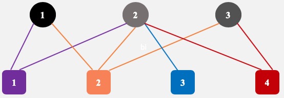
Figure 1. A bipartite graph to illustrate an SMCP problem. Each square node covers at least one circle node. Different square nodes is allowed to cover the same circle node, and each circle node associates a nonnegative value. The goal is to find a subset of the square nodes covering maximum total value, yet with the number of circle nodes smaller than $b$.

2.2. Related Problems

The SMCP problem was first studied in (iyer2013submodular, ), where it was also referred to as submodular cost with submodular knapsack constraint (SCKC). The authors further established the equivalence between SMCP (4) and minimizing $f(X)$ subject to $g(X)\geq c$ (called submodular cost with submodular cover constraint or SCSC). A greedy algorithm and an ellipsoidal approximation method were employed to solve SMCP in (iyer2013submodular, ).

SMCP is regarded as a meta-problem to many application tasks, of which we introduce a few examples. In (grgic2018beyond, ), it was shown that training a classifier with fairness constraints involves solving a variant of SMCP, where $X$ is the feature subset, and both the objective (i.e., loss function) and constraints are submodular. (hu2019automatically, ) studied automatically designing convolutional neural networks (CNNs) to maximize accuracy within a given forward time constraint, where $X$ represents the configuration of a CNN (e.g, kernel size at each layer) and $f(X)$ is the forward time function. It’s shown that the validation accuracy on a held out set of samples is submdoular (xiong2019resource, ). (kempe2003maximizing, ) investigated influence maximization in social networks and show the influence function is submodular, although the formulation is unconstrained. (yi2019shifting, ) studied French-Degroot opinion dynamics in a social network with two polarizing parties to shift opinions in a social network through leader selection. In their formulation, $g(X)$ is the influence function and $f(X)$ is the average opinion of all nodes, both of which are submodular. In finance, the conditional value at risk (CVaR) is well known and widely used for risk control and portfolio management, for example, (ohsaka2017portfolio, ) examined the maximization of CVaR to select portfolios based on a formulation similar to SMCP, and employed a greedy method to solve it.

Cardinality-constrained submodular maximization is a special case of SMCP since the candinality $|X|$ is a modular function. A number of important tasks can be approached by this simpler variant of SMCP, for example, data set summarization (badanidiyuru2014streaming, ; karbasi2018data, ), network status monitoring (leskovec2007cost, ; krause2008near, ), and interpretable machine learning (elenberg2017streaming, ; kim2016examples, ; ribeiro2016should, ).

3. Variational Bounds

A submodular function resembles both convex functions and concave functions (iyer2013submodular, ), in the sense that it can be bounded both from above and below. In this section, we propose variational SMCP (V-SMCP), a variational approximate for SMCP based on Nemhauser divergence.

3.1. Upper Bound for $f(X)$

In the seminal work (nemhauser1978analysis, ), it is demonstrated that the submodularity of $f(X)$ in (1) is equivalent to the following inequality

(5) $$\underbrace{f(X)-\sum_{j\in X\backslash Y}f(j|X\backslash j)+\sum_{j\in Y\backslash X}f(j|\Theta)}_{\triangleq\widehat{f}_{X}(Y;\Theta)}\geq f(Y),\ \forall X,Y\subseteq[n],$$

where $\Theta=X\cap Y$. Following from the above inequality, the Nemhauser divergence (iyer2012submodular, ) between two set functions $\widehat{f}_{X}(Y;\Theta)$ and $f(Y)$ is defined as

(6) $$\mathcal{D}(\widehat{f}_{X}(Y;\Theta)||f(Y))=\widehat{f}_{X}(Y;\Theta)-f(Y),$$

which satisfies $\mathcal{D}(\widehat{f}_{X}(Y;\Theta)||f(Y))\geq 0$. The equality holds when $X=Y$, which implies $\Theta=Y$. The Nemhauser divergence measures the distance between two set functions and is not symmetric, which is similar to the Kullback-Leibler divergence that measures the distance between two probability distributions.

Note that (nemhauser1978analysis, ) provids another inequality, which is also equivalent to the submodularity of $f(X)$, given by

(7) $$\underbrace{f(X)+\sum_{j\in Y\backslash X}f(j|X)-\sum_{j\in X\backslash Y}f(j|\Psi\backslash j)}_{\triangleq\widehat{f}_{X}(Y;\Psi)}\geq f(Y),\ \forall X,Y\subseteq[n],$$

with $\Psi=X\cup Y$. We can therefore define the divergence with $\widehat{f}_{X}(Y;\Psi)$, i.e., $\mathcal{D}(\widehat{f}_{X}(Y;\Psi)||f(Y))=\widehat{f}_{X}(Y;\Psi)-f(Y)$ for the variational optimization. Yet, as there is no guarantee that which one between these two functions provides a better approximation, we focus on $\mathcal{D}(\widehat{f}_{X}(Y;\Theta)||f(Y))$ in this paper, and all the algorithms and analyses provided can be adapted to the algorithm based on $\mathcal{D}(\widehat{f}_{X}(Y;\Psi)||f(Y))$.

3.2. Lower Bound for $g(X)$

We define a permutation on the elements of $[n]$, i.e., $\pi:[n]\to[n]$ that orders the elements in $[n]$ as a sequence $\left(\pi_{1},\pi_{2},\ldots,\pi_{n}\right)$, which denotes that if $\pi_{i}=j$, $j$ is the $i$-th element in this sequence. Particularly, given a subset $X_{t}\subseteq 2^{[n]}$, we choose a permutation $\pi$ that places the elements in $X_{t}$ first and then includes the remaining elements in $[n]\backslash X_{t}$, where the subscript $t$ denotes the iteration number used in the EM algorithm introduced in the next section. We further define the corresponding sequence of subsets of $[n]$ as $S^{\pi}_{i}$ with $i=0,\ldots,n$, which is given by

(8) $$S^{\pi}_{0}=\emptyset,\ S^{\pi}_{1}=\{\pi_{1}\},\ \ldots,\ S^{\pi}_{n}=\{\pi_{1},\ldots,\pi_{n}\},$$

which results in $\emptyset=S^{\pi}_{0}\subset S^{\pi}_{1}\subset S^{\pi}_{2}\ldots\subset S^{\pi}_{n}=[n]$. Then a lower bound of $g(X)$ is given by (iyer2013submodular, )

(9) $$\widehat{g}^{\pi}_{X_{t}}(X)=\sum_{j\in X}\widehat{g}^{\pi}_{X_{t}}(j),\ \forall X\subset[n],$$

where $\widehat{g}^{\pi}_{X_{t}}(j)$ with $j=\pi_{i}$ is defined by (iyer2013submodular, )

(10) $$\widehat{g}^{\pi}_{X_{t}}(j)=\widehat{g}^{\pi}_{X_{t}}(S_{i}^{\pi}-S^{\pi}_{i-1})=g(S_{i}^{\pi})-g(S^{\pi}_{i-1}).$$

Since $X_{t}$ and $\pi$ has a mapping relationship, in the following of the paper, we omit the superscript $\pi$ when no confusing is caused. The lower bound property, i.e., $\widehat{g}_{X_{t}}(X)\leq g(X)$ can be easily proved (iyer2013submodular, ) according to the submodularity. Further more, substituting (10) into (9) and considering the permutation given by $\pi$, it guarantees the tightness at $X_{t}$ that

(11) $$\widehat{g}_{X_{t}}(X_{t})=g(X_{t}).$$

3.3. Variational Approximation for SMCP

The SMCP in (4) can be approximated, at any given $X_{t}$, by the following problem, which we call V-SMCP:

(12) $$\max_{X}{}{}{}{} \widehat{g}_{X_{t}}(X)$$

$$\quad\mathrm{s.t.}{}{}{}{} \widehat{f}_{X_{t}}(X;\widehat{\Theta}_{t})\leq b,$$

$$\widehat{\Theta}_{t}=\mathop{\mathrm{argmin}}_{\Theta}\mathcal{D}(\widehat{f}_{X_{t}}(X;\Theta)||f(X)),$$

$$\Theta=X\cap X_{t},$$

where $\widehat{g}_{X_{t}}(X)$ and $\widehat{f}_{X_{t}}(X;\widehat{\Theta}_{t})$ are lower bound and upper bound for $g(X)$ and $f(X)$, respectively. V-SMCP is an effective approximation of SMCP as both bounds are tight at $X_{t}$, i.e., $\widehat{g}_{X_{t}}(X_{t})=g(X_{t})$ and $\widehat{f}_{X_{t}}(X_{t};X_{t})=f(X_{t})$.

4. Variational Optimization

In this section, we introduce an iterative method to solve an SMCP based on a sequence of V-SMCPs. It alternates between (1) an estimation (E) step that minimizes the Namhauser divergence by estimating the parametric approximation; and (2) a subsequent maximization (M) step that updates the solution.

Since $\widehat{f}_{X_{t}}(X;\Theta)$ is an upper bound of $f(X)$, maximizing $\widehat{f}_{X_{t}}(X;\Theta)$ w.r.t $\Theta$ will equivalently minimizing $\mathcal{D}_{\Theta}(\widehat{f}_{X_{t}}(X;\Theta)||f(X))$. We therefore treat $\Theta$ as a variational parameter and estimate it in the E step to reduce $\mathcal{D}_{\Theta}(\widehat{f}_{X_{t}}(X;\Theta)||f(X))$ as much as possible. Then with $\Theta=\widehat{\Theta}_{t}$, we update the solution by solving a V-SMCP in the M step. We name this method estimation-maximization (EM) algorithm.

4.1. E step: Estimate $\widehat{\Theta}_{t}$

According to the submodularity definition in (3), we have $f(j|\Theta_{1})\geq f(j|\Theta_{2})$ if $\Theta_{1}\subseteq\Theta_{2}$. Following from (7), for all $X\subseteq[n]$, we further obtain

(13) $$\widehat{f}_{X_{t}}(X;\Theta_{1})\geq\widehat{f}_{X_{t}}(X;\Theta_{2}),\ \forall\Theta_{1}\subseteq\Theta_{2}.$$

This inequality indicates that we can decrease the divergence of $\mathcal{D}(\widehat{f}_{X_{t}}(X;\Theta)||f(X))$ by enlarging $\Theta$. Thus, the largest $\Theta$ is $X_{t}$, according to the Nemhauser divergence defined in (7). To avoid notational clumsiness, we use $E\backslash j$ to denote a set that excludes $j$, i.e.,

(14) $$E{\backslash j}=\left\{\begin{aligned} &X_{t}\backslash j,&\textrm{if}\ j\in X_{t},\\ &X_{t},&\textrm{if}\ j\notin X_{t}.\end{aligned}\right.$$

By substituting (14) to (7), we define a permutation operation $\epsilon:[n]\to[n]$ that orders the elements in $[n]$ as a sequence $\left(\epsilon_{1},\epsilon_{2},\ldots,\epsilon_{n}\right)$ such that

(15) $$\frac{\widehat{g}_{X_{t}}(\epsilon_{1})}{f(\epsilon_{1}|E\backslash{\epsilon_{1}})}\geq\frac{\widehat{g}_{X_{t}}(\epsilon_{2})}{f(\epsilon_{2}|E\backslash{\epsilon_{2}})}\geq\ldots\geq\frac{\widehat{g}_{X_{t}}(\epsilon_{n})}{f(\epsilon_{n}|E\backslash{\epsilon_{n}})}.$$

There must exist a $\widehat{k}$ such that

$$\widehat{k}=\mathop{\mathrm{argmax}}_{k}\sum_{k^{\prime}=1}^{k}f(\epsilon_{k^{\prime}}|E_{\epsilon_{k}})\leq b.$$

We then obtain an estimation of $\Theta$ given by

(16) $$\widehat{\Theta}_{t}=X_{t}\cap\widehat{X}_{t},$$

with

(17) $$\widehat{X}_{t}=\{\epsilon_{1},\epsilon_{2},\ldots,\epsilon_{\widehat{k}}\}.$$

While there is no guarantee that $\widehat{f}_{X_{t}}(\widehat{X}_{t};\widehat{\Theta}_{t})\leq b$ is satisfied, the estimator $\widehat{\Theta}_{t}$ as well as $\widehat{X}_{t}$ would lead to a larger feasible space for maximizing $\widehat{g}_{X_{t}}(X)$ in the subsequent M step, which is analytically proved in Section 5.

4.2. M Step: Compute the Maximizer $X_{t+1}$

For notational brief, in the M step, we represent a set without $j$ given $X_{t}$ as

(18) $$M\backslash j=\left\{\begin{aligned} &X_{t}\backslash j,\ \textrm{if}\quad j\in X_{t},\\ &\widehat{\Theta}_{t},\quad\textrm{if}\quad j\notin X_{t}.\end{aligned}\right.$$

Substituting (18) to (7), we further define a new permutation $\mu:[n]\to[n]$ that orders the elements in $[n]$ as a new sequence $\left(\mu_{1},\mu_{2},\ldots,\mu_{n}\right)$ such that

(19) $$\frac{\widehat{g}_{X_{t}}(\mu_{1})}{f(\mu_{1}|M\backslash{\mu_{1}})}\geq\frac{\widehat{g}_{X_{t}}(\mu_{2})}{f(\mu_{2}|M\backslash{\mu_{2}})}\ldots\geq\frac{g_{X_{t}}(\mu_{n})}{f(\mu_{n}|M\backslash{\mu_{n}})}.$$

By letting $\widehat{m}$ be the largest index that satisfy the following inequality:

(20) $$\widehat{m}=\mathop{\mathrm{argmax}}_{m}\sum_{m^{\prime}=1}^{m}f(\mu_{m^{\prime}}|M_{\mu_{m^{\prime}}})\leq b,$$

we finally obtain the optimizer at the $t$-th iteration:

(21) $$X_{t+1}=\{\mu_{1},\mu_{2},\ldots,\mu_{\widehat{m}}\}.$$

From (9), the corresponding objective value is

(22) $$\widehat{g}(X_{t+1})=\sum_{m^{\prime}=1}^{\widehat{m}}g_{X_{t}}(\mu_{m^{\prime}}).$$

The algorithm terminates once $\widehat{g}(X_{t+1})\leq\widehat{g}(X_{t})$, which is equivalent to $g(X_{t+1})\leq g(X_{t})$ according to (11). The proposed EM algorithm is summarized in Algorithm 1. Note that in both E step and M step, the permutation $\epsilon$ and $\mu$ can be implemented in $\mathcal{O}(n\log{}n)$ time through any efficient sorting procedure.

Fig.  2 shows how the EM algorithm approximates the solution of P1 in the space of $2^{[n]}\times\mathbb{R}$. The black curve represents the objective function under constraint in SMCP. At the $t$-th iteration, we construct $\widehat{g}_{X_{t}}(X)$ with tightness guarantee at $X_{t}$ according to (11). In the E step, we compute $\widehat{\Theta}_{t}$ to enlarge the feasible space, in the subsequent M step, we compute $X_{t+1}$, which is the approximate solution for P2. The corresponding function is shown by the red curve. Then at the $(t+1)$-th, we compute the new lower bound with estimation $\widehat{\Theta}_{t+1}$ depicted by the blue color.

A simplified version of EM algorithm can be obtained by setting $\widehat{\Theta}_{t}=\emptyset$ in the EM algorithm. This simplified EM (SEM) method saves the computation cost for the permutation $\epsilon$ in the E step. We summarize the SEM in Algorithm 2. However, it is evident that the E step of EM algorithm leads to larger or equal (when $\widehat{\Theta}=\emptyset$ in (16)) feasible space than the SEM algorithm. Therefore, it is guaranteed that the EM algorithm has a no smaller objective value than SEM, which is also verified by experiments in Section 6.

0:  Initialization: $X_{0}$ {EM Algorithm.}

1:  while $\widehat{g}_{X_{t}}(X_{t})\leq g_{X_{t}}(X_{t+1})$ do

2:     E Step:

3:     Compute $\widehat{X}_{t}$ via (17).

4:     Update $\widehat{\Theta}_{t}$ via (16).

5:     M Step:

6:     Update $X_{t+1}$ via (21).

7:  end while

Algorithm 1 EM algorithm.

0:  Initialization: $X_{0}$ {SEM Algorithm.}

1:  while $\widehat{g}_{X_{t}}(X_{t})\leq g_{X_{t}}(X_{t+1})$ do

2:     E Step:

3:     Set $\widehat{\Theta}_{t}=\emptyset$.

4:     M Step:

5:     Update $X_{t+1}$ via (21).

6:  end while

Algorithm 2 SEM algorithm

5. Theoretical Analysis

In this section, we provide analysis of the proposed EM algorithm. By replacing $X$ and $Y$ in (7) with $X_{t}$ and $X_{t+1}$, we obtain

(23) $$b\geq\underbrace{f(X_{t})-\sum_{j\in X_{t}\backslash X_{t+1}}f(j|X_{t}\backslash j)+\sum_{j\in X_{t+1}\backslash X_{t}}f(j|\Theta)}_{=\widehat{f}_{X_{t}}(X_{t+1};\Theta)}\geq f(X_{t+1}).$$

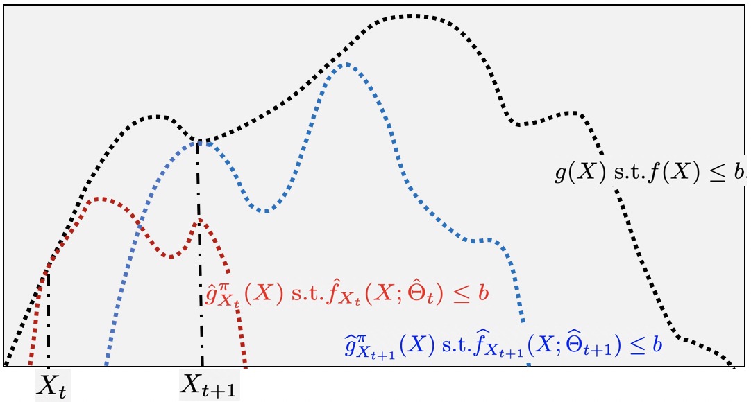
Figure 2. The alternating process of the proposed EM algorithm, which involves computing a lower bound with maximum feasible space and then maximizing this lower bound to update the optimizer.

The quantities $\Theta=X_{t}\cap X$ implies that $\emptyset\subseteq\Theta\subseteq X_{t}$. According to (13), we have $\widehat{f}_{X_{t}}(X;\emptyset)\geq\widehat{f}_{X_{t}}(X;\Theta)\geq\widehat{f}_{X_{t}}(X;X_{t})$. Thus, $\widehat{f}_{X_{t}}(X;X_{t})$ is the tightest bound we can achieve. In spite of this, we cannot simply set $\widehat{\Theta}_{t}=X_{t}$ since it is unsecured that $X_{t+1}$, which is obtained in the M step, satisfies $X_{t}\cap X_{t+1}=X_{t}$. Then there is no warranty that $\widehat{f}_{X_{t}}(X_{t+1};X_{t})\geq f(X_{t+1})$. Consequently, $f(X_{t+1})<b$ is not guaranteed, and $X_{t+1}$ may not lies in the feasible space, which violates the constraint in (12). In the following theorem, we analytically show the optimality of $\widehat{\Theta}_{t}$ (equation (16) in the proposed E step). Here, an optimal $\widehat{\Theta}_{t}$ implies that it provides the feasible space which is a superset of all the feasible space provided by any other $\Theta_{t}$’s.

Theorem 5.1 (Optimality).

In the E step of the EM algorithm, $\widehat{\Theta}_{t}$, i.e., equation (16), provides the optimal $\Theta_{t}$ for the optimization problem in the M step at each iteration.

Proof.

Because in the E step, we have no idea about the $X_{t+1}$, we need to estimate a $\widehat{\Theta}_{t}$ such that for all possible $X_{t+1}$, the constraint $f(X_{t+1})\leq\widehat{f}_{X_{t}}(X;\Theta)$ is always satisfied, so that $f(X_{t+1})\leq b$ is guaranteed. Thus, according to $(\ref{Nemhauster_divergence1})$, we need to show that $f(j|\widehat{\Theta}_{t})$ is larger than any $f(j|\Theta_{t})$. We prove this as follows.

First, according to (16), we have $\emptyset\subseteq\widehat{\Theta}_{t}\subseteq X_{t}$. Then, (13) shows that setting $\widehat{\Theta}_{t}=X_{t}$ leads to the smallest $f(\epsilon_{i}|E\backslash\epsilon_{i})$. At last, due to the sorting mechanism in (15), the solution $\widehat{X}_{t}$ is the smallest subset containing elements from all possible $X_{t+1}$, which makes any $\Theta_{t}$ that satisfies $\emptyset\subseteq\Theta_{t}\subseteq\widehat{X}_{t}\cap X_{t}$ is a subset of $X_{t+1}\cap X_{t}$. Thus, we conclude that $\forall X_{t+1}$, $f(X_{t+1})\leq\widehat{f}_{X_{t}}(X_{t+1};\Theta_{t})$ if $\emptyset\leq\Theta_{t}\leq\widehat{X}_{t}\cap X_{t}$. Hence, in the feasible range, the optimal $\Theta$ is obtained by setting $\widehat{\Theta}_{t}=\widehat{X}_{t}\cap X_{t}$ as it gives the smallest $\widehat{f}_{X_{t}}(X_{t+1};\Theta_{t})$, i.e.,

$$\widehat{f}_{X_{t}}(X_{t+1};\widehat{\Theta}_{t})\leq\widehat{f}_{X_{t}}(X_{t+1};\Theta_{t})$$

for all the feasible $\Theta_{t}$. Therefore, it leads to the largest feasible space. ∎

Proposition 5.2 (Monotonicity).

The EM algorithm monotonically improves the objective function value, i.e., $g(X)$ in the feasible space of SMCP, i.e., $g(X_{0})\leq g(X_{1})\leq g(X_{2})\leq\ldots$.

Proof.

According to the tightness property in (11), we have $g(X_{t})=\widehat{g}_{X_{t}}(X_{t})$. Since the proposed EM algorithm leads to increment of $\widehat{g}_{X_{t}}(X)$ at each iteration, we obtain $\widehat{g}_{X_{t}}(X_{t})\leq\widehat{g}_{X_{t}}(X_{t+1})$. Moreover, the lower bound property of $\widehat{g}_{X_{t}}(X)$ results in $\widehat{g}_{X_{t}}(X_{t+1})\leq g(X_{t+1})$. Therefore, we obtain $g(X_{t})\leq g(X_{t+1})$. Hence, the monotonicity of the EM algorithm is proved. ∎

We next provide tightened, curvature-dependent approximation ratio for the proposed algorithms. Curvature has served to improve the approximation ratio for submodular maximization problems, e.g., from $(1-\frac{1}{e})$ to $\frac{1}{\kappa_{g}}(1-e^{-\kappa_{g}})$ for monotone submodular maximization subject to a cardinality constraint (conforti1984submodular, ) and matroid constraints (vondrak2010submodularity, ). We first give the definition of curvature and then analytically prove our results.

Given a submodular function $g$, the curvature $\kappa_{g}$, which represents the deviation from modularity, is defined as

(24) $$\kappa_{g}=1-\min_{k\in[n]}\frac{g(k|[n]\setminus k)}{g(k)}.$$

The curvature, $\kappa_{g}$ measures the distance of $g$ from modularity, and $\kappa_{g}=0$ if and only if $g$ is modular, i.e., $g(X)=\sum_{j\in X}g(j)$. Next, we show the approximation ratio of $\widehat{g}(X)$ to $g(X)$ in terms of curvature.

Theorem 5.3 (Function $\widehat{g}$ Approximation Ratio).

Given arbitrary $\pi$ and $X_{t}$, the approximation ratio given by $\widehat{g}_{X_{t}}(X)$ to $g(X)$ is $1-\kappa_{g}$, i.e.,

(25) $$\widehat{g}_{X_{t}}(X)\geq(1-\kappa_{g})g(X),\quad\forall X\subseteq[n].$$

Proof.

The definition of $\widehat{g}(j)$ in (10) is equivalently represented by $\widehat{g}_{X_{t}}(j)=g(S_{j}^{\pi})-g(S^{\pi}_{j-1})=g(j|S^{\pi}_{j-1})$ for all $j\in[n]$. Then, according to (3), we have $\widehat{g}_{X_{t}}(j)=g(j|S^{\pi}_{j-1})\geq g(j|[n]\backslash j)$. Dividing both sides by a positive number $g(j)$, we have

(26) $$\frac{\widehat{g}_{X_{t}}(j)}{g(j)}\geq\frac{g(j|[n]\backslash j)}{g(j)}\geq\min_{k\in[n]}\frac{g(k|[n]\backslash k)}{g(k)},\quad\forall j\in[n].$$

The most right-hand side of the above inequality is $1-\kappa_{g}$ according to the curvature definition in (24). We therefore obtain

(27) $$\frac{\widehat{g}_{X_{t}}(j)}{g(j)}\geq 1-\kappa_{g},\quad\forall j\in[n].$$

Next, we extend the above inequality from an arbitrary element $j\in[n]$ to an arbitrary set $X\subseteq[n]$ by induction. Equation (27) implies that

(28) $$\frac{\widehat{g}_{X_{t}}(j_{1})+\widehat{g}_{X_{t}}(j_{2})}{g(j_{1})+g(j_{2})}\geq 1-\kappa_{g},\quad\forall j_{1},j_{2}\in[n].$$

Then by induction, we have

(29) $$\frac{\sum_{j\in X}\widehat{g}_{X_{t}}(j)}{\sum_{j\in X}g(j)}\geq 1-\kappa_{g},\quad\forall X\subseteq[n].$$

The numerator in the left-hand side of the above inequality is equivalent to $\widehat{g}_{X_{t}}(X)$ from (9). Furthermore, the submodularity of $g(X)$ indicates $g(X)\leq\sum_{j\in X}g(j)$. Therefore, we can further magnify the left-hand side of (29) and obtain

(30) $$\frac{\widehat{g}_{X_{t}}(X)}{g(X)}\geq\frac{\sum_{j\in X}\widehat{g}_{X_{t}}(j)}{\sum_{j\in X}g(j)}\geq 1-\kappa_{g},\quad\forall X\subseteq[n].$$

∎

Next, we show the approximation ratio of the proposed EM/SEM algorithm for $\widehat{g}_{X_{t}}(X)$ in a V-SMCP. Let $\textrm{OPT}_{\widehat{g}_{X_{t}}}$ denote the optimizer for (12).

Proposition 5.4.

At each iteration, both the EM and SEM algorithms obtain a set $X_{t+1}$ such that

(31) $$\widehat{g}_{X_{t}}(X_{t+1})\geq(1-\frac{2\Delta_{f}}{b})\widehat{g}_{X_{t}}(\textrm{OPT}_{\widehat{g}_{X_{t}}}).$$

The tedious but straightforward proof for this proposition is provided in the Appendix. Yet, this proposition paves the way to the proof of the approximation ratio of the EM algorithm for $g(X)$ in V-SMCP. Let OPT denote the optimizer for (4), and with the knowledge of Theorem 5.3 and Proposition 5.4 in mind, w be have the following result.

Theorem 5.5 (Approximate Optimality).

The results of both EM and SEM algorithm, i.e., $g(X_{t+1})$ hold the approximation ratio $(1-\kappa_{g})(1-\frac{2\Delta_{f}}{b})$, i.e.,

(32) $$g(X_{t+1})\geq(1-\kappa_{g})(1-\frac{2\Delta_{f}}{b})g(\textrm{OPT}).$$

Proof.

Since $\textrm{OPT}_{\widehat{g}_{X_{t}}}$ is the optimizer of $\widehat{g}_{X_{t}}(X)$, we have the inequality $\widehat{g}(\textrm{OPT}_{\widehat{g}_{X_{t}}})\geq\widehat{g}(\textrm{OPT})\geq 0$. Further, due to $g(X)\geq 0$ for all $X\subseteq[n]$, and following from (25), we obtain $\widehat{g}(\textrm{OPT})\geq 0$. We then have $\widehat{g}_{X_{t}}(\textrm{OPT}_{\widehat{g}_{X_{t}}})\geq\widehat{g}_{X_{t}}(\textrm{OPT})\geq 0,$ which results in

(33) $$\frac{g(\textrm{OPT})}{\widehat{g}_{X_{t}}(\textrm{OPT}_{\widehat{g}_{X_{t}}})}\leq\frac{g(\textrm{OPT})}{\widehat{g}_{X_{t}}(\textrm{OPT})}\leq\frac{1}{1-\kappa_{g}},$$

where the second inequality is due to Theorem 5.3 by replacing $X$ with OPT in (25). Then, we obtain

$$\widehat{g}_{X_{t}}(\textrm{OPT}_{\widehat{g}_{X_{t}}})\geq(1-\kappa_{g})g(\textrm{OPT}).$$

Substituting (31) to the left-hand side of the above inequality, we obtain

$$\widehat{g}_{X_{t}}(X_{t+1})\geq(1-\kappa_{g})(1-\frac{2\Delta_{f}}{b})g(\textrm{OPT}).$$

∎

6. Experiments

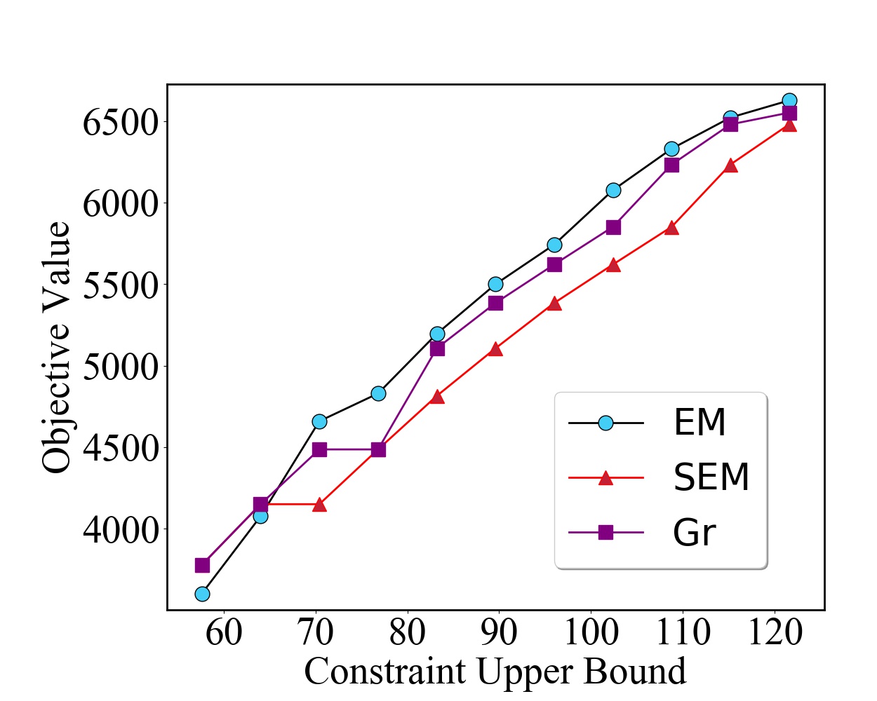
(a) PCodes Dataset

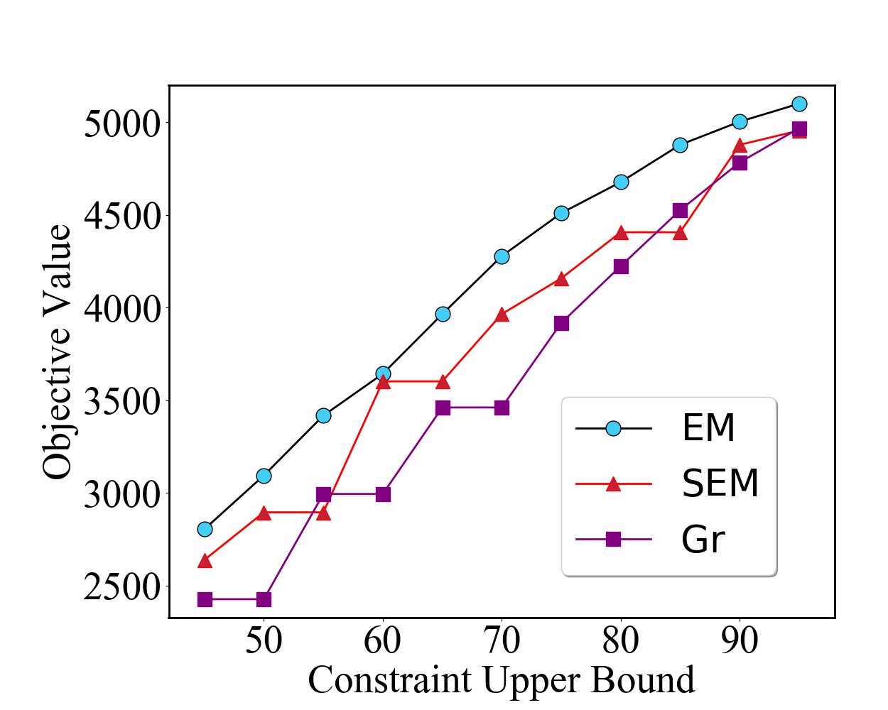
(b) Gap-A

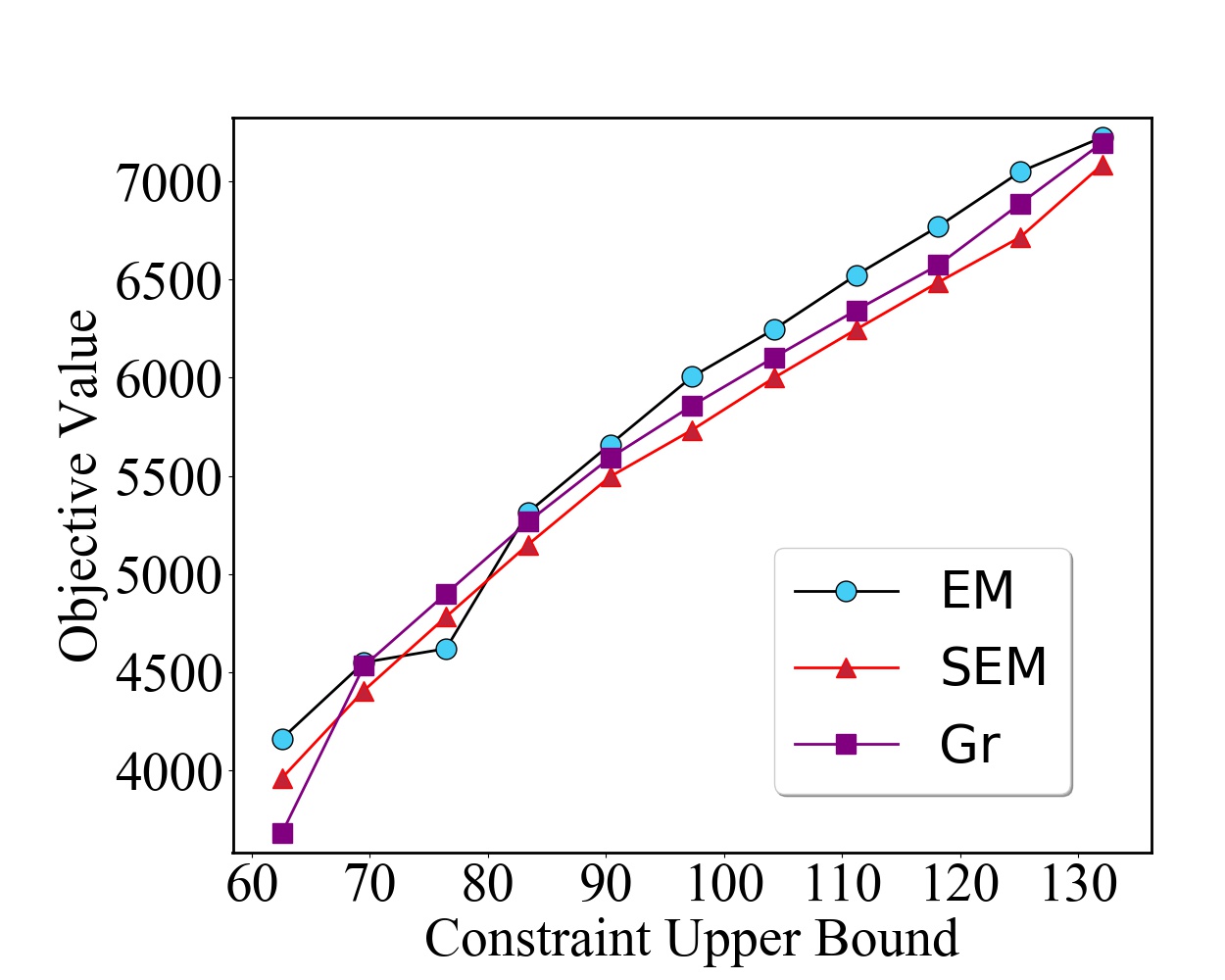
(c) Chess

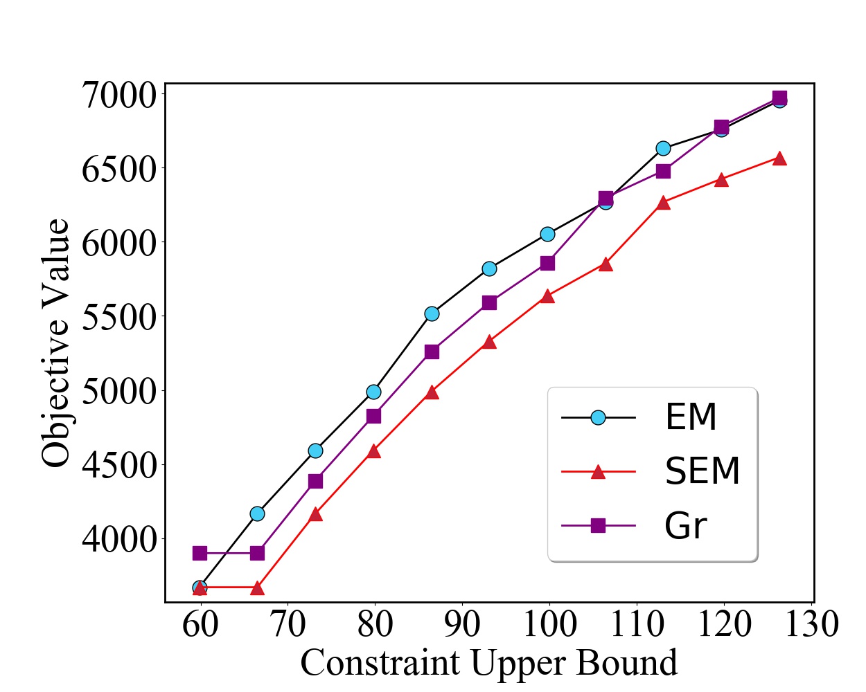
(d) FPP

Figure 3. Comparison of objective values with public data sets.

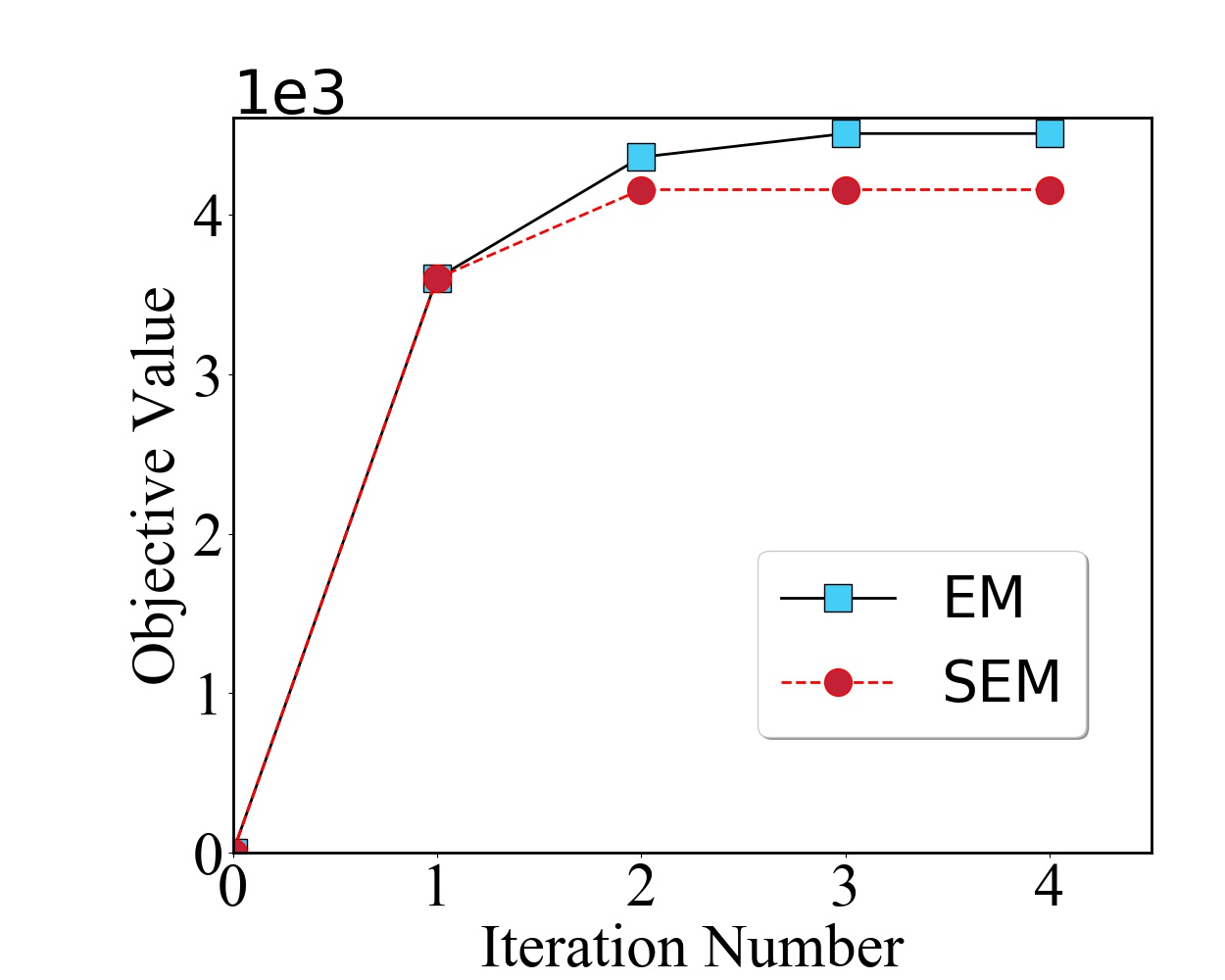
(a) Upper bound: 65.

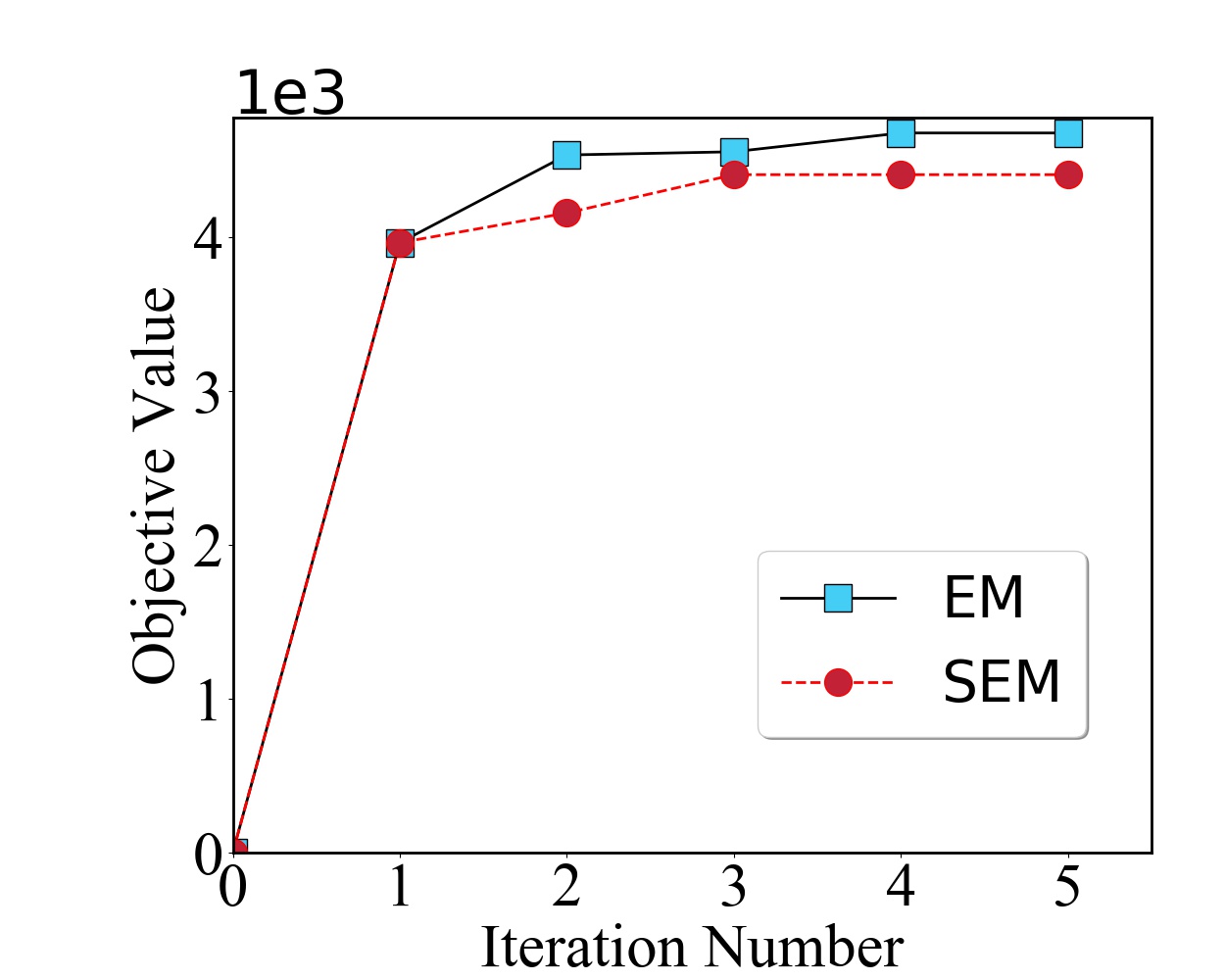
(b) Upper bound: 70.

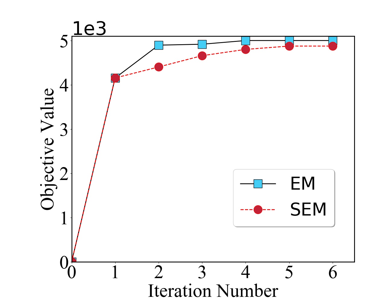
(c) Upper bound: 85.

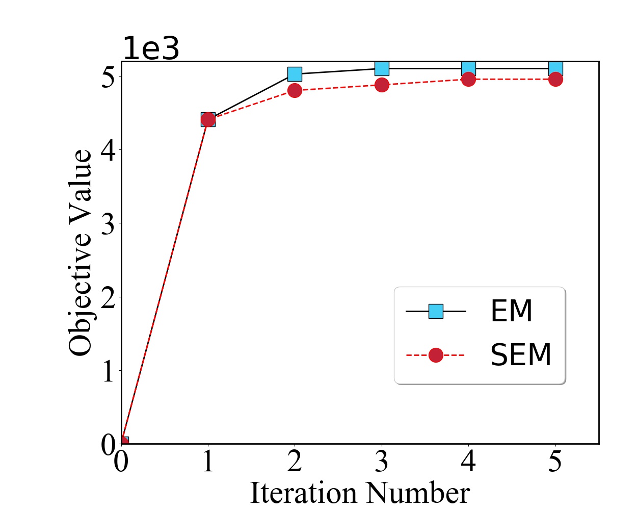
(d) Upper bound: 90.

Figure 4. Convergence and monotonicity of EM and SEM algorithms with different upper-bound constraints for the Gap-A data set.

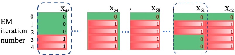
Figure 5. ${X_{i}}$ updating process of the EM algorithm. In this example, the $61$-th element was first selected in the $1$-st iteration and later removed in the $3$-rd iteration.

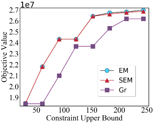
(a) Data Set 1

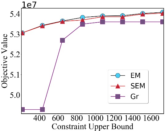
(b) Data Set 2

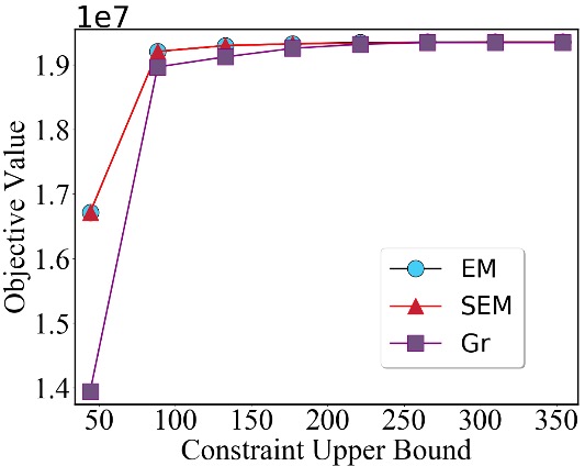
(c) Data Set 3

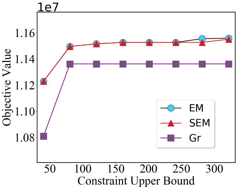
(d) Data Set 4

Figure 6. Comparison of objective values with different settings for the $4$ different data sets.

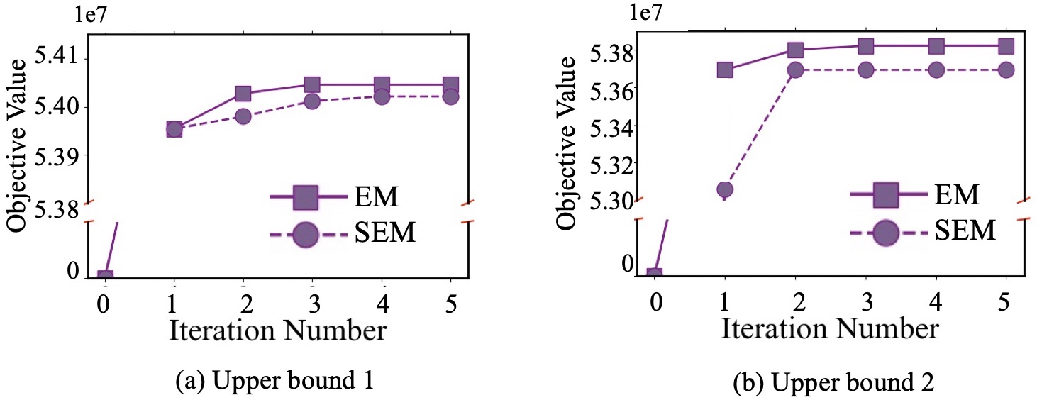
Figure 7. Convergence and monotonicity of EM and SEM algorithms with two different upper-bound constraints.

Since first proposed in (iyer2013submodular, ), the SMCP has been identified for a breadth of applications ranging from training the most accurate classifier subject to process unfairness constraints (grgic2018beyond, ), automatically designing convolutional neural networks to maximize accuracy within a given forward time constraint (hu2019automatically, ) to shifting opinions in a social network through leader selection (yi2019shifting, ).

In order to understand the mechanism, effectiveness, and application potential of the proposed variational framework and EM algorithm for SMCP, we start on the public data set and demonstrate the performance advantages over existing methods. After that, we test the performance in the production environment, first on decision rule selection for fraud transaction detection, and then go further to train a interpretable classifier that covers truth positive in the feature space well, and control the false positive within a predefined bound due to production requirement.

6.1. Performance on Discrete Location Data Sets

To compare the performance of our EM algorithm with that of existing methods, we consider four bipartite graphs from the public discrete location data sets (FLdata, ) including an instance on perfer codes (PCodes), an instance on chess-board (Chess), an instance on finite projective planes (FPP), and an instance on large duality gap (Gap-A) with $128$, $144$, $133$, and $100$ nodes for each type of the corresponding bipartite graphs, respectively. For more detailed information of these data sets, please refer to (FLdata, ). Fig. 1 is a running example of this test. A random value, which is uniformly sampled from $1$ to $100$, is assigned to each circle node, and our goal is to choose a subset of the square nodes to maximize the total sum-value of the covered circle nodes subject to an upper bound constraint of the total number of the square nodes.

We compare the greedy (Gr) algorithm, which was proposed in the classical work (iyer2013submodular, ) and has been widely applied for different applications. Without an E step, it is analogous to the M step in the EM algorithm with a permutation $\epsilon$ such that

(34) $$\widetilde{\epsilon}(i)\in\operatorname{argmax}\left\{g\left(j|S_{i-1}^{\pi}\right)|j\notin S_{i-1}^{\pi},f\left(S_{i-1}^{\pi}\cup\{j\}\right)\leq b\right\}.$$

It was shown that Gr shows best performance in most experiments in (iyer2013submodular, ). We, therefore, compare the EM algorithm with the Gr as well as the SEM algorithms. The ellipsoidal approximation method in (iyer2013submodular, ) is not applied here due to high computational complexity.

By considering $11$ upper bounds in each kind of data set, we thus compare the performances of different algorithms in a total of $44$ experiments. As shown in Fig. 3, our EM algorithm outperforms all other methods in all the $44$ experiments except the only case when the upper bound is $60$ in the FPP data set. Gr algorithms and SEM have overlaps with each other in some settings, yet most of the time Gr outperforms SEM. Interestingly, in the sub-figure (b), we notice that the Gr algorithm’s objective values cannot be increased when the constraint upper bound is increased from $55$ to $60$ as well as from $65$ to $70$. SEM also suffers from the same problem when the constraint upper bound is increased from $50$ to $55$, $60$ to $65$, and $80$ to $85$. Similar problems can also be identified for Gr and SEM in other data sets. However, it is rare to happen to EM. Thus, the experiment demonstrates that our EM algorithm, which enlarges the approximate feasible space in the E step, makes a better use of the feasible space of the SMCP.

We further test the convergence rate and the monotonicity of the EM algorithm by fixing the data set to be Gap-A and choosing four different upper bounds, i.e., $65$, $70$, $85$, and $90$. Fig. 4 shows the objective value versus EM/SEM iteration number. It demonstrates that our EM algorithm converges quickly within $3$-$5$ iterations, and the objective value increases monotonically, which is consistent with Proposition 2. Note that as the initial values are set to be $\emptyset$, the first updates of EM and SEM are the same and hence the corresponding objective values after first iterations are the same.

To get deeper insight of the EM algorithm, we further demonstrate part of the updating process of it. We take the computing for PCodes data set as an example and set the bound to be $60$. As shown in Fig. 5, $X_{61}$ was first selected in the first and second iterations and later was removed in the third iteration. In contrast to the Gr algorithm, which keeps expanding the solution set by adding new element, our EM algorithm select solutions dynamically. This dynamic provides the capability to obtain a better result.

Table 1. Summary of transaction data set

# samples	# fraud	# normal	# features	# categorical features	# continuous features
50,357	369	49,988	50	26	24

Table 2. Classification performance

Method	Fraud coverage	Interruption rate
Decision Tree	82.16$\%$	1.05$\%$
EM	83.73$\%$	0.96$\%$

6.2. Performance on Fraud Detection Data Sets

Beyond the public data set experiment, we go further to a practical applications. In our online payment systems, we have a bunch of rules for detecting fraud transactions. Some of them are obtained based on humans experience, and some of them are given by machine learning models like decision tree. Some of these rules could be too aggressive that not only covers the frauds but also interrupt a lot of normal transactions. Our goal is to select rules that can cover as much fraud amounts as possible and in the meantime to make sure the interrupted transaction amount below a predefined value.

We consider four data sets in four different local areas, where each area has their own detection rules due to different attributes in each area. Each data set consists of transaction index and their labels (fraud or not), and the list of rules that cover each transaction. There are in total of $1200$, $10052$, $1600$, and $2400$ transactions in each data set, and the number of rules are $85$, $98$, $112$, and $92$ respectively.

As shown in Fig. 6 that our EM algorithm outperforms all other methods consistently for different upper bounds as well as in different data sets. Furthermore, Fig. 7 shows the objective value of as a function of the iteration number for data set 2 with different upper bounds. It is demonstrated that our EM algorithm also converges quickly within $3$-$5$ iterations in the industrial environment.

6.3. Application to Interpretable Classifier

Following the same context of fraud detection, we further go beyond the rules selection scenario by modeling the problem as designing an iterpretable classifier based on SMCP. From the lens of the classier, we are interested in maximizing the true positive subject to an upper bounded false negative.

More specifically, given a bunch of features for each transactions, we first apply the efficient F-P algorithm (han2000mining, ) for mining the frequent fraud transaction patterns/rules. We limit the maximum rule length to be $4i$ to make it more interpretable. Let $[n]$ denote the set of rules obtained. To detect as many fraud value as possible (which is equivalently to maximize the truth positive), we maximize the following objective function:

$$g(X)=v\left(\cup_{i\in X}\mathcal{C}\mathcal{R}(i)\right),$$

where $X\subseteq[n]$, $\mathcal{C}\mathcal{R}(r_{i})$ is the set of frauds covered by rule $i$, and $v(\cdot)$ is the total amount of fraud transaction value covered by $X$. Moreover, the number of interrupted transactions, i.e., normal transactions but classified mistakenly, can be denoted by

$$f(X)=\left|\cup_{i\in X}\mathcal{C}(i)\setminus\mathcal{CR}(i)\right|,$$

where $\mathcal{C}(i)$ denotes all the transactions covered by rule $i$, either correctly or wrongly. We then can train a classifier that is consist of the rules selected by maximizing $g(X)$ subjective to an constraint that $f(X)<b$. According to the submodularity definition in (3), both $f(X)$ and $g(X)$ are monotonic submodular functions. Consequently, training the classifer is equivalent to solving an SMCP. We therefore apply our EM algorithm to train this classifier.

We summarize the data set in Table 1 and split $75\%$ of the data into a training set and $25\%$ of the data into a testing set. For performance comparison, we choose a decision tree with a maximum depth of $4$. We summarize the result in Table 2. It shows that the EM based method achieves performance that covers more fraud amount and also achieves less interruptions. The advantages could come from the formulation that builds the classifier, which exchanges false positive and true negative to identify as many frauds as possible in the feasible space.

7. Conclusions

In this paper, we have proposed a novel variational frame based on the Namhauser divergence for the submodular maximum coverage problem (SMCP). The proposed estimation-and-maximization (EM) method monotonically improves optimization performance in a few iterations. We have further proved a curvature dependent approximate factor for the EM method. Empirical results on both public data sets and industrial problems in production environment have shown evident performance improvement over state-of-the-art algorithms.

Appendix A Proof of Proposition 5.4

For the independence of the appendix, we repeat (19) with the first $\widehat{m}+1$ terms as below.

(35) $$\frac{\widehat{g}^{\pi}_{X_{t}}(\mu_{1})}{f(\mu_{1}|M\backslash{\mu_{1}})}\geq\frac{\widehat{g}^{\pi}_{X_{t}}(\mu_{2})}{f(\mu_{2}|M\backslash{\mu_{2}})}\ldots\geq\frac{\widehat{g}^{\pi}_{X_{t}}(\mu_{\widehat{m}+1})}{f(\mu_{\widehat{m}+1}|M\backslash{\mu_{\widehat{m}+1}})}.$$

Then by induction we have

(36) $$\frac{\sum_{k=1}^{\widehat{m}+1}\widehat{g}^{\pi}_{X_{t}}(\mu_{k})}{\sum_{k=1}^{\widehat{m}+1}f(\mu_{k}|M\backslash{\mu_{k}})}\geq\frac{\widehat{g}^{\pi}_{X_{t}}(\mu_{\widehat{m}+1})}{f(\mu_{\widehat{m}+1}|M\backslash{\mu_{\widehat{m}+1}})}.$$

According to the definition of $\widehat{m}$ in (20), it is evident that

$$\sum_{k=1}^{\widehat{m}+1}f(\mu_{k}|M\backslash{\mu_{k}})\geq b.$$

Substituting the above inequality to (36), it holds that

(37) $$\begin{split}g^{\pi}_{X_{t}}(\mu_{\widehat{m}+1})&\leq\frac{1}{b}f(\mu_{\widehat{m}+1}|M\backslash{\mu_{\widehat{m}+1}})\sum_{k=1}^{\widehat{m}+1}g^{\pi}_{X_{t}}(\mu_{k})\\ &\leq\frac{1}{b}f(\mu_{\widehat{m}+1}|\emptyset)\sum_{k=1}^{\widehat{m}+1}g^{\pi}_{X_{t}}(\mu_{k})\\ &\leq\frac{\Delta_{f}}{b}\sum_{k=1}^{\widehat{m}+1}g^{\pi}_{X_{t}}(\mu_{k}).\end{split}$$

The second inequality is due to (13), and the third inequality follows from $f(\emptyset)=0$ as well as (2). By subtracting $\frac{\Delta_{f}}{b}g^{\pi}_{X_{t}}(\mu_{\widehat{m}+1})$ on the left-hand side and then adding $\sum_{k=1}^{\widehat{m}}g^{\pi}_{X_{t}}(\mu_{k})$ on both sides, we obtain

(38) $$\begin{split}\sum_{k=1}^{\widehat{m}}g^{\pi}_{X_{t}}(\mu_{k})+(1-\frac{\Delta_{f}}{b})g^{\pi}_{X_{t}}(\mu_{\widehat{m}+1})\leq\frac{\Delta_{f}}{b}\sum_{k=1}^{\widehat{m}+1}g^{\pi}_{X_{t}}(\mu_{k})+\sum_{k=1}^{\widehat{m}}g^{\pi}_{X_{t}}(\mu_{k}),\end{split}$$

which equals

(39) $$\begin{split}\sum_{k=1}^{\widehat{m}+1}g^{\pi}_{X_{t}}(\mu_{k})-\frac{\Delta_{f}}{b}g^{\pi}_{X_{t}}(\mu_{\widehat{m}+1})\leq\frac{\Delta_{f}}{b}\sum_{k=1}^{\widehat{m}+1}g^{\pi}_{X_{t}}(\mu_{k})+\sum_{k=1}^{\widehat{m}}g^{\pi}_{X_{t}}(\mu_{k}),\end{split}$$

The above inequality still holds after subtracting a positive $\sum_{k=1}^{\widehat{m}}g^{\pi}_{X_{t}}(\mu_{k})$ on the left-hand side:

(40) $$\begin{split}(1-\frac{2\Delta_{f}}{b})\sum_{k=1}^{\widehat{m}+1}g^{\pi}_{X_{t}}(\mu_{k})\leq\sum_{k=1}^{\widehat{m}}g^{\pi}_{X_{t}}(\mu_{k}).\end{split}$$

From (22) $\sum_{k=1}^{\widehat{m}}g^{\pi}_{X_{t}}(\mu_{k})=\widehat{g}(X_{t+1})$, and considering the fact that $\sum_{k=1}^{\widehat{m}+1}g^{\pi}_{X_{t}}(\mu_{k})\geq\textrm{OPT}_{\widehat{g}}$, we finally prove Proposition 5.4:

$$\widehat{g}(X_{t+1})\geq(1-\frac{2\Delta_{f}}{b})\widehat{g}({\textrm{OPT}_{\widehat{g}}}).$$

References

- (1) Ashwinkumar Badanidiyuru, Baharan Mirzasoleiman, Amin Karbasi, and Andreas Krause. Streaming submodular maximization: Massive data summarization on the fly. In Proceedings of the 20th ACM SIGKDD international conference on Knowledge discovery and data mining, pages 671–680, 2014.
- (2) Amin Karbasi, Ehsan Kazemi, Marko Mitrovic, and Morteza Zadimoghaddam. Data summarization at scale: A two-stage submodular approach. In ICML, 2018.
- (3) Yuri Y Boykov and M-P Jolly. Interactive graph cuts for optimal boundary & region segmentation of objects in nd images. In Proceedings eighth IEEE international conference on computer vision. ICCV 2001, volume 1, pages 105–112. IEEE, 2001.
- (4) Pushmeet Kohli, M Pawan Kumar, and Philip HS Torr. P3 & beyond: Move making algorithms for solving higher order functions. IEEE Transactions on Pattern Analysis and Machine Intelligence, 31(9):1645–1656, 2008.
- (5) Stefanie Jegelka and Jeff Bilmes. Submodularity beyond submodular energies: coupling edges in graph cuts. In CVPR 2011, pages 1897–1904. IEEE, 2011.
- (6) Jure Leskovec, Andreas Krause, Carlos Guestrin, Christos Faloutsos, Jeanne VanBriesen, and Natalie Glance. Cost-effective outbreak detection in networks. In Proceedings of the 13th ACM SIGKDD international conference on Knowledge discovery and data mining, pages 420–429, 2007.
- (7) Andreas Krause, Ajit Singh, and Carlos Guestrin. Near-optimal sensor placements in gaussian processes: Theory, efficient algorithms and empirical studies. Journal of Machine Learning Research, 9(Feb):235–284, 2008.
- (8) Baharan Mirzasoleiman, Morteza Zadimoghaddam, and Amin Karbasi. Fast distributed submodular cover: Public-private data summarization. In Advances in Neural Information Processing Systems, pages 3594–3602, 2016.
- (9) Azin Ashkan, Branislav Kveton, Shlomo Berkovsky, and Zheng Wen. Optimal greedy diversity for recommendation. In Twenty-Fourth International Joint Conference on Artificial Intelligence, 2015.
- (10) Yunyang Xiong, Ronak Mehta, and Vikas Singh. Resource constrained neural network architecture search: Will a submodularity assumption help? In Proceedings of the IEEE International Conference on Computer Vision, pages 1901–1910, 2019.
- (11) Ethan Elenberg, Alexandros G Dimakis, Moran Feldman, and Amin Karbasi. Streaming weak submodularity: Interpreting neural networks on the fly. In Advances in Neural Information Processing Systems, pages 4044–4054, 2017.
- (12) Himabindu Lakkaraju, Stephen H Bach, and Jure Leskovec. Interpretable decision sets: A joint framework for description and prediction. In Proceedings of the 22nd ACM SIGKDD international conference on knowledge discovery and data mining, pages 1675–1684, 2016.
- (13) Been Kim, Rajiv Khanna, and Oluwasanmi O Koyejo. Examples are not enough, learn to criticize! criticism for interpretability. In Advances in neural information processing systems, pages 2280–2288, 2016.
- (14) Marco Tulio Ribeiro, Sameer Singh, and Carlos Guestrin. ” why should i trust you?” explaining the predictions of any classifier. In Proceedings of the 22nd ACM SIGKDD international conference on knowledge discovery and data mining, pages 1135–1144, 2016.
- (15) Carlo Acerbi and Dirk Tasche. Expected shortfall: A natural coherent alternative to value at risk. Economic Notes, 31(2):379–388, 2002.
- (16) Naoto Ohsaka and Yuichi Yoshida. Portfolio optimization for influence spread. In Proceedings of the 26th International Conference on World Wide Web, pages 977–985, 2017.
- (17) Uriel Feige. A threshold of ln n for approximating set cover. Journal of the ACM (JACM), 45(4):634–652, 1998.
- (18) Andreas Krause, Ram Rajagopal, Anupam Gupta, and Carlos Guestrin. Simultaneous placement and scheduling of sensors. In 2009 International Conference on Information Processing in Sensor Networks, pages 181–192. IEEE, 2009.
- (19) Andreas Krause, Jure Leskovec, Carlos Guestrin, Jeanne VanBriesen, and Christos Faloutsos. Efficient sensor placement optimization for securing large water distribution networks. Journal of Water Resources Planning and Management, 134(6):516–526, 2008.
- (20) Dravyansh Sharma, Ashish Kapoor, and Amit Deshpande. On greedy maximization of entropy. In International Conference on Machine Learning, pages 1330–1338, 2015.
- (21) Andreas Krause and Carlos E Guestrin. Near-optimal nonmyopic value of information in graphical models. In UAI 2005: Proceedings of the Twenty-First Conference on Uncertainty in Artificial Intelligence, 2005.
- (22) George L Nemhauser, Laurence A Wolsey, and Marshall L Fisher. An analysis of approximations for maximizing submodular set functions—i. Mathematical programming, 14(1):265–294, 1978.
- (23) Jan Vondrák. Optimal approximation for the submodular welfare problem in the value oracle model. In Proceedings of the fortieth annual ACM symposium on Theory of computing, pages 67–74, 2008.
- (24) Laurence A Wolsey. An analysis of the greedy algorithm for the submodular set covering problem. Combinatorica, 2(4):385–393, 1982.
- (25) Rishabh K Iyer and Jeff A Bilmes. Submodular optimization with submodular cover and submodular knapsack constraints. In Advances in Neural Information Processing Systems, pages 2436–2444, 2013.
- (26) Nina Grgić-Hlača, Muhammad Bilal Zafar, Krishna P Gummadi, and Adrian Weller. Beyond distributive fairness in algorithmic decision making: Feature selection for procedurally fair learning. In Thirty-Second AAAI Conference on Artificial Intelligence, 2018.
- (27) Wenzheng Hu, Junqi Jin, Tie-Yan Liu, and Changshui Zhang. Automatically design convolutional neural networks by optimization with submodularity and supermodularity. IEEE Transactions on Neural Networks and Learning Systems, 2019.
- (28) Yuhao Yi, Timothy Castiglia, and Stacy Patterson. Shifting opinions in a social network through leader selection. arXiv preprint arXiv:1910.13009, 2019.
- (29) Adam Smith. The wealth of nations, 2018.
- (30) Satoru Fujishige. Submodular functions and optimization. Elsevier, 2005.
- (31) David Kempe, Jon Kleinberg, and Éva Tardos. Maximizing the spread of influence through a social network. In Proceedings of the ninth ACM SIGKDD international conference on Knowledge discovery and data mining, pages 137–146, 2003.
- (32) Rishabh Iyer and Jeff A Bilmes. Submodular-bregman and the lovász-bregman divergences with applications. In Advances in Neural Information Processing Systems, pages 2933–2941, 2012.
- (33) Michele Conforti and Gérard Cornuéjols. Submodular set functions, matroids and the greedy algorithm: tight worst-case bounds and some generalizations of the rado-edmonds theorem. Discrete applied mathematics, 7(3):251–274, 1984.
- (34) Jan Vondrák. Submodularity and curvature: The optimal algorithm (combinatorial optimization and discrete algorithms). 2010.
- (35) Vladimir Beresnev, Yuri Kochetov, Mihail Pashchenko, Alexander Kononov, Eugeni Goncharov, Alexander Plyasunov, Nina Kochetova, Ekaterina Alekseeva, and Ivanenko Dmitry. Discrete location problems–benchmark library. http://www.math.nsc.ru/AP/benchmarks/english.html. Accessed February 11, 2020.
- (36) Jiawei Han, Jian Pei, and Yiwen Yin. Mining frequent patterns without candidate generation. ACM sigmod record, 29(2):1–12, 2000.