Contrastive Multi-View Representation Learning on Graphs

Abstract

We introduce a self-supervised approach for learning node and graph level representations by contrasting structural views of graphs. We show that unlike visual representation learning, increasing the number of views to more than two or contrasting multi-scale encodings do not improve performance, and the best performance is achieved by contrasting encodings from first-order neighbors and a graph diffusion. We achieve new state-of-the-art results in self-supervised learning on 8 out of 8 node and graph classification benchmarks under the linear evaluation protocol. For example, on Cora (node) and Reddit-Binary (graph) classification benchmarks, we achieve 86.8% and 84.5% accuracy, which are 5.5% and 2.4% relative improvements over previous state-of-the-art. When compared to supervised baselines, our approach outperforms them in 4 out of 8 benchmarks.

1 Introduction

Graph neural networks (GNN) (Li et al., 2015; Gilmer et al., 2017; Kipf & Welling, 2017; Veličković et al., 2018; Xu et al., 2019b) reconcile the expressive power of graphs in modeling interactions with unparalleled capacity of deep models in learning representations. They process variable-size permutation-invariant graphs and learn low-dimensional representations through an iterative process of transferring, transforming, and aggregating the representations from topological neighbors. Each iteration expands the receptive field by one-hop and after $k$ iterations the nodes within $k$-hops influence one another (Khasahmadi et al., 2020). GNNs are applied to data with arbitrary topology such as point clouds (Hassani & Haley, 2019), meshes (Wang et al., 2018), robot designs (Wang et al., 2019), physical processes (Sanchez-Gonzalez et al., 2018), social networks (Kipf & Welling, 2017), molecules (Duvenaud et al., 2015), and knowledge graphs (Vivona & Hassani, 2019). For an overview see (Zhang et al., 2020; Wu et al., 2020).

GNNs mostly require task-dependent labels to learn rich representations. Nevertheless, annotating graphs is challenging compared to more common modalities such as video, image, text, and audio. This is partly because graphs are usually used to represent concepts in specialized domains, e.g., biology. Also, labeling graphs procedurally using domain knowledge is costly (Sun et al., 2020). To address this, unsupervised approaches such as reconstruction based methods (Kipf & Welling, 2016) and contrastive methods (Li et al., 2019) are coupled with GNNs to allow them learn representations without relying on supervisory data. The learned representations are then transferred to a priori unknown down-stream tasks. Recent works on contrastive learning by maximizing mutual information (MI) between node and graph representations have achieved state-of-the-art results on both node classification (Veličković et al., 2019) and graph classification (Sun et al., 2020) tasks. Nonetheless, these methods require specialized encoders to learn graph or node level representations.

Recent advances in multi-view visual representation learning (Tian et al., 2019; Bachman et al., 2019; Chen et al., 2020), in which composition of data augmentations is used to generate multiple views of a same image for contrastive learning, has achieved state-of-the-art results on image classification benchmarks surpassing supervised baselines. However, it is not clear how to apply these techniques to data represented as graphs. To address this, we introduce a self-supervised approach to train graph encoders by maximizing MI between representations encoded from different structural views of graphs. We show that our approach outperforms previous self-supervised models with significant margin on both node and graph classification tasks without requiring specialized architectures. We also show that when compared to supervised baselines, it performs on par with or better than strong baselines on some benchmarks.

To further improve contrastive representation learning on node and graph classification tasks, we systematically study the major components of our framework and surprisingly show that unlike visual contrastive learning: (1) increasing the number of views, i.e., augmentations, to more than two views does not improve the performance and the best performance is achieved by contrasting encodings from first-order neighbors and a general graph diffusion, (2) contrasting node and graph encodings across views achieves better results on both tasks compared to contrasting graph-graph or multi-scale encodings, (3) a simple graph readout layer achieves better performance on both tasks compared to hierarchical graph pooling methods such as differentiable pooling (DiffPool) (Ying et al., 2018), and (4) applying regularization (except early-stopping) or normalization layers has a negative effect on the performance.

Using these findings, we achieve new state-of-the-art in self-supervised learning on 8 out of 8 node and graph classification benchmarks under the linear evaluation protocol. For example, on Cora node classification benchmark, our approach achieves 86.8% accuracy, which is a 5.5% relative improvement over previous state-of-the-art (Veličković et al., 2019), and on Reddit-Binary graph classification benchmark, it achieves 84.5% accuracy, i.e., a 2.4% relative improvement over previous state-of-the-art (Sun et al., 2020). When compared to supervised baselines, our approach performs on par with or better than strong supervised baselines, e.g., graph isomorphism network (GIN) (Xu et al., 2019b) and graph attention network (GAT) (Veličković et al., 2018), on 4 out of 8 benchmarks. As an instance, on Cora (node) and IMDB-Binary (graph) classification benchmarks, we observe 4.5% and 5.3% relative improvements over GAT, respectively.

2 Related Work

2.1 Unsupervised Representation Learning on Graphs

Random walks (Perozzi et al., 2014; Tang et al., 2015; Grover & Leskovec, 2016; Hamilton et al., 2017) flatten graphs into sequences by taking random walks across nodes and use language models to learn node representations. They are shown to over-emphasize proximity information at the expense of structural information (Veličković et al., 2019; Ribeiro et al., 2017). Also, they are limited to transductive settings and cannot use node features (You et al., 2019).
Graph kernels (Borgwardt & Kriegel, 2005; Shervashidze et al., 2009, 2011; Yanardag & Vishwana, 2015; Kondor & Pan, 2016; Kriege et al., 2016) decompose graphs into sub-structures and use kernel functions to measure graph similarity between them. Nevertheless, they require non-trivial task of devising similarity measures between substructures.
Graph autoencoders (GAE) (Kipf & Welling, 2016; Garcia Duran & Niepert, 2017; Wang et al., 2017; Pan et al., 2018; Park et al., 2019) train encoders that impose the topological closeness of nodes in the graph structure on the latent space by predicting the first-order neighbors. GAEs over-emphasize proximity information (Veličković et al., 2019) and suffer from unstructured predictions (Tian et al., 2019).
Contrastive methods (Li et al., 2019; Veličković et al., 2019; Sun et al., 2020) measure the loss in latent space by contrasting samples from a distribution that contains dependencies of interest and the distribution that does not. These methods are the current state-of-the-art in unsupervised node and graph classification tasks. Deep graph Infomax (DGI) (Veličković et al., 2019) extends deep InfoMax (Hjelm et al., 2019) to graphs and achieves state-of-the-art results in node classification benchmarks by learning node representations through contrasting node and graph encodings. InfoGraph (Sun et al., 2020), on the other hand, extends deep InfoMax to learn graph-level representations and outperforms previous models on unsupervised graph classification tasks. Although these two methods use the same contrastive learning approach, they utilize specialized encoders.

2.2 Graph Diffusion Networks

Graph diffusion networks (GDN) reconcile spatial message passing and generalized graph diffusion (Klicpera et al., 2019b) where diffusion as a denoising filter allows messages to pass through higher-order neighborhoods. GDNs can be categorized to early- and late- fusion models based on the stage the diffusion is used. Early-fusion models (Xu et al., 2019a; Jiang et al., 2019) use graph diffusion to decide the neighbors, e.g., graph diffusion convolution (GDC) replaces adjacency matrix in graph convolution with a sparsified diffusion matrix (Klicpera et al., 2019b), whereas, late-fusion models (Tsitsulin et al., 2018; Klicpera et al., 2019a) project the node features into a latent space and then propagate the learned representation based on a diffusion.

2.3 Learning by Mutual Information Maximization

InfoMax principle (Linsker, 1988) encourages an encoder to learn representations that maximizes the MI between the input and the learned representation. Recently, a few self-supervised models inspired by this principle are proposed which estimate the lower bound of the InfoMax objective, e.g., using noise contrastive estimation (Gutmann & Hyvärinen, 2010), across representations. Contrastive predictive coding (CPC) (Oord et al., 2018) contrasts a summary of ordered local features to predict a local feature in the future whereas deep InfoMax (DIM) (Hjelm et al., 2019) simultaneously contrasts a single summary feature, i.e., global feature, with all local features. Contrastive multiview coding (CMC) (Tian et al., 2019), augmented multi-scale DIM (AMDIM) (Bachman et al., 2019), and SimCLR (Chen et al., 2020) extend the InfoMax principle to multiple views and maximize the MI across views generated by composition of data augmentations. Nevertheless, it is shown that success of these models cannot only be attributed to the properties of MI alone, and the choice of encoder and MI estimators have a significant impact on the performance (Tschannen et al., 2020).

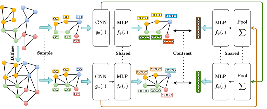
Figure 1: The proposed model for contrastive multi-view representation learning on both node and graph levels. A graph diffusion is used to generate an additional structural view of a sample graph which along with a regular view are sub-sampled and fed to two dedicated GNNs followed by a shared MLP to learn node representations. The learned features are then fed to a graph pooling layer followed by a shared MLP to learn graph representations. A discriminator contrasts node representations from one view with graph representation of another view and vice versa, and scores the agreement between representations which is used as the training signal.

3 Method

Inspired by recent advances in multi-view contrastive learning for visual representation learning, our approach learns node and graph representations by maximizing MI between node representations of one view and graph representation of another view and vice versa which achieves better results compared to contrasting global or multi-scale encodings on both node and graph classification tasks (see section 4.4). As shown in Figure 1, our method consists of the following components:

• An augmentation mechanism that transforms a sample graph into a correlated view of the same graph. We only apply the augmentation to the structure of the graphs and not the initial node features. This is followed by a sampler that sub-samples identical nodes from both views, i.e., similar to cropping in visual domain.

• Two dedicated GNNs, i.e., graph encoders, one for each view, followed by a shared MLP, i.e., projection head, to learn node representations for both views.

• A graph pooling layer, i.e., readout function, followed by a shared MLP, i.e., projection head, to learn graph representations for both views.

• A discriminator that contrasts node representations from one view with graph representation from another view and vice versa, and scores the agreement between them.

3.1 Augmentations

Recent works in self-supervised visual representation learning suggest that contrasting congruent and incongruent views of images allows encoders to learn rich representations (Tian et al., 2019; Bachman et al., 2019). Unlike images in which views are generated by standard augmentations, e.g., cropping, rotating, distorting colors, etc., defining views on graphs is not a trivial task. We can consider two types of augmentations on graphs: (1) feature-space augmentations operating on initial node features, e.g., masking or adding Gaussian noise, and (2) structure-space augmentations and corruptions operating on graph structure by adding or removing connectivities, sub-sampling, or generating global views using shortest distances or diffusion matrices. The former augmentation can be problematic as many benchmarks do not carry initial node features. Moreover, we observed that masking or adding noise on either spaces degrades the performance. Hence, we opted for generating a global view followed by sub-sampling.

We empirically show that in most cases the best results are achieved by transforming an adjacency matrix to a diffusion matrix and treating the two matrices as two congruent views of the same graph’s structure (see section 4.4). We speculate that because adjacency and diffusion matrices provide local and global views of a graph structure, respectively, maximizing agreement between representation learned from these two views allows the model to simultaneously encode rich local and global information.

Diffusion is formulated as Eq. (1) where $\textbf{T}\in\mathbb{R}^{n\times n}$ is the generalized transition matrix and $\Theta$ is the weighting coefficient which determines the ratio of global-local information. Imposing $\sum_{k=0}^{\infty}\theta_{k}=1$, $\theta_{k}\in[0,1]$, and $\lambda_{i}\in[0,1]$ where $\lambda_{i}$ are eigenvalues of T, guarantees convergence. Diffusion is computed once using fast approximation and sparsification methods (Klicpera et al., 2019b).

$$\textbf{S}=\sum_{k=0}^{\infty}{\Theta_{k}\textbf{T}^{k}}\in\mathbb{R}^{n\times n}$$ (1)

Given an adjacency matrix $\textbf{A}\in\mathbb{R}^{n\times n}$ and a diagonal degree matrix $\textbf{D}\in\mathbb{R}^{n\times n}$, Personalized PageRank (PPR) (Page et al., 1999) and heat kernel (Kondor & Lafferty, 2002), i.e., two instantiations of the generalized graph diffusion, are defined by setting $\mathbf{T}=\textbf{AD}^{-1}$, and $\theta_{k}=\alpha(1-\alpha)^{k}$ and $\theta_{k}=e^{-t}t^{k}/{k!}$, respectively, where $\alpha$ denotes teleport probability in a random walk and $t$ is diffusion time (Klicpera et al., 2019b). Closed-form solutions to heat and PPR diffusion are formulated in Eq. (2) and (3), respectively.

$$\textbf{S}^{\text{heat}}=\text{exp}\left({t\textbf{A}\textbf{D}^{-1}-t}\right)$$ (2)

$$\textbf{S}^{\text{PPR}}=\alpha\left(\textbf{I}_{n}-(1-\alpha)\textbf{D}^{-1/2}\textbf{A}\textbf{D}^{-1/2}\right)^{-1}$$ (3)

For sub-sampling, we randomly sample nodes and their edges from one view and select the exact nodes and edges from the other view. This procedure allows our approach to be applied to inductive tasks with graphs that do not fit into the GPU memory and also to transductive tasks by considering sub-samples as independent graphs.

3.2 Encoders

Our framework allows various choices of the network architecture without any constraints. We opt for simplicity and adopt the commonly used graph convolution network (GCN) (Kipf & Welling, 2017) as our base graph encoders. As shown in Figure 1, we use a dedicated graph encoder for each view, i.e., $g_{\theta}(.),g_{\omega}(.):\mathbb{R}^{n\times d_{x}}\times\mathbb{R}^{n\times n}\longmapsto\mathbb{R}^{n\times d_{h}}$. We consider adjacency and diffusion matrices as two congruent structural views and define GCN layers as $\sigma(\mathbf{\tilde{A}}\mathbf{X}\mathbf{\Theta})$ and $\sigma\big{(}\mathbf{S}\mathbf{X}\mathbf{\Theta}\big{)}$to learn two sets of node representations each corresponding to one of the views, respectively. $\mathbf{\tilde{A}}=\mathbf{\hat{D}}^{-1/2}\mathbf{\hat{A}}\mathbf{\hat{D}}^{-1/2}\in\mathbb{R}^{n\times n}$ is symmetrically normalized adjacency matrix, $\mathbf{\hat{D}}\in\mathbb{R}^{n\times n}$ is the degree matrix of $\mathbf{\hat{A}}=\mathbf{A}+\mathbf{I_{N}}$ where $\mathbf{I_{N}}$ is the identity matrix, $\textbf{S}\in\mathbb{R}^{n\times n}$ is diffusion matrix, $\textbf{X}\in\mathbb{R}^{n\times d_{x}}$ is the initial node features, $\mathbf{\Theta}\in\mathbb{R}^{d_{x}\times d_{h}}$ is network parameters, and $\sigma$ is a parametric ReLU (PReLU) non-linearity (He et al., 2015). The learned representations are then fed into a shared projection head $f_{\psi}(.):\mathbb{R}^{n\times d_{h}}\longmapsto\mathbb{R}^{n\times d_{h}}$ which is an MLP with two hidden layers and PReLU non-linearity. This results in two sets of node representations $\mathbf{H}^{\alpha}$, $\mathbf{H}^{\beta}\in\mathbb{R}^{n\times d_{h}}$ corresponding to two congruent views of a same graph.

For each view, we aggregate the node representations learned by GNNs, i.e., before the projection head, into a graph representation using a graph pooling (readout) function $\mathcal{P}(.):\mathbb{R}^{n\times d_{h}}\longmapsto\mathbb{R}^{d_{h}}$. We use a readout function similar to jumping knowledge network (JK-Net) (Xu et al., 2018) where we concatenate the summation of the node representations in each GCN layer and then feed them to a single layer feed-forward network to have a consistent dimension size between node and graph representations:

$$\vec{h}_{g}=\sigma\left({\operatorname*{\parallel}_{l=1}^{L}\left[\sum_{i=1}^{n}\vec{h}_{i}^{(l)}\right]}\mathbf{W}\right)\in\mathbb{R}^{h_{d}}$$ (4)

where $\vec{h}_{i}^{(l)}$ is the latent representation of node $i$ in layer $l$, $||$ is the concatenation operator, $L$ is the number of GCN layers, $\mathbf{W}\in\mathbb{R}^{(L\times d_{h})\times d_{h}}$ is the network parameters, and $\sigma$ is a PReLU non-linearity. In section 4.4, we show that this pooling function achieves better results compared to more complicated graph pooling methods such as DiffPool (Ying et al., 2018). Applying the readout function to node representations results in two graph representations, each associated with one of the views. The representations are then fed into a shared projection head $f_{\phi}(.):\mathbb{R}^{d_{h}}\longmapsto\mathbb{R}^{d_{h}}$, which is an MLP with two hidden layers and PReLU non-linearity, resulting in the final graph representations: $\vec{h}_{g}^{\alpha},\vec{h}_{g}^{\beta}\in\mathbb{R}^{d_{h}}$.

At inference time, we aggregate the representations from both views in both node and graph levels by summing them up: $\vec{h}=\vec{h}_{g}^{\alpha}+\vec{h}_{g}^{\beta}\in\mathbb{R}^{n}$ and $\mathbf{H}=\mathbf{H}^{\alpha}+\mathbf{H}^{\beta}\in\mathbb{R}^{n\times d_{h}}$ and return them as graph and node representations, respectively, for the down-stream tasks.

3.3 Training

In order to train the encoders end-to-end and learn rich node and graph level representations that are agnostic to down-stream tasks, we utilize the deep InfoMax (Hjelm et al., 2019) approach and maximize the MI between two views by contrasting node representations of one view with graph representation of the other view and vice versa. We empirically show that this approach consistently outperforms contrasting graph-graph or multi-scale encodings on both node and graph classifications benchmarks (see section 4.4). We define the objective as follows:

$$\max_{\theta,\omega,\phi,\psi}\frac{1}{|\mathcal{G}|}\sum_{g\in\mathcal{G}}\left[\frac{1}{|g|}\sum_{i=1}^{|g|}\left[\text{MI}\left(\vec{h}_{i}^{\alpha},\vec{h}_{g}^{\beta}\right)+\text{MI}\left(\vec{h}_{i}^{\beta},\vec{h}_{g}^{\alpha}\right)\right]\right]$$ (5)

where ${\theta,\omega,\phi,\psi}$ are graph encoder and projection head parameters, ${|\mathcal{G}|}$ is the number of graphs in train set or number of sub-sampled graphs in transductive setting, ${|g|}$ is the number of nodes in graph $g$, and $\vec{h}_{i}^{\alpha},\vec{h}_{g}^{\beta}$ are representations of node $i$ and graph $g$ encoded from views $\alpha,\beta$, respectively.

MI is modeled as discriminator $\mathcal{D}(.,.):\mathbb{R}^{d_{h}}\times\mathbb{R}^{d_{h}}\longmapsto\mathbb{R}$ that takes in a node representation from one view and a graph representation from another view, and scores the agreement between them. We simply implement the discriminator as the dot product between two representations: $\mathcal{D}(\vec{h}_{n},\vec{h}_{g})=\vec{h}_{n}.\vec{h}_{g}^{T}$. We observed a slight improvement in node classification benchmarks when discriminator and projection heads are integrated into a bilinear layer. In order to decide the MI estimator, we investigate four estimators and chose the best one for each benchmark (see section 4.4).

We provide the positive samples from joint distribution $x_{p}\sim p\left(\left[\mathbf{X},\tau_{\alpha}\left(\mathbf{A}\right)\right],\left[\mathbf{X},\tau_{\beta}\left(\mathbf{A}\right)\right]\right)$ and the negative samples from the product of marginals $x_{n}\sim p\left(\left[\mathbf{X},\tau_{\alpha}(\mathbf{A}\right)\right])p(\left[\mathbf{X},\tau_{\beta}\left(\mathbf{A}\right)\right])$. To generate negative samples in transductive tasks, we randomly shuffle the features (Veličković et al., 2019). Finally, we optimize the model parameters with respect to the objective using mini-batch stochastic gradient descent. Assuming a set of training graphs $\mathcal{G}$ where a sample graph $g=(\textbf{A},\textbf{X})\in\mathcal{G}$ consists of an adjacency matrix $\textbf{A}\in\{0,1\}^{n\times n}$ and initial node features $\textbf{X}\in\mathbb{R}^{n\times d_{x}}$, our proposed multi-view representation learning algorithm is summarized as follows:

Input: Augmentations $\tau_{\alpha}$ and $\tau_{\beta}$, sampler $\Gamma$, pooling $\mathcal{P}$, discriminator $\mathcal{D}$, loss $\mathcal{L}$, encoders $g_{\theta}$, $g_{\omega}$, $f_{\psi}$, $f_{\phi}$, and training graphs $\{\mathcal{G}|g=(\mathbf{X},\mathbf{A})\in\mathcal{G}\}$

for sampled batch $\{g_{k}\}_{k=1}^{N}\in\mathcal{G}$ do

       // compute encodings: for $k=1$ to $N$ do

             $\mathbf{X}_{k},\mathbf{A}_{k}=\Gamma(g_{k})$

              // sub-sample graph$\mathbf{V}_{k}^{\alpha}=\tau_{\alpha}\left(\mathbf{A}_{k}\right)$

              // first view$\mathbf{Z}^{\alpha}_{k}=g_{\theta}\left(\mathbf{X}_{k},\mathbf{V}_{k}^{\alpha}\right)$

              // node rep.$\mathbf{H}^{\alpha}_{k}=f_{\psi}\left(\mathbf{Z}^{\alpha}_{k}\right)$

              // projected node rep.$\vec{h}_{k}^{\alpha}=f_{\phi}\left(\mathcal{P}\left(\mathbf{Z}^{\alpha}_{k}\right)\right)$

              // projected graph rep.$\mathbf{V}_{k}^{\beta}=\tau_{\beta}\left(\mathbf{A}_{k}\right)$

              // second view$\mathbf{Z}^{\beta}_{k}=g_{\omega}\left(\mathbf{X}_{k},\mathbf{V}_{k}^{\beta}\right)$

              // node rep.$\mathbf{H}^{\beta}_{k}=f_{\psi}\left(\mathbf{Z}^{\beta}_{k}\right)$

              // projected node rep.$\vec{h}_{k}^{\beta}=f_{\phi}\left(\mathcal{P}\left(\mathbf{Z}^{\beta}_{k}\right)\right)$

              // projected graph rep.

       end for

      // compute pairwise similarity: for $i=1$ to $N$ and $j=1$ to $N$ do

             $s_{ij}^{\alpha}=\mathcal{D}\left(\vec{h}_{i}^{\alpha},\mathbf{H}^{\beta}_{j}\right)$, $s_{ij}^{\beta}=\mathcal{D}\left(\vec{h}_{i}^{\beta},\mathbf{H}^{\alpha}_{j}\right)$

       end for

      // compute gradients: $\bigtriangledown_{\theta,\omega,\phi,\psi}\frac{1}{N^{2}}\sum\limits_{i=1}^{N}\sum\limits_{j=1}^{N}{\left[\mathcal{L}\left(s_{ij}^{\alpha}\right)+\mathcal{L}\left(s_{ij}^{\beta}\right)\right]}$

end for

return $\left[\mathbf{H}^{\alpha}_{g}+\mathbf{H}^{\beta}_{g},\vec{h}_{g}^{\alpha}+\vec{h}_{g}^{\beta}\right]$, $\forall g\in\mathcal{G}$

Algorithm 1 Contrastive multi-view graph representation learning algorithm.

4 Experimental Results

Table 1: Statistics of classification benchmarks.

	Node			Graph
	cora	citeseer	pubmed	mutag	ptc-mr	imdb-bin	imdb-multi	reddit-bin
$|$ Graphs$|$	1	1	1	188	344	1000	1500	2000
$|$ Nodes$|$	3,327	2,708	19,717	17.93	14.29	19.77	13.0	508.52
$|$ Edges$|$	4,732	5,429	44,338	19.79	14.69	193.06	65.93	497.75
$|$ Classes$|$	6	7	3	2	2	2	3	2

Table 2: Mean node classification accuracy for supervised and unsupervised models. The input column highlights the data available to each model during training (X: features, A: adjacency matrix, S: diffusion matrix, Y: labels).

method		input	cora	citeseer	pubmed
supervised	MLP (Veličković et al., 2018)	X, Y	55.1	46.5	71.4
	ICA (Lu & Getoor, 2003)	A, Y	75.1	69.1	73.9
	LP (Zhu et al., 2003)	A, Y	68.0	45.3	63.0
	ManiReg (Belkin et al., 2006)	X, A, Y	59.5	60.1	70.7
	SemiEmb (Weston et al., 2012)	X, Y	59.0	59.6	71.7
	Planetoid (Yang et al., 2016)	X, Y	75.7	64.7	77.2
	Chebyshev (Defferrard et al., 2016)	X, A, Y	81.2	69.8	74.4
	GCN (Kipf & Welling, 2017)	X, A, Y	81.5	70.3	79.0
	MoNet (Monti et al., 2017)	X, A, Y	81.7 $\pm$ 0.5	$-$	78.8 $\pm$ 0.3
	JKNet (Xu et al., 2018)	X, A, Y	82.7 $\pm$ 0.4	73.0 $\pm$ 0.5	77.9 $\pm$ 0.4
	GAT (Veličković et al., 2018)	X, A, Y	83.0 $\pm$ 0.7	72.5 $\pm$ 0.7	79.0 $\pm$ 0.3
unsupervised	Linear (Veličković et al., 2019)	X	47.9 $\pm$ 0.4	49.3 $\pm$ 0.2	69.1 $\pm$ 0.3
	DeepWalk (Perozzi et al., 2014)	X, A	70.7 $\pm$ 0.6	51.4 $\pm$ 0.5	74.3 $\pm$ 0.9
	GAE (Kipf & Welling, 2016)	X, A	71.5 $\pm$ 0.4	65.8 $\pm$ 0.4	72.1 $\pm$ 0.5
	VERSE (Tsitsulin et al., 2018)	X, S, A	72.5 $\pm$ 0.3	55.5 $\pm$ 0.4	$-$
	DGI (Veličković et al., 2019)	X, A	82.3 $\pm$ 0.6	71.8 $\pm$ 0.7	76.8 $\pm$ 0.6
	DGI (Veličković et al., 2019)	X, S	83.8 $\pm$ 0.5	72.0 $\pm$ 0.6	77.9 $\pm$ 0.3
	Ours	X, S, A	86.8 $\pm$ 0.5	73.3 $\pm$ 0.5	80.1 $\pm$ 0.7

Table 3: Performance on node clustering task reported in normalized MI (NMI) and adjusted rand index (ARI) measures.

method		cora		citeseer		pubmed
		NMI	ARI	NMI	ARI	NMI	ARI
unsupervised	VGAE (Kipf & Welling, 2016)	0.3292	0.2547	0.2605	0.2056	0.3108	0.3018
	MGAE (Wang et al., 2017)	0.5111	0.4447	0.4122	0.4137	0.2822	0.2483
	ARGA (Pan et al., 2018)	0.4490	0.3520	0.3500	0.3410	0.2757	0.2910
	ARVGA (Pan et al., 2018)	0.4500	0.3740	0.2610	0.2450	0.1169	0.0777
	GALA (Park et al., 2019)	0.5767	0.5315	0.4411	0.4460	0.3273	0.3214
	Ours	0.6291	0.5696	0.4696	0.4497	0.3609	0.3386

Table 4: Mean 10-fold cross validation accuracy on graphs for kernel, supervised, and unsupervised methods.

method		mutag	ptc-mr	imdb-bin	imdb-multi	reddit-bin
Kernel	SP (Borgwardt & Kriegel, 2005)	85.2 $\pm$ 2.4	58.2 $\pm$ 2.4	55.6 $\pm$ 0.2	38.0 $\pm$ 0.3	64.1 $\pm$ 0.1
	GK (Shervashidze et al., 2009)	81.7 $\pm$ 2.1	57.3 $\pm$ 1.4	65.9 $\pm$ 1.0	43.9 $\pm$ 0.4	77.3 $\pm$ 0.2
	WL (Shervashidze et al., 2011)	80.7 $\pm$ 3.0	58.0 $\pm$ 0.5	72.3 $\pm$ 3.4	47.0 $\pm$ 0.5	68.8 $\pm$ 0.4
	DGK (Yanardag & Vishwana, 2015)	87.4 $\pm$ 2.7	60.1 $\pm$ 2.6	67.0 $\pm$ 0.6	44.6 $\pm$ 0.5	78.0 $\pm$ 0.4
	MLG (Kondor & Pan, 2016)	87.9 $\pm$ 1.6	63.3 $\pm$ 1.5	66.6 $\pm$ 0.3	41.2 $\pm$ 0.0	$-$
supervised	GraphSAGE (Hamilton et al., 2017)	85.1 $\pm$ 7.6	63.9 $\pm$ 7.7	72.3 $\pm$ 5.3	50.9 $\pm$ 2.2	$–$
	GCN (Kipf & Welling, 2017)	85.6 $\pm$ 5.8	64.2 $\pm$ 4.3	74.0 $\pm$ 3.4	51.9 $\pm$ 3.8	50.0 $\pm$ 0.0
	GIN-0 (Xu et al., 2019b)	89.4 $\pm$ 5.6	64.6 $\pm$ 7.0	75.1 $\pm$ 5.1	52.3 $\pm$ 2.8	92.4 $\pm$ 2.5
	GIN-$\epsilon$ (Xu et al., 2019b)	89.0 $\pm$ 6.0	63.7 $\pm$ 8.2	74.3 $\pm$ 5.1	52.1 $\pm$ 3.6	92.2 $\pm$ 2.3
	GAT (Veličković et al., 2018)	89.4 $\pm$ 6.1	66.7 $\pm$ 5.1	70.5 $\pm$ 2.3	47.8 $\pm$ 3.1	85.2 $\pm$ 3.3
unsupervised	random walk (Gärtner et al., 2003)	83.7 $\pm$ 1.5	57.9 $\pm$ 1.3	50.7 $\pm$ 0.3	34.7 $\pm$ 0.2	$-$
	node2vec (Grover & Leskovec, 2016)	72.6 $\pm$ 10.2	58.6 $\pm$ 8.0	$-$	$-$	$-$
	sub2vec (Adhikari et al., 2018)	61.1 $\pm$ 15.8	60.0 $\pm$ 6.4	55.3 $\pm$ 1.5	36.7 $\pm$ 0.8	71.5 $\pm$ 0.4
	graph2vec (Narayanan et al., 2017)	83.2 $\pm$ 9.6	60.2 $\pm$ 6.9	71.1 $\pm$ 0.5	50.4 $\pm$ 0.9	75.8 $\pm$ 1.0
	InfoGraph (Sun et al., 2020)	89.0 $\pm$ 1.1	61.7 $\pm$ 1.4	73.0 $\pm$ 0.9	49.7 $\pm$ 0.5	82.5 $\pm$ 1.4
	Ours	89.7 $\pm$ 1.1	62.5 $\pm$ 1.7	74.2 $\pm$ 0.7	51.2 $\pm$ 0.5	84.5 $\pm$ 0.6

4.1 Benchmarks

We use three node classification and five graph classification benchmarks widely used in the literature (Kipf & Welling, 2017; Veličković et al., 2018, 2019; Sun et al., 2020). For node classification, we use Citeseer, Cora, and Pubmed citation networks (Sen et al., 2008) where documents (nodes) are connected through citations (edges). For graph classification, we use the following: MUTAG (Kriege & Mutzel, 2012) containing mutagenic compounds, PTC (Kriege & Mutzel, 2012) containing compounds tested for carcinogenicity, Reddit-Binary (Yanardag & Vishwana, 2015) connecting users (nodes) through responses (edges) in Reddit online discussions, and IMDB-Binary and IMDB-Multi (Yanardag & Vishwana, 2015) connecting actors/actresses (nodes) based on movie appearances (edges). The statistics are summarized in Table 1.

4.2 Evaluation Protocol

For both node and graph classification benchmarks, we evaluate the proposed approach under the linear evaluation protocol and for each task, we closely follow the experimental protocol of the previous state-of-the-art approaches. For node classification, we follow DGI and report the mean classification accuracy with standard deviation on the test nodes after 50 runs of training followed by a linear model. For graph classification, we follow InfoGraph and report the mean 10-fold cross validation accuracy with standard deviation after 5 runs followed by a linear SVM. The linear classifier is trained using cross validation on training folds of data and the best mean classification accuracy is reported. Moreover, for node classification benchmarks, we evaluate the proposed method under clustering evaluation protocol and cluster the learned representations using K-Means algorithm. Similar to (Park et al., 2019), we set the number of clusters to the number of ground-truth classes and report the average normalized MI (NMI) and adjusted rand index (ARI) for 50 runs.

We initialize the parameters using Xavier initialization (Glorot & Bengio, 2010) and train the model using Adam optimizer (Kingma & Ba, 2014) with an initial learning rate of 0.001. To have fair comparisons, we follow InfoGraph for graph classification and choose the number of GCN layers, number of epochs, batch size, and the C parameter of the SVM from [2, 4, 8, 12], [10, 20, 40, 100], [32, 64, 128, 256], and $[10^{-3}$, $10^{-2}$, …, $10^{2}$, $10^{3}$], respectively. For node classification, we follow DGI and set the number of GCN layers and the number of epochs and to 1 and 2,000, respectively, and choose the batch size from [2, 4, 8]. We also use early stopping with a patience of 20. Finally, we set the size of hidden dimension of both node and graph representations to 512. For chosen hyper-parameters see Appendix.

4.3 Comparison with State-of-the-Art

To evaluate node classification under the linear evaluation protocol, we compare our results with unsupervised models including DeepWalk (Perozzi et al., 2014) and DGI. We also train a GAE (Kipf & Welling, 2016), a variant of DGI with a GDC encoder, and a variant of VERSE (Tsitsulin et al., 2018) by minimizing KL-divergence between node representations and diffusion matrix. Furthermore, we compare our results with supervised models including an MLP, iterative classification algorithm (ICA) (Lu & Getoor, 2003), label propagation (LP) (Zhu et al., 2003), manifold regularization (ManiReg) (Belkin et al., 2006), semi-supervised embedding (SemiEmb) (Weston et al., 2012), Planetoid (Yang et al., 2016), Chebyshev (Defferrard et al., 2016), mixture model networks (MoNet) (Monti et al., 2017), JK-Net, GCN, and GAT. The results reported in Table 2 show that we achieve state-of-the-art results with respect to previous unsupervised models. For example, on Cora, we achieve 86.8% accuracy, which is a 5.5% relative improvement over previous state-of-the-art. When compared to supervised baselines, we outperform strong supervised baselines: on Cora and PubMed benchmarks we observe 4.5% and 1.4% relative improvement over GAT, respectively.

To evaluate node classification under the clustering protocol, we compare our model with models reported in (Park et al., 2019) including: variational GAE (VGAE) (Kipf & Welling, 2016), marginalized GAE (MGAE) (Wang et al., 2017), adversarially regularized GAE (ARGA) and VGAE (ARVGA) (Pan et al., 2018), and GALA (Park et al., 2019). The results shown in Table 3 suggest that our model achieves state-of-the-art NMI and ARI scores across all benchmarks.

To evaluate graph classification under the linear evaluation protocol, we compare our results with five graph kernel methods including shortest path kernel (SP) (Borgwardt & Kriegel, 2005), Graphlet kernel (GK) (Shervashidze et al., 2009), Weisfeiler-Lehman sub-tree kernel (WL) (Shervashidze et al., 2011), deep graph kernels (DGK) (Yanardag & Vishwana, 2015), and multi-scale Laplacian kernel (MLG) (Kondor & Pan, 2016) reported in (Sun et al., 2020). We also compare with five supervised GNNs reported in (Xu et al., 2019b) including GraphSAGE (Hamilton et al., 2017), GCN, GAT, and two variants of GIN: GIN-0 and GIN-$\epsilon$. Finally, We compare the results with five unsupervised methods including random walk (Gärtner et al., 2003), node2vec (Grover & Leskovec, 2016), sub2vec (Adhikari et al., 2018), graph2vec (Narayanan et al., 2017), and InfoGraph. The results shown in Table 4 suggest that our approach achieves state-of-the-art results with respect to unsupervised models. For example, on Reddit-Binary (Yanardag & Vishwana, 2015), it achieves 84.5% accuracy, i.e., a 2.4% relative improvement over previous state-of-the-art. Our model also outperforms kernel methods in 4 out of 5 datasets and also outperforms best supervised model in one of the datasets. When compared to supervised baselines individually, our model outperforms GCN and GAT models in 3 out of 5 datasets, e.g., a 5.3% relative improvement over GAT on IMDB-Binary dataset.

It is noteworthy that we achieve the state-of-the-art results on both node and graph classification benchmarks using a unified approach and unlike previous unsupervised models (Veličković et al., 2019; Sun et al., 2020), we do not devise a specialized encoder for each task.

4.4 Ablation Study

Table 5: Effect of MI estimator, contrastive mode, and views on the accuracy on both node and graph classification tasks.

		Node			Graph
		cora	citeseer	pubmed	mutag	ptc-mr	imdb-bin	imdb-multi	reddit-bin
MI Est.	NCE	85.8 $\pm$ 0.7	73.3 $\pm$ 0.5	80.1 $\pm$ 0.7	82.2 $\pm$ 3.2	54.6 $\pm$ 2.5	73.7 $\pm$ 0.5	50.8 $\pm$ 0.8	79.7 $\pm$ 2.2
	JSD	86.7 $\pm$ 0.6	72.9 $\pm$ 0.6	79.4 $\pm$ 1.0	89.7 $\pm$ 1.1	62.5 $\pm$ 1.7	74.2 $\pm$ 0.7	51.1 $\pm$ 0.5	84.5 $\pm$ 0.6
	NT-Xent	86.8 $\pm$ 0.5	72.9 $\pm$ 0.6	79.3 $\pm$ 0.8	75.4 $\pm$ 7.8	51.2 $\pm$ 3.3	63.6 $\pm$ 4.2	50.4 $\pm$ 0.6	82.0 $\pm$ 1.1
	DV	85.4 $\pm$ 0.6	73.3 $\pm$ 0.5	78.9 $\pm$ 0.8	83.4 $\pm$ 1.9	56.7 $\pm$ 2.5	72.5 $\pm$ 0.8	51.1 $\pm$ 0.5	76.3 $\pm$ 5.6
Mode	local-global	86.8 $\pm$ 0.5	73.3 $\pm$ 0.5	80.1 $\pm$ 0.7	89.7 $\pm$ 1.1	62.5 $\pm$ 1.7	74.2 $\pm$ 0.7	51.1 $\pm$ 0.5	84.5 $\pm$ 0.6
	global	$-$	$-$	$-$	85.4 $\pm$ 2.8	56.0 $\pm$ 2.1	72.4 $\pm$ 0.4	49.7 $\pm$ 0.8	80.8 $\pm$ 1.8
	Multi-scale	83.2 $\pm$ 0.9	63.5 $\pm$ 1.5	75.7 $\pm$ 1.1	88.0 $\pm$ 0.8	56.6 $\pm$ 1.8	72.7 $\pm$ 0.4	50.6 $\pm$ 0.5	82.8 $\pm$ 0.6
	Hybrid	$-$	$-$	$-$	86.1 $\pm$ 1.7	56.1 $\pm$ 1.4	73.3 $\pm$ 1.2	49.6 $\pm$ 0.6	78.2 $\pm$ 4.2
	Ensemble	86.2 $\pm$ 0.6	73.3 $\pm$ 0.5	79.7 $\pm$ 0.9	82.5 $\pm$ 1.9	54.0 $\pm$ 3.0	73.0 $\pm$ 0.4	49.9 $\pm$ 0.9	81.4 $\pm$ 1.8
Views	Adj-ppr	86.8 $\pm$ 0.5	73.3 $\pm$ 0.5	80.1 $\pm$ 0.7	89.7 $\pm$ 1.1	62.5 $\pm$ 1.7	74.2 $\pm$ 0.7	51.1 $\pm$ 0.5	84.5 $\pm$ 0.6
	Adj-heat	86.4 $\pm$ 0.5	71.8 $\pm$ 0.5	77.2 $\pm$ 1.2	85.0 $\pm$ 1.9	55.8 $\pm$ 1.1	72.8 $\pm$ 0.5	50.0 $\pm$ 0.6	81.6 $\pm$ 0.9
	Adj-dist	84.5 $\pm$ 0.6	72.7 $\pm$ 0.7	74.6 $\pm$ 1.4	87.1 $\pm$ 1.0	58.7 $\pm$ 2.2	72.0 $\pm$ 0.7	50.7 $\pm$ 0.6	81.8 $\pm$ 0.7
	ppr-heat	85.8 $\pm$ 0.5	72.9 $\pm$ 0.5	78.1 $\pm$ 0.9	87.7 $\pm$ 1.2	57.6 $\pm$ 1.6	72.2 $\pm$ 0.6	51.2 $\pm$ 0.8	82.3 $\pm$ 1.0
	ppr-dist	85.9 $\pm$ 0.5	73.2 $\pm$ 0.4	74.7 $\pm$ 1.2	87.1 $\pm$ 1.0	60.0 $\pm$ 2.5	72.4 $\pm$ 1.4	51.1 $\pm$ 0.8	82.5 $\pm$ 1.1
	heat-dist	85.2 $\pm$ 0.4	70.4 $\pm$ 0.7	72.8 $\pm$ 0.7	87.4 $\pm$ 1.2	58.6 $\pm$ 1.7	72.2 $\pm$ 0.6	50.5 $\pm$ 0.5	80.3 $\pm$ 0.6

4.4.1 Effect of Mutual Information Estimator

We investigated four MI estimators including: noise-contrastive estimation (NCE) (Gutmann & Hyvärinen, 2010; Oord et al., 2018), Jensen-Shannon (JSD) estimator following formulation in (Nowozin et al., 2016), normalized temperature-scaled cross-entropy (NT-Xent) (Chen et al., 2020), and Donsker-Varadhan (DV) representation of the KL-divergence (Donsker & Varadhan, 1975). The results shown in Table 5 suggests that Jensen-Shannon estimator achieves better results across all graph classification benchmarks, whereas in node classification benchmarks, NCE achieves better results in 2 out of 3 datasets.

4.4.2 Effect of Contrastive Mode

We considered five contrastive modes including: local-global, global-global, multi-scale, hybrid, and ensemble modes. In local-global mode we extend deep InfoMax (Hjelm et al., 2019) and contrast node encodings from one view with graph encodings from another view and vice versa. Global-global mode is similar to (Li et al., 2019; Tian et al., 2019; Chen et al., 2020) where we contrast graph encodings from different views. In multi-scale mode, we contrast graph encodings from one view with intermediate encodings from another view and vice versa, and we also contrast intermediate encodings from one view with node encodings from another view and vice versa. We use two DiffPool layers to compute the intermediate encodings. The first layer projects nodes into a set of clusters where the number of clusters, i.e., motifs, is set as 25% of the number of nodes before applying DiffPool, whereas the second layer projects the learned cluster encodings into a graph encoding. In hybrid mode, we use both local-global and global-global modes. Finally, in ensemble mode, we contrast nodes and graph encodings from a same view for all views.

Results reported in Table 5 suggest that contrasting node and graph encodings consistently perform better across benchmarks. The results also reveal important differences between graph and visual representation learning: (1) in visual representation learning, contrasting global views achieves best results (Tian et al., 2019; Chen et al., 2020), whereas for graphs, contrasting node and graph encodings achieves better performance for both node and graph classification tasks, and (2) contrasting multi-scale encodings helps visual representation learning (Bachman et al., 2019) but has a negative effect on graph representation learning.

4.4.3 Effect of Views

We investigated four structural views including adjacency matrix, PPR and heat diffusion matrices, and pair-wise distance matrix where adjacency conveys local information and the latter three capture global information. Adjacency matrix is processed into a symmetrically normalized adjacency matrix (see section 3.2), and PPR and heat diffusion matrices are computed using Eq. (3) and (2), respectively. The shortest pair-wise distance matrix is computed by Floyd-Warshall algorithm, inversed in an element-wise fashion, and row-normalized using softmax. All views are computed once in preprocessing. The results shown in Table 5 suggest that contrasting encodings from adjacency and PPR views performs better across the benchmarks.

Furthermore, we investigated whether increasing the number of views increases the performance on down-stream tasks, monotonically. Following (Tian et al., 2019), we extended number of views to three by anchoring the main view on adjacency matrix and considering two diffusion matrices as other views. The results (see Appendix) suggest that unlike visual representation learning, extending the views does not help. We speculate this is because different diffusion matrices carry similar information about the graph structure. We also followed (Chen et al., 2020) and randomly sampled 2 out of 4 views for each training sample in each mini-batch and contrasted the representation. We observed that unlike visual domain, it degraded the performance.

4.4.4 Negative Sampling & Regularization

We investigated the performance with respect to batch size where a batch of size $N$ consists of $N-1$ negative and 1 positive examples. We observed that in graph classification, increasing the batch size slightly improves the performance, whereas, in node classification, it does not have a significant effect. Thus we opted for efficient smaller batch sizes. To generate negative samples in node classification, we considered two corruption functions: (1) random feature permutation, and (2) adjacency matrix corruption. We observed that applying the former achieves significantly better results compared to the latter or a combination of both.

Furthermore, we observed that applying normalization layers such as BatchNorm (Ioffe & Szegedy, 2015) or LayerNorm (Ba et al., 2016), or regularization methods such as adding Gaussian noise, L2 regularization, or dropout (Srivastava et al., 2014) during the pre-training degrades the performance on down-stream tasks (except early stopping).

5 Conclusion

We introduced a self-supervised approach for learning node and graph level representations by contrasting encodings from two structural views of graphs including first-order neighbors and a graph diffusion. We showed that unlike visual representation learning, increasing the number of views or contrasting multi-scale encodings do not improve the performance. Using these findings, we achieved new state-of-the-art in self-supervised learning on 8 out of 8 node and graph classification benchmarks under the linear evaluation protocol and outperformed strong supervised baselines in 4 out of 8 benchmarks. In future work, we are planning to investigate large pre-training and transfer learning capabilities of the proposed method.

6 Appendix

6.1 Implementation Details

The model is implemented with PyTorch and each benchmark is run on a single GPU. For a given dataset, the node features are processed as follows. If the dataset contains initial node features, they are normalize using the standard score. If the dataset does not contains initial node features, but carries node labels, they are used as the initial node features (only in graph classification benchmarks). Otherwise, if the dataset has neither, the node features are initialized with node degrees. Diffusion and pair-wise distance matrices are computed once in preprocessing step using NetworkX and Numpy packages. The shortest pair-wise distance matrix is computed by Floyd-Warshall algorithm, inversed in an element-wise fashion, and row-normalized using softmax.

6.2 Hyper-Parameters

In out experiments, we fixed $\alpha$=0.2 and $t$=5 for PPR and heat diffusion, respectively. We used grid search to choose the hyper-parameters from the following ranges. For graph classification, we chose the number of GCN layers, number of epochs, batch size, and the C parameter of the SVM from [2, 4, 8, 12], [10, 20, 40, 100], [32, 64, 128, 256], and $[10^{-3}$, $10^{-2}$, …, $10^{2}$, $10^{3}$], respectively. For node classification, we set the number of GCN layers and the number of epochs and to 1 and 2,000, respectively, and choose the batch size from [2, 4, 8]. We also use early stopping with a patience of 20. Finally, we set the size of hidden dimension of both node and graph representations to 512. The selected parameters are reported in Table 6.

6.3 Effect of Number of Views

Furthermore, we investigated whether increasing the number of views increases the performance on down-stream tasks, monotonically. We extended number of views to three by anchoring the main view on adjacency matrix and considering two diffusion matrices, i.e, PPR and heat, as other views. The results shown in Table 7 suggest that unlike visual representation learning, extending the views does not improve the performance on the down-stream tasks. We speculate this is because different diffusion matrices carry similar information about the graph structure and hence using more of them does not introduce useful signals.

6.4 Effect of Pooling

In addition to mentioned sum pooling, we tried mean pooling and two variants of DiffPool: (1) DiffPool-1 where we use a single layer of DiffPool to aggregate all node representations into a single graph representation, and (2) DiffPool-2 where we use two DiffPool layers to compute the intermediate representations. The first layer projects nodes into a set of clusters, i.e., motifs, where the number of clusters is set as 25% of the number of nodes before applying DiffPool, whereas the second layer projects the learned cluster representations into a single graph representations. It is noteworthy that to train the model with Diffpool layers, we jointly optimize the contrastive loss with an auxiliary link prediction loss and an entropy regularization. The results shown in Table 6 suggest that sum pooling outperforms other pooling layers in 6 out of 8 benchmarks ,i.e., 5 out of 5 graph classification and 1 out if 3 node classification benchmarks. Also, results suggest that mean pooling achieves better results in 2 out of 3 node classification benchmarks.

6.5 Effect of Encoder

We also investigated the effect of assigning a dedicated encoder for each view or sharing an encoder across views. The results in Table 6 show that using a dedicated encoder for each view consistently achieves better results across all benchmarks. When using shared encoder, we also randomly sampled 2 out 4 views for each training sample in each mini-batch and contrasted the representation. We observed that unlike visual domain, it degraded the performance.

6.6 Effect of Negative Samples

Considering the importance of the number of negative samples in contrastive learning, we investigated the effect of batch size on the mode performance. For graph classification benchmarks, we used batch sizes of [16, 32, 64, 128, 256] and for classification benchmarks we evaluated batch sizes of [2, 4, 8]. As shown in Figure 2, we observe that increasing the batch size slightly increases the performance on graph classification task but has an negligible effect on the node classification.

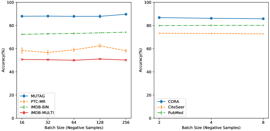
Figure 2: Effect of batch size (number of negative samples) on graph and node classification benchmarks. Increasing the batch size slightly increases the performance on graph classification task but has an negligible effect on the node classification.

Table 6: Summary of chosen hyper-parameters using grid search, and effect of graph pooling and encoders on the accuracy on both node and graph classification benchmarks. Using sum pooling and assigning dedicated encoders for each view achieve better results across the benchmarks.

		Node			Graph
		cora	citeseer	pubmed	mutag	ptc-mr	imdb-bin	imdb-multi	reddit-bin
Hyper	$|$Layers$|$	1	1	1	4	4	2	4	2
	$|$Batches$|$	2	2	2	20	40	20	40	20
	$|$Epochs$|$	2000	2000	2000	256	128	256	128	32
Pooling	sum	86.2 $\pm$ 0.6	73.3 $\pm$ 0.5	79.6 $\pm$ 0.9	89.7 $\pm$ 1.1	62.5 $\pm$ 1.7	74.2 $\pm$ 0.7	51.1 $\pm$ 0.5	84.5 $\pm$ 0.6
	mean	86.8 $\pm$ 0.5	73.2 $\pm$ 0.6	80.1 $\pm$ 0.7	88.8 $\pm$ 0.7	60.9 $\pm$ 1.2	72.3 $\pm$ 0.5	49.1 $\pm$ 0.7	79.4 $\pm$ 0.5
	diffpool-1	84.6 $\pm$ 0.8	65.2 $\pm$ 1.7	76.1 $\pm$ 0.8	89.6 $\pm$ 0.9	61.1 $\pm$ 0.2	72.8 $\pm$ 0.6	49.4 $\pm$ 0.9	81.3 $\pm$ 0.4
	diffpool-2	83.2 $\pm$ 0.9	63.5 $\pm$ 1.5	75.7 $\pm$ 1.1	88.0 $\pm$ 0.8	56.6 $\pm$ 1.8	72.7 $\pm$ 0.4	50.6 $\pm$ 0.5	82.8 $\pm$ 0.6
Enc.	shared	86.2 $\pm$ 0.6	72.8 $\pm$ 0.6	79.5 $\pm$ 0.1	82.8 $\pm$ 1.9	55.9 $\pm$ 2.2	73.0 $\pm$ 0.7	50.0 $\pm$ 0.3	81.3 $\pm$ 2.0
	dedicated	86.8 $\pm$ 0.5	73.3 $\pm$ 0.5	80.1 $\pm$ 0.7	89.7 $\pm$ 1.1	62.5 $\pm$ 1.7	74.2 $\pm$ 0.7	51.1 $\pm$ 0.5	84.5 $\pm$ 0.6

Table 7: Effect of number of views on node classification accuracy.

#Views	Cora	Citeseer	Pubmed
2	86.8 $\pm$ 0.5	73.3 $\pm$ 0.5	80.1 $\pm$ 0.7
3	85.3 $\pm$ 0.5	71.2 $\pm$ 0.7	79.9 $\pm$ 0.6

References

- Adhikari et al. (2018) Adhikari, B., Zhang, Y., Ramakrishnan, N., and Prakash, B. A. Sub2vec: Feature learning for subgraphs. In Pacific-Asia Conference on Knowledge Discovery and Data Mining, pp. 170–182, 2018.
- Ba et al. (2016) Ba, J. L., Kiros, J. R., and Hinton, G. E. Layer normalization. arXiv preprint arXiv:1607.06450, 2016.
- Bachman et al. (2019) Bachman, P., Hjelm, R. D., and Buchwalter, W. Learning representations by maximizing mutual information across views. In Advances in Neural Information Processing Systems, pp. 15509–15519, 2019.
- Belkin et al. (2006) Belkin, M., Niyogi, P., and Sindhwani, V. Manifold regularization: A geometric framework for learning from labeled and unlabeled examples. Journal of Machine Learning Research, 7:2399–2434, 2006.
- Borgwardt & Kriegel (2005) Borgwardt, K. M. and Kriegel, H.-P. Shortest-path kernels on graphs. In International Conference on Data Mining, 2005.
- Chen et al. (2020) Chen, T., Kornblith, S., Norouzi, M., and Hinton, G. A simple framework for contrastive learning of visual representations. arXiv preprint arXiv:2002.05709, 2020.
- Defferrard et al. (2016) Defferrard, M., Bresson, X., and Vandergheynst, P. Convolutional neural networks on graphs with fast localized spectral filtering. In Advances in Neural Information Processing Systems, pp. 3844–3852. 2016.
- Donsker & Varadhan (1975) Donsker, M. D. and Varadhan, S. S. Asymptotic evaluation of certain markov process expectations for large time. Communications on Pure and Applied Mathematics, 28(1):1–47, 1975.
- Duvenaud et al. (2015) Duvenaud, D. K., Maclaurin, D., Iparraguirre, J., Bombarell, R., Hirzel, T., Aspuru-Guzik, A., and Adams, R. P. Convolutional networks on graphs for learning molecular fingerprints. In Advances in Neural Information Processing Systems, pp. 2224–2232, 2015.
- Garcia Duran & Niepert (2017) Garcia Duran, A. and Niepert, M. Learning graph representations with embedding propagation. In Advances in Neural Information Processing Systems, pp. 5119–5130. 2017.
- Gärtner et al. (2003) Gärtner, T., Flach, P., and Wrobel, S. On graph kernels: Hardness results and efficient alternatives. In Learning theory and kernel machines, pp. 129–143. 2003.
- Gilmer et al. (2017) Gilmer, J., Schoenholz, S. S., Riley, P. F., Vinyals, O., and Dahl, G. E. Neural message passing for quantum chemistry. In International Conference on Machine Learning, pp. 1263–1272, 2017.
- Glorot & Bengio (2010) Glorot, X. and Bengio, Y. Understanding the difficulty of training deep feedforward neural networks. In International Conference on Artificial Intelligence and Statistics, pp. 249–256, 2010.
- Grover & Leskovec (2016) Grover, A. and Leskovec, J. node2vec: Scalable feature learning for networks. In International Conference on Knowledge Discovery and Data Mining, pp. 855–864, 2016.
- Gutmann & Hyvärinen (2010) Gutmann, M. and Hyvärinen, A. Noise-contrastive estimation: A new estimation principle for unnormalized statistical models. In International Conference on Artificial Intelligence and Statistics, pp. 297–304, 2010.
- Hamilton et al. (2017) Hamilton, W., Ying, Z., and Leskovec, J. Inductive representation learning on large graphs. In Advances in Neural Information Processing Systems, pp. 1024–1034, 2017.
- Hassani & Haley (2019) Hassani, K. and Haley, M. Unsupervised multi-task feature learning on point clouds. In International Conference on Computer Vision, pp. 8160–8171, 2019.
- He et al. (2015) He, K., Zhang, X., Ren, S., and Sun, J. Delving deep into rectifiers: Surpassing human-level performance on imagenet classification. In International Conference on Computer Vision, pp. 1026–1034, 2015.
- Hjelm et al. (2019) Hjelm, R. D., Fedorov, A., Lavoie-Marchildon, S., Grewal, K., Bachman, P., Trischler, A., and Bengio, Y. Learning deep representations by mutual information estimation and maximization. In International Conference on Learning Representations, 2019.
- Ioffe & Szegedy (2015) Ioffe, S. and Szegedy, C. Batch normalization: Accelerating deep network training by reducing internal covariate shift. In International Conference on Machine Learning, pp. 448–456, 2015.
- Jiang et al. (2019) Jiang, B., Lin, D., Tang, J., and Luo, B. Data representation and learning with graph diffusion-embedding networks. In Conference on Computer Vision and Pattern Recognition, pp. 10414–10423, 2019.
- Khasahmadi et al. (2020) Khasahmadi, A., Hassani, K., Moradi, P., Lee, L., and Morris, Q. Memory-based graph networks. In International Conference on Learning Representations, 2020.
- Kingma & Ba (2014) Kingma, D. P. and Ba, J. L. Adam: Amethod for stochastic optimization. In International Conference on Learning Representation, 2014.
- Kipf & Welling (2016) Kipf, T. N. and Welling, M. Variational graph auto-encoders. arXiv preprint arXiv:1611.07308, 2016.
- Kipf & Welling (2017) Kipf, T. N. and Welling, M. Semi-supervised classification with graph convolutional networks. In International Conference on Learning Representations, 2017.
- Klicpera et al. (2019a) Klicpera, J., Bojchevski, A., and Günnemann, S. Combining neural networks with personalized pagerank for classification on graphs. In International Conference on Learning Representations, 2019a.
- Klicpera et al. (2019b) Klicpera, J., Weiß enberger, S., and Günnemann, S. Diffusion improves graph learning. In Advances in Neural Information Processing Systems, pp. 13333–13345. 2019b.
- Kondor & Pan (2016) Kondor, R. and Pan, H. The multiscale laplacian graph kernel. In Advances in Neural Information Processing Systems, pp. 2990–2998. 2016.
- Kondor & Lafferty (2002) Kondor, R. I. and Lafferty, J. Diffusion kernels on graphs and other discrete structures. In International Conference on Machine Learning, pp. 315–22, 2002.
- Kriege & Mutzel (2012) Kriege, N. and Mutzel, P. Subgraph matching kernels for attributed graphs. In International Conference on Machine Learning, pp. 291–298, 2012.
- Kriege et al. (2016) Kriege, N. M., Giscard, P.-L., and Wilson, R. On valid optimal assignment kernels and applications to graph classification. In Advances in Neural Information Processing Systems, pp. 1623–1631, 2016.
- Li et al. (2015) Li, Y., Tarlow, D., Brockschmidt, M., and Zemel, R. Gated graph sequence neural networks. In International Conference on Learning Representations, 2015.
- Li et al. (2019) Li, Y., Gu, C., Dullien, T., Vinyals, O., and Kohli, P. Graph matching networks for learning the similarity of graph structured objects. In International Conference on Machine Learning, pp. 3835–3845, 2019.
- Linsker (1988) Linsker, R. Self-organization in a perceptual network. Computer, 21(3):105–117, 1988.
- Lu & Getoor (2003) Lu, Q. and Getoor, L. Link-based classification. In International Conference on Machine Learning, pp. 496–503, 2003.
- Monti et al. (2017) Monti, F., Boscaini, D., Masci, J., Rodola, E., Svoboda, J., and Bronstein, M. M. Geometric deep learning on graphs and manifolds using mixture model cnns. In Conference on Computer Vision and Pattern Recognition, 2017.
- Narayanan et al. (2017) Narayanan, A., Chandramohan, M., Venkatesan, R., Chen, L., Liu, Y., and Jaiswal, S. graph2vec: Learning distributed representations of graphs. arXiv preprint arXiv:1707.05005, 2017.
- Nowozin et al. (2016) Nowozin, S., Cseke, B., and Tomioka, R. f-gan: Training generative neural samplers using variational divergence minimization. In Advances in Neural Information Processing Systems, pp. 271–279. 2016.
- Oord et al. (2018) Oord, A. v. d., Li, Y., and Vinyals, O. Representation learning with contrastive predictive coding. arXiv preprint arXiv:1807.03748, 2018.
- Page et al. (1999) Page, L., Brin, S., Motwani, R., and Winograd, T. The pagerank citation ranking: Bringing order to the web. Technical report, Stanford InfoLab, 1999.
- Pan et al. (2018) Pan, S., Hu, R., Long, G., Jiang, J., Yao, L., and Zhang, C. Adversarially regularized graph autoencoder for graph embedding. In International Joint Conference on Artificial Intelligence, pp. 2609–2615, 2018.
- Park et al. (2019) Park, J., Lee, M., Chang, H. J., Lee, K., and Choi, J. Y. Symmetric graph convolutional autoencoder for unsupervised graph representation learning. In International Conference on Computer Vision, pp. 6519–6528, 2019.
- Perozzi et al. (2014) Perozzi, B., Al-Rfou, R., and Skiena, S. Deepwalk: Online learning of social representations. In International Conference on Knowledge Discovery and Data Mining, pp. 701–710, 2014.
- Ribeiro et al. (2017) Ribeiro, L., Saverese, P., and Figueiredo, D. Struc2vec: Learning node representations from structural identity. In International Conference on Knowledge Discovery and Data Mining, pp. 385–394, 2017.
- Sanchez-Gonzalez et al. (2018) Sanchez-Gonzalez, A., Heess, N., Springenberg, J. T., Merel, J., Riedmiller, M., Hadsell, R., and Battaglia, P. Graph networks as learnable physics engines for inference and control. In International Conference on Machine Learning, pp. 4470–4479, 2018.
- Sen et al. (2008) Sen, P., Namata, G., Bilgic, M., Getoor, L., Galligher, B., and Eliassi-Rad, T. Collective classification in network data. AI Magazine, 29(3):93–93, 2008.
- Shervashidze et al. (2009) Shervashidze, N., Vishwanathan, S., Petri, T., Mehlhorn, K., and Borgwardt, K. Efficient graphlet kernels for large graph comparison. In Artificial Intelligence and Statistics, pp. 488–495, 2009.
- Shervashidze et al. (2011) Shervashidze, N., Schweitzer, P., Leeuwen, E. J. v., Mehlhorn, K., and Borgwardt, K. M. Weisfeiler-lehman graph kernels. Journal of Machine Learning Research, 12:2539–2561, 2011.
- Srivastava et al. (2014) Srivastava, N., Hinton, G., Krizhevsky, A., Sutskever, I., and Salakhutdinov, R. Dropout: A simple way to prevent neural networks from overfitting. Journal of Machine Learning Research, 15(56):1929–1958, 2014.
- Sun et al. (2020) Sun, F.-Y., Hoffman, J., Verma, V., and Tang, J. Infograph: Unsupervised and semi-supervised graph-level representation learning via mutual information maximization. In International Conference on Learning Representations, 2020.
- Tang et al. (2015) Tang, J., Qu, M., Wang, M., Zhang, M., Yan, J., and Mei, Q. Line: Large-scale information network embedding. In International Conference on World Wide Web, pp. 1067–1077, 2015.
- Tian et al. (2019) Tian, Y., Krishnan, D., and Isola, P. Contrastive multiview coding. arXiv preprint arXiv:1906.05849, 2019.
- Tschannen et al. (2020) Tschannen, M., Djolonga, J., Rubenstein, P. K., Gelly, S., and Lucic, M. On mutual information maximization for representation learning. In International Conference on Learning Representations, 2020.
- Tsitsulin et al. (2018) Tsitsulin, A., Mottin, D., Karras, P., and Müller, E. Verse: Versatile graph embeddings from similarity measures. In International Conference on World Wide Web, pp. 539–548, 2018.
- Veličković et al. (2018) Veličković, P., Cucurull, G., Casanova, A., Romero, A., Liò, P., and Bengio, Y. Graph attention networks. In International Conference on Learning Representations, 2018.
- Veličković et al. (2019) Veličković, P., Fedus, W., Hamilton, W. L., Liò, P., Bengio, Y., and Hjelm, R. D. Deep graph infomax. In International Conference on Learning Representations, 2019.
- Vivona & Hassani (2019) Vivona, S. and Hassani, K. Relational graph representation learning for open-domain question answering. Advances in Neural Information Processing Systems, Graph Representation Learning Workshop, 2019.
- Wang et al. (2017) Wang, C., Pan, S., Long, G., Zhu, X., and Jiang, J. Mgae: Marginalized graph autoencoder for graph clustering. In Conference on Information and Knowledge Management, pp. 889–898, 2017.
- Wang et al. (2018) Wang, N., Zhang, Y., Li, Z., Fu, Y., Liu, W., and Jiang, Y.-G. Pixel2mesh: Generating 3d mesh models from single rgb images. In European Conference on Computer Vision, pp. 52–67, 2018.
- Wang et al. (2019) Wang, T., Zhou, Y., Fidler, S., and Ba, J. Neural graph evolution: Automatic robot design. In International Conference on Learning Representations, 2019.
- Weston et al. (2012) Weston, J., Ratle, F., Mobahi, H., and Collobert, R. Deep learning via semi-supervised embedding. In Neural Networks: Tricks of the Trade, pp. 639–655. 2012.
- Wu et al. (2020) Wu, Z., Pan, S., Chen, F., Long, G., Zhang, C., and Philip, S. Y. A comprehensive survey on graph neural networks. IEEE Transactions on Neural Networks and Learning Systems, 2020.
- Xu et al. (2019a) Xu, B., Shen, H., Cao, Q., Cen, K., and Cheng, X. Graph convolutional networks using heat kernel for semi-supervised learning. In International Joint Conference on Artificial Intelligence, pp. 1928–1934, 2019a.
- Xu et al. (2018) Xu, K., Li, C., Tian, Y., Sonobe, T., Kawarabayashi, K.-i., and Jegelka, S. Representation learning on graphs with jumping knowledge networks. In International Conference on Machine Learning, pp. 5453–5462, 2018.
- Xu et al. (2019b) Xu, K., Hu, W., Leskovec, J., and Jegelka, S. How powerful are graph neural networks? In International Conference on Learning Representations, 2019b.
- Yanardag & Vishwana (2015) Yanardag, P. and Vishwana, S. Deep graph kernels. In International Conference on Knowledge Discovery and Data Mining, pp. 1365–1374, 2015.
- Yang et al. (2016) Yang, Z., Cohen, W., and Salakhudinov, R. Revisiting semi-supervised learning with graph embeddings. In International Conference on Machine Learning, pp. 40–48, 2016.
- Ying et al. (2018) Ying, Z., You, J., Morris, C., Ren, X., Hamilton, W., and Leskovec, J. Hierarchical graph representation learning with differentiable pooling. In Advances in Neural Information Processing Systems, pp. 4800–4810, 2018.
- You et al. (2019) You, J., Ying, R., and Leskovec, J. Position-aware graph neural networks. In International Conference on Machine Learning, pp. 7134–7143, 2019.
- Zhang et al. (2020) Zhang, Z., Cui, P., and Zhu, W. Deep learning on graphs: A survey. IEEE Transactions on Knowledge and Data Engineering, 2020.
- Zhu et al. (2003) Zhu, X., Ghahramani, Z., and Lafferty, J. D. Semi-supervised learning using gaussian fields and harmonic functions. In International Conference on Machine Learning, pp. 912–919, 2003.