G. D. Alexeev
Joint Institute for Nuclear Research, 141980 Dubna, Moscow region, Russia
M. G. Alexeev
Department of Physics, University of Torino, 10125 Turin, Italy
Torino Section of INFN, 10125 Turin, Italy
A. Amoroso
Department of Physics, University of Torino, 10125 Turin, Italy
Torino Section of INFN, 10125 Turin, Italy
V. Andrieux
CERN, 1211 Geneva 23, Switzerland
Department of Physics, University of Illinois at Urbana-Champaign, Urbana, IL 61801-3080, USA
V. Anosov
Joint Institute for Nuclear Research, 141980 Dubna, Moscow region, Russia
A. Antoshkin
Joint Institute for Nuclear Research, 141980 Dubna, Moscow region, Russia
K. Augsten
Joint Institute for Nuclear Research, 141980 Dubna, Moscow region, Russia
Czech Technical University in Prague, 16636 Prague, Czech Republic
W. Augustyniak
National Centre for Nuclear Research, 02-093 Warsaw, Poland
C. D. R. Azevedo
Department of Physics, University of Aveiro, I3N, 3810-193 Aveiro, Portugal
B. Badełek
Faculty of Physics, University of Warsaw, 02-093 Warsaw, Poland
F. Balestra
Department of Physics, University of Torino, 10125 Turin, Italy
Torino Section of INFN, 10125 Turin, Italy
M. Ball
Helmholtz-Institut für Strahlen- und Kernphysik, Universität Bonn, 53115 Bonn, Germany
J. Barth
Helmholtz-Institut für Strahlen- und Kernphysik, Universität Bonn, 53115 Bonn, Germany
R. Beck
Helmholtz-Institut für Strahlen- und Kernphysik, Universität Bonn, 53115 Bonn, Germany
Y. Bedfer
IRFU, CEA, Université Paris-Saclay, 91191 Gif-sur-Yvette, France
J. Berenguer Antequera
Department of Physics, University of Torino, 10125 Turin, Italy
Torino Section of INFN, 10125 Turin, Italy
J. Bernhard
Institut für Kernphysik, Universität Mainz, 55099 Mainz, Germany
CERN, 1211 Geneva 23, Switzerland
M. Bodlak
Faculty of Mathematics and Physics, Charles University, 18000 Prague, Czech Republic
F. Bradamante
Trieste Section of INFN, 34127 Trieste, Italy
A. Bressan
Department of Physics, University of Trieste, 34127 Trieste, Italy
Trieste Section of INFN, 34127 Trieste, Italy
V. E. Burtsev
Tomsk Polytechnic University, 634050 Tomsk, Russia
W.-C. Chang
Academia Sinica, Institute of Physics, Taipei 11529, Taiwan
C. Chatterjee
Department of Physics, University of Trieste, 34127 Trieste, Italy
Trieste Section of INFN, 34127 Trieste, Italy
M. Chiosso
Department of Physics, University of Torino, 10125 Turin, Italy
Torino Section of INFN, 10125 Turin, Italy
A. G. Chumakov
Tomsk Polytechnic University, 634050 Tomsk, Russia
S.-U. Chung
Also at: Department of Physics, Pusan National University, Busan 609-735, Republic of Korea and Physics Department,
Brookhaven National Laboratory, Upton, NY 11973, USA.
Physik Department, Technische Universität München, 85748 Garching, Germany
A. Cicuttin
Also at: Abdus Salam ICTP, 34151 Trieste, Italy.
Trieste Section of INFN, 34127 Trieste, Italy
P. M. M. Correia
Department of Physics, University of Aveiro, I3N, 3810-193 Aveiro, Portugal
M. L. Crespo
Also at: Abdus Salam ICTP, 34151 Trieste, Italy.
Trieste Section of INFN, 34127 Trieste, Italy
D. D’Ago
Department of Physics, University of Trieste, 34127 Trieste, Italy
Trieste Section of INFN, 34127 Trieste, Italy
S. Dalla Torre
Trieste Section of INFN, 34127 Trieste, Italy
S. S. Dasgupta
Matrivani Institute of Experimental Research & Education, Calcutta-700 030, India
S. Dasgupta
Trieste Section of INFN, 34127 Trieste, Italy
I. Denisenko
Joint Institute for Nuclear Research, 141980 Dubna, Moscow region, Russia
O. Yu. Denisov
Torino Section of INFN, 10125 Turin, Italy
S. V. Donskov
State Scientific Center Institute for High Energy Physics of National Research Center ”Kurchatov Institute”, 142281 Protvino, Russia
N. Doshita
Yamagata University, Yamagata 992-8510, Japan
Ch. Dreisbach
Physik Department, Technische Universität München, 85748 Garching, Germany
W. Dünnweber
Retired from Ludwig-Maximilian-Universität, München, Germany.
R. R. Dusaev
Tomsk Polytechnic University, 634050 Tomsk, Russia
A. Efremov
Deceased.
Joint Institute for Nuclear Research, 141980 Dubna, Moscow region, Russia
P. D. Eversheim
Helmholtz-Institut für Strahlen- und Kernphysik, Universität Bonn, 53115 Bonn, Germany
P. Faccioli
LIP, 1649-003 Lisbon, Portugal
M. Faessler
Retired from Ludwig-Maximilian-Universität, München, Germany.
M. Finger
Faculty of Mathematics and Physics, Charles University, 18000 Prague, Czech Republic
M. Finger Jr
Faculty of Mathematics and Physics, Charles University, 18000 Prague, Czech Republic
H. Fischer
Physikalisches Institut, Universität Freiburg, 79104 Freiburg, Germany
C. Franco
LIP, 1649-003 Lisbon, Portugal
J. M. Friedrich
Physik Department, Technische Universität München, 85748 Garching, Germany
V. Frolov
Joint Institute for Nuclear Research, 141980 Dubna, Moscow region, Russia
CERN, 1211 Geneva 23, Switzerland
F. Gautheron
Institut für Experimentalphysik, Universität Bochum, 44780 Bochum, Germany
Department of Physics, University of Illinois at Urbana-Champaign, Urbana, IL 61801-3080, USA
O. P. Gavrichtchouk
Joint Institute for Nuclear Research, 141980 Dubna, Moscow region, Russia
S. Gerassimov
Lebedev Physical Institute, 119991 Moscow, Russia
Physik Department, Technische Universität München, 85748 Garching, Germany
J. Giarra
Institut für Kernphysik, Universität Mainz, 55099 Mainz, Germany
I. Gnesi
Department of Physics, University of Torino, 10125 Turin, Italy
Torino Section of INFN, 10125 Turin, Italy
M. Gorzellik
Physikalisches Institut, Universität Freiburg, 79104 Freiburg, Germany
A. Grasso
Department of Physics, University of Torino, 10125 Turin, Italy
Torino Section of INFN, 10125 Turin, Italy
A. Gridin
Joint Institute for Nuclear Research, 141980 Dubna, Moscow region, Russia
M. Grosse Perdekamp
Department of Physics, University of Illinois at Urbana-Champaign, Urbana, IL 61801-3080, USA
B. Grube
Physik Department, Technische Universität München, 85748 Garching, Germany
A. Guskov
Joint Institute for Nuclear Research, 141980 Dubna, Moscow region, Russia
D. von Harrach
Institut für Kernphysik, Universität Mainz, 55099 Mainz, Germany
R. Heitz
Department of Physics, University of Illinois at Urbana-Champaign, Urbana, IL 61801-3080, USA
F. Herrmann
Physikalisches Institut, Universität Freiburg, 79104 Freiburg, Germany
N. Horikawa
Also at: Chubu University, Kasugai, Aichi 487-8501, Japan.
Nagoya University, 464 Nagoya, Japan
N. d’Hose
IRFU, CEA, Université Paris-Saclay, 91191 Gif-sur-Yvette, France
C.-Y. Hsieh
Also at: Department of Physics, National Central University, 300 Jhongda Road, Jhongli 32001, Taiwan.
Academia Sinica, Institute of Physics, Taipei 11529, Taiwan
S. Huber
Physik Department, Technische Universität München, 85748 Garching, Germany
S. Ishimoto
Also at: KEK, 1-1 Oho, Tsukuba, Ibaraki 305-0801, Japan.
Yamagata University, Yamagata 992-8510, Japan
A. Ivanov
Joint Institute for Nuclear Research, 141980 Dubna, Moscow region, Russia
T. Iwata
Yamagata University, Yamagata 992-8510, Japan
M. Jandek
Czech Technical University in Prague, 16636 Prague, Czech Republic
V. Jary
Czech Technical University in Prague, 16636 Prague, Czech Republic
R. Joosten
Helmholtz-Institut für Strahlen- und Kernphysik, Universität Bonn, 53115 Bonn, Germany
P. Jörg
Present address: Physikalisches Institut, Universität Bonn, 53115 Bonn, Germany
Physikalisches Institut, Universität Freiburg, 79104 Freiburg, Germany
E. Kabuß
Institut für Kernphysik, Universität Mainz, 55099 Mainz, Germany
F. Kaspar
Physik Department, Technische Universität München, 85748 Garching, Germany
A. Kerbizi
Department of Physics, University of Trieste, 34127 Trieste, Italy
Trieste Section of INFN, 34127 Trieste, Italy
B. Ketzer
Helmholtz-Institut für Strahlen- und Kernphysik, Universität Bonn, 53115 Bonn, Germany
G. V. Khaustov
State Scientific Center Institute for High Energy Physics of National Research Center ”Kurchatov Institute”, 142281 Protvino, Russia
Yu. A. Khokhlov
Also at: Moscow Institute of Physics and Technology, Moscow Region, 141700, Russia.
State Scientific Center Institute for High Energy Physics of National Research Center ”Kurchatov Institute”, 142281 Protvino, Russia
Yu. Kisselev
Deceased.
Joint Institute for Nuclear Research, 141980 Dubna, Moscow region, Russia
F. Klein
Physikalisches Institut, Universität Bonn, 53115 Bonn, Germany
J. H. Koivuniemi
Institut für Experimentalphysik, Universität Bochum, 44780 Bochum, Germany
Department of Physics, University of Illinois at Urbana-Champaign, Urbana, IL 61801-3080, USA
V. N. Kolosov
State Scientific Center Institute for High Energy Physics of National Research Center ”Kurchatov Institute”, 142281 Protvino, Russia
K. Kondo Horikawa
Yamagata University, Yamagata 992-8510, Japan
I. Konorov
Lebedev Physical Institute, 119991 Moscow, Russia
Physik Department, Technische Universität München, 85748 Garching, Germany
V. F. Konstantinov
State Scientific Center Institute for High Energy Physics of National Research Center ”Kurchatov Institute”, 142281 Protvino, Russia
A. M. Kotzinian
Also at: Yerevan Physics Institute, Alikhanian Br. Street, 0036 Yerevan, Armenia.
Torino Section of INFN, 10125 Turin, Italy
O. M. Kouznetsov
Joint Institute for Nuclear Research, 141980 Dubna, Moscow region, Russia
A. Koval
National Centre for Nuclear Research, 02-093 Warsaw, Poland
Z. Kral
Faculty of Mathematics and Physics, Charles University, 18000 Prague, Czech Republic
F. Krinner
Physik Department, Technische Universität München, 85748 Garching, Germany
Y. Kulinich
Department of Physics, University of Illinois at Urbana-Champaign, Urbana, IL 61801-3080, USA
F. Kunne
IRFU, CEA, Université Paris-Saclay, 91191 Gif-sur-Yvette, France
K. Kurek
National Centre for Nuclear Research, 02-093 Warsaw, Poland
R. P. Kurjata
Institute of Radioelectronics, Warsaw University of Technology, 00-665 Warsaw, Poland
A. Kveton
Faculty of Mathematics and Physics, Charles University, 18000 Prague, Czech Republic
K. Lavickova
Faculty of Mathematics and Physics, Charles University, 18000 Prague, Czech Republic
S. Levorato
Trieste Section of INFN, 34127 Trieste, Italy
CERN, 1211 Geneva 23, Switzerland
Y.-S. Lian
Also at: Department of Physics, National Kaohsiung Normal University, Kaohsiung County 824, Taiwan.
Academia Sinica, Institute of Physics, Taipei 11529, Taiwan
J. Lichtenstadt
School of Physics and Astronomy, Tel Aviv University, 69978 Tel Aviv, Israel
P.-J. Lin
IRFU, CEA, Université Paris-Saclay, 91191 Gif-sur-Yvette, France
R. Longo
Department of Physics, University of Illinois at Urbana-Champaign, Urbana, IL 61801-3080, USA
V. E. Lyubovitskij
Also at: Institut für Theoretische Physik, Universität Tübingen, 72076 Tübingen, Germany.
Tomsk Polytechnic University, 634050 Tomsk, Russia
A. Maggiora
Torino Section of INFN, 10125 Turin, Italy
A. Magnon
Matrivani Institute of Experimental Research & Education, Calcutta-700 030, India
N. Makins
Department of Physics, University of Illinois at Urbana-Champaign, Urbana, IL 61801-3080, USA
N. Makke
Also at: Abdus Salam ICTP, 34151 Trieste, Italy.
Trieste Section of INFN, 34127 Trieste, Italy
G. K. Mallot
CERN, 1211 Geneva 23, Switzerland
Physikalisches Institut, Universität Freiburg, 79104 Freiburg, Germany
A. Maltsev
Joint Institute for Nuclear Research, 141980 Dubna, Moscow region, Russia
S. A. Mamon
Tomsk Polytechnic University, 634050 Tomsk, Russia
B. Marianski
Deceased.
National Centre for Nuclear Research, 02-093 Warsaw, Poland
A. Martin
Department of Physics, University of Trieste, 34127 Trieste, Italy
Trieste Section of INFN, 34127 Trieste, Italy
J. Marzec
Institute of Radioelectronics, Warsaw University of Technology, 00-665 Warsaw, Poland
J. Matoušek
Department of Physics, University of Trieste, 34127 Trieste, Italy
Trieste Section of INFN, 34127 Trieste, Italy
T. Matsuda
University of Miyazaki, Miyazaki 889-2192, Japan
G. Mattson
Department of Physics, University of Illinois at Urbana-Champaign, Urbana, IL 61801-3080, USA
G. V. Meshcheryakov
Joint Institute for Nuclear Research, 141980 Dubna, Moscow region, Russia
M. Meyer
Department of Physics, University of Illinois at Urbana-Champaign, Urbana, IL 61801-3080, USA
IRFU, CEA, Université Paris-Saclay, 91191 Gif-sur-Yvette, France
W. Meyer
Institut für Experimentalphysik, Universität Bochum, 44780 Bochum, Germany
Yu. V. Mikhailov
State Scientific Center Institute for High Energy Physics of National Research Center ”Kurchatov Institute”, 142281 Protvino, Russia
M. Mikhasenko
Helmholtz-Institut für Strahlen- und Kernphysik, Universität Bonn, 53115 Bonn, Germany
CERN, 1211 Geneva 23, Switzerland
E. Mitrofanov
Joint Institute for Nuclear Research, 141980 Dubna, Moscow region, Russia
N. Mitrofanov
Joint Institute for Nuclear Research, 141980 Dubna, Moscow region, Russia
Y. Miyachi
Yamagata University, Yamagata 992-8510, Japan
A. Moretti
Department of Physics, University of Trieste, 34127 Trieste, Italy
Trieste Section of INFN, 34127 Trieste, Italy
A. Nagaytsev
Joint Institute for Nuclear Research, 141980 Dubna, Moscow region, Russia
C. Naim
IRFU, CEA, Université Paris-Saclay, 91191 Gif-sur-Yvette, France
D. Neyret
IRFU, CEA, Université Paris-Saclay, 91191 Gif-sur-Yvette, France
J. Nový
Czech Technical University in Prague, 16636 Prague, Czech Republic
W.-D. Nowak
Institut für Kernphysik, Universität Mainz, 55099 Mainz, Germany
G. Nukazuka
Yamagata University, Yamagata 992-8510, Japan
A. S. Nunes
Present address: Brookhaven National Laboratory, Brookhaven, USA
LIP, 1649-003 Lisbon, Portugal
A. G. Olshevsky
Joint Institute for Nuclear Research, 141980 Dubna, Moscow region, Russia
M. Ostrick
Institut für Kernphysik, Universität Mainz, 55099 Mainz, Germany
D. Panzieri
Also at: University of Eastern Piedmont, 15100 Alessandria, Italy.
Torino Section of INFN, 10125 Turin, Italy
B. Parsamyan
Department of Physics, University of Torino, 10125 Turin, Italy
Torino Section of INFN, 10125 Turin, Italy
S. Paul
Physik Department, Technische Universität München, 85748 Garching, Germany
H. Pekeler
Helmholtz-Institut für Strahlen- und Kernphysik, Universität Bonn, 53115 Bonn, Germany
J.-C. Peng
Department of Physics, University of Illinois at Urbana-Champaign, Urbana, IL 61801-3080, USA
M. Pešek
Faculty of Mathematics and Physics, Charles University, 18000 Prague, Czech Republic
D. V. Peshekhonov
Joint Institute for Nuclear Research, 141980 Dubna, Moscow region, Russia
M. Pešková
Faculty of Mathematics and Physics, Charles University, 18000 Prague, Czech Republic
N. Pierre
Institut für Kernphysik, Universität Mainz, 55099 Mainz, Germany
IRFU, CEA, Université Paris-Saclay, 91191 Gif-sur-Yvette, France
S. Platchkov
IRFU, CEA, Université Paris-Saclay, 91191 Gif-sur-Yvette, France
J. Pochodzalla
Institut für Kernphysik, Universität Mainz, 55099 Mainz, Germany
V. A. Polyakov
State Scientific Center Institute for High Energy Physics of National Research Center ”Kurchatov Institute”, 142281 Protvino, Russia
J. Pretz
Present address: III. Physikalisches Institut, RWTH Aachen University, 52056 Aachen, Germany
Physikalisches Institut, Universität Bonn, 53115 Bonn, Germany
M. Quaresma
Academia Sinica, Institute of Physics, Taipei 11529, Taiwan
LIP, 1649-003 Lisbon, Portugal
C. Quintans
LIP, 1649-003 Lisbon, Portugal
G. Reicherz
Institut für Experimentalphysik, Universität Bochum, 44780 Bochum, Germany
C. Riedl
Department of Physics, University of Illinois at Urbana-Champaign, Urbana, IL 61801-3080, USA
T. Rudnicki
Faculty of Physics, University of Warsaw, 02-093 Warsaw, Poland
D. I. Ryabchikov
State Scientific Center Institute for High Energy Physics of National Research Center ”Kurchatov Institute”, 142281 Protvino, Russia
Physik Department, Technische Universität München, 85748 Garching, Germany
A. Rybnikov
Joint Institute for Nuclear Research, 141980 Dubna, Moscow region, Russia
A. Rychter
Institute of Radioelectronics, Warsaw University of Technology, 00-665 Warsaw, Poland
V. D. Samoylenko
State Scientific Center Institute for High Energy Physics of National Research Center ”Kurchatov Institute”, 142281 Protvino, Russia
A. Sandacz
National Centre for Nuclear Research, 02-093 Warsaw, Poland
S. Sarkar
Matrivani Institute of Experimental Research & Education, Calcutta-700 030, India
I. A. Savin
Joint Institute for Nuclear Research, 141980 Dubna, Moscow region, Russia
G. Sbrizzai
Department of Physics, University of Trieste, 34127 Trieste, Italy
Trieste Section of INFN, 34127 Trieste, Italy
H. Schmieden
Physikalisches Institut, Universität Bonn, 53115 Bonn, Germany
A. Selyunin
Joint Institute for Nuclear Research, 141980 Dubna, Moscow region, Russia
L. Sinha
Matrivani Institute of Experimental Research & Education, Calcutta-700 030, India
M. Slunecka
Faculty of Mathematics and Physics, Charles University, 18000 Prague, Czech Republic
J. Smolik
Joint Institute for Nuclear Research, 141980 Dubna, Moscow region, Russia
A. Srnka
Institute of Scientific Instruments of the CAS, 61264 Brno, Czech Republic
D. Steffen
CERN, 1211 Geneva 23, Switzerland
Physik Department, Technische Universität München, 85748 Garching, Germany
M. Stolarski
LIP, 1649-003 Lisbon, Portugal
O. Subrt
CERN, 1211 Geneva 23, Switzerland
Czech Technical University in Prague, 16636 Prague, Czech Republic
M. Sulc
Technical University in Liberec, 46117 Liberec, Czech Republic
H. Suzuki
Also at: Chubu University, Kasugai, Aichi 487-8501, Japan.
Yamagata University, Yamagata 992-8510, Japan
P. Sznajder
National Centre for Nuclear Research, 02-093 Warsaw, Poland
S. Tessaro
Trieste Section of INFN, 34127 Trieste, Italy
F. Tessarotto
Trieste Section of INFN, 34127 Trieste, Italy
CERN, 1211 Geneva 23, Switzerland
A. Thiel
Helmholtz-Institut für Strahlen- und Kernphysik, Universität Bonn, 53115 Bonn, Germany
J. Tomsa
Faculty of Mathematics and Physics, Charles University, 18000 Prague, Czech Republic
F. Tosello
Torino Section of INFN, 10125 Turin, Italy
A. Townsend
Department of Physics, University of Illinois at Urbana-Champaign, Urbana, IL 61801-3080, USA
V. Tskhay
Lebedev Physical Institute, 119991 Moscow, Russia
S. Uhl
Physik Department, Technische Universität München, 85748 Garching, Germany
B. I. Vasilishin
Tomsk Polytechnic University, 634050 Tomsk, Russia
A. Vauth
Present address: Universität Hamburg, 20146 Hamburg, Germany
Physikalisches Institut, Universität Bonn, 53115 Bonn, Germany
CERN, 1211 Geneva 23, Switzerland
B. M. Veit
Institut für Kernphysik, Universität Mainz, 55099 Mainz, Germany
CERN, 1211 Geneva 23, Switzerland
J. Veloso
Department of Physics, University of Aveiro, I3N, 3810-193 Aveiro, Portugal
B. Ventura
IRFU, CEA, Université Paris-Saclay, 91191 Gif-sur-Yvette, France
A. Vidon
IRFU, CEA, Université Paris-Saclay, 91191 Gif-sur-Yvette, France
M. Virius
Czech Technical University in Prague, 16636 Prague, Czech Republic
M. Wagner
Helmholtz-Institut für Strahlen- und Kernphysik, Universität Bonn, 53115 Bonn, Germany
S. Wallner
Physik Department, Technische Universität München, 85748 Garching, Germany
K. Zaremba
Institute of Radioelectronics, Warsaw University of Technology, 00-665 Warsaw, Poland
P. Zavada
Joint Institute for Nuclear Research, 141980 Dubna, Moscow region, Russia
M. Zavertyaev
Lebedev Physical Institute, 119991 Moscow, Russia
M. Zemko
Faculty of Mathematics and Physics, Charles University, 18000 Prague, Czech Republic
CERN, 1211 Geneva 23, Switzerland
E. Zemlyanichkina
Joint Institute for Nuclear Research, 141980 Dubna, Moscow region, Russia
Y. Zhao
Trieste Section of INFN, 34127 Trieste, Italy
M. Ziembicki
Institute of Radioelectronics, Warsaw University of Technology, 00-665 Warsaw, Poland
Abstract
The COMPASS experiment recently discovered a new isovector resonance-like signal with axial-vector quantum numbers, the , decaying to . With a mass too close to and a width smaller than the axial-vector ground state , it was immediately interpreted as a new light exotic meson, similar to the , , states in the hidden-charm sector.
We show that a resonance-like signal fully matching the experimental data is produced by the decay of the resonance into
and subsequent rescattering through a triangle singularity into the coupled channel.
The amplitude for this process is calculated using a new approach based on dispersion relations.
The triangle-singularity
model is fitted to the partial-wave data of the COMPASS experiment.
Despite having less parameters, this fit shows a slightly better quality than the one using a
resonance hypothesis and thus eliminates the need for an additional resonance in order to describe the data.
We thereby demonstrate for the first time in the light-meson sector that a resonance-like structure in the experimental data can be described by rescattering through a triangle singularity, providing evidence for a genuine three-body effect.
Quantum chromodynamics is generally accepted as the fundamental quantum-field theory of the strong interaction.
How exactly the spectrum of bound states (hadrons) emerges from the underlying interaction between quarks and gluons is, however, not yet understood. The main difficulty is the rise of the strong coupling at the low-energy scale relevant for hadrons, which makes the theory unsolvable with perturbative methods.
Although the constituent-quark model Tanabashi et al. (2018); Ebert et al. (2009); Eichten et al. (1978) describes many of the observed mesons, it seems that the spectrum is notably richer:
there is growing experimental evidence for bound states beyond the constituent-quark model. Such states are commonly called exotic Ketzer (2012); Meyer and Swanson (2015); Esposito et al. (2017); Guo et al. (2018); Olsen et al. (2018); Rodas et al. (2019).
In addition to mapping out the full spectrum predicted by models and, more recently, by lattice gauge theory Dudek et al. (2013), the search for such exotic states drives the current interest in hadron spectroscopy.
The study of single-diffractive reactions with a high-energy meson beam, as
performed by the COMPASS experiment at the CERN SPS Abbon et al. (2007, 2015),
is a natural way to investigate
meson excitations (for a recent review, see Ketzer et al. (2020)).
In such
reactions, at high energies commonly described by the exchange of a Pomeron ,
the incoming beam particle is
excited by the strong interaction with a proton target.
Regge theory then allows us to factorize off the target vertex, such that we only consider the beam vertex.
Although the produced excited system immediately decays, the reaction products unveil the properties of the excitation.
An unprecedented amount of data comprising
almost million events
for the reaction
were used by COMPASS to perform a detailed analysis
of and mesons with isospin , negative -parity, and positive -parity implied by .
The partial-wave analysis (PWA) technique in connection with the isobar model was used to separate excitations with different quantum numbers, see Ketzer et al. (2020); Adolph et al. (2017) for details.
Individual waves are labeled
, where
is the total angular momentum of the 3-pion system,
the spatial and the charge-conjugation parity.
The quantum number labels the projection of the spin onto the direction of the beam in the rest frame of , and indicates the reflection symmetry with respect to the production plane.
At the high center-of-momentum energies of the experiment, the reflectivity quantum number corresponds to the naturality of the exchanged particle and is hence always positive for Pomeron exchange.
The orbital angular momentum between the neutral system of two pions (isobar) and the remaining pion
is denoted by .
The symbol labels the assumed isobar, i.e. the interaction amplitude in the neutral -subchannel.
A PWA including waves in total was performed separately in 100 bins of the invariant mass and 11 bins of the reduced 4-momentum transfer squared (see Eq. (6) in Adolph et al. (2017)).
The results are summarized in Fig. 1(a),
where we show the intensities of selected waves as a function of , summed over all bins.
Figure 1: (a)
Intensities of selected waves from the
PWA of the reaction Adolph et al. (2017).
The inset shows an enlarged view of the -wave.
The colored bar on the left indicates the contributions of the different waves to the total intensity.
(b) Diagrams showing possible contributions to the and production amplitudes.
The Pomeron is labeled , refers to the axial-vector ground state , and to the tensor ground state .
The framed diagram shows the dominant contribution to the signal via the triangle diagram.
Among many important observations, an exotic resonance-like signal with quantum numbers was found in the -wave as a clear peak at Adolph et al. (2015)
(see inset of Fig. 1(a)).
The resonance-like behavior was
corroborated by the
observed phase motion, i.e. a mass-dependent relative phase with respect to several other reference waves.
Extensive studies, also using the “freed-isobar” method Krinner et al. (2018), undoubtedly confirmed the signal and proved that it was not an artifact of any particular isobar parametrization Adolph et al. (2017).
Following the PDG convention, the signal was called according to its quantum numbers .
It was immediately realized that it
could not be an ordinary quark-model meson resonance:
(i) with about , its width is much smaller than that
of the axial-vector ground state
of about ;
(ii) the signal is separated from the ground state by only about ,
whereas
the energy difference between different radial excitation levels
is typically as estimated
based on the slope of the radial excitation trajectory Chen et al. (2015a); Anisovich et al. (2000);
(iii) so far, the was seen only in the final state.
Various interpretations followed the observation Mikhasenko et al. (2015); Aceti et al. (2016); Chen et al. (2015b); Gutsche et al. (2017); Basdevant and Berger (2015),
requiring or not a new resonance.
Resonances are consistently introduced in general scattering theory Gribov et al. (2009),
where the reaction amplitude is an analytic function of the total energy squared
that is regarded as a complex number; they
are found as poles on the unphysical sheet of the complex -plane attached to the real axis from below.
In explanations involving either diquark-antidiquark molecules or tightly bound tetraquarks, the observed signal, i.e. peak
and phase motion, is caused by a pole-type singularity located on the closest sheet.
Alternatively, a so-called triangle-singularity (TS) mechanism Gribov et al. (2009); Eden (1971); Guo et al. (2020)
was proposed as the mechanism behind the signal Mikhasenko et al. (2015).
Here, a logarithmic branch point caused by
a coupled-channel effect, particularly by the - interaction, is
located near the physical region on the closest unphysical sheet.
The other proposed model Basdevant and Berger (2015, 1977) that
does not require a new resonance pole,
combines resonant and nonresonant production mechanisms
resulting in a peak in the -wave.
However, the generated phase motion is
at the position of the resonance, which is
inconsistent with observation.
In this Letter, we interpret the COMPASS data in terms of
the triangle-singularity model based on a new method for the calculation of the amplitude.
The calculation implements the proposal of Mikhasenko et al. (2019) exploiting the unitarity and analyticity properties of the amplitude.
The new model goes beyond Mikhasenko et al. (2015) by incorporating spin in a more systematic way and
allowing us to address higher-order rescattering effects.
To our knowledge, this is the first time that the TS model, mimicking a resonance signal, is fitted successfully to experimental data in the light-meson sector describing both intensity and phase motion simultaneously.
Comparable studies in the heavy-quark sector, see e.g. Szczepaniak (2015); Guo et al. (2018); Nakamura and Tsushima (2019), were performed on a much smaller statistical basis.
The dynamics of a hadronic three-body system is commonly understood in terms of quasi-two-body interactions with subchannel resonances decaying further into pairs of final-state particles.
Often, however, the same final state can be obtained through several decay chains when the two-particle interaction is non-negligible for different particle pairs Herndon et al. (1975); Aitchison (1965).
Different decay chains are coherent, hence they interfere. The unitarity of the scattering matrix enforces a consistency relation between the different chains Khuri and Treiman (1960); Pasquier and Pasquier (1968, 1969).
This relation makes the line shapes of the resonances in a particle pair in a system of three particles dependent on the dynamics in the other pairs Aitchison and Brehm (1979); Niecknig and Kubis (2015); Niecknig et al. (2012); Danilkin et al. (2015).
An equivalent way of describing this interrelation between pair-wise interactions is to state
that the cross-channel two-body resonances in the , and systems
rescatter to one another,
thereby modifying the original undistorted line shapes.
In addition, the probabilities for a three-body resonance decaying to one or another channel may be redistributed due to
final-state interaction Schmid (1967); Szczepaniak (2016). The latter effect is strongly enhanced for certain kinematic conditions Landau (1959); Gribov et al. (2009) and produces the observed resonance-like signal in the case considered here.
We find that the presence of the resonance (hereafter referred to as )
in the channel drastically affects the channel, since the rescattering between -wave and -wave
occurs with all intermediate particles being almost on their mass shell for
GeV, i.e. slightly above the
threshold Mikhasenko et al. (2015).
This effect does not disturb the narrow line shape of the , but it leads to a significant redistribution of the decay probabilities.
The originally negligible -wave decay channel is populated by the rescattering from the decay locally around GeV.
Our calculation of the TS amplitude is reminiscent of the Khuri-Treiman (KT) equation first developed in 1960 Khuri and Treiman (1960); Pasquier and Pasquier (1968, 1969):
the dispersion relation and two-body unitarity are used to connect the isobar amplitude with the partial-wave projection of the cross channels.
By we denote the production amplitude of a three-particle system with a given set of quantum numbers , the invariant mass squared , and the isobar formed by particles and (hereafter labeled using indices in curly brackets) with invariant mass squared .
We write the dispersion relation for the kinematic-singularity-free amplitude
with being the break-up momentum for the system required for the -wave (see Supplemental Material):
(1)
Here, the indices and refer to the full set of quantum numbers labeling a given wave.
For the -wave considered in this paper,
the term parametrizes the three-body production dynamics and the decay into the given final state .
It includes the direct production of the resonance and
a term for the nonresonant production that is further described below.
The sum runs over all possible cross channels with quantum numbers . In the dispersion integral, is the 2-body phase-space factor, and is the projection of the cross channel , i.e. the
isobar formed by particles and , with quantum numbers onto channel with quantum numbers .
We do not expect isobars in channel , formed by, e.g., , , or .
We note an important difference to the original KT equation.
The latter constrains the subchannel dynamics in the three-body system.
The total invariant mass of the system is treated as a fixed parameter in the model.
In 1965, Aitchison suggested that this parametric dependence is actually physical and represents
the three-body interaction Aitchison (1965).
In Mikhasenko et al. (2019), the authors demonstrated that the KT kernel can be used to separate
the genuine three-body dynamics from the final-state interaction.
Correspondingly, in Eq. (1) the direct decay of enters in , while the -dependent dispersion integral adds the rescattering corrections.
Assuming that modifications of the line shapes of the cross-channel resonances due to rescattering are negligible, we find that the channel produces a narrow peak and a strong phase motion at the mass of the due to the TS being very close to the physical region, while all other possible rescattering corrections, which we investigated, manifest themselves in a broad bump and a slow phase motion similar to the direct decay and the nonresonant background (see Supplemental Material).
For a fit of the TS model to the COMPASS spin-density matrix elements pap ,
referred to below as the data points, we choose the three waves depicted in Fig. 1(b), which constitute the dominant contributions to the and production amplitudes: (i) the -wave describes the source of the rescattering process, since its largest contribution comes from the . This wave also contains a significant contribution from nonresonant “Deck”-like processes Ascoli et al. (1973);
(ii) the -wave contains the signal;
(iii) the -wave exhibits a clean -resonance and is included in order to fix the relative phases and stabilize the fit.
In general, there are two components for each wave in the model: a resonance amplitude, i.e. a propagator that contains a pole (in this case either the or the ),
and a component with -channel exchange accounting for nonresonant processes.
We parametrize the propagator by a relativistic Breit-Wigner (BW) amplitude with energy-dependent width saturated by the decay channel Aghasyan et al. (2018).
For the resonance part of the -wave we employ the propagator parametrized by a BW amplitude with dynamical width
including the () and () channels, as discussed in Aghasyan et al. (2018).
The nonresonant background is added coherently to each wave.
We use an empirical parametrization given by , where is an effective break-up momentum for the decay into at the given value, taking into account the finite width of the isobar and the Bose symmetry of the system, and (see Eqs. (27) and (29) in Aghasyan et al. (2018)). For the model calculations,
the value is fixed to the lower edge of the respective bin.
For the -wave, the resonance part of the production amplitude is modified by the -rescattering via the TS.
As the direct decay of the to the final state has a very slow phase motion and a similar shape as the phenomenological parametrization of the nonresonant part due to the limited phase space (see Supplemental Material for details), the fit cannot distinguish between the two components.
Therefore, this additional component is only considered for systematic studies.
The free parameters of the model, i.e. the -dependent complex couplings, the background parameters and ,
as well as the -independent BW parameters, are determined by a fit to the COMPASS data points in and bins.
We note that there are no free parameters influencing the line shape of the TS amplitude, while the strength and the background parameters are adjusted in the fit. As explained in more detail in Aghasyan et al. (2018),
the data points to be fitted are the intensity and the real and imaginary parts of the interference terms for the 3 selected waves inside the chosen ranges (indicated in Fig. 2) for all 11 bins.
The fit is performed by
minimizing the sum of the squared differences between data points and model prediction , weighted by the inverse squared statistical uncertainties:
(2)
Figure 2 shows the result of the TS model fit
in the lowest bin, selecting only the -wave (full lines).
The fit results for all three waves in all 11 -bins can be found in Supplemental Material.
Figure 2(a) shows the intensity of the -wave
and Figure 2(b) the relative phase to the -wave, both as a function of .
The resonance-like behavior of the TS amplitude is most evident from the circle in the Argand diagram in panel (c).
The nonresonant background (green arrows) helps to slightly adjust the position of the circle. Since the phase of the background component does not change with ,
all green arrows are parallel.
Figure 2:
Results of the fit with the TS model (solid lines) and the BW model (dashed lines) to the wave with the resonance-like signal.
The fit range is indicated by the color saturation of data points and lines.
(a) intensity of the -wave.
The complete fit model (red) is decomposed into its signal (blue) and background (green) contributions.
(b) Relative phase between the -wave and the -wave.
(c) Argand diagram.
The red dots on the TS-model curve correspond to the indicated values in units of .
In order to evaluate the quality of the TS model fit, we also perform a fit to the data using a simple BW description of the signal instead of the TS amplitude.
This is accomplished by replacing the
TS parametrization of the -wave
by a relativistic BW amplitude with free
mass and width parameters assuming the being a genuine new resonance.
We use a constant-width parametrization since further decay modes of this hypothetical new particle are unknown.
Figure 2 shows that the fits with the BW model (dashed) and the TS model (solid) are of very similar quality.
Both models are capable of describing the intensities as well as the corresponding interference terms.
For a quantitative comparison, one can use the quantity defined in Eq. (2).
The biggest contribution comes from the and -waves.
Since the description of these two waves is very similar in both fit models,
we can omit them for the comparison of the fit quality. In addition, we can exclude one of the two remaining phases of the interferences, since they
depend linearly on one another. Defining as the reduced weighted sum of the remaining residuals squared divided by the number of degrees of freedom, where only the fit parameters specific to the -wave are taken into account,
we arrive at a value of for the TS and for the BW model.
The values indicate that the two fits have comparable quality. The advantage of the TS model is that it has two fit parameters less, since it does not require a new particle with corresponding mass and width.
To study the stability of the result, we investigate a wide range of sources of systematic uncertainties, both with respect to changes of the model and to changes of the data points.
We perform fits where the data points are varied according to systematic studies for the PWA in bins of mass and , published in Adolph et al. (2017).
These include using a smaller wave set, removing negative reflectivity waves, relaxing the event selection,
using a model with relaxed coherence assumption (see Adolph et al. (2017) for details) or changing the parametrization of the . In an additional study, we use the result of a statistical reanalysis of Adolph et al. (2017) applying the bootstrap technique Efron and Tibshirani (1986).
Also, we consider several variations in the fit model for the TS: (i) a fit with non-Bose-symmetrized phase space;
(ii) neglecting the spins of the particles involved (similar to Mikhasenko et al. (2015));
(iii) including the excitations and in the and waves, respectively (mass and width fixed to the values from the PDG Tanabashi et al. (2018));
and (iv) varying mass and width of the resonance according to their uncertainties Tanabashi et al. (2018) in order to estimate the effect of further rescattering.
The TS model systematically yields a slightly smaller than the BW model (see Supplemental Material).
In summary, we have shown that the recently discovered resonance-like signal can be fully explained by the decay of the ground state into and subsequent rescattering through a triangle singularity into the observed final state without the need of a new genuine resonance.
The effect of the triangle singularity, which is expected to be present, is sufficient to explain the observation.
Acknowledgements.
Acknowledgments.—We gratefully acknowledge the support of the CERN management and staff as well as the skills and efforts of the technicians of our collaborating institutions.
We would like to thank Bastian Kubis for useful discussions on the scalar form factor.
This work was made possible by the financial support of our funding agencies: MEYS Grant No. LG13031 (Czech Republic); FP7 HadronPhysics3
Grant No. 283286 (European Union); CEA, P2I, and
P.-J. L. was supported by ANR (France) with P2IO
LabEx (ANR-10-LBX-0038) in the framework
”Investissements d’Avenir” (ANR-11-IDEX-003-01);
BMBF Collaborative Research Project 05P2018—
COMPASS, W. D. and M. F. were supported by the
DFG Cluster of Excellence Origin and Structure of the
Universe” (uni ), M. G. was supported by the DFG
Research Training Group Programmes 1102 and 2044
(Germany); B. Sen Fund (India); Academy of Sciences
and Humanities (Israel); INFN (Italy); MEXT and JSPS,
Grants No. 8002006, No. 20540299, and No. 18540281,
Daiko and Yamada Foundations (Japan); NCN
Grant No. 2017/26/M/ST2/00498 (Poland); FCT Grants
No. CERN/FIS-PAR/0007/2017 and No. CERN/FIS-PAR/
0022/2019 (Portugal); CERN-RFBR Grant No.
12-02-91500, Presidential Grant No. NSh-999.2014.2
(Russia); MST (Taiwan); and NSF (U.S.).
Eichten et al. (1978)E. Eichten, K. Gottfried,
T. Kinoshita, K. Lane, and T.-M. Yan, Phys.
Rev. D 17, 3090
(1978), [Erratum: Phys.Rev.D 21, 313
(1980)].
Gribov et al. (2009)V. N. Gribov, Y. L. Dokshitzer, and J. Nyiri, Strong Interactions of
Hadrons at High Energies – Gribov Lectures on Theoretical Physics (Cambridge University Press, Cambridge, 2009).
Mikhasenko et al. (2018)M. Mikhasenko, A. Pilloni,
A. Jackura, M. Albaladejo, C. Fernández-Ramírez, V. Mathieu, J. Nys, A. Rodas, B. Ketzer, and A. P. Szczepaniak (JPAC), Phys. Rev. D98, 096021 (2018), arXiv:1810.00016 [hep-ph] .
Supplemental material
This supplemental material includes additional information on the systematic studies performed
as well as details of the amplitude calculation.
I Other triangles and the direct decay
Figure 3 shows the dependence of the isobar production amplitude
for different individual cross channels .
Figure 3: (a) Intensities and (b) phases of the amplitude produced from different sources.
The dependence is shown for the subchannel invariant mass fixed to the nominal resonance mass of .
See text and Refs. Adolph et al. (2017); Aghasyan et al. (2018) for details on the calculations and the descriptions of the parameterizations of the isobar and resonance amplitudes. The intensities in panel (a) are relative to the maximum intensity of the channel, with the couplings in each vertex set to unity. Note that the intensity of the triangle graph (blue lines) was scaled down by a factor of .
In panel (b) we also include the phase from Ref. Basdevant and Berger (2015) (purple line). Its inflection point is at a mass of approximately . See text for details on the different curves.
The blue lines represent the TS in the channel with the resonance.
The full blue line is the result of the new partial-wave projection method, Eq. (1) of the main text, taking into account the spins of all particles involved.
The dashed blue line labeled “(scalar)”, as well as all other dashed lines, are obtained by calculations using the Feynman method from Ref. Mikhasenko et al. (2015) assuming that all particles are spinless.
The curves shown in dashed gray correspond to the rescattering effects of the various resonances in the cross channel.
For the calculation we assume that modifications of the lineshapes of the cross-channel resonances due to rescattering are negligible.
It can be seen that the channel produces a narrow peak and a strong phase motion at the mass of the due to the TS being very close to the physical region, while all other channels including the direct decay and the non-resonant background (Bgd) manifest themselves in a broad bump and a slow phase motion.
As the direct decay of the to the final state has a very slow phase motion and a similar shape as
the phenomenological parameterization of the non-resonant part (compare the red and green curves in Fig. 3), the fit cannot distinguish between the two components. The direct decay of the to can hence be omitted.
II Systematic studies
We investigate several sources of systematic uncertainties including variations of the fit model and uncertainties of the mass-independent PWA.
We perform fits where the COMPAS data points of the main text are varied according to systematic studies for the PWA in bins of mass and (see Ref. Adolph et al. (2017)).
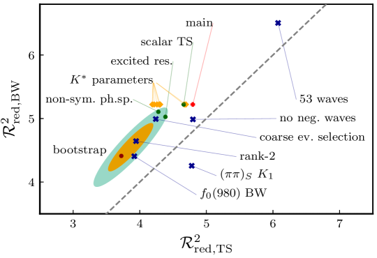
Figure 4 compares the quantity , as defined in Eq. (2) of the main text, for the TS model and the model using a simple Breit-Wigner amplitude for the , for the various studies.
These include using a smaller wave set (“53 waves”), removing negative-reflectivity waves (“no neg. waves”), relaxing the event selection (“coarse ev. sel.”), using rank 2 instead of rank 1 (“rank 2”), and changing the parameterization of the (“”, “”). In an additional study, we use the result of a statistical re-analysis of Adolph et al. (2017) applying the bootstrap technique Efron and Tibshirani (1986) (“bootstrap”).
Also, we consider several variations of the fit model for the TS: (i) a fit with non-Bose-symmetrized phase space (“non-sym. ph. sp.”); (ii) neglecting the spins of the particles involved (similar to Ref. Mikhasenko et al. (2015), “scalar TS”); (iii) including the excitations and in the and waves, respectively (masses and widths fixed to the values from the PDG Tanabashi et al. (2018), “excited res.”);
and (iv) we estimate the effect of further rescattering by varying mass and width of the resonance according to their
uncertainties Tanabashi et al. (2018) (“ parameters”).
We see from Fig. 4 that the TS model systematically yields a slightly smaller than the Breit-Wigner model.
Figure 4:
for the Breit-Wigner model vs. for the TS model.
See main text for details on their definition. The main fit shown in Fig. 2 in the main text, is represented by the red cross, the gray dashed line indicates .
Blue crosses correspond to systematic studies using different data points and green dots
show the fit results with a modified model of the wave.
Fits with a modified lineshape of the resonance are shown by the orange diamonds.
The result of the bootstrap analysis is shown by the filled ellipses
which cover , and, of the obtained sample, respectively;
the fit to the bootstrap-sample mean is represented by the brown point.
III The cross-channel projection integral
The contribution to the dispersion term for the -wave in Eq. (1) that manifests the peaking structure from TS is the -wave. It reads:
(3)
where ,
the phase space factor ,
and is the Källén function, .
To limit the growth of the -wave amplitude, we add a customary Blatt-Weisskopf barrier factor Blatt and Weisskopf (1952); Von Hippel and Quigg (1972) with the size parameter GeV-1.
The projection integral reads:
(4)
where we integrate over the phase space of the system with and . The integration limits as calculated as follows:
(5)
Beyond the physical region, we use analytic continuation with the prescription Bronzan and Kacser (1963).
The function is polynomial in , , and and arises from the product of Wigner d-functions (see Eq. (B12) in Ref. Mikhasenko et al. (2018)),
(6)
with , and .
The term is the denominator of the scattering amplitude, i.e.
(7)
We ensure the correct analytic structure using the Chew-Mandelstam function for the absorptive term Tanabashi et al. (2018); Basdevant and Berger (1977).
Note that .
IV Fit result for all bins
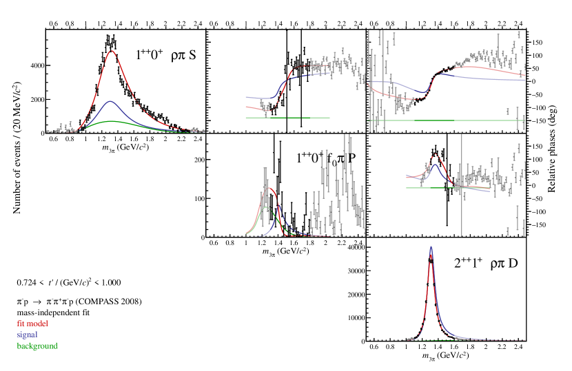
Figures 5 – 15 show the spin-density matrix elements (SDMEs) of the three waves selected for the model fit (data points) and the fit results of the TS model for
all -bins.
The full fit model (red) is decomposed into signal (blue) and background (green) as described in the main text. The intensities are plotted on the diagonal and the complex phase of the interference parts on the off-diagonal. The 3 rows as well as the 3 columns correspond to the , , and -waves.
Figure 5: Spin-density matrix elements of the 3 waves selected for the TS model fit and the corresponding fit results, both shown for the first (lowest) bin of .
The SDMEs as a function of are visualized in the form of a upper-triangular matrix of graphs with the partial-wave intensities on the diagonal and the relative phases between the partial waves on the off-diagonal.
Black crosses correspond to the result of the PWA in bins of and from Ref. Adolph et al. (2017) with statistical uncertainties indicated by vertical lines. The data are overlaid by the TS model curve (red), the contributions from signal (blue) and non-resonant background (green). The fit range is indicated by the color saturation of data points and fit result. Regions
indicated by lower color saturation were not included in the fit; the model curves in these regions are extrapolations.Figure 6: Same as Fig. 5, but for -bin 2.Figure 7: Same as Fig. 5, but for -bin 3.Figure 8: Same as Fig. 5, but for -bin 4.Figure 9: Same as Fig. 5, but for -bin 5.Figure 10: Same as Fig. 5, but for -bin 6.Figure 11: Same as Fig. 5, but for -bin 7.Figure 12: Same as Fig. 5, but for -bin 8.Figure 13: Same as Fig. 5, but for -bin 9.Figure 14: Same as Fig. 5, but for -bin 10.Figure 15: Same as Fig. 5, but for -bin 11.