A Note on Bödewadt-Hartmann Layers

Abstract

This paper addresses the problem of axisymetric rotating flows bounded by a fixed horizontal plate and subject to a permanent, uniform, vertical magnetic field (the so-called Bödewadt-Hartmann problem). The aim is to find out which one of the Coriolis or the Lorentz force dominates the dynamics (and hence the boundary layer thickness) when their ratio, represented by the Elsasser number $A$, varies. After a short review of existing linear solutions of the semi infinite Ekman-Hartmann problem, weakly non-linear analytical solutions as well as fully non-linear numerical solutions are given.

The case of a rotating vortex in a finite depth fluid layer is then studied, first when the flow is steady under a forced rotation and second for spin-down from some initial state. The angular velocity in the first case and decay time in the second are obtained analytically as a function of $A$ using the weakly non linear results of the semi-infinite Bödewadt-Hartmann problem.

Keywords: Hartmann, Ekman-Bödewadt layers, Rotating flows, MHD, Kàrman approximation, axisymetric flows.

1 Introduction

Figure 1: Bödewadt-Hartmann Configuration.

We are concerned here with the interaction of a vortex with a plane surface in the presence of an imposed magnetic field $\mathbf{B}$. The axis of the vortex and the magnetic field are both normal to the surface and, for simplicity, we take the flow to be axisymmetric (see Figure 1). We are interested in characterizing the decay of the vortex, due either to surface friction or to magnetic damping. Such geometries are important in geophysics (motion in planetary interiors are dominated by Coriolis and Lorentz forces), in engineering (for example, in the magnetic damping of turbulence in castings), and in laboratory studies of MHD turbulence.

Our geometry combines two classical problems in fluid mechanics: the Bödewadt layer and the Hartmann layer. These are illustrated in Figure 2. In the Bödewadt problem there is no magnetic field and the fluid is in a state of rigid-body rotation above a plane surface. A boundary layer develops, of approximate thickness,

$$\delta_{\Omega}=\left({\nu/\Omega}\right)^{1\mathord{\left/{\vphantom{12}}\right.\kern-1.2pt}2}$$

where $\nu$ is the fluid viscosity and $\Omega$ is the core rotation rate. Within this boundary layer there is an imbalance between the local centrifugal force, $\rho u_{\theta}^{2}/r$, and the radial pressure gradient, ${\partial p}\mathord{\left/{\vphantom{{\partial p}{\partial r}}}\right.\kern-1.2pt}{\partial r}$, which is established outside the boundary layer by the rigid-body rotation . That is, the core rotation sets up a radial pressure gradient of ${\partial p}\mathord{\left/{\vphantom{{\partial p}{\partial r}}}\right.\kern-1.2pt}{\partial r}=\rho\Omega^{2}r$ and this is imposed on the boundary layer where $u_{\theta}$ is locally diminished due to viscous drag. The result is a radial inflow within the boundary layer. By continuity there is an upward flux of mass out of the Bödewadt layer and into the core, and in the configuration shown in Figure 2(a) this leads to a weak secondary flow in the core, u_p. This secondary (poloidal) flow is crucial to the development of the vortex, since it sets up a Coriolis force, $-2u_{r}\Omega{\rm{\bf\hat{e}}}_{\theta}$, which opposes the core motion and tends to decelerate the vortex. This kind of motion is seen, for example, in the spin-down of a stirred cup of tea.

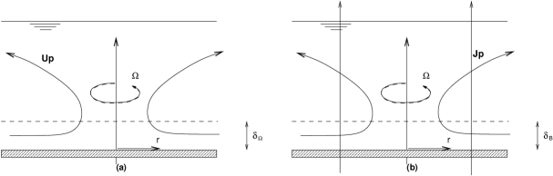
Figure 2: Classical Boundary layers. (a) Bödewadt layer; (b) Hartmann layer. In the Hartmann layer, B is dominant in the sense that $\sigma B^{2}>>\rho\Omega$.

The Hartmann problem is shown in Figure 2(b). Here the inertial forces are weak and the Lorentz force is strong in the sense that the Elsasser number

$$A=\frac{\sigma B^{2}}{2\rho\Omega}$$ (1)

is assumed large. ($\sigma$ is the electrical conductivity of the fluid.) A boundary layer is again established, although this time it turns out to have a thickness of the order of

$$\delta_{B}=\left({\nu\tau}\right)^{1\mathord{\left/{\vphantom{12}}\right.\kern-1.2pt}2}\;\;\;\;,\;\;\;\;\;\tau^{-1}=\sigma B^{2}/\rho$$ (2)

where $\tau$ is the so-called Joule damping time. Within this boundary layer an electric current flows in accordance with Ohm’s law

$${\rm{\bf J}}=\sigma\left({{\rm{\bf u}}\times{\rm{\bf B}}-\nabla V}\right)$$ (3)

where $V$ is the electrostatic potential. (The induced magnetic field, defined via $\nabla\times{\rm{\bf b}}=\mu{\rm{\bf J}}$, is neglected throughout on the assumption that $\mu\sigma u\delta$ is small. This is valid in laboratory and engineering applications, but is not always true in the core of the earth.) The electric field, ${\rm{\bf E}}=-\nabla V$, in the Hartmann layer is set by the electric field in the core flow, ${\rm{\bf E}}=-\Omega rB{\rm{\bf\hat{e}}}_{r}$, and this dominates the weaker ${\rm{\bf u}}\times{\rm{\bf B}}$ term in the boundary layer. The net result is radially inward flow of current. Continuity of current then requires that there is an upward flow of current out of the boundary layer and into the core. In the configuration shown in Figure 2(b) this leads to a weak poloidal current, $\mathbf{J}_{p}$, in the core. (Note the similarity between u_p and J_p in Figures 2(a) and 2(b).) This core current is crucial since it results in a Lorentz force ${\rm{\bf J}}\times{\rm{\bf B}}=-J_{r}B{\rm{\bf\hat{e}}}_{\theta}$ which retards the core vortex.

The crucial feature of both the Bödewadt and Hartmann flows is that they constitute active boundary layers, in the sense that they react back on the core flow which created them in the first place. The problem of interest here is shown in Figure 3. The Elsasser number is allowed to be big or small, so that we may capture both the Bödewadt problem, when $A\to 0$, and the Hartmann problem, $A$ $\to$ $\infty$. When $A\sim 1$ we expect both phenomena to be present. The questions which are important are: (i) how does the boundary layer thickness scale with $A$; and (ii) for a given value of $A$, is the deceleration of the core vortex due primarily to the Coriolis force, $-2u_{r}\Omega{\rm{\bf\hat{e}}}_{\theta}$, or to the Lorentz force, $-J_{r}B{\rm{\bf\hat{e}}}_{\theta}$?

There is close correspondence between our problem and the well-known Ekman-Hartmann layer. This latter is shown in Figure 4. An Ekman layer is formed when there is an infinitesimal difference in rotation between a rapidly rotating fluid and an adjacent, plane surface. When the surface rotates slightly slower than the fluid we find a secondary flow very like that in the Bödewadt problem. Indeed, the mechanism which generates the poloidal flow is essentially the same as in a Bödewadt layer. Thus, phenomenologically, Ekman layers and Bödewadt layers are very similar. When a magnetic field is added to an Ekman layer we get the Ekman-Hartmann problem, which shares many of the same characteristics as a Bödewadt-Hartmann layer. However, one of the main differences is that, when viewed in a rotating frame of reference, inertia is negligible in the Ekman-Hartmann problem. (In fact, we interpret the phrase ‘rapid rotation’ to mean that ${\rm{\bf u}}\cdot\nabla{\rm{\bf u}}$ is negligible by comparison with the Coriolis force, $2{\rm{\bf u}}\times\Omega$.) Thus the Ekman and Ekman-Hartmann problems are linear. The Bödewadt-Hartmann problem, on the other hand, is not.

The layout of the paper is as follows. In section 2 we review the properties of an Ekman-Hartmann layer in a semi-infinite fluid. The local properties of such layers are well-known. (See, for example, [1].) However, we are interested here in axisymmetric flows of the Karman type ($u_{r}$ and $u_{\theta}$ linear in $r)$ and so we redevelop the conventional analysis in cylindrical polar coordinates and restrict solutions to those with Karman similarity. This allows us to place the subsequent non-linear problem in context. Next, in section 3, we focus on Bödewadt-Hartmann layers. Once again, the discussion is restricted to a semi-infinite domain. Here we develop the ideas of [2] and [3], who noted that such layers admit self-similar solutions of the Karman type. However, we go further than these authors, developing approximate solutions for these Karman-like flows, the validity of which is confirmed by fully non-linear numerical simulations.

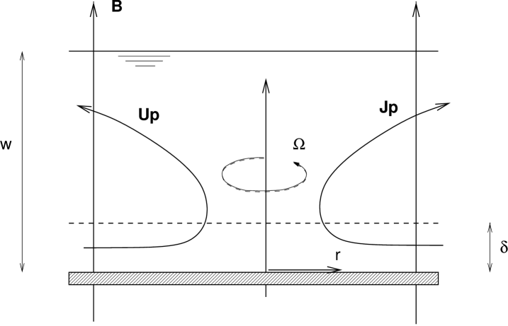
Figure 3: Bödewadt-Hartman geometry. The secondary flow generates a Coriolis Force, $2u_{r}$$\Omega$, which tends to oppose the vortex outside the boundary layer. The induced current interacts with B to create a Lorentz force $J_{r}B,$which also opposes the vortex.

The novel results of the paper lie in sections 4 and 5 where we move from semi-infinite domains to confined flows. There is then a coupling of the core motion to the boundary layer through the radial components of u and J (see Figure 3). The associated Lorentz and Coriolis forces tend to oppose the core motion and the central questions now relate to the influence of the boundary layer on the external vortex, rather than on the boundary layer itself. There are two canonical problems of interest here. One is the steady-state case in which the core vortex is maintained by some external azimuthal force (say that generated by a rotating magnetic field) and the other is the transient problem of spin-down from some initial state of rotation. In both cases we are interested in determining the dominant force balance in the core. (Does the primary resistance to motion come from the Lorentz force or the Coriolis force?) In the steady flow we determine the magnitude of $\Omega$ as a function of $A$, while in the transient problem we calculate the spin-down time, which also depends on $A$.

There are two dimensionless groups which appear throughout. We have already mentioned the Elsasser number which provides a measure of the relative sizes of the Lorentz and Coriolis forces,

$$A=\frac{\sigma B^{2}}{2\Omega\rho}=\frac{1}{2\Omega\tau}=\frac{\delta_{\Omega}^{2}}{2\delta_{B}^{2}}.$$ (4)

This usually lies in the range $0<A<10$, and very rarely exceeds 50. On the other hand, the Reynolds number, $Re=\Omega W^{2}/\nu$ is invariably very large (Here $W$ is the depth of fluid: see Figure 3). Thus we consider the range of parameters:

$$0<A<<Re\;\;\;\;,\;\;\;\;\;Re>>1.$$ (5)

However, the flow is assumed to be laminar so that, in practice, $Re$ cannot be made too large.

2 Ekman-Hartmann Layers of the Karman Type

Ekman and Hartmann layers are usually described as a local phenomenon, the boundary layer being the result of some local difference in the core and boundary velocities. As a result, they are usually discussed in a planar framework, using cartesian coordinates. Since we are ultimately interested in axisymmetric, nonlinear flows of the Karman type, we shall take a different approach. We restrict ourselves to axisymmetric motion, described using cylindrical polar coordinates ($r$,$\theta$,$z)$, and look for Ekman-Hartmann layers which possess Karman similarity ($u_{r}$ and $u_{\theta}$ linear in $r$).

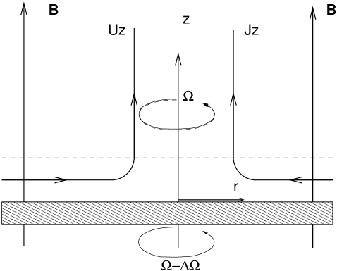
Figure 4: Ekman-Hartmann geometry

Consider a conducting fluid which fills the domain $z>0$ and rotates above a plane, insulating surface located at $z=0$ (see Figure 4). Far from the surface we have rigid-body rotation, $u_{\theta}=\Omega r$, and the surface itself rotates at the lower rate,$\Omega-\Delta\Omega$, $\Delta\Omega<<\Omega$. Both $\Omega$ and $\Delta\Omega$ are assumed to be constant and so, in a frame of reference rotating with the unperturbed fluid we have,

$$0 = 2{\rm{\bf u}}\times\Omega-\nabla\left({p/\rho}\right)+\nu\nabla^{2}{\rm{\bf u}}+{\rm{\bf J}}\times{\rm{\bf B}}/\rho$$ (6)

$${\rm{\bf J}} = \sigma\left({{\rm{\bf u}}\times{\rm{\bf B}}-\nabla V}\right),$$ (7)

where B is a uniform, imposed magnetic field which is parallel to $\Omega$. (The inertial term, ${\rm{\bf u}}\cdot\nabla{\rm{\bf u}}$, is assumed to be much smaller than the Coriolis force, and so is omitted from (6).) Taking the curl of (6) twice and substituting for J yields,

$$\nu\nabla^{4}{\rm{\bf u}}-\left({\sigma/\rho}\right)\left({{\rm{\bf B}}\cdot\nabla}\right)^{2}{\rm{\bf u}}=2\left({\Omega\cdot\nabla}\right)\mathbf{\omega},$$ (8)

where $\mathbf{\omega}=\nabla\times{\rm{\bf u}}$. From this we may obtain the governing equation for u:

$$\left[{\nu\nabla^{4}-\frac{1}{\tau}\,\frac{\partial^{2}}{\partial z^{2}}}\right]^{2}{\rm{\bf u}}+\left({2\Omega\cdot\nabla}\right)^{2}\nabla^{2}{\rm{\bf u}}=0$$ (9)

(See, for example, [1]). Let us now look for axisymmetric solutions of the Karman form:

$${\rm{\bf u}}={\rm{\bf u}}_{p}+{\rm{\bf u}}_{\theta}=-\nabla\times\left[{r\Psi(z){\rm{\bf\hat{e}}}_{\theta}}\right]+rG(z){\rm{\bf\hat{e}}}_{\theta}.$$ (10)

We find that both $G$ and ${\Psi}^{\prime}(z)$ satisfy,

$$\left[{\frac{\delta_{\Omega}^{2}}{2}\,\frac{\partial^{2}}{\partial z^{2}}-A}\right]^{2}\left({G,{\Psi}^{\prime}}\right)+\left({G,{\Psi}^{\prime}}\right)=0,$$ (11)

where $\delta_{\Omega}$ is the Bödewadt (or Ekman) boundary-layer scale,

$$\delta_{\Omega}=\left({\nu/\Omega}\right)^{1\mathord{\left/{\vphantom{12}}\right.\kern-1.2pt}2}.$$ (12)

Next we solve for $G$ and ${\Psi}^{\prime}$. After a little algebra we find,

$$\frac{u_{r}}{\Delta\Omega r} = -\exp\left[{-Rz/\delta_{\Omega}}\right]\sin\left[{z/R\delta_{\Omega}}\right]$$ (13)

$$\frac{u_{\theta}}{\Delta\Omega r} = -\exp\left[{-Rz/\delta_{\Omega}}\right]\cos\left[{z/R\delta_{\Omega}}\right]$$ (14)

$$\frac{u_{z}-\left({u_{z}}\right)_{\infty}}{2\Delta\Omega\delta_{\Omega}} = -\exp\left[{-Rz/\delta_{\Omega}}\right]\,\,\left[{\frac{R}{1+R^{4}}\cos\left({\frac{z}{R\delta_{\Omega}}}\right)+\frac{R^{3}}{1+R^{4}}\sin\left({\frac{z}{R\delta_{\Omega}}}\right)}\right]$$ (15)

$$\left({u_{z}}\right)_{\infty} = 2\Delta\Omega\delta_{\Omega}\frac{R}{1+R^{4}}$$ (16)

where $R$ is a function of the Elsasser number,

$$R=\left[{A+\left({1+A^{2}}\right)^{1\mathord{\left/{\vphantom{12}}\right.\kern-1.2pt}2}}\right]^{1\mathord{\left/{\vphantom{12}}\right.\kern-1.2pt}2}$$ (17)

Returning now to (7) we evaluate J. In particular we find that, outside the boundary layer, we have,

$$\left({J_{z}}\right)_{\infty}=2\sigma B\Delta\Omega\delta_{\Omega}\frac{R^{3}}{1+R^{4}}$$ (18)

It is convenient that all of the electromagnetic effects are bound up in the single parameter, $R$. If we let $A$ $\to$ 0 we capture the conventional Ekman solution,

$$\frac{u_{r}}{\Delta\Omega r}=-\exp\left[{-z/\delta_{\Omega}}\right]\sin\left[{z/\delta_{\Omega}}\right]\quad \quad\frac{u_{\theta}}{\Delta\Omega r}=-\exp\left[{-z/\delta_{\Omega}}\right]\cos\left[{z/\delta_{\Omega}}\right]$$ , (19)

$$\left({u_{z}}\right)_{\infty} = \Delta\Omega\delta_{\Omega}$$ (20)

Conversely, if we let $A\to\infty$ then we obtain the Hartmann solution,

$$u_{r}=u_{z}=0,\quad u_{\theta}=-\Delta\Omega r\,\exp\left[{-z/\delta_{B}}\right],\quad(J_{z})_{\infty}=2\sigma B\Delta\Omega\delta_{B}$$ (21)

Thus we have a smooth transition from a Coriolis dominated flow to a Lorentz dominated motion. Of particular interest is the far-field values of u and J, since it is these which feed into the core flow. In dimensionless form these are related by,

$$\frac{\left({J_{z}}\right)_{\infty}}{\sigma B(u_{z})_{\infty}}\,=A+\left({1+A^{2}}\right)^{1\mathord{\left/{\vphantom{12}}\right.\kern-1.2pt}2}$$ (22)

If we define the boundary-layer thickness, $\delta$, to be distance over which $u$ declines by a factor of $e^{-1}$, then we also have,

$$\delta^{2}=\frac{\delta_{\Omega}^{2}}{\left({1+A^{2}}\right)^{1/2}+A}=\frac{2\delta_{B}^{2}}{1+\left({1+A^{-2}}\right)^{1/2}}$$ (23)

Note that when $\delta_{\Omega}$ and $\delta_{B}$ are very different there is still only one relevant length scale, $\delta$. That is, there is no nesting of the boundary layers, with one lying within the other. Comparing (22) with (23) we see that, for arbitrary $B$,

$$\frac{(J_{z})_{\infty}}{\sigma B(u_{z})_{\infty}}=\left({\frac{\Omega\delta^{2}}{\nu}}\right)^{-1}$$ (24)

The inward flow of mass and current in the boundary layer is essentially for the reasons given in Section 1. The mass flow arises from the radial pressure gradient set up in the core flow. A similar argument explains the radial current. Outside the boundary layer the electrostatic term in Ohm’s law (7) is balanced by $\mathbf{u_{\theta}}\times{\rm{\bf B}}$

$$E_{r}=-\frac{\partial V}{\partial r}=-u_{\theta}B=-\Omega Br$$

This electric field is also imposed on the boundary layer where $-u_{\theta}B$ is insufficient to balance it. The result is a flow of current as shown in Figure 4.

3 Bödewadt-Hartmann Layers in a Semi-infinite Fluid

3.1 The Governing Equations

Let us now turn to the non-linear problem in which the plate in Figure 4 is stationary. That is, we consider a Bödewadt-Hartmann layer in a semi-infinite fluid. As noted by [2], such a layer admits a Karman-like solution in which $u_{\theta}$ and $u_{r}$ are linear in $r$. This time our governing equations, in an absolute frame of reference, are

$${\rm{\bf u}}\cdot\nabla{\rm{\bf u}}=-\nabla\left({p/\rho}\right)+\nu\nabla^{2}{\rm{\bf u}}+{\rm{\bf J}}\times{\rm{\bf B}}/\rho$$ (25)

$${\rm{\bf J}}=\sigma\left({{\rm{\bf u}}\times{\rm{\bf B}}-\nabla V}\right)$$ (26)

From this we find

$$\nu\nabla^{4}{\rm{\bf u}}-\left({\sigma/\rho}\right)\left({{\rm{\bf B}}\cdot\nabla}\right)^{2}{\rm{\bf u}}=\nabla\times\nabla\times({\rm{\bf u}}\times\bf{\omega})$$ (27)

which might be compared with (8). We now look for Karman-like solutions of the form:

$${\rm{\bf u}}=\left[{\Omega rF(z/l),\;\;\Omega rG(z/l),\,\;\;\Omega lH(z/l)}\right]\;,\;p=\frac{1}{2}\rho\Omega^{2}\left[{r^{2}+\hat{P}(z/l)}\right]$$

where $l$ is some (as yet) unspecified length scale. The boundary conditions on $F$, $G$, $H$ and $\hat{P}$ are:

$${\begin{array}[]{*{20}c}{z=0\;\;:\,\;\;\;F=0\;\;\;,\;\;\;G=0\;\;,\;\;\;H=0\hfill}\\ {z\to\infty\;\;:\,\;\;\;F=0\;\;\;,\;\;\;G=1\;\;,\;\;\;\hat{P}=0.\hfill}\\ \end{array}}$$

Substitution of the expression for u into (27) yields three ordinary differential equations for $F$, $G$, $H$ and $\hat{P}$. However, from a physical point of view it is more interesting to work with (25). First we note that the axial component of (25) gives a differential equation for $\hat{P}$, from which we may deduce that $\hat{P}\sim\delta^{2}$. In other words, $\hat{P}$ is a small perturbation in pressure within the boundary layer. Next we turn to the radial and azimuthal components of (25). This, in turn, requires that we evaluate J $\times$ B. From Ohm’s law it is readily confirmed that

$${\rm{\bf J}}\times{\rm{\bf B}}=\left[{-\sigma u_{r}B^{2},\;\;-\sigma B(u_{\theta}B-\partial V/\partial r),\,0}\right]$$ (28)

In order to fix $V$ we specify that there is no radial current, and hence no azimuthal Lorentz force, outside the boundary layer. In addition, (26) demands

$$\nabla^{2}V=\nabla\cdot\left({{\rm{\bf u}}\times{\rm{\bf B}}}\right)={\rm{\bf B}}\cdot\mathbf{\omega}$$

from which we deduce that the electrostatic potential is of the form,

$$V=\frac{1}{2}B\Omega r^{2}-2B\Omega\int{\int{(1-G)dzdz}}$$ (29)

It follows that the Lorentz force is simply,

$${\rm{\bf J}}\times{\rm{\bf B}}=\left[{-\sigma B^{2}u_{r},\;-\sigma B^{2}(u_{\theta}-\Omega r),\;0}\right]$$ (30)

The radial and azimuthal components of (25), along with the continuity equation, then yield

$$F^{2}+H{F}^{\prime}-G^{2}+1=(\nu/\Omega l^{2}){F}^{\prime\prime}-2AF$$ (31)

$$2FG+{G}^{\prime}H=(\nu/\Omega l^{2}){G}^{\prime\prime}-2A[G-1]$$ (32)

$${H}^{\prime}+2F=0.$$

Finally, it is of interest to determine the magnitude of the current leaving the boundary layer. This is fixed by (26) in the form,

$$\nabla\times{\rm{\bf J}}=\sigma({\rm{\bf B}}\cdot\nabla){\rm{\bf u}}$$ (33)

the axial component of which yields

$$(J_{z})_{\infty}=2\sigma B\Omega\int_{0}^{\infty}{(1-G)dz}$$ (34)

It is convenient to choose $l=\delta_{\Omega}$, the Bödewadt boundary layer thickness. Our governing equations for u then simplify to

$${F}^{\prime\prime}=F^{2}+H{F}^{\prime}+(1+G)(1-G)+2AF$$ (35)

$${G}^{\prime\prime}=2FG+H{G}^{\prime}+2A(G-1)$$ (36)

$${H}^{\prime}=-2F,$$ (37)

These equations are readily solved numerically to give F, G and H. This then yields $(J_{z})_{\infty}/\sigma B\Omega\delta_{\Omega}$ and $(u_{z})_{\infty}/\Omega\delta_{\Omega}$ as functions of A, which is the primary information we need for the problems of sections 4 and 5. However, we shall see that it is possible to obtain analytical estimates of $J_{z}$ and $u_{z}$, which turn out to be more useful.

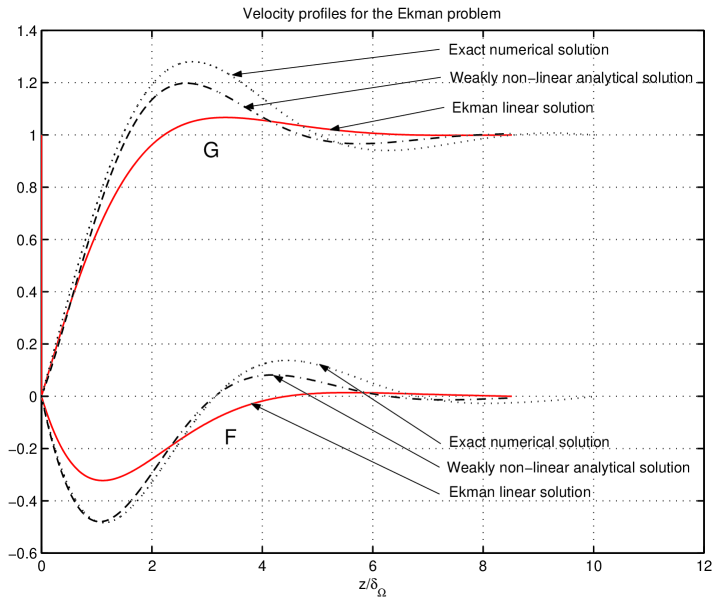
Figure 5: Bödewadt layer profiles obtained under different assumptions. Solid: analytical solution of the Ekman problem. Dotted: numerical solution for the Bödewadt problem calculated in section 4. Dashed: weakly non-linear solution. Curves above the $z-$ axis represent azimuthal velocity profiles and curves below represent radial velocity profiles.

When $A=0$ (no magnetic field) our governing equations represent the standard equations describing a Bödewadt layer. Let us consider this special case for a moment. The governing equations are,

$${F}^{\prime\prime}=(1+G)(1-G)+F^{2}+H{F}^{\prime}$$ (38)

$${G}^{\prime\prime}=2FG+{G}^{\prime}H$$ (39)

$${H}^{\prime}=-2F$$ (40)

On integration these yield $F_{\infty}=0$, $G_{\infty}=1$ and $H_{\infty}=1.349$. Actually, as Greenspan points out, a rough approximation to the Bödewadt solution may be obtained by replacing the non-linear inertial terms on the right of (38) and (39) by the Coriolis force, $-2{\rm{\bf u}}_{r}\times\Omega$, where u_r is the velocity measured in a frame of reference rotating with the fluid at infinity. This gives

$${F}^{\prime\prime}=2(1-G)\;\;\;,\;\;\;\;{G}^{\prime\prime}=2F$$ (41)

Of course, this leads to the Ekman solutions (19), with $\Delta\Omega$ set equal to $\Omega$. Such a procedure is usually called the linear, or Ekman, approximation. Surprisingly, there is a reasonable qualitative agreement between the linear (Ekman) approximation and the exact non-linear solution (see [4], and Figure 5). In both cases the solution takes the form of a decaying oscillation of $F$ and $G-1$, and the frequency of oscillation is very similar in the two cases. However, the linear approximation over-estimates the exponential-like decay of $F$ and $G-1$ by a factor of about 2. It also underestimates $H_{\infty}$ by around 35%.

Turning now to the other extreme, of large $A$, equation (36) reduces to

$${G}^{\prime\prime}=2A(G-1)$$ (42)

This, plus (34), yields

$$(J_{z})_{\infty}=2\sigma B\Omega\delta_{B}$$ (43)

$$G=1-\exp\left[{-z/\delta_{B}}\right]$$ (44)

Of course, these coincide exactly with the results of the linear Ekman-Hartmann analysis (in the limit of large $A)$. The exact correspondence between (44) and (21), when $\Delta\Omega$ is set equal to $\Omega$, is inevitable since in both cases the non-linear inertial terms are neglected.

The general picture, then, is that the linear Ekman-Hartmann approximation (with $\Delta\Omega$ set equal to $\Omega)$ yields results which are qualitatively similar to the Bödewadt-Hartmann problem when $A$ = 0, and that the two analyses coincide when $A$ becomes large. We now show how to obtain an improved approximation to the Bödewadt-Hartmann solution which has a simple algebraic form. We follow a method originally developped for Bödewadt layers (see for example [6]).

3.2 An Approximate Analytical Solution

Before tackling the weakly non-linear problem, it is important to note that the full system (35)-(36) with associated boundary conditions need not have a unique solution (see [5]). Physically, however this most likely relates to the absence of lateral boundary conditions, which appear to play a determining role in real experiments. The solution we look at is the physically most important, in that it is the one which appears in practice when fixed lateral boundaries are included at large radius.

Let us return to (35) and (36) and look for solutions at large $z$. If we linearise the equations around the far-field solution $(F,G,H)=(0,1,H_{\infty})$ we obtain

$${F}^{\prime\prime}-H_{\infty}{F}^{\prime}-2AF=-2\hat{G}$$ (45)

$${\hat{G}}^{\prime\prime}-H_{\infty}{\hat{G}}^{\prime}-2A\hat{G}=2F$$ (46)

where $\hat{G}=G-1$. This yields oscillatory solutions of the form,

$$\hat{G}_{\infty},F_{\infty}\sim\exp\left[{-(\hat{R}-H_{\infty}/2)z/\delta_{\Omega}}\right]\exp\left[{\pm jz/\hat{R}\delta_{\Omega}}\right]$$ (47)

where

$$\hat{R}=\left[{\hat{A}+(1+\hat{A}^{2})^{1/2}}\right]^{1/2},\quad\hat{A}=A+H_{\infty}^{2}/8,\quad j^{2}=-1$$ (48)

Note that if we set $H_{\infty}$ to zero in (47) and (48) we obtain the linear Ekman estimate. Let us now make two approximations. First, we take $H_{\infty}$ to be given by the linear Ekman-Hartmann solution (17):

$$H_{\infty}=\frac{2R}{1+R^{4}}\;\;\;\;,\;\;\;\;\;R=\left[{A+\left({1+A^{2}}\right)^{1\mathord{\left/{\vphantom{12}}\right.\kern-1.2pt}2}}\right]^{1\mathord{\left/{\vphantom{12}}\right.\kern-1.2pt}2}$$ (49)

Second, we assume that our estimate of $\hat{G}_{\infty}$ and $F_{\infty}$ are valid, not just for large $z$, but for all $z$. If this is true then,

$$\hat{G}=G-1=-\exp\left[{-(\hat{R}-H_{\infty}/2)z/\delta_{\Omega}}\right]\cos(z/\hat{R}\delta_{\Omega})$$ (50)

$$F=-\exp\left[{-(\hat{R}-H_{\infty}/2)z/\delta_{\Omega}}\right]\sin(z/\hat{R}\delta_{\Omega})$$ (51)

Let us now see how our guesses have faired. We look first at small $A$. When $A$ = 0 (a pure Bödewadt layer) we have $\hat{R}=1.064$ and the resulting curves for $F$ and $G$ are plotted in Figure 5. The exact solution and the linear Ekman approximation are also given for comparison. Evidently, there is a reasonable correspondence between (50) and (51) and the exact solution. For large $A$, on the other hand, (50) and (51) reduce to

$$F=0\,\,\,,\,\,\,G=1-\exp\left[{-z/\delta_{B}}\right]$$ (52)

which corresponds precisely with both the exact solution and the Ekman approximation.

Given that (50) and (51) are reasonably accurate for small $A$, and exact for large $A$, our proposal is to adopt them as approximations to the Bödewadt-Hartmann layer in sections 4 and 5. The corresponding current distribution is given by (34) and this, combined with (50), fixes $J_{z}$. In summary then, we have the following estimates of $(u_{z})_{\infty}$ and $(J_{z})_{\infty}$:

$$\frac{(u_{z})_{\infty}}{\Omega\delta_{\Omega}}=\frac{2R}{1+R^{4}}\;\;\;\;,\;\;\;\;R=\left[{A+(1+A^{2})^{1\mathord{\left/{\vphantom{12}}\right.\kern-1.2pt}2}}\right]^{{\,\;1}\mathord{\left/{\vphantom{{\,\;1}2}}\right.\kern-1.2pt}2}$$ (53)

$$\frac{(J_{z})_{\infty}}{2\sigma B\Omega\delta_{\Omega}}=\frac{\hat{R}^{2}(\hat{R}-H_{\infty}/2)}{1+\hat{R}^{2}(\hat{R}-H_{\infty}/2)^{2}}\;\;\;\;,\;\;\;\;\hat{R}=\left[{\hat{A}+(1+\hat{A}^{2})^{1\mathord{\left/{\vphantom{12}}\right.\kern-1.2pt}2}}\right]^{\;1\mathord{\left/{\vphantom{12}}\right.\kern-1.2pt}2}$$ (54)

3.3 Numerical Solutions of the Governing Equations

Before adopting (53) and (54) it seems sensible to compare these with the exact solutions of (35)-(37) obtained by numerical means. First of all, the problem is expressed on a finite interval, using the variable shift $\frac{z}{\delta_{\Omega}}=-\ln\left({1-t}\right)$. The resulting system is then discretized with a centred finite differences method. The associated non-linear set of equations is solved using a Newton-Raphson algorithm (the equivalent first-order system is then 5-dimensional). In order to be able to compute the large number of points required to reach high values of $z$ in a reasonable computation time, we need a fast matrix inversion. We proceed as follows: the $5n$ equations (where $n$ is the number of points in the mesh) are ordered so that the finite difference system is represented by a bi-diagonal 5$\times$5-block matrix (diagonal blocks $J_{k}$ and sub-diagonal blocks $K_{k}$ ) with a block C in the upper right corner containing the boundary conditions:

$$\left[{{\begin{array}[]{*{20}c}{J_{1}\hfill}&\hfill\hfil&\hfill\hfil&C\hfill\\ {K_{2}\hfill}&{J_{2}\hfill}&\hfill\hfil&\hfill\hfil\\ \hfill\hfil&{...\hfill}&{...\hfill}&\hfill\hfil\\ \hfill\hfil&\hfill\hfil&{K_{n}\hfill}&{J_{n}\hfill}\\ \end{array}}}\right]\times\left[{{\begin{array}[]{*{20}c}{X_{1}\hfill}\\ {X_{2}\hfill}\\ {...\hfill}\\ {X_{n}\hfill}\\ \end{array}}}\right]=\left[{{\begin{array}[]{*{20}c}{F_{1}\hfill}\\ {F_{2}\hfill}\\ {...\hfill}\\ {F_{n}\hfill}\\ \end{array}}}\right]$$ (55)

A first system S₁ is formed with the first block-line. It involves unknown blocks $X_{1}$and $X_{n}$ (the unknown vector $X$ is split into $n$ 5-dimensional “block-vectors”). The unknown $X_{n}$ is expressed recursively as a function of $J_{k}$, $K_{k}$ / k$\in${2..n} and $X_{1}$ thanks to the bi-diagonal structure of the matrix. The resulting system of 5 equations ($i.e.$ one block) can then be added to S₁ to give an invertible system whose solutions are $X_{1}$ and $X_{n}$. The other unknowns are then deduced recursively. This inversion method requires a number of operations proportional to $n$ (versus $n^{2}$, if the Jacobian matrix had been directly inverted) which considerably reduces the computation time. The accuracy of the procedure was checked by comparing the analytical and numerical solutions of the Ekman problem.
We first investigate the non-magnetic case ($A=0$). Figure 5 shows a comparison between different estimates the Bödewadt problem: the fully non-linear solution of (38)-(40) (obtained numerically on 23000 points), the weakly non-linear solution (50)-(51) and the linear Ekman approximation. It appears that non-linear effects are responsible for rather stronger oscillations in the velocity profiles than those predicted by (50)-(51). This is consistent with the assumptions on which the analytical solution (50)-(51) relies, as the latter extrapolates a solution (47)-(48) valid for large $z$ and takes the value returned by the linear Ekman-Hartmann theory for $H_{\infty}$. The associated Ekman pumping is then underestimated by 35% (compared to the fully non-linear solution), and so are the radial velocity and the oscillations. For $A=0$, the discrepancy between (50)-(51) and the full numerical result is below 10% on azimuthal and radial velocity, which is not such an expensive price to pay for an analytical solution.

Figure 6: Velocity profiles in the Bödewadt-Hartmann layer for values of $A$ in the range $10^{-3}\to 10^{3}$. The arrows go from low to high $A$ curves.

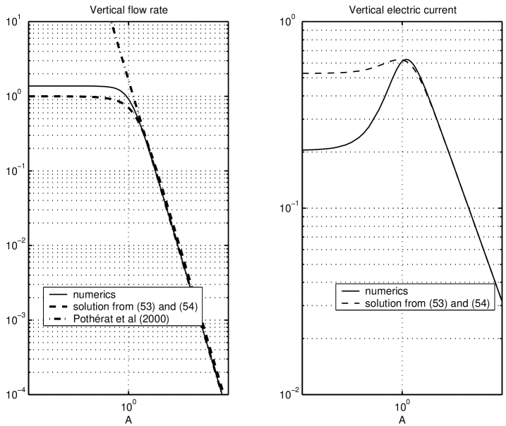
Figure 7: Vertical velocity (left) and vertical electric current (right) at the edge of the Bödewadt-Hartmann layer. The numerical simulation is given by the solid line and the approximate solution (53-54) by the dashed line.

We now turn our attention toward the non-linear MHD case (A$\neq$0). System (38-40) is solved numerically for values of $A$ taken in the range $10^{-3}\rightarrow 10^{3}$ (figure 7). For A$<1$, the velocity profiles across the layer are close to the well-known Bödewadt layer profile, but with the difference that the oscillating part of the profile is softened by the action of the magnetic field, as predicted by (50)-(51). For $A>>1,$ the profile is rather close to the exponential profile of the Hartmann layer without oscillations. In this case, the results of the numerical simulation may be compared not only with our approximate solution (50)-(51), but also with those of [7], which applies to Hartmann layers with weak inertia. Figure 7 shows the various estimates of $(u_{z})_{\infty}$ and $(J_{z})_{\infty}$, the vertical velocity and current leaving the boundary layer. The left-hand figure shows $(u_{z})_{\infty}$. It can be seen that our approximate solution (53) is close to the exact value for all $A$. The model of [7] is accurate for $A>2$ but not for small $A$. The right-hand figure shows $(J_{z})_{\infty}$ corresponding to approximation (54), as well as the exact, computed value. The approximate solution is good for $A>1$ but overestimates the current for $A<1$.
Note that [8], [9] have investigated the stability of geophysical Ekman-Hartmann layers. Their study differs from the present problem by the geometry (spherical) and also by the fact that magnetic field and rotation are not aligned nor orthogonal to the layer. The results however do not depend on the co-latitude (along which the angle between the layer and the rotation vary) which suggest that they might be of some relevance here. In the non-magnetic case, it is found that the flow is non-linearly unstable for values of the Reynolds number scaled on the boundary layer thickness above 0.55 ($A=0)$ and linearly unstable for values above 40. The presence of the magnetic field makes the flow more stable so that these values are changed to 0.71 and 160 respectively for $A=1$. (The linear stability value corresponds to the co-latitude for which the rotation is orthogonal to the boundary layer). This is consistent with the fact that plane Hartmann layers are indeed much more stable than rotation layers. (They have a linear stability threshold around 50000, according to [10]). These results underline the fact that the solutions obtained numerically in this section are only valid below a threshold value of $\Omega$, which increases with $A$. For stronger rotation, [9] showed that traveling waves appear in the plane of the layer.

4 Forced Vortex in a Confined Layer

We now look at flows which are typical of laboratory experiments. In particular, we consider a pool of depth $W$, the depth being assumed to be much greater than the Bödewadt-Hartmann boundary layer thickness (figure 3). That is, we restrict ourselves to free surface flows which have a high Reynolds number. There are two particular cases of interest. The first is where a steady vortex is maintained by an external azimuthal force, say that produced by a rotating magnetic field. We shall study that problem here. The second, which we leave to section 5, is the transient problem of spin down from some initial state of rotation. The geometry for both cases is shown in Figure 3. For simplicity, we model the free surface at $z=W$ as a symmetry plane.

In this section we look at the case where the vortex is maintained by the body force,

$${\rm{\bf F}}=\frac{1}{2}\Omega_{f}r{\rm{\bf\hat{e}}}_{\theta}\;\;\;\;\;\;\;\;\;\;,\;\;\Omega_{f}=constant$$ (56)

Since $F_{\theta}$ is linear in $r$ we can once again look for solutions of the Karman type. The resulting equations are of a form similar to (28)-(34). That is, if we look for solutions of the form

$${\rm{\bf u}}=\left[{\Omega_{c}rF\left({z/l}\right)\;\;,\;\;\;\Omega_{c}rG(z/l)\;\;,\;\;\;\Omega_{c}lH(z/l)}\right]$$ (57)

we find,

$${H}^{\prime}+2F=0$$ (58)

$$F^{2}+H{F}^{\prime}-G^{2}+1=(\nu/\Omega_{c}l^{2}){F}^{\prime\prime}-2AF$$ (59)

$$2FG+{G}^{\prime}H=(\nu/\Omega_{c}l^{2}){G}^{\prime\prime}+\frac{1}{2}\left({\Omega_{f}/\Omega_{c}}\right)^{2}-2A\left[{G-f}\right]$$ (60)

Here $\Omega_{c}$ is a typical rotation rate outside the boundary layer, $l$ is an arbitrary length scale, and $f$ is related to the radial gradient of $V$,

$$f=\left({\Omega_{c}rB}\right)^{-1}\frac{\partial V}{\partial r}$$

(See equation (28) for the origin of the term $G-f$.) The only differences between (58)-(60) and (31)-(32) is that: (i) we have incorporated the driving force $\frac{1}{2}\Omega_{f}^{2}r$ ; and (ii) we have yet to specify $f$. In the semi-infinite domain problem of section 3 we specified that $J_{r}$ is zero outside the boundary layer and this fixed $f$ as $f=1$. However, it is clear from Figure 3 that this is no longer legitimate. Now we know that there is a uniform flux of current out of the boundary layer, which we called $(J_{z})_{\infty}$. Thus the poloidal current in the core satisfies

$$\nabla\cdot{\rm{\bf J}}_{p}=0\,\,\,\,\,,\,\,\,\,\,\,\nabla\times{\rm{\bf J}}_{p}=\sigma{\rm{\bf B}}\cdot\nabla{\rm{\bf u}}_{\theta}$$ (61)

$$J_{z}=0\;\;\;\mbox{on }z=W\;\;,\;\;\;J_{z}\to(J_{z})_{\infty}\mbox{ as }z\to 0.$$ (62)

We shall see shortly that $u_{\theta}$ is virtually independent of $z$ in the core and so (61) and (62) have the unique solution:

$$(J_{r})_{c}=\frac{(J_{z})_{\infty}}{2}\,\frac{r}{W}\,\;\;\;,\;\;\;\;(J_{z})_{c}=(J_{z})_{\infty}\left[{1-\frac{z}{W}}\right]$$ (63)

This represents an outward flow of current in the core, as indicated in Figure 3. From (63) we can find $V$ and it follows that, in the core of the flow,

$$f_{c}=G_{c}-\frac{(J_{z})_{\infty}}{2\sigma\Omega_{c}WB}$$ (64)

We may simplify (64) using (34) in the form

$$(J_{z})_{\infty}=2\sigma B\Omega_{c}\int_{0}^{\delta}{(1-G)dz}$$ (65)

which gives,

$$f_{c}=G_{c}-W^{-1}\int_{0}^{\delta}{(1-G)dz}$$ (66)

Thus 1 - $f_{c}$ is of the order of $\delta/W$ in the core of the flow. In the boundary layer, on the other hand, we may continue to take $f$ = 1 since the curvature of the current lines in the core is negligible on the scale of $\delta$. We are now in a position to write down the governing equations for the core and for the boundary layer. In the boundary layer we take $l=\delta_{\Omega}$, which gives

$${F}^{\prime\prime}_{b}=F_{b}^{2}+H_{b}{F}^{\prime}_{b}-G_{b}^{2}+1+2AF_{b}$$ (67)

$${G}^{\prime\prime}_{b}=2F_{b}G_{b}+H_{b}{G}^{\prime}_{b}+2A(G_{b}-1)-\frac{1}{2}\left({\Omega_{f}/\Omega_{c}}\right)^{2}$$ (68)

$${H}^{\prime}_{b}=-2F_{b}$$ (69)

These are identical to the equations of Section 3 except for the forcing term. (Consult equations (35)-(37).) In the core, on the other hand, we take $l=W$ and neglect the viscous stresses since $\Omega W^{2}/\nu>>1$. The result is

$${H}^{\prime}_{c}+2F_{c}=0$$ (70)

$$F_{c}^{2}+H_{c}{F}^{\prime}_{c}-G_{c}^{2}+1=-2AF_{c}$$ (71)

$$2F_{c}G_{c}+{G}^{\prime}_{c}H_{c}=\frac{1}{2}\left({\Omega_{f}/\Omega_{c}}\right)^{2}-2A\left({G_{c}-f_{c}}\right)$$ (72)

We now introduce the parameter $\varepsilon=\delta_{\Omega}/W$. Recall that we consider $Re=\Omega W^{2}/\nu$ to be asymptotically large but retain $A$ as zero or finite. It follows that $\varepsilon\to 0$ as $\nu\to 0$ irrespective of the value of $A$. Now the matching condition on $u_{z}$ at the edge of the boundary layer gives

$$H_{c}(z_{c}\to 0)=\varepsilon H_{b}(z_{b}\to\infty)=\varepsilon(H_{b})_{\infty}$$

where $z_{c}=z/W$ and $z_{b}=z/\delta_{\Omega}$. It follows that $H_{c}$ and $F_{c}$ are both of order $\varepsilon$. We now expand $H_{c}$, $F_{c}$ and $G_{c}$ in powers of $\varepsilon$ and look for solution of (70) - (72). We find that u has the same structure as J in the core:

$$F_{c}=\frac{\varepsilon}{2}\left({H_{b}}\right)_{\infty}+0(\varepsilon)$$ (73)

$$G_{c}=1+0(\varepsilon)$$ (74)

$$H_{c}=\varepsilon(H_{b})_{\infty}\left[{1-z/W}\right]+0(\varepsilon)$$ (75)

It follows that the azimuthal equation of motion reduces to

$$\varepsilon(H_{b})_{\infty}+2AW^{-1}\int_{0}^{\delta}{(1-G_{b})dz=\frac{1}{2}(\Omega_{f}/\Omega_{c})^{2}}$$ (76)

If we retrace our steps to find the origin of these terms we discover that (76) is simply a statement of

$$2u_{r}\Omega_{c}+\rho^{-1}J_{r}B=F_{\theta}$$ (77)

It appears that $F_{\theta}$, is balanced either by the Coriolis force, $2{\rm{\bf u}}\times\Omega$, or else the Lorentz force, $\rho^{-1}{\rm{\bf J}}\times{\rm{\bf B}}$. Thus, as noted in Section 1, the dynamics of the core is determined by the radial components of ${\rm{\bf u}}_{c}$ and ${\rm{\bf J}}_{c}$. These, in turn, depend on the axial flux of current and mass released by the Bödewadt-Hartmann layer.

Let us now turn to the boundary-layer equations. From (76) we see that $\frac{1}{2}\left({\Omega_{f}/\Omega_{c}}\right)^{2}$ is of order $\varepsilon H_{b}$ and so the forcing term in (68) is negligible. The dynamical equations for the boundary therefore reduce to those of Section 3. It follows, from (53) and (54), that,

$$(H_{b})_{\infty}=\frac{2R}{1+R^{4}},\;\;\;\;\;\;\;\;\;\;\;\;\;\;\;\;R=\left[{A+(1+A^{2})^{1/2}}\right]^{1/2}$$

$$\frac{1}{\delta_{\Omega}}\int_{0}^{\delta}{(1-G_{b})dz=\frac{\hat{R}^{2}(\hat{R}-H_{\infty}/2)}{1+\hat{R}^{2}(\hat{R}-H_{\infty}/2)^{2}}}\,\,\,,\,\,\,\hat{R}=\left[{\hat{A}+(1+\hat{A}^{2})^{1/2}}\right]\,^{1/2}$$

The azimuthal force balance in the core therefore reduces to

$$\underbrace{\frac{2R}{1+R^{4}}}_{Coriolis}+\underbrace{2A\frac{\hat{R}^{2}(\hat{R}-H_{\infty}/2)}{1+\hat{R}^{2}(\hat{R}-H_{\infty}/2)^{2}}}_{Lorentz}=\frac{W}{2\delta_{\Omega}}\left({\frac{\Omega_{f}}{\Omega_{c}}}\right)^{2}$$ (78)

When $A$ is small (negligible magnetic field) we have a balance between the Coriolis force and $F_{\theta}$, which yields,

$$\Omega_{c}=\frac{\Omega_{f}}{2^{2/3}}\;\left[{\frac{\Omega_{f}W^{2}}{\nu}}\right]^{1/3}(A\to 0)$$ (79)

This result was first obtained by [11]. In the event that the Coriolis force is negligible, on the other hand, we find,

$$\Omega_{c}=\frac{\Omega_{f}^{2}W\delta_{B}}{2\nu}$$ (80)

However, it is unlikely that we can ever reach a situation in which the Coriolis force is negligible. To see why this is so, we must rewrite (78) in a way in which (the undetermined) $\Omega_{c}$ is made more explicit. Let $A_{f}=\left({2\tau\Omega_{f}}\right)^{-1}$, $(Re)_{f}=\Omega_{f}W^{2}/\nu$ and $\lambda=\Omega_{f}\left({Re}\right)_{f}^{1\mathord{\left/{\vphantom{13}}\right.\kern-1.2pt}3}/\Omega_{c}$. Then our force balance (78) becomes

$$\frac{2R}{1+R^{4}}+2A_{f}\frac{\hat{R}^{2}\left({\hat{R}-H_{\infty}/2}\right)}{1+\hat{R}^{2}\left({\hat{R}-H_{\infty}/2}\right)^{2}}\left({Re}\right)_{f}^{-1\mathord{\left/{\vphantom{13}}\right.\kern-1.2pt}3}\lambda=\frac{1}{2}\lambda^{3\mathord{\left/{\vphantom{32}}\right.\kern-1.2pt}2}$$

We now let $(Re)_{f}\to\infty$ while retaining $A_{f}$ as finite. The Lorentz term then goes to zero and we are left with a balance between the Coriolis force and $F_{\theta}$. The estimate of $\Omega$_c is then

$$\Omega_{c}=\left({\frac{4R}{1+R^{4}}}\right)^{-2/3}(Re)_{f}^{1/3}\Omega_{f}\;\;\;\;\;(\textit{Any A})$$ (81)

5 Spin-down from Some Initial State

It is well-known that Karman-type similarity also extends to unsteady flows (see, for example, [4]). It is necessary only to replace the forcing term, $\frac{1}{2}\Omega_{f}^{2}r$, in the azimuthal equation (60) by ${-\partial u_{\theta}}\mathord{\left/{\vphantom{{-\partial u_{\theta}}{\partial t}}}\right.\kern-1.2pt}{\partial t}$. There is also a deceleration term $-{\partial u_{r}}\mathord{\left/{\vphantom{{\partial u_{r}}{\partial t}}}\right.\kern-1.2pt}{\partial t}$ on the right of (59). However, this turns out to be negligible by comparison with the other inertial terms, essentially because the spin-down time is relatively slow. We now repeat all of the steps leading up to (76) and find,

$$\varepsilon(H_{b})_{\infty}+2AW^{-1}\int_{0}^{\delta}{(1-G_{b})dz=-\Omega_{c}^{-2}\partial\Omega_{c}/\partial t}$$ (82)

Physically, this represents the balance,

$$2u_{r}\Omega_{c}+\rho^{-1}J_{r}B=-\partial u_{\theta}/\partial t$$

Since we are now considering an initial value problem it is convenient to introduce $\hat{t}=\Omega_{0}t$, $\hat{\Omega}=\Omega/\Omega_{0}$, $\varepsilon_{0}=(Re)_{0}^{-1\mathord{\left/{\vphantom{12}}\right.\kern-1.2pt}2}=(\nu/\Omega_{0}W^{2})^{1\mathord{\left/{\vphantom{12}}\right.\kern-1.2pt}2}$ and $A_{0}=(2\Omega_{0}\tau)^{-1}$, where $\Omega_{0}=\Omega(t=0)$. Our force balance can then be rewritten as,

$$\varepsilon_{0}\hat{\Omega}^{3\mathord{\left/{\vphantom{32}}\right.\kern-1.2pt}2}(H_{b})_{\infty}+\hat{\Omega}2A_{0}W^{-1}\int_{0}^{\delta}{(1-G_{b})dz=-\partial\hat{\Omega}/\partial\hat{t}}$$ (83)

Substituting now for $(H_{b})_{\infty}$ and $\int{\left({1-G_{b}}\right)dz}$ using (53) and (54) yields,

$$\varepsilon_{0}\hat{\Omega}^{3/2}\frac{2R}{1+R^{4}}+2A_{0}\varepsilon_{0}\hat{\Omega}^{1/2}\frac{\hat{R}^{2}(\hat{R}-H_{\infty}/2)}{1+\hat{R}^{2}(\hat{R}-H_{\infty}/2)^{2}}=-\frac{\partial\hat{\Omega}}{\partial t}$$ (84)

This is too complicated to integrate by analytical means for the general case because $R$ and $\hat{R}$ are themselves functions of $\Omega$. However, we can integrate (84) for the two extremes of $A_{0}\to 0$, $A_{0}\to\infty$. When $A_{0}=0$ we have $R$ = 1 and (84) simplifies to

$$\frac{\partial\hat{\Omega}}{\partial\hat{t}}+\varepsilon_{0}\hat{\Omega}^{3\mathord{\left/{\vphantom{32}}\right.\kern-1.2pt}2}=0$$ (85)

This integrates to give

$$\begin{array}[]{l}\Omega/\Omega_{0}=\left({1+\frac{t}{t_{E}}}\right)^{-2}\\ t_{E}=\left({\frac{1}{2}\varepsilon_{0}\Omega_{0}}\right)^{-1}\\ \end{array},$$ (86)

where $t_{E}$ is the typical friction time associated to a linear Ekman boundary layer. On the other hand, when $A_{0}$ is very large ($i.e.$ for negligible inertia), $R=\hat{R}=\left({2A}\right)^{1\mathord{\left/{\vphantom{12}}\right.\kern-1.2pt}2}$ and (84) reduces to

$$\frac{\partial\hat{\Omega}}{\partial\hat{t}}+\left({2A_{0}\varepsilon_{0}^{2}}\right)^{1\mathord{\left/{\vphantom{12}}\right.\kern-1.2pt}2}\hat{\Omega}=0$$ (87)

which yields

$$\begin{array}[]{l}\Omega=\Omega_{0}\exp\left[{-t/t_{H}}\right]\\ t_{H}=\frac{W\delta_{B}}{\nu}\\ \end{array}$$ (88)

where $t_{H}$ is a time which characterizes Hartmann layer friction.

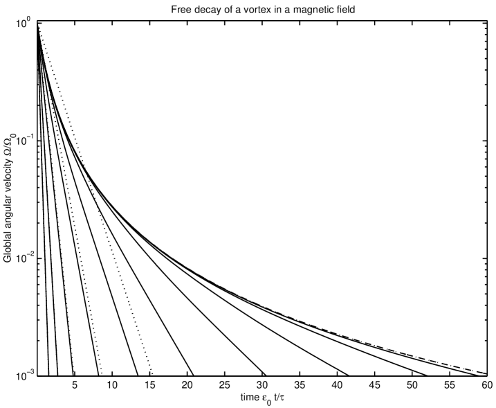
Figure 8: Free decay of a vortex in a magnetic field. Dash-doted lines: Bodewadt case ($A_{0}=0)$. Solid: numerical solution of (84) for Elsasser number equal to {0.00032, 0.001, 0.0032, 0.01, 0.032, 0.1, 0.32, 1, 3.16, 10 } (stronger decay when $A_{0}$ increases). Dotted lines: linear approximation (88) for $A_{0}$ in {0.1, 0.32, 3.16, 10}. The last two dotted lines cannot be distinguished from the fully non-linear solution.

The general equation (84) has been solved numerically for values of the initial Elsasser number in the range $10^{-3}\to 10^{3}$ (see figure 8). The approximation (88) turns out to be very accurate when $A_{0}$$\geqslant$1. Even for an initially dominant rotation, the decay becomes exponential when $A$ reaches a value of the order of $1$.

6 Conclusions

The first part of this work has provided some weakly non-linear analytical solutions to the semi-infinite Hartmann-Bödewadt problem, which provides a better approximation than the usual Ekman linear approximation. These new velocity profiles turn out to be quite close to the fully non-linear numerical solution (though they slightly underestimate the oscillating part of the profile), which justifies their use in further work. The numerical results are new as well, and together with the analytical solutions, they point out that the Bödewadt-Hartmann layer becomes very close to the simple Hartmann layer exponential profile as soon as the Elsasser number reaches a few units. The second part (sections 4 and 5) of this work tackles the problem of a forced or free vortex in a confined layer of fluid, in which the Bödewadt-Hartmann boundary layer is shown to have the same dynamics as in the semi-infinite problem. As the core flow directly depends on the quantities injected by the boundary layer into the core (vertical flow rate and vertical electric current), the results of the semi-infinite problem allows us to derive an expression for the core global angular velocity both in the case of a constant forcing and for the spin-down from some initial value of the rotation. In the latter case, it is found that meridian electric current and secondary flows essentially result in effects similar to friction, with a characteristic time varying from a linear Ekman layer characteristic friction time (when rotation dominates electromagnetic effects) to the Hartmann layer friction time (when electromagnetic effects dominates rotation).

Acknowledgements

The authors would like to thank René Moreau and Joël Sommeria for the fruitful discussions on this work.

References

- [1] D.J Acheson and R. Hide. Hydromagnetics in rotating fluids. Rep. Prog. Phys., 36:159–221, 1973.
- [2] C.J Stephenson. Magnetohydrodynamic fow between rotating coaxial disks. J. Fluid Mech, 38:335–352, 1969.
- [3] M. I. Loffredo. Extension of von Karman ansatz to magnetohydrodynamics. Mecanica, pages 81–86, 1986.
- [4] H. P. Greenspan. The theory of rotating fluids. Cambridge University Press, 1969.
- [5] P.J. Zandbergen and D. Dijkstra. Von karman swirling flows. Ann. Rev. Fluid. Mech., 19:465–491, 1987.
- [6] S.N. Curle and H.J. Davis. Modern Fluid Dynamics. Von Nostrand, 1968.
- [7] A. Pothérat, J. Sommeria, and R. Moreau. An effective two-dimensionnal model for MHD flows with tranverse magnetic field. J. Fluid. Mech., 424:75–100, 2000.
- [8] E. Grenier B. Desjardins, E. Dormy. Stability of mixed ekman-hartmann boundary layers. Nonlinearity, 12:181–199, 1999.
- [9] E. Grenier B. Desjardins, E. Dormy. Instability of mixed ekman-hartmann boundary layers with application to the fluid flow near the core mantle boundary. Physics of the Earth Planetary Interiors, 123:15–26, 2001.
- [10] P.H. Roberts. Introduction to Magnetohydrodynamics. Longmans, 1967.
- [11] P. A. Davidson. Swirling flow in axisymmeetric cavity of arbitrary profile driven by a rotating magnetic field. J. Fluid. Mech., 245:669–699, 1992.