Statistical properties of type D dispersing billiards

Abstract.

We consider dispersing billiard tables whose boundary is piecewise smooth and the free flight function is unbounded. We also assume there are no cusps. Such billiard tables are called type D in the monograph of Chernov and Markarian [9]. For a class of non-degenerate type D dispersing billiards, we prove exponential decay of correlation and several other statistical properties.

1. Introduction

Consider a collection of disjoint open sets on the torus $\mathbb{T}^{2}=\mathbb{R}^{2}/\mathbb{Z}^{2}$ (called scatterers in the sequel) with piecewise $C^{3}$ boundary which are locally convex with bounded from below curvature at regular points. We assume that there are no cusps. To define the Sinai billiard flow [16], let a point particle fly freely with constant speed on the complement of the scatterers (called the billiard table) and be subject to elastic collision upon reaching their boundaries. Depending on the geometry of the scatterers, the free flight time may or may not be bounded. A partial classification of dispersing billiard tables is given by [9] as follows: assume first that the boundary of the billiard table is $\mathcal{C}^{3}$. If the free flight is bounded, then the table is of type A, otherwise of type B. Now assume that the boundary of the billiard table is only piecewise $\mathcal{C}^{3}$. Points where the boundary is $\mathcal{C}^{3}$ are called regular. The finitely many non-regular points are called corner points. If the free flight is bounded, then the table is of type C, otherwise of type D. (In case of cusps, type E and F.) Statistical properties were first proven for type A billiards (see the central limit theorem in [3, 4, 5], exponential decay of correlations [18]). Next, type B tables were also extensively studied (see [2, 17, 7]). Although there are early works for types C and D [5], the more recent theory (such as the construction of Young towers [18]) was not studied in these classes until recently. For type C billiard tables, [11] proves the $m$-step expansion estimate, which together with other estimates (that can be proved as in type A) yield the statistical properties mentioned above. There are fewer results available in types D-F (in fact, these classes are labelled as ”hard” in [9])

It is standard that long free flights are only possible after a collision in a small vicinity of finitely many points, which we call boundary points of corridors. We now distinguish two classes of type D billiard tables: if all boundary points of corridors are regular, we say that the billiard table is of type D1, otherwise of type D2. The main result of the present work can be informally stated as follows.

Theorem 1.

Consider a billiard table of type D1 or type D2, in which case we also require that assumptions (A1) and (A2) hold. Then the correlation of bounded dynamically Hölder observables decay exponentially fast and the central limit theorem holds for such observables.

The precise definitions are given in Section 2. We note that some conditional results are available in the literaure, see e.g. the condition on complexity in [4]. Up to our best knowledge that condition on complexity is not known to hold generically and in fact is not verified for any specific billiard table. Our conditions (A1), (A2) hold on an open and dense set of billiard tables and furthermore given any billiard table it is easy to check whether they hold as they only depend on the boundary points of the corridors.

The rest of this paper is organized as follows. In Section 2 we collect the necessary background information needed in this work. None of the results of Section 2 are new. In Section 3 we state our main technical theorems. Theorem 2 implies Theorem 1 in type D1. Theorem 3 implies Theorem 1 in type D2. Section 4 contains the proof of Theorem 2. Section 5 contains the proof of Theorem 3. This proof is substantially more complex then that of Theorem 2 as we need a careful study of the geometry of long free flights in case of type D2 configurations. The proof of an important lemma is postponed to Section 6. In Section 7, we prove that the conditions (A1), (A2) hold on an open and dense set of billiard tables.

We mention that very recently there has been an increasing interest in the detailed description of possible orbits in infinite corridors in cases of hyperbolic billiards [1, 13] and in some similar hyperbolic systems with singularities [12].

2. Preliminaries

Here we review the preliminaries needed for our work. All results in this section are known, see [6, 8, 9]. More specific references will be given for the most important statements.

2.1. Billiards of type D

Let $\mathbb{T}^{2}$ be the $2$-torus and $\mathcal{D}\subset\mathbb{T}^{2}$ be a dispersing billiard table. That is, the complement of $\mathcal{D}$ consists of finitely many (say $d$) connected components $\mathcal{B}_{i}$ (called scatterers). For convenience we also label the scatterers. Each scatterer $i=1,...,d$ is bounded by a finite union of curves $\Gamma_{i,j}$, $j=1,...,J_{i}$. It is assumed that $\Gamma_{i,j}$ is a $\mathcal{C}^{3}$ curve, that is there is a $\mathcal{C}^{3}$ function $f_{i,j}:[0,1]\rightarrow\mathbb{T}^{2}$ which is a bijection between $[0,1]$ and $\Gamma_{i,j}$. Furthermore, $f_{i,j}(1)=f_{i,j+1}(0)$ where $j+1$ is interpreted modulo $J_{i}$ (that is, $f_{i,J_{i}}(1)=f_{i,1}(0)$). The endpoints of $\Gamma_{i,j}$ are called corner points, all other points of $\Gamma_{i,j}$ are regular points. We require that one of the first three one-sided derivatives at $f_{i,J_{i}}(1)$ differ from the corresponding derivative at $f_{i,1}(0)$, that is no regular point is labelled as corner point. We also require that the curvature of $\Gamma_{i,j}$ is positive with uniform upper and lower bounds at all regular points. The orientation of $\Gamma_{i,j}$ is assumed to be so that when following $\Gamma_{i,1}$, $\Gamma_{i,2}$, …, $\Gamma_{i,J_{i}}$, we follow clockwise orientation and $\mathcal{D}$ is to the left hand side. The region enclosed by $\Gamma_{i,1},...,\Gamma_{i,J_{i}}$ (a subset of $\mathbb{T}^{2}\setminus\mathcal{D}$) is one scatterer. If the boundary of the scatterer $i$ is $\mathcal{C}^{3}$ smooth, i.e. does not contain corner points, then the scatterer is necessarily strictly convex and $J_{i}=1$. We also assume no cusps, that is the tangent lines of $\Gamma_{i,j}$ and $\Gamma_{i,j+1}$ have an angle of at least $\alpha_{0}$ at their common endpoint $f_{i,j}(1)$. The interiors of $\Gamma_{i,j}$ are disjoint for all $i,j$. Furthermore, at each corner point exactly two curves meet and their angle is bounded from below by some positive constant. Any billiard table satisfying these assumptions is called admissible.

Given a corner point, let $\gamma$ be the angle between the two half tangent lines at it, measured at the interior of $\mathcal{D}$. The admissible property implies that $\gamma\neq 0$ for all corner points (the case $\gamma=0$ is called a cusp). We say that the corner point is convex if $0<\gamma\leq\pi$. Note that $\gamma=\pi$ is possible, in this case we assume that either the second or the third derivatives on the two sides of the corner points differ. We say that the corner point is concave if $\pi<\gamma<2\pi$ (noting that $\gamma=2\pi$ is impossible due to local convexity of the scatterers at regular points). See Figure 1.

Figure 1. A scatterer with a convex corner point (left) and a concave corner point (right)

Given two admissible billiard tables $\mathcal{D}_{1},\mathcal{D}_{2}$ with the same combinatorial data (that is the same number of scatterers $d$ and the same number of smooth pieces $J_{i}$, $i=1,..,d$), we define their distance as

$$d(\mathcal{D}_{1},\mathcal{D}_{2})=\inf_{\{f^{1}\},\{f^{2}\}}\max_{i,j}d_{\mathcal{C}^{3}}(f^{1}_{i,j},f^{2}_{i,j}),$$

where the infimum is taken over admissible parametrizations, i.e. collections of $\mathcal{C}^{3}$ functions $f^{k}_{i,j}$ so that $f^{k}_{i,j}$ is a bijection between $[0,1]$ and $\Gamma^{k}_{i,j}$ where $k=1,2$ indicates the two billiard tables. This makes the set of labelled admissible billiard tables with given combinatorial data a metric space $\bm{D}_{d,J_{1},...,J_{d}}$. Let $\bm{D}$ denote the space of all (labelled) admissible billiard tables, that is $\bm{D}=\cup_{d,J_{1},...,J_{d}}\bm{D}_{d,J_{1},...,J_{d}}$. The space $\bm{D}$ is also a metric space by defining the distance between two tables of different combinatorial data to be infinite (mind the labelling).

The billiard dynamics on a fixed admissible billiard table $\mathcal{D}$ prescribes the motion of a point particle that flies with constant speed $1$ in a given direction $v$ until it reaches the boundary $\partial\mathcal{D}$, where it undergoes an elastic collision (meaning the angle of reflection equals the angle of incidence). The phase space of the billiard flow is $\Omega=\mathcal{D}\times\mathcal{S}^{1}/\sim$, where $\sim$ means identifying pre-collisional and post-collisional data (that is, if $q\in\partial\mathcal{D}$ is a regular point, then $v$ and $-v$ are identified unless $v$ is tangent to $\partial\mathcal{D}$ at $q$. We will discuss the case of corner points in more detail later). We use the notation $(q,v)\in\Omega$ with $v$ being the velocity vector. We say that $\mathcal{D}$ is the configuration space and $q=\Pi_{\mathcal{D}}(q,v)$ is the configurational component of $(q,v)$. The billiard flow is denoted by $\Phi^{t}:\Omega\mapsto\Omega$ for every $t\in\mathbb{R}$.

Note that the dynamics may not be well defined upon reaching a corner point. Such trajectories have Lebesgue measure zero, so the definition of $\Phi$ on this set is irrelevant for physical properties. It is convenient, though, to define the flow to be possibly multi-valued upon reaching a corner point, corresponding to possible limit points of nearby regular orbits. One way of defining the flow is as follows. First, we say that a collision is improper if the trajectory can be approximated by trajectories missing the collision. In the case of smooth scatterers, an improper collision is the same as a grazing collision. In the case of a concave corner point, we may have an improper collision which is not grazing (such as a horizontal flight touching the corner point on the right of Figure 1). A proper collision is a collision that is not improper. For example, a vertical flight hitting the corner on the right of Figure 1 is proper, and nearby regular trajectories have two possible continuations. All trajectories hitting a convex corner point are proper. Furthermore, we may have a sequence of short flights near the convex corner point (also known as corner sequence), but the number of short collisions (the length of the corner sequence) is bounded due to the assumption that there are no cusps (see [6, Section 9]). Now given a point $(q,v)$, put $\tau(q,v)=\inf\{t>0:\Pi_{\mathcal{D}}\Phi^{t}(q,v)\in\partial\mathcal{D}\}$. Now assuming that $\lim_{t\nearrow\tau(q,v)}\Pi_{\mathcal{D}}\Phi^{t}(q,v)$ is a corner point $\tilde{q}\in\partial\mathcal{D}$, we define $\Phi^{\tau(q,v)}(q,v)$ as

$$\lim_{\varepsilon\searrow 0}\lim_{q^{\prime}\rightarrow q,v^{\prime}\rightarrow v}\Phi^{\tau(q,v)+\varepsilon}(q^{\prime},v^{\prime})$$

where $q^{\prime},v^{\prime}$ are points that can only experience collisions at regular points up to time $\tau(q,v)+\varepsilon$ and the second limit is to be interpreted as the set of all possible limit points. With this definition, $\Phi^{\tau(q,v)}(q,v)$ can take one or two values. This is trivial in case of concave corner points; for convex points see [9, Section 2.8]. The flow $\Phi^{t}$ preserves the Lebesgue measure $\nu$ on $\Omega$ (we assume by normalization that $\nu$ is a probability measure).

We will also study the billiard map. Let $\mathcal{M}$ be a cross-section of post-collisional points. Then $\mathcal{M}$ can be identified with a union of cylinders and rectangles. For any curve $\Gamma_{i,j}$, we define $\mathcal{M}_{i,j}=[a_{i,j},b_{i,j}]\times[-\pi/2,\pi/2]$ where $b_{i,j}-a_{i,j}=|\Gamma_{i,j}|$ and the intervals $[a_{i,j},b_{i,j}]$ are disjoint. If the scatterer $i$ is smooth (in this case necessarily $J_{i}=1$), then we identify the endpoints of the interval $[a_{i,1},b_{i,1}]$, so $\mathcal{M}_{i,1}$ becomes a cylinder. Finally, we put $\mathcal{M}=\cup_{i,j}\mathcal{M}_{i,j}$. Coordinates in $\mathcal{M}$ are denoted by $(r,\varphi)$: $r$ is arclength parameter along the boundary of the scatterer in clockwise direction; $\varphi$ is the angle of the postcollisional velocity and the normal to $\mathcal{D}$ at $q$ pointing into $\mathcal{D}$. The angle $\varphi$ is also measured in the clockwise direction with $\varphi\in[-\pi/2,\pi/2]$ (see [9, Figure 2.14]). The billiard map is denoted by $F:\mathcal{M}\rightarrow\mathcal{M}$. It preserves the physical invariant measure $\mu$ defined by $d\mu=C_{\mu}\cos\varphi drd\varphi$, where $C_{\mu}$ is a normalizing constant ($\mu$ is obtained as the projection of $\nu$ to the Poincaré section). The flow is now a suspension over the base map $F$ with roof function $\tau$, which is the free flight time. Note that $F$ can be multivalued at points when the next collision is at a corner point. The special case of unbounded free flight near a corner point will be discussed in the next section.

For ease of notation, we will identify $\mathcal{M}$ with a subset of $\Omega$ in the natural way. For example, we will write $\Pi_{\mathcal{D}}x$ for $x\in\mathcal{M}$.

2.2. Structure of corridors

Next we study corridors. We say that an admissible billiard table has infinite horizon if the free flight is unbounded. In this case, there are finitely many ”corridors”. A corridor $H$ by definition is a direction $v=v_{H}\in[0,\pi)$ and a connected subset $Q_{H}$ of $\mathcal{D}$ with non-empty interior

(1) $$Q_{H}=\{q\in\mathcal{D}:\forall t\in\mathbb{R}:q+tv\in\mathcal{D}\}.$$

There are only finitely many corridors (see [9, Exercise 4.51]). Let us say that an admissible billiard table is of type D1 if all corridors are bounded by grazing orbits at regular points (such orbits are necessarily periodic). In other words, a billiard table is regular if no corner point is in the corridors. If the billiard table is of type D but not of type D1, then we call it type D2. We say that an admissible billiard table is simple if for all corridors $H$, $B_{H}:=\partial Q_{H}\cap\partial\mathcal{D}$ consist of exactly $2$ points, one on both sides of $Q_{H}$, that is $B_{H}=\{q_{H,l},q_{H,r}\}$. Here, $l$ and $r$ stand for left and right points, when viewed from the direction $v$. For simple billiard tables, we consider the four points in $\mathcal{M}$, whose trajectory up to the next collision projects onto $\partial Q_{H}$ in the configuration space. The set of these four points is denoted by

(2) $$A_{H}=\{(r_{H,l,1},\varphi_{H,l,1}),(r_{H,l,2},\varphi_{H,l,2}),(r_{H,r,1},\varphi_{H,r,1}),(r_{H,r,2},\varphi_{H,r,2})\}.$$

We will say that the elements of $A_{H}$ are boundary points of the corridor $H$. Note that if $q_{H,s}$ is a regular point (for $s=l,r$), then $r_{H,s,1}=r_{H,s,2}$ corresponds to a vertical line segment in the interior of $\mathcal{M}_{i,j}$. On the other hand, if $q_{H,l}$ is a corner point, then $r_{H,l,1}$ corresponds to the right side of $\mathcal{M}_{i,j}$ and $r_{H,l,2}$ corresponds to the left side of $\mathcal{M}_{i,j+1}$ (and vice versa for the right boundary: if $q_{H,r}$ is a corner point, then $r_{H,r,2}$ corresponds to the right side of $\mathcal{M}_{i^{\prime},j^{\prime}}$ and $r_{H,r,1}$ corresponds to the left side of $\mathcal{M}_{i^{\prime},j^{\prime}+1}$). In this case and with a slight abuse of notation, we will also say that the elements of $A_{H}$ are corner points. Note that whenever $q_{H,s}$ is a corner point, it is necessarily concave. See Figure 2 for a typical arrangement in the case that both sides are bounded by a corner point (for simplicity, we depict $i=j=j^{\prime}=1$, $i^{\prime}=2$, $v$ is horizontal, so by convention pointing to the right). The figure represents a part of the scatterer configuration lifted from $\mathbb{T}^{2}$ to $\mathbb{R}^{2}$. The point $q_{H,r}=\Gamma_{1,1}\cap\Gamma_{1,2}$ is the corner point on the bottom left as well as the bottom right of the figure. The two corresponding signed angles $\varphi_{H,r,k}$, $k=1,2$ are between the dashed lines (normals to the curves) and the lower dotted line. Similarly, observe the left boudary of the corridor on the top part of the figure. In this paricular case, we have $\varphi_{H,r,1}>0$, $\varphi_{H,r,2}<0$, $\varphi_{H,l,1}<0$, $\varphi_{H,l,2}>0$ although these signs may be different for other corridors bounded by two corner points. Note that

(3) $$F(r_{H,r,1},\varphi_{H,r,1})=(r_{H,r,2},-\varphi_{H,r,2})$$

which corresponds to an improper collision. According to our definition, $\Phi^{\tau(r_{H,r,1},\varphi_{H,r,1})}(r_{H,r,1},\varphi_{H,r,1})$ takes two values: $(r_{H,r,2},-\varphi_{H,r,2})$ and $(r_{H,r,1},\varphi_{H,r,1})$ (where we identified $\mathcal{M}$ with a subset of $\Omega$). This corresponds to an improper collision and so by our terminology (3) holds. There are two possible types of free flights from regular points close to $(r_{H,r,1},\varphi_{H,r,1})$. One possibility is a flight of bounded length, terminating on $\Gamma_{1,1}$. For such points $(q,v)$, $F(q,v)$ is close to $(r_{H,r,2},-\varphi_{H,r,2})$. The other possibility is a very long flight in the corridor which eventually terminates on $\Gamma_{2,2}$. For such points $(q,v)$, $F(q,v)$ is close to $(r_{H,l,2},-\varphi_{H,l,2})$. The local geometry of such orbits will be studied more carefully later.

Figure 2. A simple corridor bounded by two corner points

Now we define $A=\cup_{H\text{ corridors}}A_{H}$. With these notations, we are ready to introduce our assumptions

• $\mathcal{D}$ is simple.

• For any $(r,\varphi)\in A$, if $r$ corresponds to a corner point, then $|\varphi|\neq\pi/2$.

It seems likely that our results remain true if we remove (A1) and (A2) but the proof becomes more complicated so we assume them for convenience.

2.3. Definitions

We will denote by $C$ any constant only depending on $\mathcal{D}$, whose explicit value is irrelevant. In particular, the value of $C$ may change from line to line.

The billiard map $F$ is hyperbolic and ergodic. In particular, there exists uniformly transversal families of stable and unstable cones. Specifically, there are cones $\mathcal{C}^{u/s}_{x}$ for every $x\in\mathcal{M}$ so that $D_{x}F(\mathcal{C}^{u}_{x})\subset F(\mathcal{C}^{u}_{F(x)})\cup\{0\}$ and $D_{x}F^{-1}(\mathcal{C}^{s}_{x})\subset F(\mathcal{C}^{s}_{F^{-1}(x)})\cup\{0\}$. Furthermore, there is a positive number $a$ so that for any $x\in\mathcal{M}$ and any $(dr_{1},d\varphi_{1})\in\mathcal{C}^{u}_{x}$, $(dr_{2},d\varphi_{2})\in\mathcal{C}^{s}_{x}$, we have $a\leq d\varphi_{1}/dr_{1}$ and $d\varphi_{2}/dr_{2}\leq-a$. Furthermore, at least one of the following two inequalities hold: $d\varphi_{1}/dr_{1}\leq a^{-1}$, $-a^{-1}\leq d\varphi_{2}/dr_{2}$ (see [6, Section 9]. We note that all of these inequalities hold when there are no corner points.) Vectors in $\mathcal{C}^{u}_{x}$ ($\mathcal{C}^{s}_{x}$) are called unstable (stable). It follows that the exists some number $\gamma>0$ so that at any point $x\in\mathcal{M}$, the angle between any stable and unstable vector is bounded from below by $\gamma$ and no horizontal vector (that is $d\varphi=0$) can be in the stable/unstable cones. The standard way of defining the stable/unstable cones is as the $DF$/$DF^{-1}$ image of the cones $drd\varphi\geq 0$. We will briefly refer to these properties as transversality.

Hyperbolicity needs to be understood in the sense that for almost every point there is an unstable and a stable manifold through this point, however they can be arbitrarily short. This is due to the singularities. The hyperbolicity is uniform in the sense that there are constants $C_{\#}$ and $\Lambda_{*}>1$ so that for any $n\geq 1$, for every unstable vector $u$,

(4) $$\|DF^{n}(u)\|\geq C_{\#}\Lambda_{*}^{n}\|u\|$$

and for any stable vector $v$,

$$\|DF^{-n}(v)\|\geq C_{\#}\Lambda_{*}^{n}\|v\|.$$

Let us write

$$S_{0}=\cup_{i,j}\Gamma_{i,j}\times\{\pm\pi/2\},\quad V_{0}=\cup_{i}\cup_{j}\partial\Gamma_{i,j}\times[\pi/2,\pi/2],$$

that is $S_{0}$ is the set of grazing collisions and $V_{0}$ is the set of collisions at the corner points, and $R_{0}=S_{0}\cup V_{0}$. Furthermore, let $R_{m,n}=\cup_{l=m}^{n}F^{l}R_{0}$. Then for any $n\geq 1$ (including $n=\infty$), the singularity set of $F^{n}$ is $R_{-n,0}$ and the singularity set of $F^{-n}$ is $R_{0,n}$. Furthermore, as usual, we introduce secondary (artificial) singularities

$$\hat{S}_{\pm k}=\{(r,\phi):\phi=\pm\pi/2\mp k^{-2}\}$$

for some $k\geq k_{0}$ to control distortion. We denote

$$\mathbb{H}_{0}={\{r,\varphi\in\mathcal{M}:-\pi/2-k_{0}^{-2}\leq\varphi\leq\pi/2-k_{0}^{-2}\}}$$

$$\mathbb{H}_{k}={\{r,\varphi\in\mathcal{M}:\pi/2-k^{-2}\leq\varphi\leq\pi/2-(k+1)^{-2}\}}$$

$$\mathbb{H}_{-k}={\{r,\varphi\in\mathcal{M}:-\pi/2+(k+1)^{-2}\leq\varphi\leq-\pi/2+k^{-2}\}}.$$

The extended set of singularities is

$$R_{0}^{\mathbb{H}}=S_{0}^{\mathbb{H}}\cup V_{0},\text{ where }S_{0}^{\mathbb{H}}=S_{0}\cup(\cup_{k\geq k_{0}}\hat{S}_{\pm k})$$

and likewise $R_{n,m}^{\mathbb{H}}=\cup_{l=m}^{n}F^{l}R_{0}^{\mathbb{H}}$. We say that a $C^{2}$ curve in $W\subset\mathcal{M}$ is unstable if at every point $x\in W$, the tangent line $T_{x}W$ is in the unstable cone, and $W$ has a uniformly bounded curvature and is disjoint to $R_{0}$ (except possibly for its endpoints). We say that an unstable curve is homogeneous if it lies entirely in $\mathbb{H}_{k}$ for some $k$ ($k=0$ or $|k|\geq k_{0}$). It is useful to think about unstable curves as smooth curves in the northeast-southwest direction on $\mathcal{M}$.

As in [8, section 4], we say that $\ell=(W,\rho)$ is a standard pair if $W$ is a homogeneous unstable curve and $\rho$ is a probability measure supported on $W$ that satisfies

$$\left|\log\frac{d\rho}{dLeb}(x)-\log\frac{d\rho}{dLeb}(y)\right|\leq C_{0}\frac{|W(x,y)|}{|W|^{2/3}}.$$

Note that there is some constant $C$ so that for any standard pair $\ell=(W,\rho)$ and for any $x,x^{\prime}\in W$

(5) $$e^{-C|W|^{1/3}}\leq\frac{\rho(x)}{\rho(x^{\prime})}\leq e^{C|W|^{1/3}}.$$

The image of a standard pair is a weighted average of standard pairs. More precisely, if $\ell=(W,\rho)$ is a standard pair and $\nu_{\ell}$ is the measure on $W$ with density $\rho$, then $F(W)=\cup_{i}W_{i}$, where $W_{i}$ are homogeneous unstable curves and $F_{*}(\nu_{\ell})=\sum_{i}c_{i}\nu_{\ell_{i}}$, where $\ell_{i}=(W_{i},\rho_{i})$ are standard pairs (see [8, Proposition 4.9 ]). We will also write $F_{*}({\ell})=\sum_{i}c_{i}{\ell_{i}}$.

Substandard families are weighted averages of standard pairs where the sum of the weights is $\leq 1$. That is, $\mathcal{G}=((W_{\alpha},\rho_{\alpha})_{\alpha\in\mathfrak{A}},\lambda)$ is a substandard family if $(W_{\alpha},\rho_{\alpha})$’s are standard pairs and $\lambda$ is a subprobability measure on $\mathfrak{A}$. We assume that the $W_{\alpha}$’s are disjoint. Given a substandard family $\mathcal{G}$, it induces a measure $\nu_{\mathcal{G}}$ on $\mathcal{M}$ by

$$\nu_{\mathcal{G}}(B)=\int_{\alpha\in\mathfrak{A}}\nu_{\alpha}(B\cap W_{\alpha})d\lambda(\alpha)\text{ for }B\subset\mathcal{M}\text{ Borel sets, }$$

where $\nu_{\alpha}$ is the measure on $W_{\alpha}$ with density $\rho_{\alpha}$. In case $\lambda_{\mathcal{G}}$ is a probability measure, we call $\mathcal{G}$ a standard family. Now given a point $x\in W_{\alpha}$, denote by $r_{\mathcal{G}}(x)$ the distance between $x$ and the closest endpoint of $W_{\alpha}$ (measured along $W_{\alpha}$ with respect to arclength). We introduce the notion of the $\mathcal{Z}_{q}$ function for $q\in(0,1]$ by

$$\mathcal{Z}_{q}(\mathcal{G})=\sup_{\varepsilon>0}\frac{\nu_{\mathcal{G}}(r_{\mathcal{G}}<\varepsilon)}{\varepsilon^{q}}.$$

For example if $\mathcal{G}$ consists of only one standard pair $(W,\rho)$, then

(6) $$\mathcal{Z}_{q}(\mathcal{G})\sim 2^{q}/|W|^{q}$$

as $|W|\rightarrow 0$. A fundamental fact about the class of standard families is that they are preserved under iterations of the map $F$.

Given a homogeneous unstable curve $W$, its image $F^{m}(W)$ will consist of a collection of homogeneous unstable curves $W_{i}$. For each $i$, let $\Lambda_{i}=\Lambda_{i,m}$ be the minimal expansion factor of $F^{m}$ on $F^{-m}W_{i}$. We say that the $m$-step expansion holds if

$$\lim_{\delta\rightarrow 0}\sup_{W:|W|<\delta}\sum_{i}\frac{1}{\Lambda_{i,m}}<1,$$

where the supremum is taken over homogeneous unstable curves. We note that the above limit is traditionally written as $\liminf$, however the sequence as $\delta\rightarrow 0$ is non-increasing and bounded below, so the limit always exists.

For given $n$, let $\xi^{n}$ be the partition of $\mathcal{M}\setminus R_{0,n}^{\mathbb{H}}$ into connected components. Now the forward separation time of points $x,y\in\mathcal{M}$, denoted by $s_{+}(x,y)$, is defined as the smallest $n$ so that $x$ and $y$ belong to different partition elements of $\xi^{n}$. Likewise, we define $s_{-}(x,y)$ as the backward separation time. We say that $f:\mathcal{M}\rightarrow\mathbb{R}$ is dynamically Hölder if there are constants $C=C(f)$ and $\vartheta=\vartheta(f)<1$ so that for any $x,y$ on the same unstable manifold $W^{u}$,

$$|f(x)-f(y)|\leq C\vartheta^{s_{+}(x,y)}$$

and for any $x,y$ on the same stable manifold $W^{s}$,

$$|f(x)-f(y)|\leq C\vartheta^{s_{-}(x,y)}.$$

We will write $a_{n}\sim b_{n}$ if $\lim_{n\rightarrow\infty}a_{n}/b_{n}=1$ and $a_{n}\approx b_{n}$ if there are is a constant $C$ so that $1/C\leq a_{n}/b_{n}\leq C$ for all $n$.

3. Results

Now we can state our results.

Theorem 2.

For all type D1 billiard tables there is some $m_{0}$ so that the $m_{0}$-step expansion holds.

Theorem 3.

For all type D2 billiard tables satisfying (A1) and (A2) and for all $q\in(0,1)$ we have the following. There are constants $M\in\mathbb{N}$, $\varkappa<1$ and $\delta_{0}>0$ so that for any standard pair $\ell=(W,\rho)$ with $|W|<\delta_{0}$, $\mathcal{Z}_{q}(F^{M}_{*}(\ell))<\varkappa\mathcal{Z}_{q}(\ell)$.

Theorem 4.

The set of billiard tables satisfying (A1) and (A2) is open and dense in $\bm{D}$.

Proof of Theorem 1 assuming Theorems 2, 3.

In the case of type D1 billiard tables, the key estimate is the $m_{0}$-step expansion, provided by Theorem 2. Once it is established, the exponential decay of correlations and the central limit theorem follow from the theory developed in [6] as it was also noted in case of type C billiards in [11].

In the case when the assumptions (A1) and (A2) are satisfied, the result follows from [10]. In that work, the exponential decay of correlation follows from some abstract assumptions denoted by (H1) - (H5). In our case, assumptions (H1)-(H4) are standard as is usual for billiards (see e.g. [6, section 9]). We do not know how to prove (H5) (see Remark 8 below) however we have Theorem 3 instead. In the proof of [10], (H5) is only used to derive the growth lemma (see [10, Lemma 3(a)]) which is standard once our Theorem 3 holds. That being said, we can replace (H5) by Theorem 3 and conclude the result of Theorem 1. ∎

Remark 5.

Under the same assumptions as Theorm 1, several other results follow immediately from the abstract theory. Indeed, a ”magnet” is constructed in [10] which implies the existence of a Young tower [18] with exponential return times. Thus the central limit theorem [18], large deviation principles [15], almost sure invariance principle, law of iterated logarithm [7, 14], etc. follow.

Remark 6.

It is important to note that the test functions in the setup of Theorem 1 and Remark 5 are assumed to be bounded and dynamically Hölder. Important functions of interest are the free flight time $\tau:\mathcal{M}\rightarrow\mathbb{R}$ and the displacement vector $\kappa:\mathcal{M}\rightarrow\mathbb{R}^{2}$ defined as $\Pi_{\mathcal{D}}(F(x))-\Pi_{\mathcal{D}}(x)$, lifted to the universal cover $\mathbb{R}^{2}$. Both of these functions are dynamically Hölder but unbounded. In particular, we do not claim the central limit theorem for the position of the billiard particle in the periodic extension of $\mathcal{D}$ from $\mathbb{T}^{2}$ to $\mathbb{R}^{2}$ (also known as Lorentz gas). In fact, we expect that the this position will converge to the normal distribution under the scaling $\sqrt{t\log t}$ (where $t$ is continuous time in case the flow is considered, and collision time in case of the map) as in [17], but we do not study this question here.

4. Proof of Theorem 2

The proof of Theorem 2 is based on similar proofs for type C as in [11] and type B as in [9]. As such, we only give detailed arguments at places where our proof differs from these references and otherwise cite the necessary lemmas from [9, 11].

First we review the structure of corridors and singularities, see [9, Section 4.10] for details. Let us fix a regular billiard table. There are finitely many points,

$$A=\{x_{h}=(r_{h},\varphi_{h}),h=1,...,h_{\max},\varphi_{h}=\pm\pi/2\}$$

that are periodic and whose trajectories bound the corridors. The singularity structure of $F$ and $F^{-1}$ near $x_{h}$ is as follows. There are infinitely many singularity curves accumulating at $x_{h}$. Specifically, there are connected components $D^{+}_{h,n}$ for $n\geq 1$ in a neighborhood of $x_{h}$ so that $F$ is smooth on $D^{+}_{h,n}$ and the trajectories of the points in $D^{+}_{h,n}$ pass by $n$ copies of the given scatterer before the next collision. Likewise, $D^{-}_{h,n}$ is a set on which $F^{-1}$ is continuous, and $F(D^{+}_{h,n})=D^{-}_{h^{\prime},n}$ for some $h^{\prime}$. The size of $D^{+}_{h,n}$ is $\approx n^{-2}$ in the unstable direction and $\approx n^{-1/2}$ in the stable direction. Likewise, the size of $D^{-}_{h,n}$ is $\approx n^{-1/2}$ in the unstable direction and $\approx n^{-2}$ in the stable direction. Consequently, $D^{-}_{h,n}$ intersects with $\mathbb{H}_{k}$ if $|k|\geq Cn^{1/4}$. The rate of expansion of $F$ on $D^{+}_{h,n}\cap F^{-1}(\mathbb{H}_{k})$ is $\approx nk^{2}$.

We start by the following

Lemma 1.

There is a constant $C$ so that for any unstable curve $W$ and for any homogeneous connected component $W^{\prime}\subset F(W)$, we have

$$|W^{\prime}|\leq C|W|^{1/3}.$$

Proof.

Let $N$ be an arbitrary positive integer. If $W\not\subset\cup_{h}\cup_{n\geq N}D^{+}_{h,n}$, then the stronger bound $|W^{\prime}|\leq C|W|^{1/2}$ holds with $C=C(N)$ by [9, Exercise 4.50]. Let us assume now that $W\subset\cup_{n\geq N}D^{+}_{h,n}$. We can also assume that there is some $n$ so that $W\subset D^{+}_{h,n}$. Indeed, for any connected component $W^{\prime}\subset F(W)$, by connectedness, there is some $n=n_{W^{\prime}}$ so that $F^{-1}(W^{\prime})\subset D^{+}_{h,n}$. Restricting $W$ to $D^{+}_{h,n_{W^{\prime}}}$ will decrease the length of $W$ but not change the length of $W^{\prime}$. Thus it is enough to prove the lemma when $W$ is replaced by $W\cap D^{+}_{h,n_{W^{\prime}}}$.

Since $W^{\prime}$ is a homogeneous unstable curve, there is some $k$ so that $W^{\prime}\subset\mathbb{H}_{\pm k}$. We can also assume that $F(W)=W^{\prime}$. Indeed, if $W^{\prime}\subset F(W)$, the proof is easier as $|F(W)|\geq|W^{\prime}|$. By the discussion right before the lemma, we have $|W^{\prime}|/|W|\approx nk^{2}$. Now extend $W$ smoothly to a longer unstable curve $\bar{W}$ so that $\bar{W}^{\prime}=F(\bar{W})$ is maximal with $\bar{W}^{\prime}\subset\mathbb{H}_{\pm k}$, i.e. the two endpoints of $\bar{W}^{\prime}$ belong to $\partial\mathbb{H}_{\pm k}$. Then $|\bar{W}^{\prime}|/|\bar{W}|\approx|W^{\prime}|/|W|\approx nk^{2}$. Recalling that $|k|>n^{1/4}$, we find $|\bar{W}^{\prime}|\leq C|\bar{W}|k^{6}$. Next, by transversality, we have $|\bar{W}^{\prime}|\approx|k|^{-3}$ and so $|\bar{W}^{\prime}|\leq C|\bar{W}|^{1/3}.$ We conclude

$$|W^{\prime}|\leq C|W|\frac{|\bar{W}^{\prime}|}{|\bar{W}|}\leq C|W||\bar{W}|^{-2/3}\leq C|W|^{1/3}.$$

∎

Remark 7.

In the case of finite horizon if we do not require $W^{\prime}$ to be homogeneous, we have $|W^{\prime}|\leq|W|^{1/2}$ by [9, Exercise 4.50]. Similarly to the above proof, one can show that in case of finite horizon and if $W^{\prime}$ is required to be homogeneous, then $|W^{\prime}|\leq|W|^{3/5}$ holds. Furthermore, in the case of infinite horizon if $W^{\prime}$ is not required to be homogeneous, then the weaker bound $|W^{\prime}|\leq|W|^{1/4}$ holds. Since we will not use these bounds, the proofs are omitted.

We will also need an estimate on the growth of the free flight function along orbits, which is provided by the next lemma.

Lemma 2.

There are constants $\Cl{c:conseclongflight},t_{0},t_{1}$ only depending on $\mathcal{D}$ so that for any point $x\in\mathcal{M}$ with $\tau(x)>t_{1}$, there are two possibilities:

• either $\tau(F(x))\in[\Cr{c:conseclongflight}^{-1}\sqrt{\tau(x)},\Cr{c:conseclongflight}(\tau(x))^{2}]$

• or $\tau(F(x))<t_{0}$ in which case $\tau(F^{2}(x))\in[\Cr{c:conseclongflight}^{-1}\sqrt{\tau(x)},\Cr{c:conseclongflight}(\tau(x))^{2}]$.

We don’t give a formal proof of Lemma 2, as the first case was proved in [17, Proposition 9] and the second case is similar. Instead, we give an explanation. A long flight needs to happen in a corridor, e.g. in the northeast direction in a horizontal corridor with an angle $\alpha\approx 1/\tau(x)$. Now let $P,P^{\prime}\in\partial\mathcal{D}$ be two consecutive points on the boundary of the corridor (see Figure 3) with $P\in\partial\mathcal{B}$, $P^{\prime}\in\partial\mathcal{B}^{\prime}$ (here $\mathcal{B}=\mathcal{B}_{i}+m$ and $\mathcal{B}^{\prime}=\mathcal{B}_{i}+m^{\prime}$ for some $i=1,...,d$ and $m,m^{\prime}\in\mathbb{Z}^{2}$). The free flight of $x$ will intersect the line segment $(P,P^{\prime})$. Let $Q,Q^{\prime}$ be two more points on this line segment with $P<Q<Q^{\prime}<P^{\prime}$, where $X<Y$ means that $Y$ is to the right of $X$. Here $Q^{\prime}$ is defined so that the line segment with angle $\alpha$ through $Q^{\prime}$ is tangent to $\mathcal{B}$ and $Q$ is defined by the property that a billiard particle travelling with angle $\alpha$ through $Q$ first collides with $\mathcal{B}$ and then experiences a grazing collision on $\mathcal{B}^{\prime}$.

Let $R$ denote the point where the free flight, starting from $x$, crosses $(P,P^{\prime})$. If $P\leq R<Q$, then $\tau(F(x))\in[\tau(x),\Cr{c:conseclongflight}(\tau(x))^{2}]$. If $Q\leq R\leq Q^{\prime}$, then $\tau(F(x))<\|m^{\prime}-m\|$ and $\tau(F^{2}(x))\in[\Cr{c:conseclongflight}^{-1}\sqrt{\tau(x)},\Cr{c:conseclongflight}(\tau(x))^{2}]$. Finally, if $Q^{\prime}<R<P^{\prime}$, then $\tau(F(x))\in[\Cr{c:conseclongflight}^{-1}\sqrt{\tau(x)},\tau(x))$. Also note that the last case is the typical one in the sense that $\|P-Q^{\prime}\|\approx 1/\tau(x)$.

Figure 3 represents the two cases of Lemma 2. The dashed line is a reference trajectory through $Q^{\prime}$. The solid line is a trajectory with $Q^{\prime}<R<P^{\prime}$ and the dash-dotted line is a trajectory with $Q<R<Q^{\prime}$. (Note that for the sake of legibility, this image doesn’t exactly reflect how small the angles would be.)

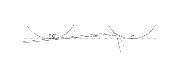
Figure 3. Collisions after a long flight

Now fix some $\varepsilon_{0}>0$, $n_{0}$ and $\bar{\tau}$ so that the following is true: For any point $x=(r,\varphi)\in\mathcal{M}$ that has a free flight longer than $\bar{\tau}$, there is some $h=1,...,h_{\max}$ so that $d(x,x_{h})<\varepsilon_{0}$ and $x\in D^{+}_{h,n}$ for some $n\geq n_{0}$. Furthermore, the trajectory of $x$ under the billiard flow until the next collision avoids the $\varepsilon_{0}$ neighborhood of all corner points in $\mathbb{T}^{2}$.

Let us write $\mathcal{M}_{\mathfrak{n}}=\mathcal{M}\setminus\cup_{h=1}^{h_{\max}}\cup_{n\geq\mathfrak{n}}D^{+}_{h,n}$ and $\mathcal{M}_{m,\mathfrak{n}}=\cap_{l=0}^{m}F^{-l}\mathcal{M}_{\mathfrak{n}}$. Note that for $m$ fixed and for $\mathfrak{n}$ large enough, we have

(7) $$\mathcal{M}_{(\hat{c}\mathfrak{n})^{1/(2^{m})}}\subset\mathcal{M}_{m,\mathfrak{n}}\subset\mathcal{M}_{\mathfrak{n}}.$$

Indeed, the first inequality follows from Lemma 2 and the second one is trivial.

Following [11], we introduce the following definitions. Let $W$ be a homogenenous unstable curve and $W_{i,m}$ the homogeneous components (H-components) of $F^{m}(W)$. We say that $W_{i,m}$ is $m$-regular if $F^{-l}(W_{l,m})\in\mathbb{H}_{0}$ for all $0\leq l<m$. If $W_{i,m}$ is not $m$-regular, it is called $m$-nearly grazing.

Given some $\mathfrak{n}$, $m$ and $z\in\mathcal{M}_{m,\mathfrak{n}}$, we define $\mathcal{K}_{m,\mathfrak{n}}^{reg}(z)$ as the number of connected components of $\mathcal{M}^{\prime}\subset\mathcal{M}_{\mathfrak{n}}\setminus R_{0,m}^{\mathbb{H}}$ so that the closure of $\mathcal{M}^{\prime}$ contains $z$ and some (and consequently all) points $x\in\mathcal{M}^{\prime}$ satisfy

(8) $$F^{l}(z)\in\hat{\mathbb{H}}_{0}\text{ for all }l=0,...,m,$$

where

$$\hat{\mathbb{H}}_{0}:=\mathbb{H}_{0}\cup\mathbb{H}_{k_{0}}\cup\mathbb{H}_{-k_{0}}.$$

Let

$$\mathcal{K}_{m}^{reg}=\sup_{\mathfrak{n}\geq 1}\sup_{z\in\mathcal{M}_{m,\mathfrak{n}}}\mathcal{K}_{m,\mathfrak{n}}^{reg}(z)$$

Now we have

Lemma 3.

There is some $\Xi$ depending only on $\mathcal{D}$ (and in particular not depending on $k_{0}$) so that

$$\mathcal{K}_{m}^{reg}=\sup_{\mathfrak{n}\geq 1}\sup_{z\in\mathcal{M}_{\mathfrak{n}}}\mathcal{K}_{m,\mathfrak{n}}^{reg}(z)\leq\Xi(m+1)$$

Proof.

By (7), the first equality follows. The inequality follows from [11, Lemma 3.5]. Although that lemma is only proved in the case of finite horizon, the proof applies in our case as well. Let us fix $\mathfrak{n}_{0}=\max\{n_{0},Ck_{0}^{4}\}$. Then the proof of [11] implies $\sup_{z\in\mathcal{M}_{\mathfrak{n}_{0}}}\mathcal{K}_{m,\mathfrak{n}_{0}}^{reg}(z)\leq\Xi(m+1)$. We just need to replace $\tau_{\max}$ by $\bar{\tau}$ in Lemma 3.6; in particular $\Xi=4\bar{\tau}/\tau_{*}+6$ works, where $\tau_{*}$ is the length of the minimal free flight between two improper collisions (a geometric constant only depending on $\mathcal{D}$). Indeed, whenever $\tau(x)>\bar{\tau}$ (this can happen if $\mathfrak{n}>n_{0}$), the trajectory up to the next collision avoids the $\varepsilon_{0}$ neighborhood of the corner points by the choice of $n_{0}$, so Lemma 3.6 remains valid. Now if $\mathfrak{n}>\mathfrak{n}_{0}$, then by the choice of $\mathfrak{n}_{0}$ and by Lemma 2, all points $z\in\mathcal{M}_{m,\mathfrak{n}}\setminus\mathcal{M}_{m,\mathfrak{n}_{0}}$ satisfy $F(z)\in{\mathbb{H}}_{k}$ for some $k$ with $|k|>k_{0}$. Thus $\mathcal{K}_{m,\mathfrak{n}}^{reg}(z)=0$.

∎

Let $k_{0}$ be fixed and let $K_{m}^{reg}(W)$ denote the number of $m$-regular H-components of $F^{m}(W)$. Then we have

Lemma 4.

There exists some $m_{0}$ only depending on $\mathcal{D}$ so that for any $k_{0}$,

$$\lim_{\delta\rightarrow 0}\sup_{W:|W|<\delta}K_{m_{0}}^{reg}(W)<\frac{1}{3}C_{\#}\Lambda_{*}^{m_{0}}$$

where $C_{\#}$ and $\Lambda_{*}$ are defined by (4).

Proof.

This lemma is proved as [11, Lemma 2.12]. We fix $m_{0}$ so that $\Xi(m_{0}+1)<\frac{1}{3}C_{\#}\Lambda_{*}^{m_{0}}$. Now since $k_{0}$ is fixed, we can choose $n_{1}>\max\{n_{0},k_{0}^{4}\}$. Then as in Lemma 3, if $z\notin\mathcal{M}_{m_{0},n_{1}}$, then $F(z)\in\mathbb{H}_{k}$ for $|k|>k_{0}$, so the H-component $W^{\prime}\subset F^{m_{0}}(W)$ containing $F^{m_{0}}(z)$ must be $m_{0}$-nearly grazing. Once $n_{1}$ is fixed, there are only finitely many points $\mathcal{Z}=\{z_{1},...,z_{Z}\}$ where $\mathcal{K}_{m_{0},n_{1}}^{reg}(z)>2$. By choosing $\delta=\delta(n_{1})$ small, we can assume that our curve $W$ is only close to one of these points and so by transversality and by the fact that we used $\hat{\mathbb{H}}_{0}$ in (8), we find $K_{m_{0}}^{reg}(W)\leq\mathcal{K}_{m_{0}}^{reg}$, which by Lemma 3 completes the proof. ∎

Next, we bound the contribution of nearly grazing components for $m=1$.

Lemma 5.

For any $\varepsilon>0$ there exists $k_{0}$ so that

$$\lim_{\delta\rightarrow 0}\sup_{W:|W|<\delta}\sum^{*}_{i}\frac{1}{\Lambda_{i,1}}<\varepsilon,$$

where $\sum^{*}$ means that the sum is restricted to nearly grazing H-components $W_{i,1}$.

Proof.

This lemma is analogous to [11, Lemma 2.13] but the proof differs substantially as the free flight now is unbounded. However, we can use [9, Remark 5.59].

Let us write $W_{1}=W\setminus\mathcal{M}_{n_{0}}$ and $W_{2}=W\cap\mathcal{M}_{n_{0}}$. Let $S^{*j}$ be the sum corresponding to the images of $W_{j}$ for $j=1,2$. As before, for any $k_{0}$ there exists some $\delta>0$ so that if $|W|<\delta$, then $F(W_{1})$ have at most $L=\bar{\tau}/\tau_{\min}+2$ connected components. Each of these components could be further cut by secondary singularities, so $S^{*1}\leq L\sum_{k\geq k_{0}}Ck^{-2}\leq CLk_{0}^{-1}$ which is less then $\varepsilon/2$ assuming that $k_{0}>2CL/\varepsilon$. For any fixed $k_{0}$ and $n_{0}$, we can make $S^{*2}\leq\varepsilon/2$ by further reducing $\delta$ if needed, exactly as in [9, Remark 5.59]. ∎

Now Theorem 2 follows from Lemmas 3, 4 and 5 as in [11]. Note that there is a typo at the middle of page 1231 in [11] as one only has

(9) $$\mathcal{L}_{n+m}(W)\leq\sum_{i}\frac{1}{\Lambda_{i,n}}\mathcal{L}_{m}(W_{i,n}),$$

where

(10) $$\mathcal{L}_{n}(W)=\sum_{i}\frac{1}{\Lambda_{i,n}}$$

(and the equation in (9) may not hold), but this is enough since Theorem 2 only gives an upper bound.

5. Proof of Theorem 3

By (A1) and (A2), we can group the corridors into three categories: $H\in\mathcal{H}_{1}$ if $H$ is bounded by two regular points, $H\in\mathcal{H}_{2}$ if $H$ is bounded by a regular point and a corner point and $H\in\mathcal{H}_{3}$ if $H$ is bounded by two corner points. We say that the corridor is of type $1,2,3$, respectively. We also say that a boundary point $x\in A_{H}$ with $H\in\mathcal{H}_{j}$ is of type $j$.

The reason we assume (A1) and (A2) is to guarantee that there are only 3 types here. Without these assumptions, there would be many more types (see [4] for a description of all types in general).

Let us fix an enumeration of the set $\cup_{H}A_{H}$ as $\{x_{1},...,x_{h_{\max}}\}$. Note that it is possible that $\Pi_{\mathcal{D}}(x_{h})=\Pi_{\mathcal{D}}(x_{h^{\prime}})$ for some $h\in H$, $h^{\prime}\in H^{\prime}$, $H\neq H^{\prime}$ in case $\Pi_{\mathcal{D}}(x_{h})$ is a corner point.

Recall that in case of type 1 corridors

$$A_{H}=\{(r_{H,r},\pi/2),(r_{H,r},-\pi/2),(r_{H,l},\pi/2),(r_{H,l},-\pi/2)\}.$$

Also recall the notation introduced in Section 4: for any point $x_{h}\in A_{H}$ for some $H\in\mathcal{H}_{1}$, we denote by $D^{\pm}(h,n)$ the domains where $F^{\pm}$ is smooth in a neighborhood of $x_{h}$. We also note that $F(D^{+}(h,n))=D^{-}(h^{\prime},n)$ with $x_{h}=(r_{H,l/r},\pm\pi/2)$ and $x_{h^{\prime}}=(r_{H,r/l},\mp\pi/2)$.

If $H\in\mathcal{H}_{3}$, then $A_{H}$ is of the form (2). To emphasize the difference from the previous case, we will denote by $E^{+}(h,n)$ the set of points $x\in\mathcal{M}$ in a vicinity of $x_{h}$ so that the free flight of $x$ passes by $n$ copies of the scatterer before colliding on the other side of the corridor whenever $x_{h}$ is of type 3. A simple geometric argument shows that $E^{+}(h,n)$ is of size $\approx n^{-2}$ in the unstable direction and $\approx n^{-1}$ in the stable direction (see [4, Section 4], and Figure 4). The image of $E^{+}(h,n)$ is in a small neighborhood of a point $(q,-v)$, where $(q,v)\in A_{H}$.

Type 2 corridors will require special consideration. Let $x_{h}=(r_{h},\varphi_{h})\in A_{H}$ with $H\in\mathcal{H}_{2}$. If $r_{h}$ corresponds to a regular point, then we define $D^{\pm}(h,n)$ with the same asymptotic size as in case $\mathcal{H}_{1}$ and if $r_{h}$ corresponds to a corner point, then we define $E^{+}(h,n)$ with the same asymptotic size as in case $\mathcal{H}_{3}$.

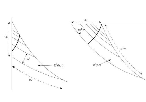
Figure 4. Singularity structure near type 3 and type 1 boundary points. An unstable curve is indicated with bold on both panels.

Recall that

(11) $$A=\cup_{H}A_{H}\text{ and }A^{\prime}=\{x_{h}\in A:\Pi_{\mathcal{D}}x_{h}\text{ is a corner point }\}$$

Let us write

(12) $$\mathcal{E}(h,n)=\mathcal{E}(x_{h},n)=\cup_{N\geq n}E^{+}(h,N),\quad\mathcal{E}_{n}=\cup_{h:x_{h}\in A^{\prime}}\mathcal{E}(h,n),$$

$$\mathcal{B}(h,n)=\mathcal{B}(x_{h},n)=\cup_{N\geq n}D^{+}(h,N),$$

(13) $$\mathcal{B}_{n}=\cup_{h:x_{h}\text{regular boundary point of a type 2 corridor}}\mathcal{B}(h,n).$$

and finally

$$\mathcal{E}_{n_{1}}\mathcal{B}_{n_{2}}=\mathcal{E}_{n_{1}}\cup\mathcal{B}_{n_{2}}$$

That is, $\mathcal{E}_{n_{1}}\mathcal{B}_{n_{2}}$ is the set of points that experience a long free flight in type 2 or type 3 corridors. This set is the disjoint union of $\mathcal{E}_{n_{1}}$ and $\mathcal{B}_{n_{2}}$, where $\mathcal{E}_{n_{1}}$ is contained in a neighborhood of $A^{\prime}$ and $\mathcal{B}_{n_{2}}$ is contained in a neighborhood of $A\setminus A^{\prime}$. Note that when there are no type 2 corridors we have $\mathcal{B}_{n_{2}}=\emptyset$. In this case, the forthcoming proof could be simplified substantially.

Let us fix a large integer $\Cl[Ns]{N:N_{0}}$ so that the sets $D^{+}(h,n)$ and $E^{+}(h^{\prime},n^{\prime})$ are disjoint whenever $n,n^{\prime}\geq\Cr{N:N_{0}}$, $h\neq h^{\prime}$. We start with a geometric lemma.

Lemma 6.

There is a constant $\Cl{c:star}$ so that for every unstable curve $W$ with $W\subset\mathcal{E}_{\Cr{N:N_{0}}}$, there is some $T=T(W)$ so that for all $x\in W$, $T\leq\tau(x)\leq\Cr{c:star}T$ holds.

Proof.

For every $h$ with $x_{h}=(r_{h},\varphi_{h})\in A^{\prime}$, we will show that the desired $\Cr{c:star}$ exists for unstable curves in $\mathcal{E}(x_{h},{\Cr{N:N_{0}}})$. This is sufficient as there are finitely many corridors and we can take the biggest $\Cr{c:star}$. Let us assume that $r_{h}$ is the left endpoint of the corresponding boundary curve $\Gamma$ (the other case is similar).

Without loss of generality we can assume that the endpoint of $W$ is a point $(r_{h},\varphi_{0})$. Indeed, if the curve does not stretch all the way to the left boundary of $\mathcal{M}$, we can smoothly extend it to the ”southwest”. A key observation is that $\varphi_{0}<\varphi_{h}$. Indeed, if $\varphi_{0}\geq\varphi_{h}$, then since unstable curves are in the ”northeast direction”, $W$ could not intersect $\mathcal{E}_{\Cr{N:N_{0}}}$. Now we choose $T=T(W)=\tau(r_{h},\varphi_{0})$. We can assume that the other edpoint of $W$ is $(r^{\prime},\varphi^{\prime})\in\partial\mathcal{E}_{\Cr{N:N_{0}}}$ so that the next collision after leaving $(r^{\prime},\varphi^{\prime})$ is at the same corner point (and so is improper). Strictly speaking, $(r^{\prime},\varphi^{\prime})$ is not contained in $W$ as $(r^{\prime},\varphi^{\prime})\notin\mathcal{E}_{\Cr{N:N_{0}}}$, that is, $W$ is a curve that does not contain one of its endpoints. Indeed, if $W$ does not fully cross $\mathcal{E}_{\Cr{N:N_{0}}}$, we can extend it smoothly to the northeast. By transverality, the triangle with vertices $(r_{h},\varphi_{h})$, $(r_{h},\varphi_{0})$ and $(r^{\prime},\varphi^{\prime})$ has angles that are bounded away from zero (specifically by an angle $\gamma$ as discussed in Section 2.3). Consequently, the distance between $(r_{h},\varphi_{h})$, and $(r^{\prime},\varphi^{\prime})$ is bounded below by a universal constant times $\varphi_{h}-\varphi_{0}$. We also know that $\varphi_{h}-\varphi_{0}\approx 1/T$, whence $\tau(r^{\prime},\varphi^{\prime})<\Cr{c:star}T$ for a geometric constant $\Cr{c:star}$. The lemma follows. ∎

Figure 4 shows unstable curves (indicated with bold) with long flight in corridors of type 1 and 3. In case of type 1 corridors, the free flight function restricted to an ustable curve $W$ may be unbounded (see the right side of figure), but any long flight is necessarily followed by a nearly grazing collision. This nearly grazing collision makes it easier to control the sum of expansion factors, as in the proof of Theorem 2. As seen on the left side of the figure and proven by Lemma 6, for any unstable curve $W$, the free flight function restricted to $W$ is bounded in type 3 corridors (with a bound depending on $W$). We will leverage this fact in Lemma 7 to show that such a flight can only increases the $\mathcal{Z}_{1}$ function of a standard family by a bounded factor.

Most work is required in case of type 2 corridors. In this case, given an unstable curve near the regular boundary point (as on the right panel of Figure 4) the free flight is unbounded and after the collision, the expansion is not large. In particular, the sum in (10) is infinite. To overcome this difficulty, we prove in Lemma 8 that the $\mathcal{Z}_{q}$ function remains finite for any $q<1$. Then, we show that multiple visits into corridors of type 2 or 3 in a short succession are not possible (Lemma 9).

Lemma 7.

There is some integer $\Cl[Ns]{n:type3}\geq\Cr{N:N_{0}}$ and a constant $\Cl{C:type3factor}$ so that for every standard pair $\ell=(W,\rho)$ with $W\subset\mathcal{E}_{\Cr{n:type3}}$,

(14) $$\mathcal{Z}_{1}(F_{*}(\ell))\leq\Cr{C:type3factor}\mathcal{Z}_{1}(\ell).$$

Proof.

Let $x_{h}=(r_{h},\varphi_{h})$ and $\ell=(W,\rho)$ be such that $W\subset\mathcal{E}(x_{h},\Cr{n:type3})$ for some $\Cr{n:type3}$ to be specified later. Assume first that $x_{h}$ is a type 3 boundary point. Let us write $V_{n}=W\cap E^{+}({x_{h},n})$ and $W_{n}=F(V_{n})$ for $n\geq\Cr{n:type3}$. Next we claim that there is a constant $\beta>0$ only depending on $\mathcal{D}$ such that for all $(r,\varphi)\in W$ and with the notation $F(r,\varphi)=(r^{\prime},\varphi^{\prime})$, we have $\cos\varphi^{\prime}\geq\beta$. Indeed, let $\beta=\alpha/2$, where $\alpha$ is the minimal angle between the half tangents of the boundary points bounding the corridors and the directions of the corresponding corridor $v_{H}$ ($\alpha>0$ by assumption (A2)). Then by choosing $\Cr{n:type3}$ sufficiently large, we can guarantee that the angle between the line segment emanating from $(r,\varphi)$ and $v_{H}$ is less than $\alpha/2$, which implies the claim. Without loss of generality we can assume that $k_{0}>\beta^{-1}$ and so for all $n\geq\Cr{n:type3}$, $W_{n}$ is a homogeneous unstable curve and the expansion of $F$ on $V_{n}$ is $\approx n$. Furthermore, a simple geometric argument shows $|W_{n}|\approx n^{-1}$ whence $|V_{n}|\approx n^{-2}$. By Lemma 6, there is some $n_{W}$ so that $F(W)=\cup_{n=n_{W}}^{\Cr{c:star}n_{W}}W_{n}$. We conclude

(15) $$\mathcal{L}_{1}(W)=\sum_{n=n_{W}}^{\Cr{c:star}n_{W}}\frac{1}{\Lambda_{n,1}}\leq C\sum_{n=n_{W}}^{\Cr{c:star}n_{W}}\frac{1}{n}\leq 2C\ln\Cr{c:star}.$$

We obtained the variant of (14), where $\rho$ is constant. Generalizing it to all admissible densities $\rho$ is standard only using (5) and (6) and so we omit the proof (see e.g. [10]).

In case $x_{h}$ is a type 2 boundary corner point, we write $V_{n}=W\cap E^{+}({x_{h},n})$ and $W_{n}=F(V_{n})$ as before. Now $W_{n}$ is not a homogeneous curve as it is further cut into infinitely many pieces by secondary singularities. However, on any of these pieces, the expansion factor is large and so $\mathcal{L}_{1}(W)$ is bounded as in [9, Remark 5.59]. The lemma follows. ∎

Lemma 8.

There is some integer $\Cl[Ns]{n:type2}\geq\Cr{n:type3}$ so that for every $q<1$ there is a constant $\Cl{C:type2factor}$ so that for every standard pair $\ell=(W,\rho)$ with $W\subset\mathcal{B}_{\Cr{n:type2}}$,

$$\mathcal{Z}_{q}(F_{*}\ell)\leq\Cr{C:type2factor}\mathcal{Z}_{q}(\ell).$$

Proof.

Let $x_{h}=(r_{h},\pm\pi/2)$ be a regular boundary point of a type 2 corridor and let $\ell=(W,\rho)$ be such that $W\subset\mathcal{B}(x_{h},\Cr{n:type2})$ for some $\Cr{n:type2}$ to be specified later. As in the case of type 3 corridors (cf. the proof of Lemma 7), we find that $V_{n}=W\cap D^{+}_{h,n}$, $W_{n}=F(V_{n})$, the expansion of $F$ on $V_{n}$ is $\approx n$, $|W_{n}|\approx n^{-1}$, and $|V_{n}|\approx n^{-2}$. The main difference from the case of type 3 corridors is that now Lemma 6 fails to hold. Indeed, the curve $W$ may be cut into infinitely many pieces (see the right panel of Figure 4) and so the sum in (15) diverges. We are going to prove that

(16) $$\sum_{n\geq\Cr{n:type2}}\left(\frac{|W|}{|W_{n}|}\right)^{q}\frac{|V_{n}|}{|W|}\leq\Cr{C:type2factor}.$$

First note that (16) implies the lemma when $\rho$ is constant. The general case can be proven using (5) and (6). Thus it remains to verify (16). To prove (16), we distinguish three cases.

First assume that $W$ is cut into infinitely many pieces, that is, $V_{n}\neq\emptyset$ for infinitely many $n$’s. Then $x_{h}$ is necessarily an endpoint of $W$. Let $M$ be the smallest integer $n$ so that $W$ fully crosses $D^{+}_{h,n}$. Then we have $|W|\approx M^{-1}$ and so

$$\sum_{n\geq\Cr{n:type2}}\left(\frac{|W|}{|W_{n}|}\right)^{q}\frac{|V_{n}|}{|W|}\leq C|W|^{q-1}\sum_{n\geq M-1}n^{-2+q}\leq C|W|^{q-1}\sum_{n\geq\bar{C}|W|^{-1}}n^{-2+q}\leq\Cr{C:type2factor}.$$

Next, assume that $W\subset D^{+}_{h,M}$ for some $M$. Then the left hand side of (16) is $(|W|/|W_{M}|)^{q}\approx M^{-q}$, which is also bounded.

Finally, assume that there are positive integers $M_{1}\leq M_{2}$ so that $V_{n}\neq\emptyset$ if and only if $M_{1}\leq n\leq M_{2}$. The contribution of $n=M_{1}$ and $n=M_{2}$ is bounded as in the second case. Thus it suffices to bound the contribution of $n=M_{1}+1,...,M_{2}-1$, that is the set of $n$’s so that $W$ fully crosses $D^{+}_{h,n}$. To simplify the notation, we replace $M_{1}+1$ by $M_{1}$ and $M_{2}-1$ by $M_{2}$. We obtain

$$\sum_{n=M_{1}}^{M_{2}}\left(\frac{|W|}{|W_{n}|}\right)^{q}\frac{|V_{n}|}{|W|}\leq C|W|^{q-1}\sum_{n=M_{1}}^{M_{2}}n^{-2+q}\leq C(M_{1}^{-1}-M_{2}^{-1})^{q-1}(M_{1}^{q-1}-M_{2}^{q-1}).$$

Writing $a=M_{2}/M_{1}-1$, we find that the above display is bounded by

$$C(M_{2}^{-1}a)^{q-1}M_{2}^{q-1}\left[\left(\frac{M_{1}}{M_{2}}\right)^{q-1}-1\right]=Ca^{q-1}[(1+a)^{1-q}-1]=:Cf(a).$$

Now $f$ is a continuous function on $\mathbb{R}_{+}$ with $\lim_{a\rightarrow\infty}f(a)=1$ and $\lim_{a\rightarrow 0}f(a)=0$ (in fact $f(a)\sim(1-q)a^{q}$ as $a\rightarrow 0$). Consequently, $f$ is bounded and so (16) follows. ∎

Remark 8.

The proof of Theorem 3 could be simplified if we knew that the constant $\Cr{C:type2factor}$ given by Lemma 8 is less than $1$. Although the 1-step expansion as required by (H5) of [10] would not follow, as it does not even hold in type C billiards, at least long flights in a short succession would not cause a trouble. Unfortunately we do not know whether $\Cr{C:type2factor}<1$ and so we need Lemma 9, which says that two long free flights in short succession emanating near a corner point are not possible.

Lemma 9.

For every $K\in\mathbb{N}$ there exists $\Cl[Ns]{N:N(K)type3}=\Cr{N:N(K)type3}(K)$ so that for all $k=1,...,K$,

$$\mathcal{E}_{\Cr{N:N(K)type3}}\cap F^{-k}(\mathcal{E}_{\Cr{N:N(K)type3}})=\emptyset.$$

The proof of Lemma 9 is longer than the proof of the other lemmas. To avoid disruption in the main ideas here, we postpone this proof to the next section.

Note that in the case of type 2 corridors, two long flights are possible. Specifically, we have

Lemma 10.

For every $K\in\mathbb{N}$ there exists $\Cl[Ns]{N:N(K)type2}=\Cr{N:N(K)type2}(K)$ so that for all $k=1,2,...,K$

$$\mathcal{B}_{\Cr{N:N(K)type2}}\cap F^{-k}(\mathcal{E}_{\Cr{N:N(K)type3}(K)}\mathcal{B}_{\Cr{N:N(K)type2}})=\emptyset$$

and for all $x\in\mathcal{E}(x_{h},{\Cr{N:N(K)type3}(K)})$, the set

$$\mathfrak{k}=\{k=1,...,K:F^{k}(x)\in\mathcal{B}_{\Cr{N:N(K)type2}}\}$$

can only be non empty if $x_{h}$ is of type 2. In this case, $\mathfrak{k}=\{1\}$ or $\mathfrak{k}=\{2\}$.

Proof.

Let

$$\Cr{N:N(K)type2}(K)=\frac{\max_{x\in A}\tau(x)}{\min_{x\in A}\tau(x)}\Cr{c:conseclongflight}\Cr{N:N(K)type3}^{2}(K+2),$$

where $\Cr{c:conseclongflight}$ is defined in Lemma 2. If $x\in\mathcal{B}(x_{h},\Cr{N:N(K)type2})$, then as in Lemma 2, we have either $F^{-1}(x)\in\mathcal{E}_{\Cr{N:N(K)type3}(K+2)}$ or $F^{-2}(x)\in\mathcal{E}_{\Cr{N:N(K)type3}(K+2)}$. Now the result follows from Lemma 9.

∎

For the remaining part of the proof let us fix some $q<1$. Recalling (6), there exists a constant $\bar{c}$ only depending on $\mathcal{D}$ so that for any standard pair $\ell=(W,\rho)$,

(17) $$1/\bar{c}\leq\mathcal{Z}_{q}(\ell)|W|^{q}\leq\bar{c},\quad 1/\bar{c}\leq\mathcal{Z}_{1}(\ell)|W|\leq\bar{c}.$$

For a given homogeneous unstable curve $W$ we write

$$\bm{T}_{N,N^{\prime}}(W)=\bm{T}_{N,N^{\prime},\mathcal{D}}(W)=\min\{m\geq 0:F^{-m}(W)\subset\mathcal{E}_{N}\mathcal{B}_{N^{\prime}}\}.$$

The next lemma states a weaker version of Theorem 3, namely, when only those H-components in $F^{m}(\ell)$ that have not visited $\mathcal{E}_{N}\mathcal{B}_{N^{\prime}}$ for some $N,N^{\prime}$ large are considered.

Lemma 11.

There exists $m_{0}\in\mathbb{N}$, and $\Cl{c:outtacorr}$ so that for every $N,N^{\prime}$ and for every $K$ there is some $\delta_{0}=\delta_{0}(N,N^{\prime},K)$ such that the following holds for every standard pair $\ell=(W,\rho)$ with $|W|<\delta_{0}$ and for all $m=1,2,...,2Km_{0}+6$

(18) $$\mathcal{Z}_{1}(F^{m}_{*}(\ell)|_{W_{i}:\bm{T}_{N,N^{\prime}}(W_{i})>m})<\Cr{c:outtacorr}\mathcal{Z}_{1}(\ell),$$

(19) $$\mathcal{Z}_{1}(F^{Km_{0}}_{*}(\ell)|_{W_{i}:\bm{T}_{N,N^{\prime}}(W_{i})>Km_{0}})<2^{-K}\mathcal{Z}_{1}(\ell).$$

Proof.

First, assume that $\rho$ is constant. Now we claim the following: there is some $m_{0}$ and $\Cr{c:outtacorr}$ so that for any $N,N^{\prime}$

(20) $$\lim_{\delta\rightarrow 0}\sup_{W:|W|<\delta}\sum_{W_{i}\in F^{m_{0}}(W):\bm{T}_{N,N^{\prime}}(W_{i})>m_{0}}\frac{1}{\Lambda_{i,m_{0}}}<\frac{1}{2},$$

and for any $m$,

(21) $$\lim_{\delta\rightarrow 0}\sup_{W:|W|<\delta}\sum_{W_{i}\in F^{m}:\bm{T}_{N,N^{\prime}}(W_{i})>m}\frac{1}{\Lambda_{i,m}}<\Cr{c:outtacorr}.$$

To prove this claim, let us replace a small neighborhood (of diameter $<cN^{-1}$) of the corner points bounding the corridors by a smooth curve so as the new billiard table $\mathcal{D}^{\prime}=\mathcal{D}^{\prime}(N)$ contains $\mathcal{D}$. By construction, for all $W_{i}$ H-component of $F_{\mathcal{D}^{\prime}}^{m}(W)$ with $\bm{T}_{N,N^{\prime},\mathcal{D}^{\prime}}(W_{i})>m$ and for all $x\in W_{i}$, the orbits $F_{\mathcal{D}}^{-m}(x),....,F_{\mathcal{D}}^{-1}(x),x$ and $F_{\mathcal{D}^{\prime}}^{-m}(x),....,F_{\mathcal{D}^{\prime}}^{-1}(x),x$ coincide. Then Theorem 2 implies that the left hand side of (20) is bounded by some number $\beta<1$. Replacing $m_{0}$ by $m_{0}^{\ln(1/2)/\ln\beta}$ and using (9) and Lemma 1, we obtain (20). Although we only proved Lemma 1 under the conditions of Theorem 2, it is valid under the more general conditions of Theorem 3. Indeed, a long flight and an almost grazing collision expands an unstable curve more than just a long flight. Likewise, we obtain

(22) $$\lim_{\delta\rightarrow 0}\sup_{W:|W|<\delta}\sum_{W_{i}\in F^{Km_{0}}:\bm{T}_{N,N^{\prime}}(W_{i})>Km_{0}}\frac{1}{\Lambda_{i,Km_{0}}}<2^{-K}.$$

Also observe that (21) follows from the proof of Theorem 2 for $m\leq m_{0}$. Then it also follows for $m\geq m_{0}$ by (20) and by (9).

Since our construction did not depend on $N^{\prime}$, it remains to prove that $m_{0}$ and $\Cr{c:outtacorr}$ are uniform in $N$. Although the curvature of $\partial\mathcal{D}^{\prime}$ is not uniformly bounded in $N$, points visiting the part of the phase space with unbounded curvature are discarded. Then it remains to observe that the constants $\Xi$ and $C_{\#}$ appearing in the proof of Theorem 2 are uniform in $\mathcal{D}^{\prime}$ and so is $m_{0}$ and $\Cr{c:outtacorr}$.

Now (22) and (21) combined with (5) and (6) imply (18) and (19).

Finally, if $\rho$ is not constant, we just need to apply (5) once more to complete the proof. ∎

In the setup of Lemma 11, we discard the points one step before reaching $\mathcal{E}_{N}\mathcal{B}_{N^{\prime}}$. The next lemma says that we can iterate the map once more and only discard the points upon reaching $\mathcal{E}_{N}\mathcal{B}_{N^{\prime}}$. Let

$$\bm{T}^{\prime}_{N,N^{\prime}}(W)=\min\{m\geq 1:F^{-m}(W)\subset\mathcal{E}_{N}\mathcal{B}_{N^{\prime}}\}.$$

Lemma 12.

There exists $\Cl{c:intocorr}$ so that for every $K$ and for every large $N,N^{\prime}$, there is some $\delta^{\prime}_{0}=\delta^{\prime}_{0}(N,N^{\prime},K)$ such that the following holds for every standard pair $\ell=(W,\rho)$ with $|W|<\delta^{\prime}_{0}$ and for all $m=1,2,...,2Km_{0}+6$

(23) $$\mathcal{Z}_{1}(F^{m}_{*}(\ell)|_{W_{i}:\bm{T}^{\prime}_{N,N^{\prime}}(W_{i})>m})<\Cr{c:intocorr}\mathcal{Z}_{1}(\ell)$$

(24) $$\mathcal{Z}_{1}(F^{Km_{0}+m}_{*}(\ell)|_{W_{i}:\bm{T}^{\prime}_{N,N^{\prime}}(W_{i})>Km_{0}+m})<\Cr{c:intocorr}2^{-K}\mathcal{Z}_{1}(\ell)$$

Proof.

First we claim that

(25) $$\mathcal{Z}_{1}(F^{Km_{0}+m}_{*}(\ell)|_{W_{i}:\bm{T}_{N,N^{\prime}}(W_{i})>Km_{0}+m})<\Cr{c:outtacorr}2^{-K}\mathcal{Z}_{1}(\ell)$$

for all standard pairs $\ell=(W,\rho)$ with $|W|<(\delta_{0})^{3^{Km_{0}}}$. Indeed, by Lemma 1, any H-component $W_{i}\subset F^{Km_{0}}(W)$ satisfies $|W_{i}|<\delta_{0}$. By applying (18) to the H-components $W_{i}\subset F^{Km_{0}}(W)$, (18) and (19) imply (25).

To derive (23), we write

$$\mathcal{Z}_{1}(F^{m}_{*}(\ell)|_{W_{i}:\bm{T}^{\prime}_{N,N^{\prime}}(W_{i})>m})$$

$$=\mathcal{Z}_{1}(F^{m}_{*}(\ell)|_{W_{i}:\bm{T}_{N,N^{\prime}}(W_{i})>m})+\mathcal{Z}_{1}(F^{m}_{*}(\ell)|_{W_{i}:W_{i}\subset\mathcal{E}_{N}\mathcal{B}_{N^{\prime}},\bm{T}_{N,N^{\prime}}(W_{i})>m})=:Z_{11}+Z_{12}$$

By (18), $Z_{11}\leq\Cr{c:outtacorr}\mathcal{Z}_{1}(\ell)$. Let us write $j\in\mathcal{J}$ if the H-component $W_{j,m-1}\subset F^{m-1}(W)$ contains a point $x\in W_{j,m-1}$ with $F(x)\in\mathcal{E}_{N}\mathcal{B}_{N^{\prime}}$ and $\bm{T}_{N,N^{\prime}}(W_{j})>m-1$. Also write $\ell_{j}=(W_{j},\rho_{j,m-1})$. Choosing $\delta^{\prime}_{0}\leq(\tilde{\delta})^{3^{2(Km_{0}+1)}}$ for some $\tilde{\delta}\leq\delta_{0}$, we have $|W_{j}|\leq\tilde{\delta}$.

We claim that there is some $\tilde{\delta}<\delta_{0}$ and $\Cl{c:TtoT^{\prime}}$ so that

(26) $$\mathcal{Z}_{1}(F_{*}(\ell_{j}))\leq\Cr{c:TtoT^{\prime}}\mathcal{Z}_{1}(\ell_{j})\text{ for all }j\in\mathcal{J}.$$

To prove (26), we first claim that there is a constant $C$ only depending on $\mathcal{D}$ so that for any $N>\Cr{N:N(K)type3}(1)$ and $N^{\prime}>\Cr{N:N(K)type2}(1)$ fixed, and for any $x\in\ell_{j}$, $\tau(x)<C$. Indeed, it is not possible for $x$ to have a long flight in a type 2 or type 3 corridor since $x\notin\mathcal{E}_{N}\mathcal{B}_{N^{\prime}}$. Let $x$ be so that $F(x)\in\mathcal{E}_{N}\mathcal{B}_{N^{\prime}}$. Then it is also not possible for $x$ to have a long flight in a type 1 corridor, because in this case $F(x)$ would be close to a boundary point of a type 1 corridor and we could not have $F(x)\in\mathcal{E}_{N}\mathcal{B}_{N^{\prime}}$. Thus $\tau(x)<C$. This estimate can be extended to all $x\in\ell_{j}$ by choosing $\tilde{\delta}<\delta_{0}$ (for example, smaller than half of the smallest distance between two distinct points in $A=\cup_{corridors}A_{H}$). Now since the free flight function on $\ell_{j}$ is uniformly bounded, (26) follows from [11].

We conclude

$$Z_{12}\leq\sum_{j\in\mathcal{J}}c_{j}\mathcal{Z}_{1}(F_{*}(\ell_{j}))\leq\Cr{c:TtoT^{\prime}}\sum_{j\in\mathcal{J}}c_{j}\mathcal{Z}_{1}(\ell_{j})$$

$$\leq\Cr{c:TtoT^{\prime}}\mathcal{Z}_{1}(F^{m-1}_{*}(\ell)|_{W_{j}:\bm{T}_{N,N^{\prime}}(W_{j})>m-1})\leq\Cr{c:TtoT^{\prime}}\Cr{c:outtacorr}\mathcal{Z}_{1}(\ell).$$

Thus (23) follows with $\Cr{c:intocorr}=\Cr{c:outtacorr}(1+\Cr{c:TtoT^{\prime}})$. The derivation of (24) from (25) is similar.

∎

Recall that two long flights are possible in a type 2 corridor, right after one another or separated by exactly one short flight. Our next lemma says that the $\mathcal{Z}_{q}$ function can be controlled throughout the course of these two long flights.

Lemma 13.

There is some $\Cl{c:threesteps}$ so that for any standard pair $\tilde{\ell}=(\tilde{W},\tilde{\rho})$ with $\tilde{W}\subset\mathcal{E}_{\Cr{N:N(K)type3}(4)}\mathcal{B}_{\Cr{N:N(K)type2}(4)}$,

$$\mathcal{Z}_{q}(F^{3}_{*}(\tilde{\ell}))\leq\Cr{c:threesteps}\mathcal{Z}_{q}(\tilde{\ell}).$$

We finish the proof of the theorem first and then will prove Lemma 13. First, we fix a large constant $K$ so that

(27) $$\Cr{c:intocorr}\bar{c}^{4}2^{-qK}(1+(2Km_{0})\Cr{c:threesteps}\Cr{c:intocorr}\bar{c}^{4})<\frac{1}{2}$$

holds. Next, we choose $M=2Km_{0}+6$. Then, we choose $\tilde{N}=\Cr{N:N(K)type3}(M)$, $\tilde{N}^{\prime}=\Cr{N:N(K)type2}(M)$. Note that by Lemma 10, for every $x\in\mathcal{M}$ there exists $m=0,...,M$ so that

(28) $$\{x,F(x),...,F^{M}(x)\}\cap\mathcal{E}_{\tilde{N}}\mathcal{B}_{\tilde{N}^{\prime}}\subset\{m,m+1,m+2\}.$$

Finally, we fix $\delta^{\prime}_{0}=\delta^{\prime}_{0}(\tilde{N},\tilde{N}^{\prime},K)$ as given by Lemma 12. Then we choose $\delta_{1}$ so small that for any $W$ with $|W|<\delta_{1}$, for any $m=1,...,M$, any H-component of $F^{m}(W)$ is shorter than $\delta^{\prime}_{0}$ (e.g., $\delta_{1}=(\delta^{\prime}_{0})^{3^{M}}$ works by Lemma 1).

We are going to prove Theorem 3 with $\varkappa=1/2$, $\delta=\delta_{1}$ and $M$ as chosen above.

Note that all standard pairs in the proof are shorter than $\delta_{0}^{\prime}$. Thus, by further reducing $\delta_{0}^{\prime}$ if necessary, we can assume that any standard pair intersecting $\mathcal{E}_{\tilde{N}}\mathcal{B}_{\tilde{N}^{\prime}}$ is fully contained in $\mathcal{E}_{\tilde{N}-1}\mathcal{B}_{\tilde{N}^{\prime}-1}$. To simplify notations, we will assume that once a standard pair intersects $\mathcal{E}_{\tilde{N}}\mathcal{B}_{\tilde{N}^{\prime}}$, it is also fully contained in $\mathcal{E}_{\tilde{N}}\mathcal{B}_{\tilde{N}^{\prime}}$.

Let us fix a standard pair $\ell=(W,\rho)$ with $|W|<\delta_{1}$, let $W_{i,m}$ denote an H-component of $F^{m}(W)$ and write $F^{M}_{*}(\ell)=\sum_{i}c_{i,M}\ell_{i}$, where $\ell_{i}=(W_{i,M},\rho_{i,M})$. The idea of the proof is now the following. Let the time of the first visit to $\mathcal{E}_{\tilde{N}}\mathcal{B}_{\tilde{N}^{\prime}}$ be $m$. Then no visit to $\mathcal{E}_{\tilde{N}}\mathcal{B}_{\tilde{N}^{\prime}}$ is possible any time after $m+2$ by Lemma 10. If $m\leq M/2$, then $M-m-3>Km_{0}$ and so we can use (24) after the last visit to show that the $Z$ function does not grow. Likewise, if $m>M/2$, we will use (24) at time zero (before the visit).

To make this idea precise, for all standard pairs $\ell_{i,M}$ we associate a set $\mathcal{T}_{i}$ of integers so that for any $x\in F^{-M}(W_{i,M})$, we have $F^{k}(x)\in\mathcal{E}_{\tilde{N}}\mathcal{B}_{\tilde{N}^{\prime}}$ for $k=0,1,...,M-1$ if and only if $k\in\mathcal{T}_{i}$. By Lemma 10, all associated sets $\mathcal{T}$ can contain up to 2 integers. Furthermore, if $\mathcal{T}$ contains exactly 2 numbers, then $\mathcal{T}=\{m,m+1\}$ or $\mathcal{T}=\{m,m+2\}$ for some $m=0,...,M-1$. We have $\mathcal{Z}_{q}(F^{M}_{*}(\ell))=\sum_{i}c_{i,M}\mathcal{Z}_{q}(\ell_{i,M})$. Now let

$$Z_{m}=\mathcal{Z}_{q}(F^{M}_{*}(\ell)|_{W_{i}:\min\mathcal{T}_{i}=m})$$

and

$$Z_{M+}=\mathcal{Z}_{q}(F^{M}_{*}(\ell)|_{W_{i}:\mathcal{T}_{i}=\emptyset})=\mathcal{Z}_{q}(F^{M}_{*}(\ell)|_{W_{i}:\bm{T}^{\prime}_{\tilde{N},\tilde{N}^{\prime}}(W_{i})>M}).$$

Clearly, we have

(29) $$\mathcal{Z}_{q}(F^{M}_{*}(\ell))=\left[\sum_{m=0}^{M-1}Z_{m}\right]+Z_{M+}.$$

Given a substandard family $\mathcal{G}=(\ell_{\alpha}=(W_{\alpha},\rho_{\alpha})_{\alpha\in\mathbb{N}},\lambda)$ ( recall that substandard means $s=\sum_{\alpha=1}^{\infty}\lambda_{\alpha}\leq 1$), we have

$$\mathcal{Z}_{q}(\mathcal{G})=\sum_{\alpha=1}^{\infty}\lambda_{\alpha}\mathcal{Z}_{q}(\ell_{\alpha}) \leq\bar{c}s\sum_{\alpha=1}^{\infty}\frac{\lambda_{\alpha}}{s}\frac{1}{|W_{\alpha}|^{q}}$$

$$\leq\bar{c}s\left[\sum_{\alpha=1}^{\infty}\frac{\lambda_{\alpha}}{s}\frac{1}{|W_{\alpha}|}\right]^{q}\leq\bar{c}^{2}s^{1-q}[\mathcal{Z}_{1}(\mathcal{G})]^{q}$$

(30) $$\leq\bar{c}^{2}[\mathcal{Z}_{1}(\mathcal{G})]^{q},$$

where we used (17) in the first two lines and Jensen’s inequality in the second line. Now combining (24) with (30), we find

(31) $$Z_{M+}\leq\bar{c}^{2}[\Cr{c:intocorr}2^{-K}\mathcal{Z}_{1}(\ell)]^{q}\leq\bar{c}^{2}\left[\Cr{c:intocorr}2^{-K}\bar{c}\frac{1}{|W|}\right]^{q}\leq\Cr{c:intocorr}\bar{c}^{4}2^{-qK}\mathcal{Z}_{q}(\ell).$$

Next, fix some $m\in[0,M/2]$ and consider the substandard family

$$\mathcal{G}_{m}=(\ell_{i,m}=(W_{i,m},\rho_{i,m})_{i\in\mathcal{I}_{m}},\lambda_{i}=c_{i,m}),$$

where $i\in\mathcal{I}_{m}$ if

$$W_{i,m}\in\mathcal{E}_{\tilde{N}}\mathcal{B}_{\tilde{N}^{\prime}},\bm{T}^{\prime}_{\tilde{N},\tilde{N}^{\prime}}(W_{i,m})>m.$$

Note that $\mathcal{G}_{m}$ corresponds to the image under $F^{m}$ of the points in $W$ whose first hitting time of the set $\mathcal{E}_{\tilde{N}}\mathcal{B}_{\tilde{N}^{\prime}}$ is exactly $m$ and so

$$Z_{m}=\mathcal{Z}_{q}(F_{*}^{M-m}(\mathcal{G}_{m})).$$

By (23),

$$\mathcal{Z}_{1}(\mathcal{G}_{M-m})\leq\Cr{c:intocorr}\mathcal{Z}_{1}(\ell).$$

Now using (30) we compute as in (31) that

(32) $$\mathcal{Z}_{q}(\mathcal{G}_{m})\leq\bar{c}^{2}[\mathcal{Z}_{1}(\mathcal{G}_{m})]^{q}\leq\bar{c}^{2}[\Cr{c:intocorr}\mathcal{Z}_{1}(\ell)]^{q}\leq\Cr{c:intocorr}\bar{c}^{4}\mathcal{Z}_{q}(\ell).$$

Now fix some $\ell_{i,m}=(W_{i,m},\rho_{i,m})\in\mathcal{G}_{m}$. By Lemma 13, we have

(33) $$\mathcal{Z}_{q}(F^{3}_{*}(\ell_{i,m}))\leq\Cr{c:threesteps}\mathcal{Z}_{q}(\ell_{i,m}).$$

Now fix any $W_{j,m+3}\in F^{3}(W_{i,m})$. By (30),

$$\mathcal{Z}_{q}(F^{M-m-3}_{*}(\ell_{j,m+3}))\leq\bar{c}^{2}[\mathcal{Z}_{1}(F^{M-m-3}_{*}(\ell_{j,m+3}))]^{q}.$$

By (28), no points of $W_{j,m+3}$ can visit $\mathcal{E}_{\tilde{N}}\mathcal{B}_{\tilde{N}^{\prime}}$ for $M-m-3$ iterations. Combining this observation with the fact that $M-m-3\geq Km_{0}$ and with (24), we find

(34) $$\mathcal{Z}_{q}(F^{M-m-3}_{*}(\ell_{j,m+3}))\leq\bar{c}^{2}[\Cr{c:intocorr}2^{-K}\mathcal{Z}_{1}(\ell_{j,m+3}))]^{q}\leq\Cr{c:intocorr}\bar{c}^{4}2^{-qK}\mathcal{Z}_{q}(\ell_{j,m+3}).$$

Now combining (33) and (34) we find

$$Z_{m}=\mathcal{Z}_{q}(F^{M-m}_{*}(\mathcal{G}_{m}))\leq\Cr{c:threesteps}\Cr{c:intocorr}\bar{c}^{4}2^{-qK}\mathcal{Z}_{q}(\mathcal{G}_{m}),$$

and so by (32)

(35) $$Z_{m}\leq\Cr{c:threesteps}(\Cr{c:intocorr})^{2}\bar{c}^{8}2^{-qK}\mathcal{Z}_{q}(\ell).$$

Finally, let us consider the case $m\in[M/2+1,M]$ and define $\mathcal{G}_{m}$ as before. Since $m>Km_{0}$, we have by (24) that

$$\mathcal{Z}_{1}(\mathcal{G}_{m})\leq\Cr{c:intocorr}2^{-K}\mathcal{Z}_{1}(\ell),$$

and so by (30),

$$\mathcal{Z}_{q}(\mathcal{G}_{m})\leq\Cr{c:intocorr}2^{-qK}\bar{c}^{4}\mathcal{Z}_{q}(\ell).$$

Now Lemma 13 implies

$$\mathcal{Z}_{q}(F^{3}_{*}(\mathcal{G}_{m}))\leq\Cr{c:threesteps}\mathcal{Z}_{q}(\mathcal{G}_{M-m}).$$

Finally, for any $\ell_{j}\in F^{3}_{*}(\mathcal{G}_{m})$, we combine (30), (28) and (23) to conclude

$$\mathcal{Z}_{q}(F_{*}^{M-m-3}(\ell_{j}))\leq\bar{c}^{2}[\mathcal{Z}_{1}(F_{*}^{M-m-3}(\ell_{j}))]^{q}\leq\bar{c}^{2}[\Cr{c:intocorr}\mathcal{Z}_{1}(\ell_{j})]^{q}\leq\Cr{c:intocorr}\bar{c}^{4}\mathcal{Z}_{q}(\ell_{j}).$$

Combining the last three displayed inequalities, we obtain

(36) $$Z_{m}\leq\Cr{c:threesteps}(\Cr{c:intocorr})^{2}\bar{c}^{8}2^{-qK}\mathcal{Z}_{q}(\ell).$$

Now we substite the estimates (31), (35) and (36) into (29) to conclude

(37) $$\mathcal{Z}_{q}(F^{M}_{*}(\ell))\leq\Cr{c:intocorr}\bar{c}^{4}2^{-qK}(1+(2Km_{0})\Cr{c:threesteps}\Cr{c:intocorr}\bar{c}^{4})\mathcal{Z}_{q}(\ell).$$

The right hand side of (37) is bounded by $\mathcal{Z}_{q}(\ell)/2$ by (27). This completes the proof of Theorem 3 assuming Lemma 13. In the remaining part of this section, we give a proof of this lemma.

Proof of Lemma 13.

Let us write $\Cr{N:N(K)type2}=\Cr{N:N(K)type2}(4)$ and $\Cr{N:N(K)type3}=\Cr{N:N(K)type3}(4)$. We will distinguish three cases.

Case 1: $\tilde{W}\subset\mathcal{B}_{\Cr{N:N(K)type2}}$. By Lemma 8, we have

$$\mathcal{Z}_{q}(F_{*}(\tilde{\ell}))<\Cr{C:type2factor}\mathcal{Z}_{q}(\tilde{\ell})$$

and by Lemma 10, we have

(38) $$(F(\tilde{W})\cup F^{2}(\tilde{W}))\cap(\mathcal{E}_{\Cr{N:N(K)type3}}\mathcal{B}_{\Cr{N:N(K)type2}})=\emptyset.$$

Consequently, as in (26), for any standard pair $\tilde{\ell}^{\prime}=(\tilde{W}^{\prime},\tilde{\rho}^{\prime})$ in the standard family $F_{*}(\tilde{\ell})$, we have

(39) $$\mathcal{Z}_{1}(F^{2}_{*}(\tilde{\ell}^{\prime}))\leq\Cr{c:TtoT^{\prime}}^{2}\mathcal{Z}_{1}(\tilde{\ell}^{\prime}).$$

Using (30), we conclude

$$\mathcal{Z}_{q}(F^{3}_{*}(\tilde{\ell}))\leq\bar{c}^{4}\Cr{C:type2factor}\Cr{c:TtoT^{\prime}}^{2}\mathcal{Z}_{q}(\tilde{\ell}).$$

Case 2: $\tilde{W}\subset\mathcal{E}(x_{h},\Cr{N:N(K)type3})$ for some type 3 boundary point $x_{h}$. By Lemma 7, we have

(40) $$\mathcal{Z}_{1}(F_{*}(\tilde{\ell}))\leq\Cr{C:type3factor}\mathcal{Z}_{1}(\tilde{\ell}).$$

As in case 1, (38) and (39) hold. Thus $\mathcal{Z}_{1}(F^{3}_{*}(\tilde{\ell}))\leq\Cr{c:TtoT^{\prime}}^{2}\Cr{C:type3factor}\mathcal{Z}_{1}(\tilde{\ell})$ and so

$$\mathcal{Z}_{q}(F^{3}_{*}(\tilde{\ell}))\leq\bar{c}^{4}\Cr{c:TtoT^{\prime}}^{2}\Cr{C:type3factor}\mathcal{Z}_{q}(\tilde{\ell}).$$

Case 3: $\tilde{W}\subset\mathcal{E}(x_{h},\Cr{N:N(K)type3})$ for some type 2 boundary point $x_{h}$. As in case 2, (40) holds. By Lemma 2 and by the choice of ${\Cr{N:N(K)type2}}$, we can write

$$F(\tilde{W})=\left(\cup_{i\in I_{1}}\tilde{W}_{i}\right)\cup\left(\cup_{i\in I_{2}}\tilde{W}_{i}\right)\cup\left(\cup_{i\in I_{3}}\tilde{W}_{i}\right),$$

where $\tilde{W}_{i}\subset\mathcal{B}_{\Cr{N:N(K)type2}}$ for all $i\in I_{1}$, $F(\tilde{W}_{i})\subset\mathcal{B}_{\Cr{N:N(K)type2}}$ for all $i\in I_{2}$ and $(\tilde{W}_{i}\cup F(\tilde{W}_{i}))\cap(\mathcal{E}_{\Cr{N:N(K)type3}}\mathcal{B}_{\Cr{N:N(K)type2}})=\emptyset$ for all $i\in I_{3}$. As in case 1, we derive

$$\mathcal{Z}_{q}(F^{2}_{*}(\tilde{\ell}_{i}))<\bar{c}^{4}\Cr{C:type2factor}\Cr{c:TtoT^{\prime}}^{2}\mathcal{Z}_{q}(\tilde{\ell}_{i})$$

for all $i\in I_{1}$. For $i\in I_{2}$, we have

$$\mathcal{Z}_{1}(F_{*}(\tilde{\ell}_{i}))\leq\Cr{c:TtoT^{\prime}}\mathcal{Z}_{1}(\tilde{\ell}_{i})$$

as in (26). Next, for any $\tilde{\ell}_{i,j}\in F_{*}(\tilde{\ell}_{i})$ with $i\in I_{2}$,

$$\mathcal{Z}_{q}(F_{*}(\tilde{\ell}_{i,j}))<\Cr{C:type2factor}\mathcal{Z}_{q}(\tilde{\ell}_{i,j})$$

by Lemma 8. Finally, for $i\in I_{3}$, we have

$$\mathcal{Z}_{1}(F^{2}_{*}(\tilde{\ell}_{i}))\leq\Cr{c:TtoT^{\prime}}^{2}\mathcal{Z}_{1}(\tilde{\ell}_{i})$$

as in (26).

Combining the above estimates, we obtain

$$\mathcal{Z}_{q}(F^{3}_{*}(\tilde{\ell}))\leq\bar{c}^{6}\Cr{C:type3factor}[3\Cr{C:type2factor}\Cr{c:TtoT^{\prime}}^{2}]\mathcal{Z}_{q}(\tilde{\ell}).$$

The lemma follows with $\Cr{c:threesteps}=3\bar{c}^{6}\Cr{C:type3factor}\Cr{C:type2factor}\Cr{c:TtoT^{\prime}}^{2}$.

∎

6. Proof of Lemma 9

We can assume $\Cr{N:N(K)type3}\geq\Cr{n:type2}$. Let

$$B=\cup_{H\text{ type 3 corridors}}A_{H}.$$

First we prove the lemma under simplifying assumptions and then we proceed to more general cases. All important ideas appear in the simplest Case 1, but we need to consider several other cases to allow for the singular behavior of the orbit of $B$.

Case 1: No type 2 corridors and $B\cap R_{-\infty,-2}^{\mathbb{H}}=\emptyset$. Note that the second assumption means that for any $x\in B$ and for all $n\geq 1$, $F^{n}$ is continuous at $F^{2}(x)$ (recall that the configurational component of $F(x)$ for $x\in B$ is always a corner point by definition (3)).

Since the sets $E^{+}(h,n)$ are disjoint and $B$ is finite, we can find some $\bar{N}$ so that

(41) $$\{F^{k}(x):k=1,...,K,x\in B\}\cap\mathcal{E}_{\bar{N}}=\emptyset.$$

Assume by contradiction that for all $\Cr{N:N(K)type3}\geq\Cr{n:type2}$ there is some point $(p_{0},\psi_{0})$ so that

(42) $$(p_{0},\psi_{0})\in\mathcal{E}_{\Cr{N:N(K)type3}},(p_{i},\psi_{i})=F^{i}(p_{0},\psi_{0}):(p_{\bar{k}},\psi_{\bar{k}})\in\mathcal{E}_{\Cr{N:N(K)type3}}\text{ for some }\bar{k}=1,...,K.$$

As we will see later, $p_{i}$ is not a corner point for any $i=1,...,\bar{k}$, so the points $(p_{i},\psi_{i})$ are uniquely defined. By passing to a subsequence of positive integers $\Cr{N:N(K)type3}$, we can assume that $\bar{k}$ does not depend on $\Cr{N:N(K)type3}$.

Recall Figure 2. Without loss of generality and passing to a further subsequence, we can assume that $(p_{0},\psi_{0})$ is in a small neighborhood of $(r_{H,r,1},\varphi_{H,r,1})$ (the other 3 cases are similar). Then the free flight emanating from $(p_{0},\psi_{0})$ is almost horizontal and is in the northeast direction. Consequently, $(p_{1},\psi_{1})$ is in a small neighborhood of $(r_{H,l,2},-\varphi_{H,l,2})=F(r_{H,l,1},\varphi_{H,l,1})$ (also recall (3)). Now let $W\subset\mathcal{M}$ be the line segment between the points $(r_{H,l,2},-\varphi_{H,l,2})$ and $(p_{1},\psi_{1})$. We record for later usage that the tangent of $W$ satisfies $d\varphi/dr\geq 0$. Indeed, this follows from the convexity of $\Gamma_{2,2}$. Also note that $d\varphi/dr=\infty$ is possible as we can have $p_{1}=r_{H,l,2}$. Although $W$ may not be an unstable curve, $F^{i}(W)$ will be an unstable curve for all $i\geq 1$ by the definition of unstable cones.

By the second assumption of Case 1, we can find a small $\varepsilon$ so that $F^{K}$ is continuous on the $\varepsilon$ neighborhood of $F(r_{H,l,2},-\varphi_{H,l,2})$. Next observe that there is some $\hat{N}$ so that $F^{2}(\mathcal{E}((r_{H,r,1},\varphi_{H,r,1}),\hat{N}))$ is a subset of the $\varepsilon$ neighborhood of $F(r_{H,l,2},-\varphi_{H,l,2})$. Now we choose $\Cr{N:N(K)type3}>\max\{\bar{N},\hat{N}\}$. Since $\Cr{N:N(K)type3}>\hat{N}$, $F^{K}(W)$ is a connected homogeneous unstable curve, that is, the trajectory of $W$ avoids the singularity set $R_{0}^{\mathbb{H}}$ up to $K$ iterations. Since $(p_{\bar{k}},\psi_{\bar{k}})\in F^{\bar{k}-1}(W)\cap\mathcal{E}_{\Cr{N:N(K)type3}}$ and $F^{\bar{k}}(W)$ is homogeneous, we also have $F^{\bar{k}-1}(W)\subset\mathcal{E}_{\Cr{N:N(K)type3}}$. Thus

$$F^{\bar{k}}(r_{H,l,1},\varphi_{H,l,1})=F^{\bar{k}-1}(r_{H,l,2},-\varphi_{H,l,2})\in F^{\bar{k}-1}(W)\subset\mathcal{E}_{\Cr{N:N(K)type3}}.$$

Since $\Cr{N:N(K)type3}>\bar{N}$, this is a contradiction with the choice of $\bar{N}$.

Case 2 No type 2 corridors and for all $x\in B$, and for all $n\geq 2$, $\Pi_{\mathcal{D}}F^{n}(x)$ is a regular point. The second assumption means that the future trajectory of points in $B$, after the first collision, can contain grazing collisions but no corner points.

We use the same idea as in the proof of Case 1 with the main difference that we need to study the flow instead of the map as the latter may not be continuous at $F(r_{H,l,2},-\varphi_{H,l,2})$. To derive the contradiction, we need to consider possibly different collision times $\bar{k}$ and $\hat{k}$ of the points $(p_{0},\psi_{0})$ and $(r_{H,l,1},\varphi_{H,l,1})$.

First, we update the definition of $\bar{N}$ by replacing $k=1,...,K$ by $k=1,...,L$ in (41), where $L$ is a constant only depending on $\mathcal{D}$ and $K$ so that for any $x\in B$, the first $L$ collisions in the future contain at least $K+1$ non-grazing collisions:

(43) $$\{F^{k}(x):k=1,...,L,x\in B\}\cap\mathcal{E}_{\bar{N}}=\emptyset.$$

To prove that such an $L$ exists, observe that for a given $K$ there is a $\delta>0$ so that the orbit of $B$ up to $K$ collisions avoids the $\delta$ neighborhood of the type 1 boundary points (as all type 1 boundary points are invariant under the billiard map). Thus all free flight before the next $K$ collisions is bounded by some constant $\tau_{K}$ on $B$. Also note that two grazing collisions are necessarily separated by a time $\tau_{*}$ (this is obvious in case the collisions happen on different scatterers, and by [6], corner sequences can only contain one grazing collision). Thus we can choose $L=(K+1)\tau_{K}/\tau_{*}$.

Next we claim that there is some $\varepsilon$ so that

(44) $$dist(\cup_{k=1}^{L}F^{k}(B),\mathcal{E}_{\bar{N}})>\varepsilon.$$

To prove (44), first note that for every $x\in B$, $F^{k}(x)$ cannot be in $\mathcal{E}_{\bar{N}}$ by the definition of $\bar{N}$. Furthermore, $F^{k}(x)\notin\partial\mathcal{E}_{\bar{N}}$ for $x\in B$ because otherwise $\Pi_{\mathcal{D}}F^{k}(x)$ would be a corner point, contradicting the assumptions of Case 2. Thus the desired $\varepsilon>0$ exists.

Since the forward orbit of $F(r_{H,l,2},-\varphi_{H,l,2})$ only contains regular points, for any $t\geq 0$, the flow $\Phi^{t}$ is continuous at the point $F(r_{H,l,2},-\varphi_{H,l,2})$ (recall that $\mathcal{M}$ is identified with a subset of $\Omega$). The continuity of the flow at points whose orbit avoids corner points follows from [9, Exercise 2.27].

Let $\mathcal{T}_{k}=\sum_{\ell=0}^{k-1}\tau(F^{\ell}(r_{H,l,2},-\varphi_{H,l,2}))$. Let $\mathcal{P}$ be the configurational component of the trajectory of $F(r_{H,l,2},-\varphi_{H,l,2})$ under the flow in time $\mathcal{T}_{L}$. Let $\bar{\varepsilon}\in(0,\varepsilon)$ be so small that any trajectory of the flow up to time $\mathcal{T}_{L}$ that stays $\bar{\varepsilon}$ close to $\mathcal{P}$ can only have a collision with angle $\varphi$, $\cos(\varphi)>\bar{\varepsilon}$ whenever $\bar{\varepsilon}$ close to a non-grazing collision of $\mathcal{P}$.

Next we claim the following. There is some $\hat{N}$ large enough so that for any $\Cr{N:N(K)type3}>\hat{N}$ and for any given $(p_{0},\psi_{0})$ satisfying (42) we can find $\hat{k}\leq L$ so that $(p_{\bar{k}},\psi_{\bar{k}})$ is $\bar{\varepsilon}$ close to $F^{\hat{k}}(r_{H,l,2},-\varphi_{H,l,2})$. To prove this claim, observe that the continuity of $\Phi^{\mathcal{T}_{L}}$ at $F(r_{H,l,2},-\varphi_{H,l,2})$ implies the existence of $\hat{N}$ so that if $(p_{0},\psi_{0})\in\mathcal{E}_{\hat{N}}$, and so $(p_{2},\psi_{2})$ is close to $F(r_{H,l,2},-\varphi_{H,l,2})$, then the trajectories of these two points remain $\bar{\varepsilon}$ close up to $\mathcal{T}_{L}$ flow time. It remains to define $\hat{k}$ as the number of collisions in the orbit of $F(r_{H,l,2},-\varphi_{H,l,2})$ before flow time $\mathcal{U}+\bar{\varepsilon}$, where $\mathcal{U}=\sum_{\ell=1}^{\bar{k}-1}\tau(p_{\ell},\psi_{\ell})$. By construction, $F(r_{H,l,2},-\varphi_{H,l,2})$ experiences at most $\bar{k}$ non-grazing collisions before flow time $\mathcal{U}+\bar{\varepsilon}$ and so $\hat{k}\leq L$ holds.

We choose $\Cr{N:N(K)type3}>\max\{\bar{N},\hat{N}\}$ as before. We derived that $(p_{\bar{k}},\psi_{\bar{k}})$ is $\bar{\varepsilon}$ close to $F^{\hat{k}}(r_{H,l,2},-\varphi_{H,l,2})$. Now recall from (44) that $F^{\hat{k}}(r_{H,l,2},-\varphi_{H,l,2})$ is not in the $\varepsilon$ neighborhood of $\mathcal{E}_{\bar{N}}$. This contradicts (42).

Case 3 No type 2 corridors and for all $x\in B$, and for all $n\geq 2$, $\Pi_{\mathcal{D}}F^{n}(x)$ is not a boundary point of a corridor. The future trajectories of points in $B$, after the first collision, are now allowed to contain corner points, but they cannot return to $B$.

An important observation is that the orbit of $B$ cannot contain type 1 boundary points. Indeed, the preimage of any type 1 boundary point is itself.

Recall that now the billiard (both flow and map) can be multivalued at $F(r_{H,l,2},-\varphi_{H,l,2})$. We say that a multivalued map $T$ is multicontinuous at $x$ if for every $\varepsilon$ there is some $\delta$ so that for any $y$ with $dist(x,y)<\delta$ there is a mapping $g_{x,y}$ from $T(y)$ to $T(x)$ (recall that these are sets now!) so that for any $z\in T(y)$, $dist(z,g_{x,y}(z))<\varepsilon$. By our definition of the billiard at corner points and by the assumption of Case 3, $\Phi^{t}$ is multicontinuous at $F(r_{H,l,2},-\varphi_{H,l,2})$ for any $t\geq 0$. Indeed, the values of the flow were defined as the possible limit points of nearby regular trajectories.

Now observe that (43) is still valid. Furthermore, (44) also remains true but requires a new proof. Since the future orbit of $B$ can contain corner points, a priori it may be possible that $F^{k}(x)\cap\partial\mathcal{E}_{\bar{N}}\neq\emptyset$. However, the intersection is finite and cannot contain points in $B$ by the assumption of Case 3. Thus for any point $y\in F^{k}(x)\cap\partial\mathcal{E}_{\bar{N}}$ there is some $h$ and $N(y)$ so that $y\in\partial E^{+}(h,N(y))$. Since there are finitely many points $y$, we still can guarantee (44) by choosing $\bar{N}>\max_{y}N(y)$.

Now we can conclude the proof of the lemma as in Case 2 with the only difference that we use one element of each of the sets $F^{\hat{k}}(r_{H,l,2},-\varphi_{H,l,2})$ and $F^{\bar{k}}(p_{0},\psi_{0})$ to derive the contradiction.

Case 4 No type 2 corridors The difference from Case 3 is that now points in $B$ are allowed to return to $B$ under branches of iterates of $F$.

First, observe that (43) is still valid. Indeed, if $F^{k_{1}}(x_{1})=x_{2}$ for some $x_{1},x_{2}\in B$, then by definition $x_{2}\notin\mathcal{E}_{\Cr{N:N_{0}}}$ as $x_{2}$ does not have long free flight. In Case 4, (44) is not true as $F^{k}(B)$ may intersect with $B$, and for any positive integer $N$, $B\subset\partial\mathcal{E}_{N}$. However, we have the weaker statement

$$\mathop{\mathrm{dist}}\nolimits(\cup_{k=1}^{L}F^{k}(B)\setminus B,\mathcal{E}_{\bar{N}})<\varepsilon$$

which is proved exactly as in Case 3.

Consider one element of the set $F^{\bar{k}}(p_{0},\psi_{0})\cap\mathcal{E}_{\Cr{N:N(K)type3}}$. Denote this point by $(p_{\bar{k}},\psi_{\bar{k}})$. Once $(p_{\bar{k}},\psi_{\bar{k}})$ is fixed, we can find a unique sequences of points $(p_{k},\psi_{k})$ so that $(p_{k},\psi_{k})\in F(p_{k-1},\psi_{k-1})$ for $k=1,...,\bar{k}$. Likewise, we can find a unique sequence of points $y_{1},...,y_{k_{1}}$ so that $y_{1}=(r_{H,l,2},-\varphi_{H,l,2})$, $y_{k}\in F^{s_{k}}(y_{k-1})$ and $y_{k}$ is $\bar{\varepsilon}$ close to $(p_{k},\psi_{k})$. This is the same construction as in Case 3; the only difference is that we can only go up to iterate

$$k_{1}=\min\{k:y_{k}\in B\}\wedge\hat{k}.$$

Indeed, the construction of Case 3 works up to the first time $y_{k}\in B$. If $\hat{k}<\min\{k:y_{k}\in B\}$, then the proof is completed as in Case 3. Assume now that $\hat{k}=\min\{k:y_{k}\in B\}$. Recalling the definition of $W$ from Case 1, we see that $y_{k_{1}}$ and $(p_{k_{1}},\psi_{k_{1}})$ are on a short unstable curve. That is, the tangent of the line segment $(y_{k_{1}},(p_{k_{1}},\psi_{k_{1}}))$ satisfies $d\varphi/dr\geq 0$. But note that for any point $z\in\mathcal{E}(y_{k_{1}},\Cr{N:N(K)type3})$ the tangent of the line segment $(y_{k_{1}},z)$ satisfies $d\varphi/dr<0$ (see one case on the left panel of Figure 4. In the other case, i.e. when $\Pi_{\mathcal{D}}y_{k_{1}}$ is the right endpoint of $\Gamma_{ij}$, the region $\mathcal{E}(y_{k_{1}},\Cr{N:N(K)type3})$ is to the northwest from $y_{k_{1}}$.) This means that $(p_{k_{1}},\psi_{k_{1}})$ cannot be in $\mathcal{E}_{\Cr{N:N(K)type3}}$ which is a contradiction. Now assume that $\hat{k}>k_{1}$. Assume that $y_{k}=(r_{H,r,1},\varphi_{H,r,1})$ (the other three cases are similar). Then define $y_{k_{1}+1}=(r_{H,r,2},-\varphi_{H,r,2})$ and $(p_{k_{1}+1},\psi_{k_{1}+1})=F(p_{k_{1}},\psi_{k_{1}})$ (which exists uniquely as $\bar{\varepsilon}$ is small). Furthermore, the line segment $W_{1}$ joining $y_{k_{1}+1}$ and $(p_{k_{1}+1},\psi_{k_{1}+1})$ has a tangent that satisfies $d\varphi/dr\geq 0$. Then we can repeat the previous construction with $(p_{0},\psi_{0})$ replaced by $(p_{k_{1}+1},\psi_{k_{1}+1})$ and $y_{1}$ replaced by $y_{k_{1}+1}$. Let

$$k_{2}=\min\{k>k_{1}:y_{k}\in B\}\wedge\hat{k}.$$

If $\hat{k}\leq\min\{k>k_{1}:y_{k}\in B\}$, then the proof is completed as before. If $\hat{k}>\min\{k>k_{1}:y_{k}\in B\}$, then we can define $(p_{k_{2}+1},\psi_{k_{2}+1})$, $y_{k_{2}+1}$ as before. Following this procedure inductively, we consider as many $k_{\ell}$’s as needed. For some $\ell<K$, we will have $\hat{k}<k_{\ell}$ whence we can finish the proof.

Case 5 Some type 2 corridors

When type 2 corridors are allowed, the previous proof can be repeated with minor changes, which we list next. First, we replace $B$ by $A^{\prime}$, where $A^{\prime}$ is defined in (11). Let $(p_{0},\psi_{0})\in\mathcal{E}(x_{h},\Cr{N:N(K)type3})$ as before. If $x_{h}\in B$, we proceed as before. Assume now that $x_{h}=(r_{h},\varphi_{h})\in A^{\prime}\setminus B$. Then the boundary points of the corresponding corridor $H$ are

$$A_{H}=\{x_{h}=(r_{h},\varphi_{h}),x_{h^{\prime}}=(r_{h^{\prime}},\varphi_{h^{\prime}}),(r_{h^{\prime\prime}},-\pi/2),(r_{h^{\prime\prime}},\pi/2)\}.$$

Here, $r_{h}$ and $r_{h^{\prime}}$ correspond to the corner point on one side of the corridor, and the points $(r_{h^{\prime\prime}},\pm\pi/2)$ correspond to the regular boundary point of the corridor. As in Lemma 2, we find that either $F^{2}(p_{0},\psi_{0})$ or $F^{3}(p_{0},\psi_{0})$ is in a small neighborhood of $(r_{h^{\prime}},-\varphi_{h^{\prime}})$. Indeed, the particle starting from $(p_{0},\psi_{0})$ experiences a long free flight, after which it collides once or twice in a small neighborhood of the regular boundary point of the corridor, and then has another long free flight terminating in a small neighborhood of the boundary corner point. Replacing $(p_{1},\psi_{1})$ with either $F^{2}(p_{0},\psi_{0})$ or $F^{3}(p_{0},\psi_{0})$ (whichever is close to $(r_{h^{\prime}},-\varphi_{h^{\prime}})$), and making similar adjustment at all times $k_{1},k_{2},...,k_{\ell}$ as introduced in Case 4, we can repeat the proof of Case 4.

7. Proof of Theorem 4

Theorem 4 is quite intuitive. Indeed, conditions (A1) and (A2) prescribe degeneracies in the geometry which can be easily destroyed by a small perturbation (e.g., the genericity of (A1) was stated in [17] without a proof). It is not difficult to turn this intuition into a rigorous proof, but we decided to include such a proof for completeness.

Let us fix some combinatorial data $(d,J_{1},...,J_{d})$. Since $\bm{D}$ is a disjoint union of the open sets $\bm{D}_{d,J_{1},...,J_{d}}$, it is enough to prove the theorem for $\bm{D}_{d,J_{1},...,J_{d}}$. To simplify the notation, we will drop the subscript and only write $\bm{D}$ instead of $\bm{D}_{d,J_{1},...,J_{d}}$ in the sequel.

We say that an incipient corridor $H$ is a direction $v=v_{H}\in[0,\pi)$ and a connected subset $Q_{H}$ of $\mathcal{D}$ with empty interior satisfying (1). The difference between corridors and incipient corridors is that in case of the latter one, $Q_{H}$ has empty interior. That is, the configurational component of an infinite orbit that only experiences grazing collisions, but does so on both sides of the flight, constitutes an incipient corridor.

Now define the set $\bm{D}_{0}\subset\bm{D}$ as the set of billiard tables $\mathcal{D}$ that satisfy (A1) and (A2) and do not have incipient corridors. We are going to prove that $\bm{D}_{0}$ is open and dense. This clearly implies the theorem.

Step 1: $\bm{D}_{0}$ is open

Given $\mathcal{D}\in\bm{D}_{0}$, we need to find $\varepsilon>0$ so that $U$, the $\varepsilon$ neighborhood of $\mathcal{D}$, is contained in $\bm{D}_{0}$. For $\mathcal{D}\in\bm{D}_{0}$, let $\kappa_{+}$ denote the maximal curvature at regular points. Then $\mathbb{T}^{2}\setminus\mathcal{D}$ contains a disc of radius $\kappa_{+}^{-1}$. By choosing $\varepsilon<\kappa_{+}^{-1}/2$, we ensure that for all $\mathcal{D}^{\prime}\subset U$ there is a disc of radius $\kappa_{+}^{-1}/2$ inside $\mathbb{T}^{2}\setminus\mathcal{D}^{\prime}$.

Next we claim that there is a finite set $\mathcal{V}\subset\mathcal{S}^{1}$ so that for any $\mathcal{D}^{\prime}\subset U$ and for any corridor $H$ on $\mathcal{D}^{\prime}$, the direction of $H$ satisfies $v_{H}\in\mathcal{V}$. To prove the claim, first observe that for any direction $v_{H}$, $\tan v_{H}$ is rational. Indeed, if it was not rational, then the set $\{q+tv_{H}\}_{t\in\mathbb{R}}$ would be dense in $\mathbb{T}^{2}$. Now assume that $v_{H}\in[0,\pi/4]$ (the other cases are similar). Let us write $\tan v_{H}=P/Q$ where $0<P<Q$ are coprime integers. Then necessarily $Q<3\kappa_{+}$ because otherwise the set $\mathbb{T}^{2}\setminus\{q+tv_{H}\}_{t\in\mathbb{R}}$ would not contain a ball of radius $\kappa_{+}^{-1}/2$. The claim follows.

Let $\mathcal{V}_{0}\subset\mathcal{V}$ be the set of directions in which there is a corridor on $\mathcal{D}$ and let $v\in\mathcal{V}\setminus\mathcal{V}_{0}$. Now we claim that there is some $\delta_{v}>0$ so that for any $q\in\mathbb{T}^{2}$, the line $q+tv$, $t\in\mathbb{R}$ intersects with the complement of the $\delta_{v}$ neighborhood of $\mathcal{D}$. Indeed, this follows from the assumption that $\mathcal{D}$ does not have incipient corridors and from compactness. Likewise, for any $v\in\mathcal{V}_{0}$ there is some $\delta_{v}>0$ so that for any $q\notin\cup_{H:v_{H}=v}\bm{B}_{\delta_{v}}(Q_{H})$ the line $q+tv$, $t\in\mathbb{R}$ intersects with the complement of the $\delta_{v}$ neighborhood of $\mathcal{D}$. Here, $\bm{B}_{\rho}(Q)$ means the $\rho$ neighborhood of $Q\subset\mathbb{T}^{2}$. Further reducing $\varepsilon$ if necessary, we can assume that $\varepsilon<\delta_{v}$ for all $v\in\mathcal{V}$. Consequently, for all $\mathcal{D}^{\prime}\in U$, there is an injection from the set of corridors of $\mathcal{D}^{\prime}$ to the set of corridors of $\mathcal{D}$ preserving the angle of the corridors. Indeed, by the choise of $\varepsilon$, no new corridor can open up if we perturb $\mathcal{D}$ with an $\varepsilon$ small $\mathcal{C}^{3}$ (in fact $\mathcal{C}^{0}$) perturbation. It may be possible at this point that some corridors close during the perturbation, which we rule out next.

Now since $\mathcal{D}$ satisfies (A1), the following is true. For any corridor $H$ on $\mathcal{D}$, we can find some $\varepsilon_{H}>0$ so that for any $q$ in the $\varepsilon_{H}$ neighborhood of $Q_{H}$,

$$\{q+tv_{H}:t\in\mathbb{R}\}\cap(\mathbb{T}^{2}\setminus\mathcal{D})\subset\bm{B}_{\varepsilon_{H}}(B_{H}).$$

Here, $B_{H}=\partial Q_{H}\cap\partial\mathcal{D}$ has two elements by (A1). Further reducing $\varepsilon$ as necessary, we can assume $\varepsilon<\varepsilon_{H}/2$ for all corridors $H$ on $\mathcal{D}$. Now by construction for any corridor $H$ on $\mathcal{D}$ and for any $\mathcal{D}^{\prime}\in U$, we can find a correspoding corridor $H^{\prime}$ on $\mathcal{D}^{\prime}$ so that $v_{H}=v_{H^{\prime}}$ and the symmetric difference of $Q_{H}$ and $Q_{H^{\prime}}$ is contained in the $\varepsilon$ neighborhood of the boundary of $Q_{H}$. In particular, the injection constructed in the previous paragraph is now a bijection. Furthermore, $B_{H^{\prime}}=\partial Q_{H^{\prime}}\cap\partial\mathcal{D}^{\prime}$ has two elements. We conclude that $\mathcal{D}^{\prime}$ satisfies (A1) and has no incipient corridors.

Finally, since $\mathcal{D}$ satisfies (A2), there is some angle $\alpha>0$ so that for any type 2 or 3 corridor $H$ and for any boundary corner point $q_{H}\in B_{H}$, the angle between $v_{H}$ and any one-sided tangent to $\partial\mathcal{D}$ at $q_{H}$ is bigger than $\alpha$. Further reducing $\varepsilon$ if necessary, we can assume $\varepsilon<\alpha/2$. This guarantees that all $\mathcal{D}^{\prime}\in U$ satisfy (A2). It follows that $\bm{D}_{0}$ is open.

Step 2: $\bm{D}_{0}$ is dense

We will need the following simple lemma.

Lemma 14.

(Local enlargement) Let $\mathcal{D}$ be an admissible billiard table, $q\in\partial\mathcal{D}$ and $\varepsilon>0$. Then there exists another admissible billiard table $\tilde{\mathcal{D}}$ so that

• $d(\mathcal{D},\tilde{\mathcal{D}})<\varepsilon$

• $\mathcal{D}$ and $\tilde{\mathcal{D}}$ coincide on the complement of the $\varepsilon$ neighborhood of $q$

• $\tilde{\mathcal{D}}\subset\mathcal{D}$ with $q$ being in the interior of $\mathbb{T}^{2}\setminus\tilde{\mathcal{D}}$

Proof.

Assume that $q\in\Gamma_{i,j}$ is a regular point. Then we can represent $\Gamma_{i,j}$ in a small neighborhood of $q$ in local coordinates as a graph of a concave function $f:[-1,1]\rightarrow\mathbb{R}^{2}$ with $f(0)=0$. Fix a $C^{\infty}$ function $\phi:\mathbb{R}\rightarrow\mathbb{R}$ so that $\phi(0)=1$ and $\phi$ is identically zero outside of $(-1/2,1/2)$. Let the curvature of $\Gamma$ at $q$ be $\kappa$ and $\varepsilon^{\prime}=\min\{\varepsilon,\kappa\}/(10\|\phi\|_{\mathcal{C}^{3}})$. Now define $\tilde{\mathcal{D}}$ to be the same as $\mathcal{D}$ except that the image of $f$ is replaced by the image of $\tilde{f}=(1+\phi)f$. By construction, $\tilde{\mathcal{D}}$ is an admissible table satisfying the requirements.

The case of corner points is similar, we just need to perturb both curves meeting at the corner point. ∎

To prove that $\bm{D}_{0}$ is dense, fix an arbitrary $\mathcal{D}\in\bm{D}$ and $\varepsilon>0$. We need to find some $\hat{\mathcal{D}}\in\bm{D}_{0}$ with $d(\mathcal{D},\hat{\mathcal{D}})<\varepsilon$. In the remaining part of the proof, the term corridor can stand for either non-incipient or incipient corridor.

Let us denote by $U$ the $\varepsilon$ neighborhood of $\mathcal{D}$. Reducing $\varepsilon$ if necessary, we can assume as in Step 1 that there is a finite set $\mathcal{V}$ so that for any $\mathcal{D}^{\prime}\in U$ and for any corridor $H$ on $\mathcal{D}^{\prime}$, $v_{H}\in\mathcal{V}$. Furthermore, for any given $v\in V$, there may only be a bounded number of corridors with direction $v$. Let us fix some ordering of the corridors. E.g. fix arbitrary ordering on $\mathcal{V}$ and define $H_{1}<H_{2}$ if $v_{H_{1}}<v_{H_{2}}$. For corridors $H_{1}$, $H_{2}$ with $v_{H_{1}}=v_{H_{2}}$, project $Q_{H_{i}}$ to the direction perpendicular to $v_{H_{1}}$ (when $\mathbb{T}^{2}$ is identified with the unit square). If the projections are denoted by $\pi Q_{H_{1}}$, $\pi Q_{H_{2}}$, then define $H_{1}<H_{2}$ if the origin is closer to $\pi Q_{H_{1}}$ than to $\pi Q_{H_{2}}$.

We are going to consider billiard tables $\mathcal{D}^{\prime}\in U$ with ${\mathcal{D}^{\prime}}\subset\mathcal{D}$. This guarantees that no new corridors open up by the perturbation, that is there is an injection $\iota_{\mathcal{D}^{\prime}}$ from the set of corridors on ${\mathcal{D}^{\prime}}$ to the set of corridors on ${\mathcal{D}}$ that preserves the angle and the ordering. Note however that this time $\iota$ may not be a bijection as we want to eliminate incipient corridors. Let $H_{1}<H_{2}<...<H_{k}$ be the ordered list of corridors of $\mathcal{D}$. Let us say that a corridor on a billiard table $\mathcal{D}^{\prime}$ is good if it is non-incipient and does not violate (A1) and (A2).

We are going to define $\mathcal{D}=\mathcal{D}^{\prime}_{0},\mathcal{D}^{\prime}_{1},...,\mathcal{D}^{\prime}_{k}=\hat{\mathcal{D}}$ in a way that for every $i=1,...,k$,

• $d(\mathcal{D}^{\prime}_{i},\mathcal{D}^{\prime}_{i+1})<\varepsilon/2k$

• the corridors in $\iota^{-1}_{\mathcal{D}^{\prime}_{i}}(\{H_{1},...,H_{i}\})$ are all good.

If these items can be guaranteed, then it follows that $\hat{\mathcal{D}}\in\bm{D}_{0}$ and $d(\mathcal{D},\hat{\mathcal{D}})<\varepsilon$, which completes the proof. We prove the above items by induction. Assume they hold for $i$. If $\iota^{-1}_{\mathcal{D}^{\prime}_{i}}(\{H_{i+1}\})=\emptyset$, then we define $\mathcal{D}^{\prime}_{i+1}=\mathcal{D}^{\prime}_{i}$. Next assume that there is a corridor $H^{\prime}$ on $\mathcal{D}^{\prime}_{i}$ with $\iota_{\mathcal{D}^{\prime}_{i}}(H^{\prime})=H_{i+1}$. If $H^{\prime}$ is good, then we define $\mathcal{D}^{\prime}_{i+1}=\mathcal{D}^{\prime}_{i}$. Let us now assume that $H^{\prime}$ is either incipient or violates (A1) or (A2). In all cases, we can apply the local enlargement lemma with $\mathcal{D},\varepsilon$ replaced by $\mathcal{D}_{i},\delta_{i+1}<\varepsilon/2k$ at some point $q_{i+1}$ to produce another billiard table $\mathcal{D}^{\prime}_{i+1}$ with either $\iota^{-1}_{\mathcal{D}^{\prime}_{i+1}}(\{H_{i+1}\})=\emptyset$ (in case $H^{\prime}$ was incipient) or $\iota^{-1}_{\mathcal{D}^{\prime}_{i+1}}(H_{i+1})$ is a good corridor. Indeed, if $H^{\prime}$ is incipient, then we apply the local enlargement lemma at a point $q_{i+1}\in H^{\prime}\cap\partial\mathcal{D}^{\prime}_{i}$. If $H^{\prime}$ violates (A1), then it has several boundary points on at least one of its sides. Now we apply the local enlargement lemma at one of these boundary points. Finally, if $H^{\prime}$ violates (A2), then we apply the local enlargement lemma at the given boundary corner point. Clearly, the perturbation can be made in a way that the direction of the half-tangents is modified and so $\iota^{-1}_{\mathcal{D}^{\prime}_{i+1}}(H_{i+1})$ will not violate (A2).

Finally, we claim that by choosing $\delta_{i+1}$ small, we can guarantee that the corridors in $\iota^{-1}_{\mathcal{D}^{\prime}_{i+1}}(\{H_{1},...,H_{i}\})$ are all good, too. Note that this is not entirely obvious as a corner point can be on the boundary of multiple corridors (with different directions) and so the perturbation at iteration $i+1$ may change $\iota^{-1}_{\mathcal{D}^{\prime}_{i}}(H_{j})$ with $j\leq i$. However, Step 1 ensures that there is some $\delta_{i+1}\in(0,\varepsilon/2k)$ so that $\delta_{i+1}$ small $\mathcal{C}^{3}$ perturbations preserve the goodness of corridors. This completes the poof of the induction. It follows that $\bm{D}_{0}$ is dense.

References

- [1] Attarchi, H., Bolding, M., Bunimovich, L., Ehrenfests’ Wind–Tree Model is Dynamically Richer than the Lorentz Gas, Journal of Statistical Physics (2019) https://doi.org/10.1007/s10955-019-02460-8
- [2] Bleher P.M., Statistical properties of two-dimensional periodic Lorentz gas with infinite horizon, J. Stat. Phys., 66 315–373 (1992).
- [3] Bunimovich, L. A., Sinai Ya. G., Statistical properties of Lorentz gas with periodic configuration of scatterers, Comm. Math. Phys. 78 479–497, (1981).
- [4] Bunimovich, L.A., Sinai, Y.G., Chernov, N.I., Markov partitions for two dimensional hyperbolic billiard. Uspekhi Mat. Nauk 45 3, 97–-134, (1990).
- [5] Bunimovich, L.A., Sinai, Y.G., Chernov, N.I., Statistical properties of twodimensional hyperbolic billiards. Uspekhi Mat. Nauk 46 4, 43–92, (1991).
- [6] Chernov N., Decay of correlations and dispersing billiards. J. Stat. Phys. 94 3–4, 513–556 (1999).
- [7] Chernov N., Advanced statistical properties of dispersing billiards J. Stat. Phys., 122 1061–1094, (2006).
- [8] Chernov N., Dolgopyat, D., Brownian Brownian Motion - I Memoirs of American Mathematical Society 198 927 (2009).
- [9] Chernov N., Markarian R. Chaotic billiards, Math. Surveys & Monographs 127 AMS, Providence, RI, 2006. xii+316 pp.
- [10] Chernov, N., Zhang, H.-K., On statistical properties of hyperbolic systems with singularities J. Stat. Phys., 136, 615–642 (2009).
- [11] De Simoi, J., Tóth, I.P, An expansion estimate for dispersing planar billiards with corner points Annals Henri Poincaré 15 1223–1243, (2014).
- [12] De Simoi, J., Dolgopyat, D., Dispersing Fermi-Ulam Models, arXiv:2003.00053 (2020).
- [13] Pène, F., Terhesiu, D., Sharp error term in local limit theorems and mixing for Lorentz gases with infinite horizon arXiv:2001.02270 (2020).
- [14] Philipp, W., Stout, W., Almost sure invariance principles for partial sums of weakly dependent random variables, Memoir. Amer.Math. Soc. 161 (1975).
- [15] Rey-Bellet, L., Young, L.-S. Large deviations in non-uniformly hyperbolic dynamical systems. Ergodic Theory Dyn. Syst. 28 2, 587–612 (2008).
- [16] Sinai, Ya. G., Dynamical systems with elastic reflections. Ergodic properties of dispersing billiards. Russian Math. Surv. 25 137–189 (1970).
- [17] Szász, D., Varjú, T., Limit laws and recurrence for the Lorentz process with infinite horizon J. Stat. Phys., 129, 59–80 (2007).
- [18] Young, L.-S., Statistical properties of dynamical systems with some hyperbolicity Ann. Math. 147 3, 585–650, (1998).