FibeR-CNN: Expanding Mask R-CNN to Improve Image-Based Fiber Analysis

Abstract

Fiber-shaped materials (e.g. carbon nano tubes) are of great relevance, due to their unique properties but also the health risk they can impose. Unfortunately, image-based analysis of fibers still involves manual annotation, which is a time-consuming and costly process.

We therefore propose the use of region-based convolutional neural networks (R-CNNs) to automate this task. Mask R-CNN, the most widely used R-CNN for semantic segmentation tasks, is prone to errors when it comes to the analysis of fiber-shaped objects. Hence, a new architecture – FibeR-CNN – is introduced and validated. FibeR-CNN combines two established R-CNN architectures (Mask and Keypoint R-CNN) and adds additional network heads for the prediction of fiber widths and lengths. As a result, FibeR-CNN is able to surpass the mean average precision of Mask R-CNN by $33\text{\,}\mathrm{\char 37\relax}$ ($11\text{\,}\mathrm{\textup{percentage points}}$) on a novel test data set of fiber images.

Source code available online.

toltxlabel

1 Introduction

Fiber-shaped materials, such as asbestos, carbon nanotubes (CNTs) and fiberglass, possess a janiform character. On the one hand, they exhibit unique and attractive material properties [Rajak.2019], so that they are of great scientific and commercial interest. On the other hand, they can have a severe toxicological potential, which impedes their environmental compatibility, especially when being delivered as aerosols [Mohanta.2019]. Since both, the desired and the undesired properties, are often shape and size dependent, image-based fiber analysis is an important tool for the exploration and assessment of risks and chances of fiber-shaped materials [Brossell.2019, VanOrden.2006, Bowen.2002, Wen.2009, Chen.2013].

There already exist automated online measurement methods for the determination of the length and width distributions of CNTs, e.g. via differential mobility analysis [Pease.2009]. However, these methods always require a validation based on some form of image-based analysis. Unfortunately, automated annotation algorithms for images of fiber-shaped particles are scarce, especially for overlapping and occluded fibers.

The most notable and accessible of these algorithms is CT-FIRE [Bredfeldt.2014], which is based on classical image processing methods and fast discrete curvelet transform (CT) [Candes.2006], combined with the fiber extraction (FIRE) [Stein.2008].

While having been successfully applied to high-contrast images of collagen fibers [Bredfeldt.2014] and perfectly straight glass fibers [Giusti.2018], for more difficult data like the test data at hand (see Section 2.2), CT-FIRE produces insufficient results (see Figure 1), even if supplied with a priori information about the sample (e.g. minimum fiber length). Furthermore, it is extremely slow (~$5\text{\,}\mathrm{min}$ per image on a single CPU core; see also LABEL:app:tab:Hardware) and features many parameters that need to be carefully tuned – often on a per-image basis – to optimize the results.

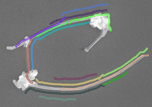
Figure 1: Example of the insufficient detection quality of CT-FIRE, when being applied to an image from the test data at hand. To reduce the number of false-positives, detections featuring a short fiber length were filtered with a threshold of $150\text{\,}\mathrm{p}\mathrm{x}$ (pixels). The remaining false-positive detections result from artifacts induced by the fast discrete CT used by CT-FIRE and could not be reduced any further through tuning of the associated parameters.

Due to these reasons, analyses of fiber length and width distributions still often have to be carried out manually. This practice is not only laborious, expensive and repetitive but also error-prone, due to the subjectivity and exhaustion of the operators [Allen.2003].

To solve these problems, we propose a new approach to fully automated imaging fiber analysis, with help of convolutional neural networks (CNNs). Recently, neural networks in general and CNNs in particular, have been applied successfully to particle measurement problems, such as the characterization of particle shapes and their size distribution [Frei.2020, Frei.2018, Heisel.2017, Heisel.2019, Wu.2020] as well as the classification of the chiral indices of CNTs [Forster.2020]. They are therefore promising candidates for the solution of the problem at hand. The main advantage of CNNs is that they require no user-tunable parameters, once they have been trained. Also, they are outstandingly robust to changes in imaging conditions. However, they require a set of already annotated samples for the training [Frei.2020].

Our previously presented, Mask R-CNN-based, particle analysis method [Frei.2020] works well for spherical instances, i.e. particles, even if they exhibit large amounts of occlusion and sintering. However, Mask R-CNN yields quite ragged instance masks, when being trained on and applied to fiber images (see Figure 2) and elongated objects in general [Looi.2019].

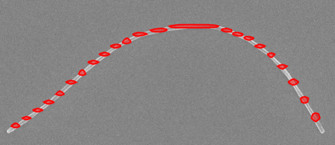
Figure 2: Example of the poor detection quality of Mask R-CNN, when being trained on and applied to fiber images from the test data at hand.

The Mask R-CNN architecture is region-based. Contrarily to spheres, fibers contribute only little information to the extracted region of interest (ROI) feature maps, due to their thinness and curvature and therefore small area relative to the area of their associated ROIs. Apparently, the extracted features do not suffice to reliably reconstruct the instance masks of the fibers directly.

However, we hypothesize that the features may be meaningful enough to extract keypoints, as well as widths and lengths of fibers. While the latter are often sought-after measurands themselves, their combination with the extracted keypoints also allows a more complete reconstruction of instance masks.

In this publication, we therefore propose, implement and validate an extension of the Mask R-CNN architecture, hereby named FibeR-CNN, to extract keypoints, widths and lengths of fibers from images, thereby improving automatic fiber shape analysis.

2 Training and Test Data

The fiber images used in this publication are courtesy of the Institute of Energy and Environmental Technology e.V. (IUTA) and were created using a JEOL JSM-7500F field emission scanning electron microscope (SEM). The pictured fibers are CNTs, deposited from the gas phase (see Figure 3).

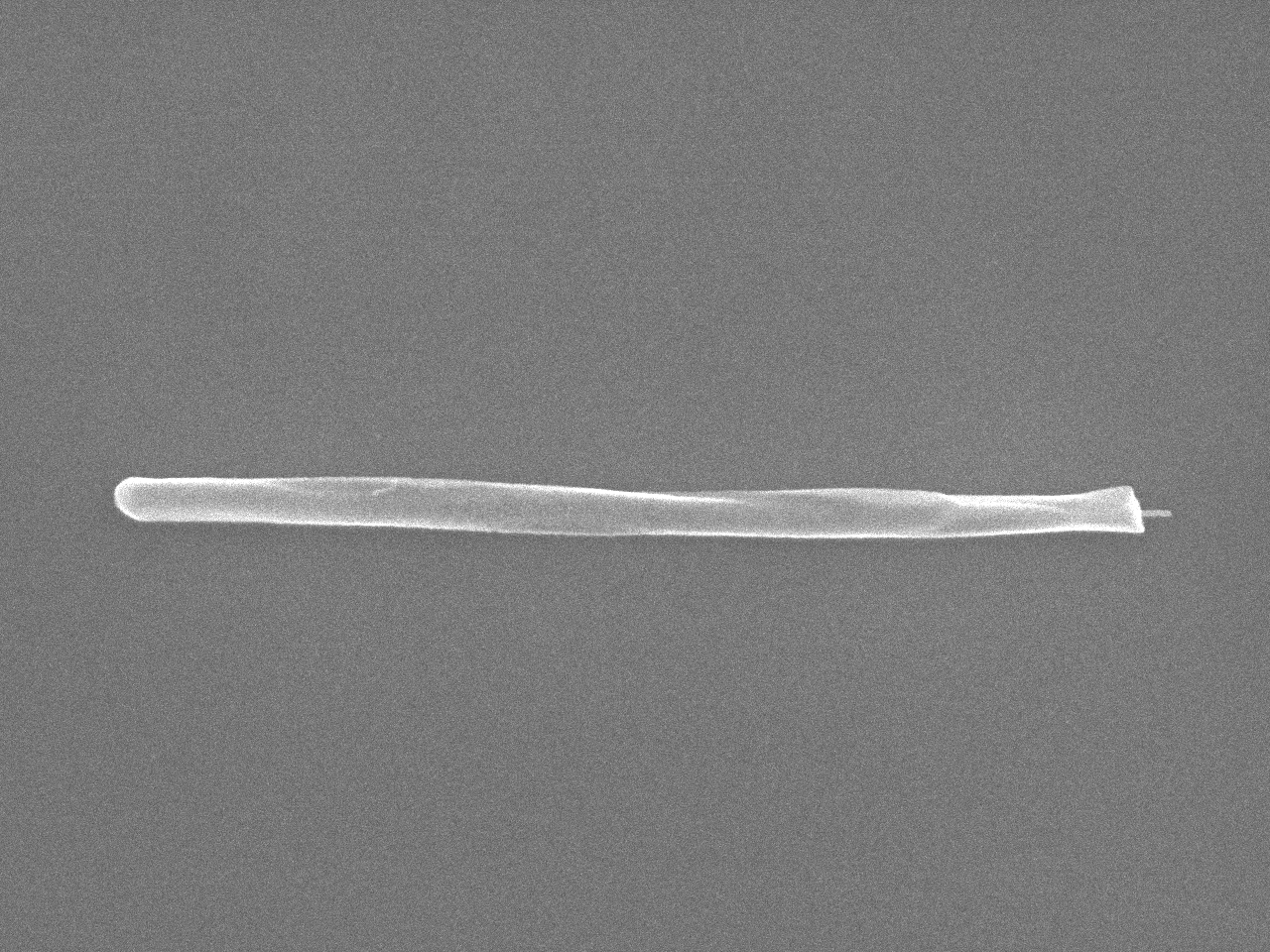
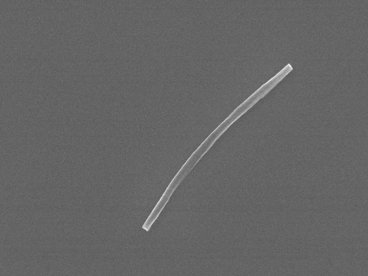
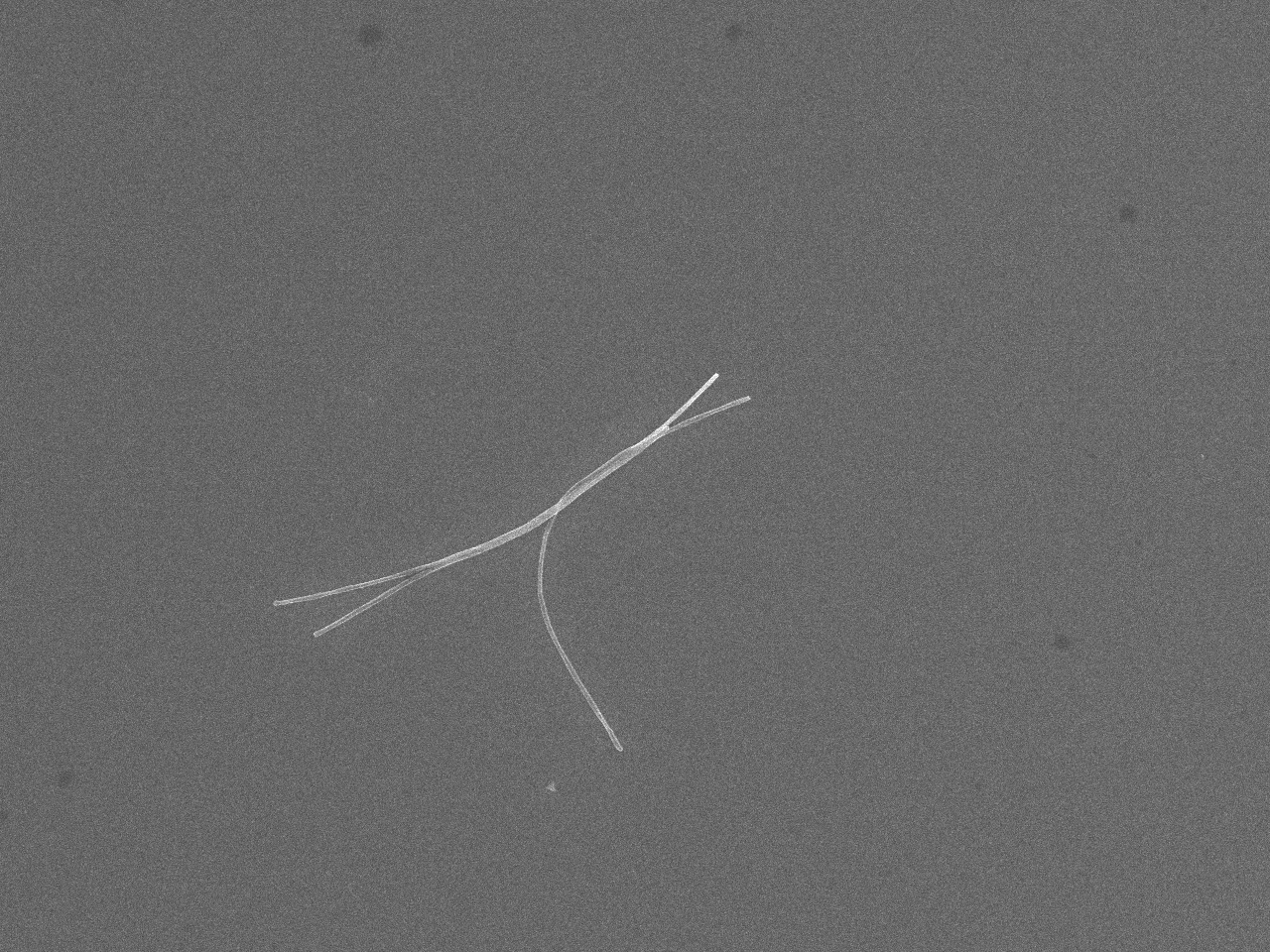
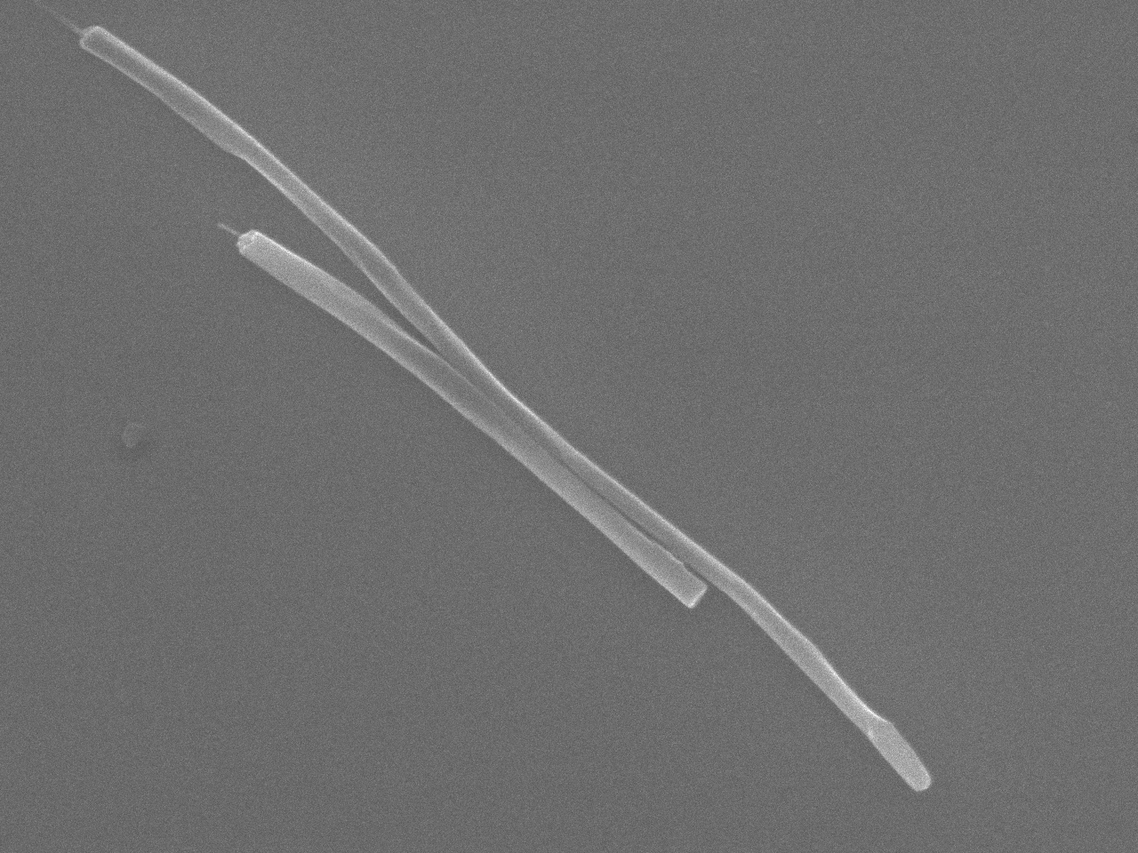
[-l|-c|-o]		[-l|-c|+o]
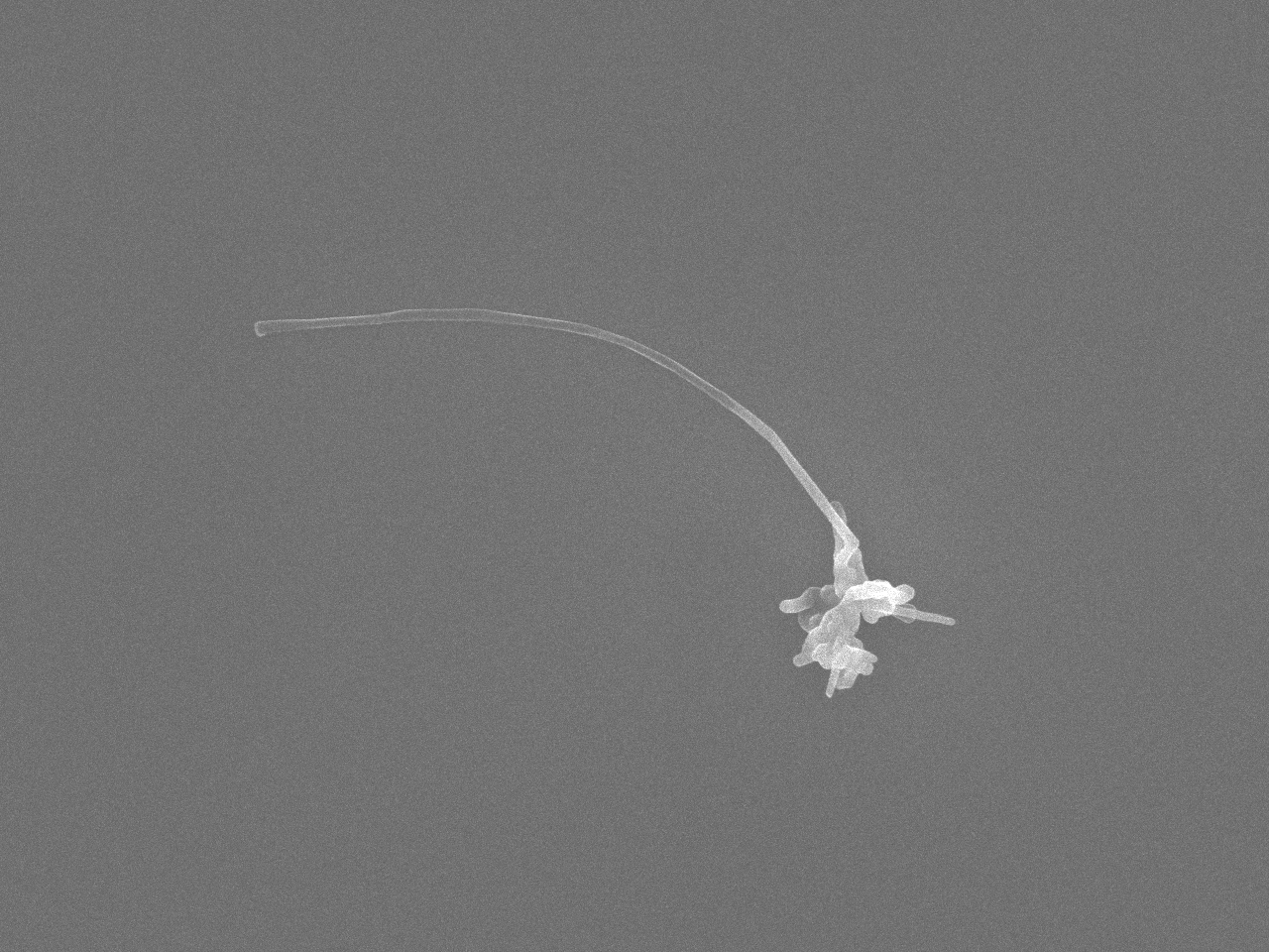
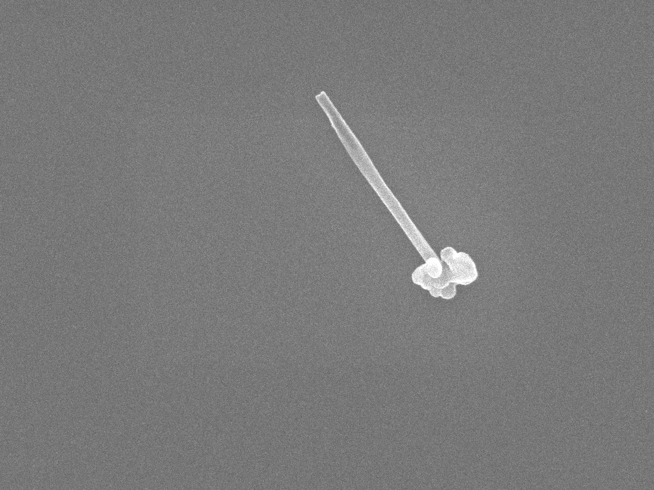
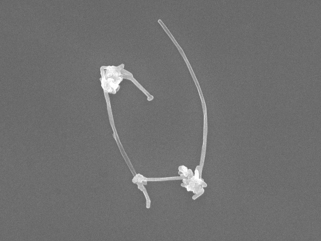
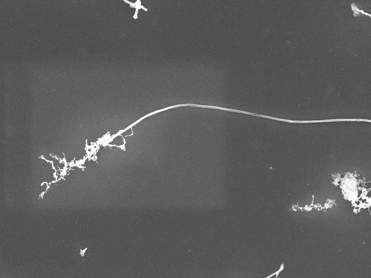
[-l|+c|-o]		[-l|+c|+o]
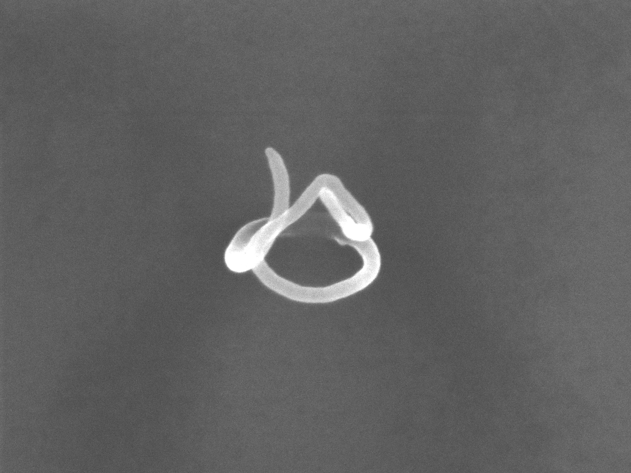
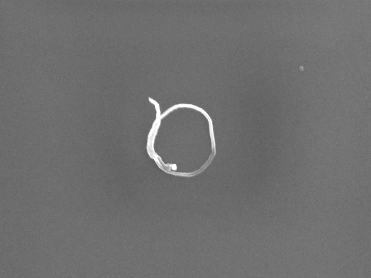
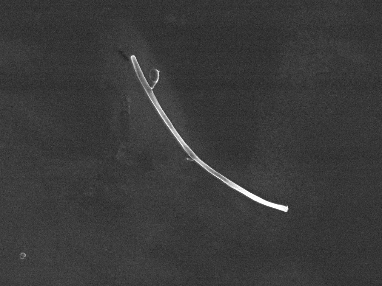
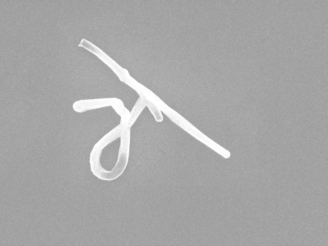
[+l|-c|-o]		[+l|-c|+o]
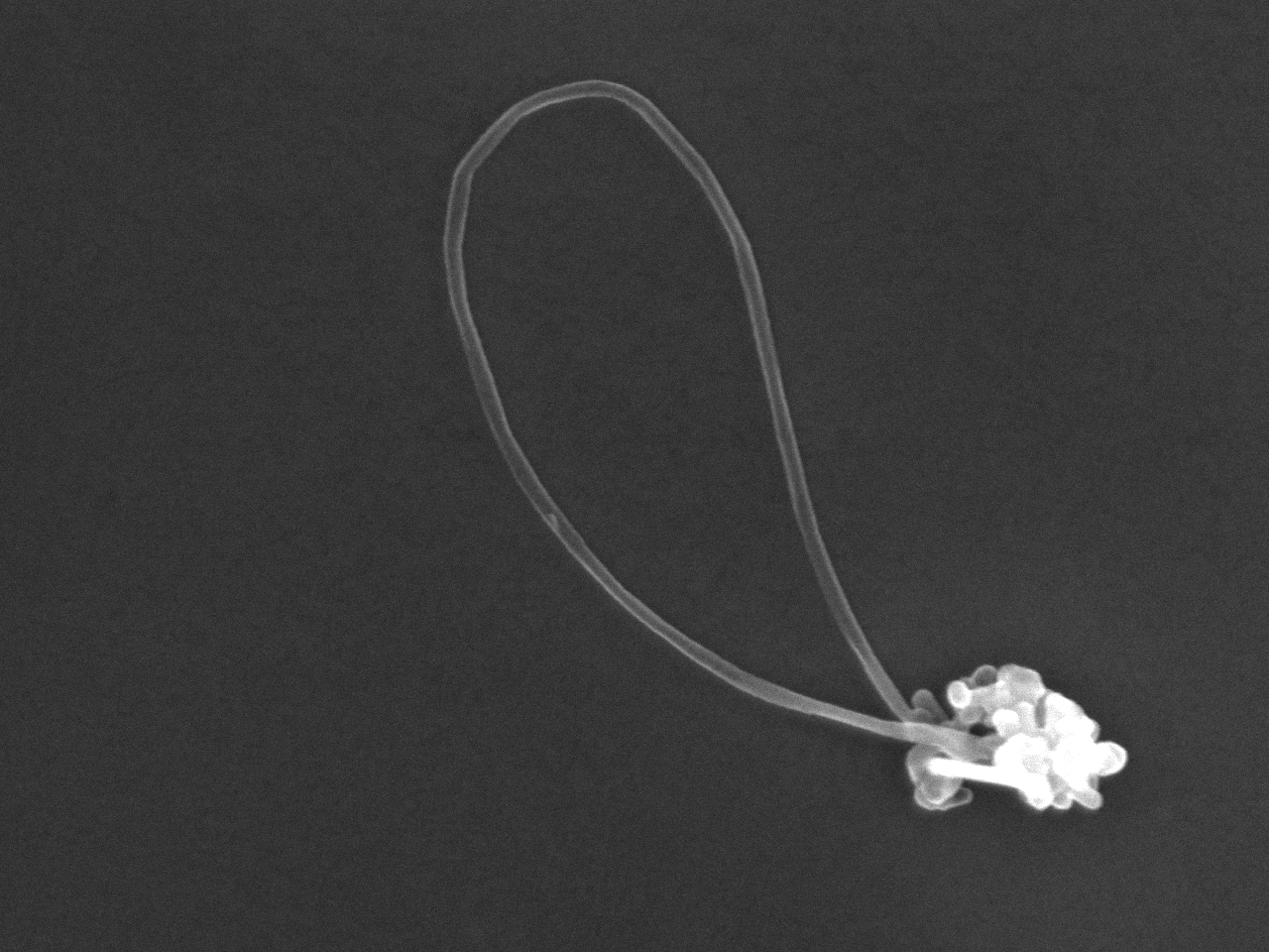
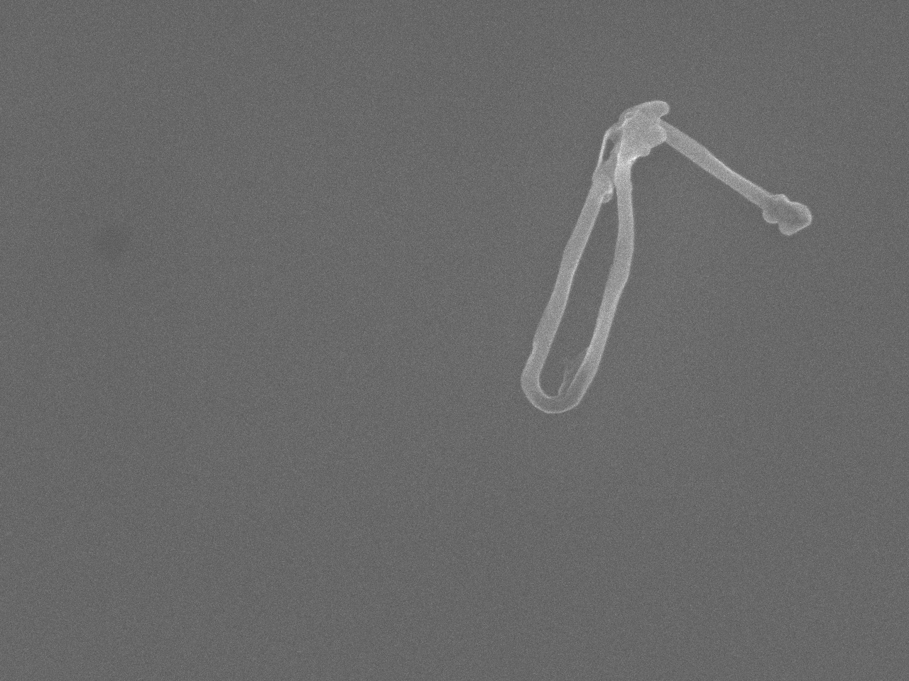
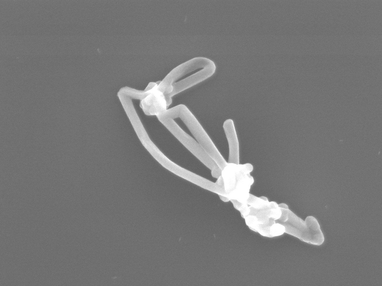
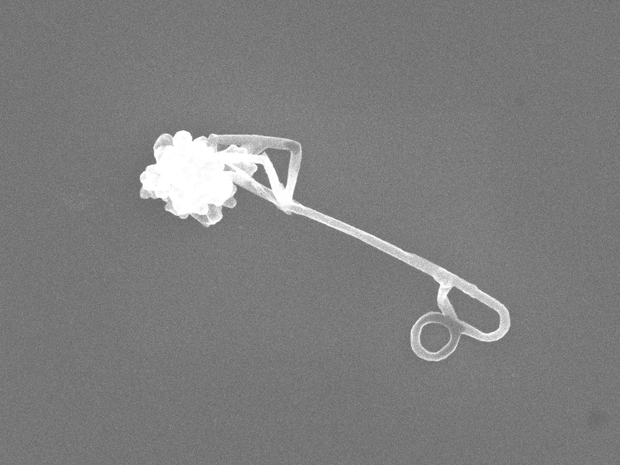
[+l|+c|-o]		[+l|+c|+o]
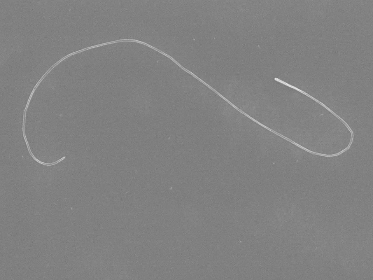
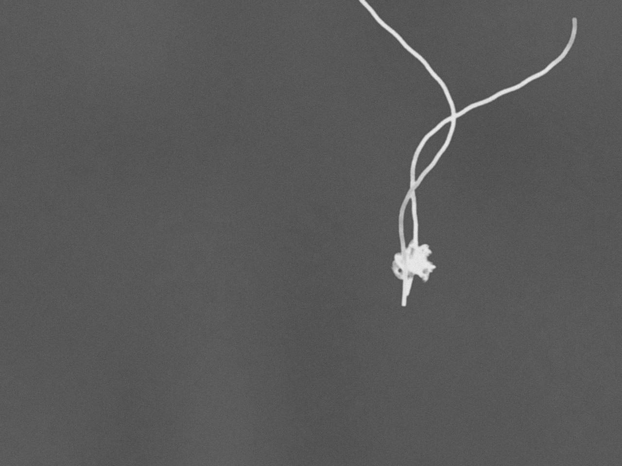
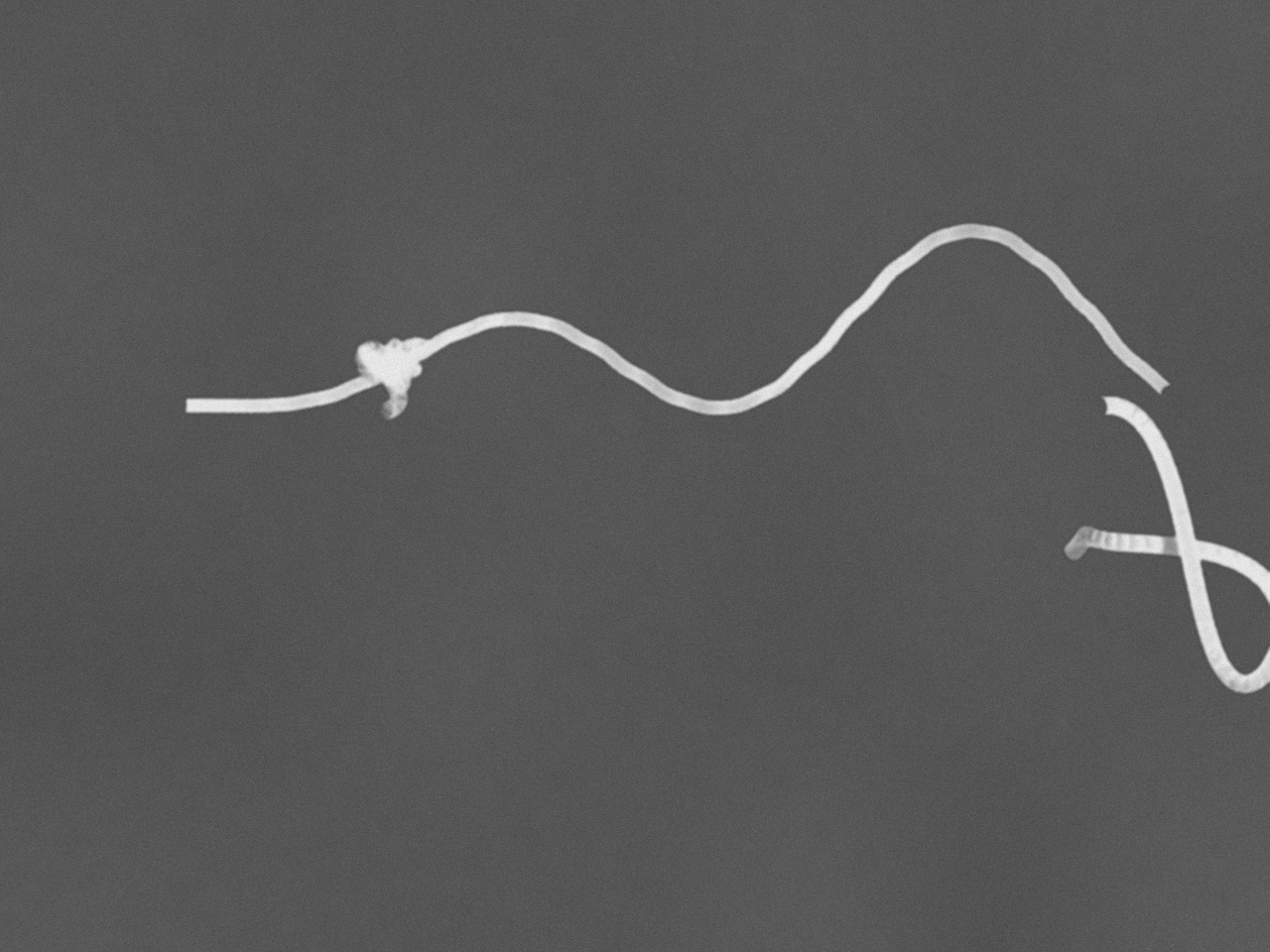
[-l|-c|-o]${}_{\text{auto.}}$		[?l|?c|?o]${}_{\text{synth.}}$

Figure 3: Example images of the utilized data sets (+/-/?: yes, no, random; l/c/o: loops, clutter, overlaps).

2.1 Ground Truth Generation

The ground truths, used to train and test the CNNs utilized within this publication, have three origins: manual annotation, semiautomatic annotation and image synthesis.

2.1.1 Manual Annotation

A total of $1075$ images, featuring $1935$ instances (i.e. fibers), were annotated manually, using an ad hocly implemented annotation tool. The manual annotation was done by selecting keypoints for each fiber that were interpolated using cubic splines and adjusting the fiber width until an optimal coverage was achieved (see Figure 4).

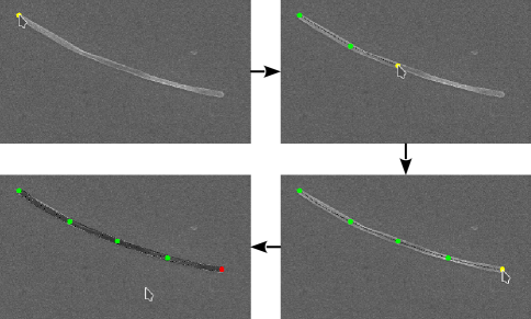
Figure 4: Illustration of the manual annotation process.

2.1.2 Semiautomatic Annotation

For basic fiber images, featuring neither clutter, loops nor overlaps (see Section 2.2), a semiautomatic annotation can be carried out to avoid the laborious task of manual annotation.

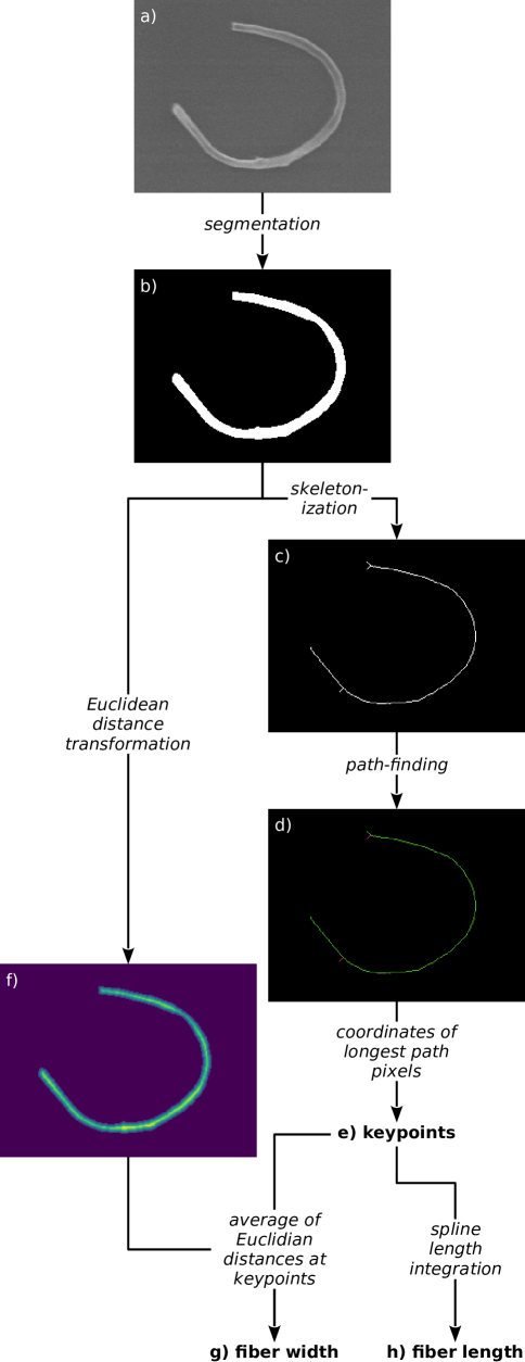
Figure 5: Illustration of the semiautomatic annotation process (see Section 2.1.2).

For the use case at hand, the semiautomatic annotation was implemented as follows (see also Figure 5):

1. The original image (see Figure 5a) is segmented using denoising and thresholding, yielding an instance mask (see Figure 5b).

2. The instance mask (see Figure 5b) is skeletonized (see Figure 5c).

3. To remove artifacts resulting from the skeletonization and to determine a correct order of keypoints, the longest connected path in the skeleton is identified via a path-finding method and all other pixels are discarded (see Figure 5d;   pixels: kept,   pixels: discarded).

4. The pixels of the longest connected path (see Figure 5d;    pixels) are converted into keypoint coordinates (see Figure 5e).

5. To determine the fiber width (see Figure 5g), an Euclidian distance map (see Figure 5f) of the instance mask (see Figure 5b) is calculated. Subsequently, the Euclidian distances of the previously determined keypoints (see Figure 5e) are looked up, their average is calculated and the resulting value is multiplied by a factor of $2$ to yield the fiber width.

6. The fiber length (see Figure 5h) is determined by integrating a cubic spline interpolation of the keypoints (see Figure 5e).

7. Finally, annotations with faulty keypoints or fiber widths are removed manually.

A total of $579$ images, featuring $583$ instances (i.e. fibers), were annotated semiautomatically.

2.1.3 Image Synthesis

Using our synthPIC toolbox, $500$ images, featuring 760 instances (i.e. fibers), were synthesized. The purpose of the synthetic images is to survey, whether they can be used to supplement or even replace real training data, thereby obliterating the need for a manual annotation.

2.2 Data Sets

So far, three data sets were distinguished: manually annotated, semiautomatically annotated and synthetic fiber images (see Section 2.1). However, the set of manually annotated images can be partitioned into subsets once again, based on the presence of potentially inhibiting factors for the automatic detection of fibers. A survey of the available images yielded three such factors:

• Loops: Self-overlapping fibers.

• Clutter: Agglomerates or aggregates of non-fiber particles which stick to fibers, e.g. nuclei that did not grow into long fibers.

• Overlaps: Multiple fibers which overlap each other. Fibers which are connected only by clutter are not considered overlapping.

The set of manually annotated images was therefore subdivided into eight subsets, representing all possible combinations of the three inhibiting factors (see Figures 3 and 1), to study their impact on the detection quality. Next, each real data set was partitioned once again, to yield training and test sets ($\lfloor$85\text{\,}\mathrm{\char 37\relax}$\rfloor/\lceil$15\text{\,}\mathrm{\char 37\relax}$\rceil$) for the proposed method (see Table 1, right side). Ultimately, due to the small number of images for data sets featuring loops, all loop data sets ([+l|...]; see Table 1, gray rows) were aggregated into a ninth data set ([+l|?c|?o]).

Table 1: Data set properties (+/-/?: yes, no, random; l/c/o: loops, clutter, overlaps). Gray rows represent data sets before aggregation.

					Number of Images			Number of Fibers
Loops	Clutter	Overlaps	Annotation	Identifier	Total	Training	Test	Total	Training	Test
no	no	no	manual	[-l|-c|-o]	$236$	$200$	$36$	$250$	$211$	$39$
no	no	yes	manual	[-l|-c|+o]	$107$	$90$	$17$	$227$	$192$	$35$
no	yes	no	manual	[-l|+c|-o]	$351$	$298$	$53$	$444$	$379$	$65$
no	yes	yes	manual	[-l|+c|+o]	$337$	$286$	$51$	$1014$	$855$	$159$
yes	random	random	manual	[+l|?c|?o]	$44$	$35$	$9$	$75$	$59$	$16$
yes	no	no	manual	[+l|-c|-o]	$22$	$18$	$4$	$23$	$19$	$4$
yes	no	yes	manual	[+l|-c|+o]	$2$	$1$	$1$	$5$	$3$	$2$
yes	yes	no	manual	[+l|+c|-o]	$11$	$9$	$2$	$13$	$11$	$2$
yes	yes	yes	manual	[+l|+c|+o]	$9$	$7$	$2$	$34$	$26$	$8$
no	no	no	semiautomatic	[-l|-c|-o]${}_{\text{auto.}}$	$579$	$492$	$87$	$583$	$496$	$87$
random	random	random	synthetic	[?l|?c|?o]${}_{\text{synth.}}$	$425$	$425$	–	$645$	$645$	–

3 Method

The focus of the proposed method lies on the modification of already existing R-CNN architectures (see Sections 3.1 and 3.2) and training schedules (see LABEL:sec:Method-Training), to meet the requirements of imaging fiber analysis. Furthermore, the proposed extensions require changes with respect to the preparation of the utilized input data (see Section 3.3) and allow for custom-designed error detection and correction strategies (see LABEL:sec:Method-ErrorDetectionAndCorrection).

3.1 Network Architecture

The FibeR-CNN architecture, presented within this publication, is an extension of the well-known Mask R-CNN architecture [He.2017] (see Figure 6;    box). It is therefore imperative to briefly elaborate upon the structure and general principles of Mask R-CNN. Subsequently, it will be expanded in two steps: Firstly, by adding a head for keypoint regression (see Figure 6;    box), thereby yielding the Keypoint R-CNN architecture [He.2017] and secondly, by adding two heads performing fiber width and length regressions, which ultimately yields the FibeR-CNN architecture (see Figure 6;    box).

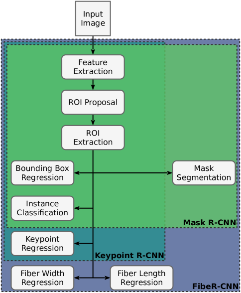
Figure 6: Architectures of Mask R-CNN, Keypoint R-CNN and FibeR-CNN.

As codebase for the implementation, the detectron2 framework [Wu.2019] was used, which features PyTorch [Paszke.2019] implementations of Mask R-CNN and Keypoint R-CNN.

3.1.1 Region-Based Convolutional Neural Networks

Modern R-CNNs consist of three conceptual stages (see Figure 7): feature extraction, ROI proposal/extraction and instance property prediction.

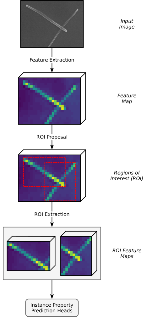
Figure 7: Illustration of the feature extraction as well as the ROI proposal and extraction, which are shared by most modern R-CNN architectures.

Feature Extraction

The input image is processed by a CNN, referred to as backbone, thereby extracting a map of prominent features over the entirety of the input image. Compared to the other architecture parts, the backbone is usually a much deeper network, i.e. it has more layers. Therefore, the majority of calculations takes place within the backbone. It is easily interchangeable to adjust the number of operations and thereby the network speed. In this publication, the convolutional blocks $25$ of the ResNet-50 network [He.2015] are used as backbone.

ROI Proposal and Extraction

ROIs encompassing instances are identified and extracted from the feature map. The ROIs are selected so that each ROI represents exactly one instance. Additionally, for each ROI an objectness score, which quantifies the likelihood of the ROI to encompass an object, is output. Subsequently, the set of instance feature maps is passed to each of the downstream heads, each of which predicts a desired instance property (e.g. class, bounding box, instance mask, keypoints, etc.).

Instance Property Prediction

R-CNNs can be distinguished based on the presence of characteristic instance property prediction heads (e.g. the mask segmentation or the keypoint regression head). However, most modern R-CNNs share at least two such heads: The bounding box regression head, which determines a refined bounding box for the instance in each ROI and the instance classification head, which determines the class of said instance. For the given application, the latter head is obsolete, because there is only a single class of instances. However, due to its negligible computational cost, it was not removed to facilitate future multi-class applications.

All instance property prediction heads operate on the same shared set of instance feature maps. Therefore, the computational cost of adding additional heads is small compared to the backbone’s computational cost. This is beneficial for the use-case at hand, since all extensions of Mask R-CNN within this publication come in the form of additional instance property prediction heads.

3.1.2 Mask R-CNN

The characteristic instance property prediction head of Mask R-CNN is the mask segmentation head (see Figure 6;    box), which computes a binary mask representing the instance pixels, i.e. it answers the question, which pixels of the input image belong to a certain instance and which pixels belong to the image background or another instance. Figure 8 illustrates the functionality of the mask segmentation: Initially, each ROI feature map, resulting from the ROI extraction, is resized using ROI align. Subsequently, a CNN upsamples the low-resolution, high-depth feature map to a high-resolution, low-depth binary mask.

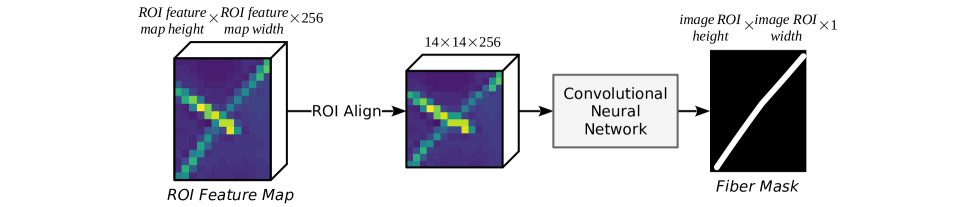
Figure 8: Illustration of the mask segmentation head.

3.1.3 Keypoint R-CNN

The Keypoint R-CNN architecture was proposed along with Mask R-CNN by He et al. [He.2017], with the task of human pose estimation in mind. Instead of a mask segmentation head, it features a keypoint regression head (see Figure 6;    box). The functionality of this head (see Figure 9) is closely related to that of the mask segmentation head (see Figure 8), with the key difference being that multiple (keypoint) masks per instance are predicted, instead of just a single mask. In each keypoint mask, there exists only a single true pixel, which represents the keypoint position.

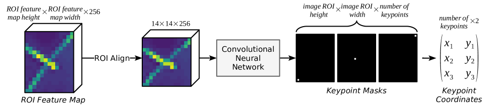
Figure 9: Illustration of the keypoint regression head (white pixels in keypoint masks are oversized).

In the original implementation, the keypoint regression head outputs the coordinates of $17$ keypoints, which is insufficient to describe the shapes of long and/or strongly curved fibers. Therefore, in the FibeR-CNN architecture, the keypoint regression head was altered to output 40 keypoint coordinates (see also Section 3.3.1), by increasing the respective dimension of its last layer.

3.1.4 FibeR-CNN

FibeR-CNN expands Mask R-CNN beyond Keypoint R-CNN by adding two additional instance property prediction heads (see Figure 6;    box): the fiber width and length regression heads.

The architectures of these heads were inspired by the bounding box regression head of Mask R-CNN [He.2017], i.e. they are implemented as fully connected neural networks, which each consist of three rectified linear unit (ReLU) layers (see Figure 10). As inputs for the fully connected neural networks, resized and flattened versions of the input ROI feature maps are used. In contrast to the mask and keypoint prediction heads, the fiber width and length regression heads – just like the bounding box regression head – operate on lower-resolution versions of the utilized ROI feature maps, to reduce the size and complexity of the utilized fully connected neural network. During the flattening, each multidimensional ROI feature map is transformed into a vector by concatenating all of its elements. Subsequently, each element is being fed to a corresponding input neuron of the downstream fully connected neural network, which, as a whole, predicts the fiber width or length, respectively.

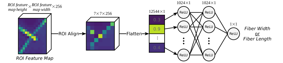
Figure 10: Architecture of the fiber width and fiber length regression head, respectively.

Due to the fact that the fiber width, as well as the fiber length regression head both only output a single quantity, each of them only features a single output neuron. While the prediction of a single length per fiber is intuitive, the prediction of just a single width per fiber is arbitrary and tailored to the utilized data, which features only fibers with various, yet constant widths. However, for fibers with inconstant widths, the architecture could easily be expanded, by adding more output neurons to the fiber width regression branch, to predict an individual width at every keypoint.

At first glance, the mask segmentation head inherited from the Mask R-CNN architecture and the fiber length head may seem obsolete. After all, a fiber mask can also be attained by performing a cubic spline interpolation of the detected fiber keypoints and drawing this spline with lines having the predicted fiber width. Similarly, the fiber length can be determined by performing an integration of the cubic spline approximation. However, actually, these redundancies are indeed useful, because they enable the application of error detection and correction strategies (see LABEL:sec:Method-ErrorDetectionAndCorrection), to improve the detection accuracy.

3.2 Loss Function

The loss function – sometimes also referred to as cost function – is an essential element of many optimization problems, such as the training of neural networks. It is a means to quantify the quality of a model, based on the deviation of its predictions from the ground truth, i.e. the desired target outputs. The higher the deviation, the higher the loss. Therefore, the goal of the training is to minimize this loss.

FibeR-CNN uses a multi-task loss $\mathcal{L}$, which is equal to the sum of the individual prediction head losses:

$$\lx@glossaries@gls@link{symbolslist}{symb:loss}{\leavevmode\mathcal{L}}=\lx@glossaries@gls@link{symbolslist}{symb:lossClass}{\leavevmode\mathcal{L}_{\text{cls}}}+\lx@glossaries@gls@link{symbolslist}{symb:lossBox}{\leavevmode\mathcal{L}_{\text{box}}}+\lx@glossaries@gls@link{symbolslist}{symb:lossMask}{\leavevmode\mathcal{L}_{\text{mask}}}+\lx@glossaries@gls@link{symbolslist}{symb:lossKeypoint}{\leavevmode\mathcal{L}_{\text{kp}}}+\lx@glossaries@gls@link{symbolslist}{symb:lossWidth}{\leavevmode\mathcal{L}_{\text{fw}}}+\lx@glossaries@gls@link{symbolslist}{symb:lossLength}{\leavevmode\mathcal{L}_{\text{fl}}}$$ (1)

$\mathcal{L}_{\text{cls}}$ and $\mathcal{L}_{\text{box}}$ are the instance classification and bounding box regression head losses [Girshick.2015], whereas $\mathcal{L}_{\text{mask}}$ and $\mathcal{L}_{\text{kp}}$ are the mask segmentation and keypoint regression head losses [He.2017].

The fiber width and length prediction head losses $\mathcal{L}_{\text{fw}}$ and $\mathcal{L}_{\text{fl}}$ are both based on the mean squared error (MSE):

$$\lx@glossaries@gls@link{symbolslist}{symb:lossWidth}{\leavevmode\mathcal{L}_{\text{fw}}}(\lx@glossaries@gls@link{symbolslist}{symb:prediction}{\leavevmode y},\lx@glossaries@gls@link{symbolslist}{symb:target}{\leavevmode t})=\lx@glossaries@gls@link{symbolslist}{symb:lossWeightWidth}{\leavevmode w_{\text{fw}}}\cdot\lx@glossaries@gls@link{symbolslist}{symb:meanSquaredError}{\leavevmode\text{MSE}}(\lx@glossaries@gls@link{symbolslist}{symb:prediction}{\leavevmode y},\lx@glossaries@gls@link{symbolslist}{symb:target}{\leavevmode t})$$ (2)

$$\lx@glossaries@gls@link{symbolslist}{symb:lossLength}{\leavevmode\mathcal{L}_{\text{fl}}}(\lx@glossaries@gls@link{symbolslist}{symb:prediction}{\leavevmode y},\lx@glossaries@gls@link{symbolslist}{symb:target}{\leavevmode t})=\lx@glossaries@gls@link{symbolslist}{symb:lossWeightLength}{\leavevmode w_{\text{fl}}}\cdot\lx@glossaries@gls@link{symbolslist}{symb:meanSquaredError}{\leavevmode\text{MSE}}(\lx@glossaries@gls@link{symbolslist}{symb:prediction}{\leavevmode y},\lx@glossaries@gls@link{symbolslist}{symb:target}{\leavevmode t})$$ (3)

where

$$\lx@glossaries@gls@link{symbolslist}{symb:meanSquaredError}{\leavevmode\text{MSE}}(\lx@glossaries@gls@link{symbolslist}{symb:prediction}{\leavevmode y},\lx@glossaries@gls@link{symbolslist}{symb:target}{\leavevmode t})=\frac{1}{\lx@glossaries@gls@link{symbolslist}{symb:numberOfDates}{\leavevmode n}}\sum_{\lx@glossaries@gls@link{symbolslist}{symb:index}{\leavevmode i}=1}^{\lx@glossaries@gls@link{symbolslist}{symb:numberOfDates}{\leavevmode n}}(\lx@glossaries@gls@link{symbolslist}{symb:prediction}{\leavevmode y}_{\lx@glossaries@gls@link{symbolslist}{symb:index}{\leavevmode i}}-\lx@glossaries@gls@link{symbolslist}{symb:target}{\leavevmode t}_{\lx@glossaries@gls@link{symbolslist}{symb:index}{\leavevmode i}})^{2}$$ (4)

is the mean squared error, $y$ and $t$ are the prediction and target vectors of the respective heads, $i$ is the index of each instance and $n$ is the number of dates, i.e. instances.

The main difference of the losses are their weights $\lx@glossaries@gls@link{symbolslist}{symb:lossWeightWidth}{\leavevmode w_{\text{fw}}}=${10}^{-3}$$ and $\lx@glossaries@gls@link{symbolslist}{symb:lossWeightLength}{\leavevmode w_{\text{fl}}}=${10}^{-6}$$, which where chosen so that $\mathcal{L}$ is not dominated by the fiber width and length regression heads. In practice, the weights wfw and wfl were adjusted, so that all prediction head losses have a similar magnitude at the beginning of the training:

$$\lx@glossaries@gls@link{symbolslist}{symb:lossClass}{\leavevmode\mathcal{L}_{\text{cls}}}\sim\lx@glossaries@gls@link{symbolslist}{symb:lossBox}{\leavevmode\mathcal{L}_{\text{box}}}\sim\lx@glossaries@gls@link{symbolslist}{symb:lossMask}{\leavevmode\mathcal{L}_{\text{mask}}}\sim\lx@glossaries@gls@link{symbolslist}{symb:lossKeypoint}{\leavevmode\mathcal{L}_{\text{kp}}}\sim\lx@glossaries@gls@link{symbolslist}{symb:lossWidth}{\leavevmode\mathcal{L}_{\text{fw}}}\sim\lx@glossaries@gls@link{symbolslist}{symb:lossLength}{\leavevmode\mathcal{L}_{\text{fl}}}$$ (5)

Otherwise, the neural network would focus primarily on the improvement of the fiber width and length prediction heads heads and neglect the other heads during the training. This could for instance result in a network which can very reliably predict fiber widths and lengths, but not bounding boxes or keypoints.

3.3 Data Transformations

To homogenize or augment the input and ground truth data of CNNs, it is often useful or even mandatory to apply transformations to it.

3.3.1 Number of Keypoints

As mentioned in Section 3.1.3, the number of keypoints per instance, predicted by the keypoint regression head of FibeR-CNN, had to be adjusted, to yield a high enough resolution of keypoints, to describe the shape of long and/or strongly curved fibers. Also, the calculation of the keypoint regression head loss requires a consistent number of keypoints in the ground truths.

While a higher number of keypoints yields a better resolution, as with all statistical models, it is undesirable to introduce more degrees of freedom (i.e. keypoints) than necessary. Therefore, approximations of the ground truth, using varying numbers of keypoints were tested and the resulting approximation qualities were assessed using the Bayesian information criterion (BIC) .

According to Yaffee and McGee [Yaffee.2000], the BIC (omitting the Bessel’s correction [Radziwill.2017]) is defined as:

$$\text{<span title="" class="ltx\_glossaryref">BIC</span>}(\text{<span title="" class="ltx\_glossaryref ltx\_font\_italic">y</span>},\text{<span title="" class="ltx\_glossaryref ltx\_font\_italic">t</span>})=\text{<span title="" class="ltx\_glossaryref ltx\_font\_italic">n</span>}\cdot \ln (\frac{1}{\text{<span title="" class="ltx\_glossaryref ltx\_font\_italic">n</span>}}\cdot \text{<span title="" class="ltx\_glossaryref">SSR</span>}(\text{<span title="" class="ltx\_glossaryref ltx\_font\_italic">y</span>},\text{<span title="" class="ltx\_glossaryref"><span class="ltx\_text ltx\_glossary\_name"><xmath xmlns="http://dlmf.nist.gov/LaTeXML" id="S3.E6.m1.1.18d" xref="S3.E6.m1.1.18f.cmml"><xmtok role="UNKNOWN" font="italic" id="S3.E6.m1.1.18e" xref="S3.E6.m1.1.18f.cmml">t</xmtok></xmath></span></span>}$$ (6)