Cracking the Black Box: Distilling Deep Sports Analytics

Abstract.

This paper addresses the trade-off between Accuracy and Transparency for deep learning applied to sports analytics. Neural nets achieve great predictive accuracy through deep learning, and are popular in sports analytics (Fernández et al., 2019; Liu and Schulte, 2018; Burke, 2019; Wang et al., 2018). But it is hard to interpret a neural net model and harder still to extract actionable insights from the knowledge implicit in it. Therefore, we built a simple and transparent model that mimics the output of the original deep learning model and represents the learned knowledge in an explicit interpretable way. Our mimic model is a linear model tree, which combines a collection of linear models with a regression-tree structure. The tree version of a neural network achieves high fidelity, explains itself, and produces insights for expert stakeholders such as athletes and coaches. We propose and compare several scalable model tree learning heuristics to address the computational challenge from datasets with millions of data points.

1. Introduction

Both neural networks and tree-based method are widely used in machine learning and sports analytics (Liu and Schulte, 2018; Fernández et al., 2019; Burke, 2019; Wang et al., 2018) to obtain actionable information. They can provide predictions for not just hypothetical situations but counterfactual ones as well. If one is using either method to estimate the chance of a shot in ice hockey or soccer resulting in a goal, and that method uses variables like “distance to the net”, “number of players between the shooter than the net”, and “type of shot”, then one can use the model to ask questions like “what happens if the shooter performs a chip shot instead of a standard shot?” or “how much greater is the success chance if I cut the distance to the net by half?”. There are two operative differences in these predictions between trees and neural networks, predictive accuracy and transparency.

Without introducing a great deal of complexity, trees are weak classifiers and regressors; they leave a lot of variance unexplained or cases mis-classified. When there is enough complexity for a tree to make good regressions or classifications, the resultant tree over overfits the data it was trained on. Furthermore, trees can be sensitive to small changes in the training data. This instability is serious enough that trees are rarely taken alone and instead are used in random forests (Ho, 1995), which are ensembles of trees in which each tree is trained on a subset of the variables and observations available. By comparison, neural networks are strong predictors. They typically produce predictive values that are much closer to reality, even on new, similar, observations that weren’t part of the training data. Neural networks are much better than trees in terms of output quality.

Transparency is the other major difference: to apply predictions to a tree, simply start at the top of the tree and apply the decision rules until a leaf is reached. It is clear why a particular prediction was made, and what variables contributed to that prediction. Counterfactual predictions can be applied in the same way. Therefore, a tree model is transparent. By contrast, neural networks are black boxes: there is no clear path between any one variable and its effect on predictions. After a couple of intermediate layers of neurons, every input variable can have a non-trivial and non-obvious effect on the output. To explore counter-factual possibilities, it is necessary to run a set of variable values through the entire neural network, rather than examine any small piece. Neural networks are opaque.

This tradeoff between accuracy and transparency poses a major problem in sports analytics. We are often confronted with a great deal of variables and observations from which we need to make high quality predictions, and yet we need to make these predictions in such a way that it is clear which variables need to be manipulated in order to increase a team or single athlete’s success.

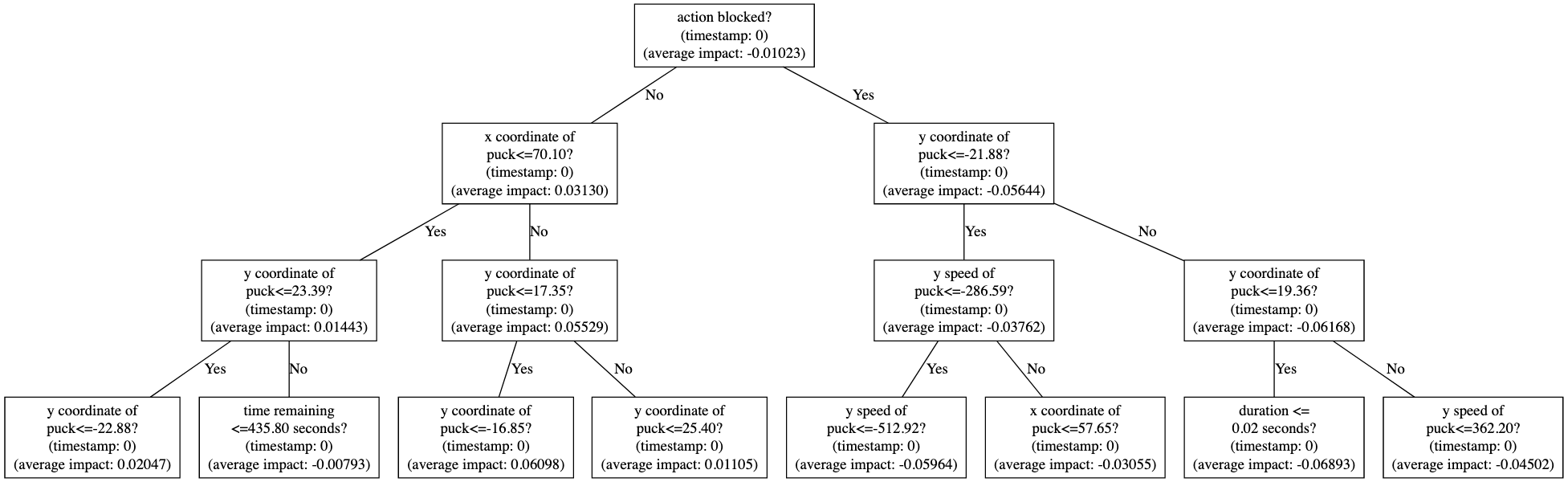
Figure 1. Model Tree Example With 4 Layers for Impact of Shots in Ice Hockey

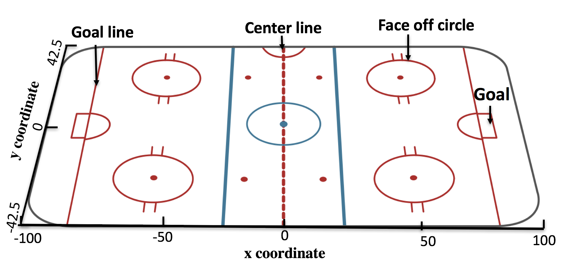
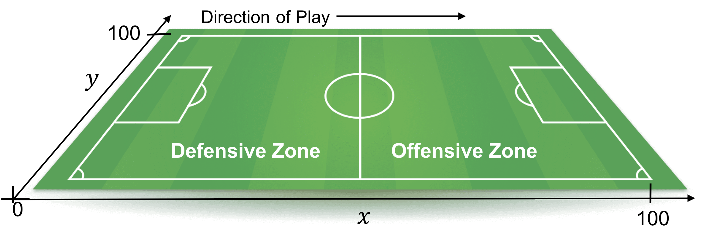
Figure 2. Ice Hockey Rink and Soccer Field With Coordinates

Mimic Learning is an approach that aims to get the best of both worlds: transparency without sacrificing an acceptable degree of accuracy. The basic idea is to learn an accurate black-box model, like a deep reinforcement learning (DRL) model with neural net, then train a transparent white-box model, like a regression tree, to mimic the black-box model, thereby inheriting much of the predictive accuracy. Mimic learning with tree models can be seen as knowledge extraction from a trained neural net: The tree thresholds on predictive features represent critical values for predicting response variable. It is easy to compute a feature importance metric from the tree. This informs the user which features are most influential for the neural network predictions. Finally, a mimic tree extracts rules as if-then combinations of game state features provide information about how the important features interact with each other to influence sports outcomes.

To demonstrate our work, one set of mimic trees is trained to predict this action-value for passes and shots in ice hockey and soccer. Our evaluation shows that our algorithms are computationally feasible (returning an answer in less than a day even on very large datasets) with great fidelity. Although we conduct experiments in sports, mimic learning with model trees is a general technique and can be applied to other domains. We also build mimic trees to predict the impact of these actions, which measures how much an action changes a team’s expected success.

Contributions: While mimic learning has been explored in machine learning (Ba and Caruana, 2014; Che et al., 2016; Dancey et al., 2007), to our knowledge it is new to sports analytics. Dense sports datasets can easily contain millions of data points. For example, our study uses a hockey dataset and a soccer dataset with more than seven million data points. As mentioned in section 6, standard tree learning packages fail to process such large datasets. To address this severe computational challenge, we develop scalable model tree learning methods. The key is fast heuristic methods for finding promising thresholds for continuous predictor features (or co-variates). We also introduce a new data augmentation technique appropriate for counterfactual strategic settings.

2. Previous Work

Previous works on mimic learning have demonstrated that it is possible to learn a simple model, such as a shallow neural network (Ba and Caruana, 2014) or a tree-based model (Dancey et al., 2007), from an opaque complex model, such as a deep neural network, and maintain a similar predictive accuracy as the complex model. It has been shown that by doing so the prediction accuracy of the simple model outperforms the same simple model trained directly on the training set (Ba and Caruana, 2014). Our work introduces three novel ideas that are important for action-value functions. (1) Whereas previous work uses simple regression trees for mimicking neural networks with continuous outputs, we use a linear model tree. Our experiments show that the additional expressive power of model trees compared to regression trees is essential for complex functions like expected success values in team sports. This agrees with the very recent work by (Liu and Schulte, 2018), who found that model trees are key for representing value functions in general reinforcement learning problems. (2) We investigate several fast heuristic methods for building model trees. These heuristics are crucial for both computational feasibility and fidelity. (3) We introduce action replacement, a new data augmentation technique for sports data.

We apply mimic learning to construct interpretable models for action-value and impact functions. An action-value function, which is also called a Q-function, $Q(S_{t},A_{t})$ estimates the expected future success of a team given the current match state $S_{t}$ and the current action $A_{t}$. For example, in the hockey model of (Schulte et al., 2017), $Q(S_{t},A_{t})$ represents the conditional probability of a given team scoring the next goal given the event history (the state $S_{t}$) and the current action $A_{t}$. Other examples of action-value functions in sports analytics include expected points value (EPV) for basketball (Cervone et al., 2014), expected possession value in soccer (Fernández et al., 2019), and expected points in NFL football (Yurko et al., 2019). These studies have shown that action-values are a powerful way of valuing decisions and ranking players. However, the action-value function is not easy to interpret for sports stakeholders as it involves an expectation over future match trajectories. When the action-value function is estimated using neural nets, it is opaque to the user how it is computed (Fernández et al., 2019; Liu and Schulte, 2018). The combination of intransparency with usefulness makes the action-value function a suitable challenge for evaluating our mimic learning framework.

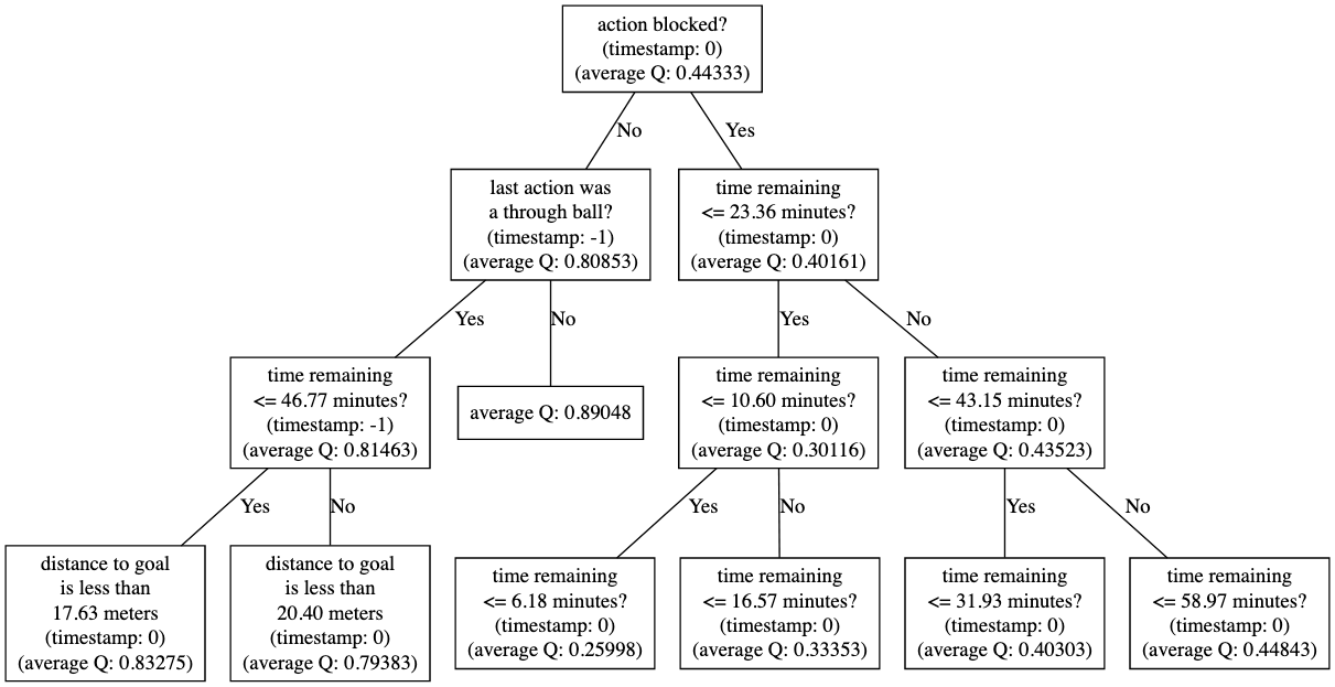
Figure 3. Model Tree Example With 4 Layers for Action-Value of Shots in Soccer

Mimic learning translates a black-box model into a white-box model. An alternative approach is to analyze the neural net directly as a black box (Guidotti et al., 2019). A representative example of a black-box approach is Dalex (Biecek, 2018). Dalex utilizes different types of plots to visualize the behavior of a black-box model. For example, it performs residual diagnostics to analyze a regression model by drawing a plot that contains both the predictions of the model and their actual labels. Then, it is clear to spot the places where the model makes mistakes. Partial dependence plots show how the dependent variable changes if we change only one independent variable at a time. Also, Dalex and other explanation methods have been developed so far only for supervised regression and classification models (Biecek, 2018), not reinforcement learning.

We believe that converting a black-box model to a white-box model tree has two key advantages for sports analytics. (1) The model tree provides a comprehensive analysis of relevant interactions among domain variables. Interactions are represented in an intuitive visual tree format, so that even complex combinations of features remain comprehensible. (2) The mimic model can guide the user towards especially interesting and useful phenomena gleaned from the data. We illustrate this technique of “mining the model” in our examples below.

Figure 4. Model Tree Learned From a Biased DRL Model for Ice Hockey

3. Dataset and Neural Network Architecture

3.1. Input Features

The data we used to conduct these experiments are collected by Sportlogiq. The data provides information about ice hockey game matches in the 2018-2019 NHL season and soccer game matches in the 2017-2018 season covering 10 leagues. Each data point represents a discrete event in a game, which combines information about the current situation and an action performed by a player on a team. Table 2 lists all the input variables for ice hockey and soccer, and Figure 2 provides the visual demonstration of how coordinate systems are defined. In ice hockey, the x and y coordinates of puck are measured in feet from center ice, where -100 and 100 in the x-coordinate represent the planes at the backboards behind each net respectively, and -42.5 and 42.5 represent the planes at the boards at the sides with the players’ benches and penalty boxes respectively. The x coordinates on the defensive zone of a team are negative and that on the offensive zone are positive. In soccer, field length and width are evenly divided into 100 units, where coordinates (50, 50) represents the center spot of the field, (0, 50) and (100,50) represent the nets on the defensive zone and the offensive zone, respectively. In both ice hockey and soccer, the angle between the puck/ball and the goal is measured in radians clockwise from directly in front, such that $+\pi$, $-\pi$, $+\pi/2$, $-\pi/2$, are directly to the front, back, right and left of the net, respectively. The data also contain variables that specify actions and are normalized before being used for training.

Table 1. Fidelity to Deep Model: RMSE on Test Set

	Ice Hockey				Soccer
	Shots		Passes		Shots		Passes
Split methods	action-values	impacts	action-values	impacts	action-values	impacts	action-values	impacts
Gaussian Mixture	0.05483	0.01990	0.04276	0.00687	0.00698	0.01312	0.01000	0.00577
Iterative Segmented Regression	0.01441	0.01999	0.00964	0.00691	0.00508	0.01275	0.00997	0.00575
Sorting + Variance Reduction	0.01219	0.01627	0.01012	0.00686	0.00646	0.01235	0.01092	0.00603
Sorting + T-test	0.05709	0.02487	0.06695	0.00935	0.01223	0.01377	0.01796	0.00597
Null Model	0.13924	0.05688	0.10808	0.01756	0.13648	0.11890	0.06151	0.00961

3.2. Target variable: Action Values and Impact Values

To generate “soft” labels for the mimic model, the neural net model outputs three action-values for each state and action pair $(S_{t},A_{t})$. The first action-value represents the probability of the home team having the next goal, the second action-value represents the probability of the away team having the next goal, and the third action-value represents the probability that the game ends before either team scores again.

Another important quantity is action impact (Liu and Schulte, 2018). Impact is defined as the difference between the action-value of a team given the current state-action pair and the action-value of the team given the previous state-action pair

$$Impact(S_{t},A_{t})=Q(S_{t},A_{t})-Q(S_{t-1},A_{t-1}).$$

Impact represents the amount that an action performed by a player changes the probability of a given team scoring the next goal given the previous state. It is a useful refinement of action-values for measuring the importance of a specific action, by controlling for the general scoring chances of a team, which may not be under the control of the acting player. For example, in an empty net situation, the team driving towards the empty net has a high chance of scoring, which translates into a high action-value. But a player scoring on an empty net should not be given higher credit than for other goals. Therefore the previous works cited use the impact concept or a version of it to value actions and players, often called $<$metric$>$-added, e.g. EPV-added (Cervone et al., 2014; Schulte et al., 2017; Yurko et al., 2019). In our evaluation, we carry out mimic learning for both the action-value and impact target variables.

3.3. Deep Reinforcement Learning Model

Refer to (Liu and Schulte, 2018), the neural network architecture we use to construct the DRL model consists of five layers: an input layer, an LSTM hidden layer, two fully connected hidden layers and an output layer. Each hidden layer has 1000 ReLU neurons. Each game match is divided into episodes, such that each episode starts with either the beginning of a period or immediately after a team scoring a goal, and ends with either the end of a period or immediately when a team scoring a goal. We apply SARSA (Rummery and Niranjan, 1994), an on-policy temporal difference learning method ($\lambda=1$), to the episodic dataset to estimate a Q-function. The parameters of the DRL model are optimized using minibatch gradient descent via Backpropagation Through Time with a fixed window-size of 10. The loss and update functions can be formulated as

$$\mathcal{L}_{t}(\theta_{t})=\mathbb{E}[(R_{t}+\hat{Q}(S_{t+1},A_{t+1};\theta_{t})-\hat{Q}(S_{t},A_{t};\theta_{t}))^{2}]$$

$$\theta_{t+1}=\theta_{t}-\alpha\cdot\nabla_{\theta}\mathcal{L}_{t}(\theta_{t})$$

where $R_{t}$ is the reward at time step $t$, $\theta_{t}$ are parameter values at time step $t$, and $\alpha$ is the learning rate.

3.4. Linear Model Tree Examples

Figure 1 shows the first 4 layers of a shot impact model tree for ice hockey. To be consistent with the DRL model, the tree is also learned with a 10-step window of events preceding the current action, so predictor variables are shown with timestamps, where 0 indicates that the variable belongs to the same time $t$ as the current action $A_{t}$. As observations from the same time as the action are the most relevant to predicting its impact, the top layers of the tree split only on features with timestamp 0. The tree can be read in a top-down manner. The root node shows the first split condition and the average of the impact values in the training set. For each split, if the split condition is true, we follow the left edge to the next node; otherwise, we follow the right edge instead. For example, if the shot is blocked, then the tree checks the y-coordinate. If the shot occurred from more than 21.88 y-feet away, it checks the y-speed. Similarly, Figure 3 shows the top 4 layers of a shot action-value (Q-value) model tree for soccer. The soccer tree also first splits on whether the shot is blocked or not. If the shot is blocked, then the tree checks if the last action before the shot was a through ball. For every child node, there is a new set of records assigned to the child node, and accordingly, a new average on every child node. When a leaf node is reached, a linear model is used to predict a target value.

$$\hat{y}=(\sum_{i}w_{i}\cdot x_{i})+b$$

We can think of the conjunction of conditions along a branch as defining a discrete subset of the continuous input space (Uther and Veloso, 1998).

4. Model Tree Learning Outline

In this section we outline our mimic learning method, emphasizing the novel contributions that support tree learning for sports analytics. We first describe our data augmentation, then the novel aspects of our method and how it supports learning interpretable trees. We provide our code available on-line .

4.1. Data Augmentation

An important strength of mimic learning is the ability to generate “soft” labels for unobserved data points (sometimes called oracle coaching (Johansson et al., 2014)) from the black-box model. This can be seen as a form of data augmentation. It is well-known that neural networks can be viewed as interpolating output labels (Mitchell, 1997). Briefly, it can be shown that a trained neural network is equivalent to a kernel predictor (with a learned kernel) (Andras, 2002), so labels assigned by the neural network are weighted averages of nearby data points. We introduce a new data augmentation technique in counterfactual strategic settings: asking the neural net to evaluate actions in settings where they do not usually occur in matches. We refer to this new data augmentation method tailored for action-functions as action replacement.

Given a target action $A^{\prime}$, we randomly select an observed state-action pair $(S_{t},A_{t})$ where $A_{t}\neq A^{\prime}$, and ask the neural network for a soft label $Q(S_{t},A^{\prime})$. For example, we may replace a sequence of events ending with a pass, by the same sequence ending in a shot. There are two benefits for action replacement. (1) It provides data for an action type across a wider set of situations than occurs in the data during professional play. Continuing the pass-to-shot example, predicting an action-value is equivalent to asking the neural network to evaluate the value of a player choosing to shoot rather than pass. (2) Because skilled players perform valuable actions in most situations, we expect that randomly altering actions receives a lower action-value. By exposing the mimic learner to data where the target action was not valuable, the tree model can learn which features distinguish match states that are favorable for an action. For example, shots are generally carried out close to the goal. By augmenting the data with low-value random shots from the neutral zone, the tree can learn the importance of shot distance as a feature.

4.2. Growing the Tree

Trees are grown recursively. For any leaf node $l$, there is a set of data records that reach $l$. Following (Breiman, 2017), our splitting criterion is to search for a predictive feature $x_{i}$, such that after splitting $l$ on $x_{i}$, the y-variance of the children is minimized. The main computational difficulty is that if $x_{i}$ is continuous, we need to find a breakpoint $c_{i}$ for splitting. The standard method for finding breakpoints for a potential split feature $x_{i}$ is to evaluate each $x_{i}$-value observed in the data. Evaluating each observed $x_{i}$-value raises severe computational difficulties because on a large dataset with a million or more records, there will typically be more than a million observed values for a continuous variable. Instead we introduce several fast heuristics for identifying promising breakpoints $c_{i}$, described in section 4.3. Splits are restricted such that every child node is assigned at least $m=100$ data records. By increasing the sample size $m$, the user can obtain a smaller tree but with less fidelity. The appendix provides further implementation details.

Table 2. Independent Variables

Variables for Ice Hockey	Type	Range
time remaining in seconds	continuous	[0, 3600]
x coordinate of puck	continuous	[-100, 100]
y coordinate of puck	continuous	[-42.5, 42.5]
score differential	discrete	($-\infty$, $+\infty$)
manpower situation	discrete	{even strength, short handed, power play}
action blocked	discrete	{true, false, undetermined}
x velocity of puck	continuous	($-\infty$, $+\infty$)
y velocity of puck	continuous	($-\infty$, $+\infty$)
event duration	continuous	[0, $+\infty$)
angle between puck and goal	continuous	[$-\pi$, $+\pi$]
home team taking possession	discrete	{true, false}
away team taking possession	discrete	{true, false}
action	discrete	one-hot for 27 actions

Variables for Soccer	Type	Range
time remaining in minutes	continuous	[0, 100]
x coordinate of ball	continuous	[0, 100]
y coordinate of ball	continuous	[0, 100]
distance to goal in meters	continuous	[0,110]
score differential	discrete	(-$\infty$, +$\infty$)
manpower situation	discrete	[-5, 5]
action blocked	discrete	{true, false}
x velocity of ball	continuous	(-$\infty$, +$\infty$)
y velocity of ball	continuous	(-$\infty$, +$\infty$)
event duration	continuous	[0, +$\infty$)
angle between ball and goal	continuous	[$-\pi$, $+\pi$]
home team taking possession	discrete	{true, false}
away team taking possession	discrete	{true, false}
action	discrete	one-hot for 43 actions

4.3. Heuristics for Computing Split Points

We refer to the group of data points with $x_{i}\leq c_{i}$ and $x_{i}>c_{i}$ as the split groups. We investigated several fast heuristic methods for selecting promising breakpoints $c_{i}$ for a given input feature $x_{i}$. These heuristics are crucial for both computational feasibility and fidelity. The key idea behind our methods is to sort all the data points by their $x_{i}$-value, then choose a breakpoint $c_{i}$ that maximizes the difference in the $y$-distributions of the datapoint groups created by $c_{i}$. Our proposed heuristics combine sorting with variance reduction and t-test, or use segmented regression with efficient iterative estimation as a subroutine to achieve fast performance on large datasets. We apply heuristic with Gaussian Mixture as our baseline.

4.3.1. Sorting with Variance Reduction

Maximizing the difference in the $y$-distributions of the datapoint groups after a split can be estimated by variance reduction on $y$. Simply sorting first on $x_{i}$ allows us to incrementally estimate the variance reduction for every $x_{i}$-value quickly with a single pass through the dataset, as shown by the following equations:

$$\sigma^{2} =\frac{1}{N_{1}}\cdot\sum^{N_{1}}_{n=1}(y_{n}-\mu)^{2}$$

(1) $$=(\sum^{N_{1}}_{n=1}\frac{{y_{n}}^{2}}{N_{1}})-(\sum^{N_{1}}_{n=1}\frac{y_{n}}{N_{1}})^{2}$$

where $N_{1}$ represents the data points in one split group after splitting on an $x_{i}$-value, $\mu$ is the $y$ mean of the split group. Both terms in equation 1 are calculated incrementally in a single pass for all $x_{i}$-values.

4.3.2. Sorting with T-test

This method also sorts all the data points by their $x_{i}$-value. Then, it uses the test-statistic of two-sample Welch’s t-test (Lee, 1992) to evaluate breakpoints.

$$\text{t-score}=\frac{\mu_{1}-\mu_{2}}{\sqrt{\frac{{\sigma_{1}}^{2}}{N_{1}}+\frac{{\sigma_{2}}^{2}}{N2}}}$$

The t-test measures the y-difference between the two split groups sperated by an $x_{i}$-value. We select the $x_{i}$-value that produces the largest t-score as breakpoint $c_{i}$. As with variance reduction, the t-score can also be computed incrementally in linear time.

4.3.3. Iterative Segmented Regression

Segmented regression performs a piecewise linear regression of y on $x_{i}$ with a breakpoint $c_{i}$ between two line segments (Vens and Blockeel, 2006).

$$\hat{y}=\begin{cases}\alpha\cdot x_{i}&\text{for $x_{i}\leq c_{i}$}\\ (\alpha+\beta)\cdot x_{i}-\beta\cdot c_{i}&\text{for $x_{i}>c_{i}$}\end{cases}$$

We first use segmented regression as a subroutine with an efficient iterative approach (Muggeo, 2003) to find a breakpoint candidate on each feature $x_{i}$. The following algorithm elaborates on the iterative approach for a feature $x_{i}$ at iterative step $s$:

1. $$U^{s}=\begin{cases}x_{i}-c_{i}^{s}&\text{for $x_{i}>c_{i}^{s}$}\\ 0&\text{otherwise}\end{cases}$$

   $$V^{s}=\begin{cases}-1&\text{for $x_{i}>c_{i}^{s}$}\\ 0&\text{otherwise}\end{cases}$$

2. fit the model

   $$\hat{y}=\alpha\cdot x_{i}+\beta\cdot U^{s}+\gamma\cdot V^{s}$$

3. update the breakpoint $c_{i}$

   $$c_{i}^{s+1}=\frac{\gamma}{\beta}+c_{i}^{s}$$

4. repeat the process until the breakpoint $c_{i}$ is converged or the maximum iterative step is reached.

Then, for each breakpoint candidate, we calculate the y-variances of two groups separated by the breakpoint candidate. We select the breakpoint candidate that maximizes the difference in the y-variances of the two split groups as the breakpoint $c_{i}$.

Figure 5. Running Time

Figure 6. Rule Example 1 for Action-Value of Shots in Ice Hockey. The model tree for ice hockey produces a prediction for the Q-probability that the home team scores the next goal after a shot.

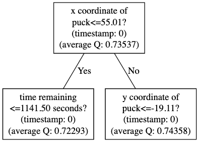
Figure 7. Rule Example 2 for Action-Value of Shots in Ice Hockey

4.3.4. Gaussian Mixture

This method uses the expectation maximization algorithm to calculate a two-component bivariate Gaussian mixture model (Dobra and Gehrke, 2002) for $(x_{i},y)$ data pairs.

$$p(x_{i},y)=\sum^{2}_{k=1}\pi_{k}\cdot\mathcal{N}(x_{i},y|\mu_{k},\Sigma_{k})$$

Then, the breakpoint $c_{i}$ that best separates the two Gaussian clusters on each predictor variable $x_{i}$ can be computed in closed form by quadratic discriminant analysis.

5. Evaluation

Here, we evaluate the mimic-learned models’ fidelity, that is, their ability to match the output of the black-box DRL model. We also rank features for predicting shot action-values and impacts by importance, then show rules that describe how the important features influence the predictions. All three of Sorting with Variance Reduction, Sorting with T-test and Iterative Segmented Regression are fast enough for scalable model tree learning, with Iterative Segmented Regression as the fastest method. Details on computational costs can be found in Figure 5.

5.1. Fidelity

A mimic model must show strong fidelity (Dancey et al., 2007), that is, the root mean squared difference (RMSE) between the prediction of the tree and the prediction of the DRL model must be small.

As Table  1 shows, Iterative Segmented Regression and Sorting with Variance Reduction achieve greater fidelity on test set than other methods. Given its speed (Figure 5), we recommend Iterative Segmented Regression as a good default method, and Sorting with Variance Reduction as a close second. The null model calculates the mean value of the response variable and uses that as its prediction. Table 4 reports high correlations between the outputs of the neural and mimic models: for iterative segmented regression, they are almost always above 0.9 and in many cases above 0.99.

5.2. Feature Importance

A basic question for understanding a neural net is which input features most influence its predictions. Given a model tree, we can compute the feature importance as the sum of variance reductions over all splits that use the feature (Liu and Schulte, 2018). Table 3 shows the feature importance of the top 10 most relevant features for the action-value of shots in ice hockey and soccer, with feature frequency defined as how many times the tree splits on the feature. Time remaining is important for both ice hockey and soccer because the probability of either team scoring another goal decreases quickly when not much time is left. Moreover, time remaining has a stronger influence on ice hockey than soccer because there are generally more goals in ice hockey. At the beginning of a game, the probability of a team scoring in ice hockey is higher than that in soccer. As time goes towards the end, the probability of scoring in ice hockey decreases more quickly than that in soccer. Unsurprisingly, puck/ball to goal distance and action outcomes (i.e. shots being blocked or not) are also among the most relevant features for shots in ice hockey and soccer.

Table 3. Top 10 Features for Shots

Ice Hockey	Feature Importance	Feature Frequency
time remaining ($t_{0}$)	0.0594	248
y coordinate of puck ($t_{0}$)	0.03418	228
x coordinate of puck ($t_{0}$)	0.02646	153
action blocked ($t_{0}$)	0.02016	12
manpower situation ($t_{0}$)	0.01203	14
home ($t_{0}$)	0.00629	1
angle between puck and goal ($t_{0}$)	0.00164	32
time remaining ($t_{-1}$)	0.00072	9
action: reception ($t_{-1}$)	0.00061	5
score differential ($t_{-1}$)	0.00026	23

Soccer	Feature Importance	Feature Frequency
action blocked ($t_{0}$)	0.01524	1
time remaining ($t_{0}$)	0.00711	36
distance to goal ($t_{0}$)	0.00144	31
action: through ball ($t_{-1}$)	0.00079	1
event duration ($t_{0}$)	0.00068	8
time remaining ($t_{-1}$)	0.00059	12
y velocity of ball ($t_{0}$)	0.00036	5
x coordinate of ball ($t_{0}$)	0.00015	28
manpower situation ($t_{0}$)	0.00011	1
action: cross ($t_{-1}$)	0.00011	2

5.3. Rule Extraction

We can extract rules that can be easily interpreted by humans from a model tree. The rules highlight relevant interactions among input features. They also expand on the feature importance by showing how the important features influence the predictions of the neural network.

For shots in ice hockey, Figure 6 is a part of a tree to demonstrate how rules can be extracted. First, how good a shot is for the home team is related to which team is taking possession of the puck. In other words, whether the shot is performed by the home team or the away team. By looking at the average Q-values of the corresponding child nodes, we see that it is better for the home team if they take a shot than if the away team takes a shot. If the shot is by the home team, its Q-values are related to the time remaining in the game: with little time left (less than 335 seconds), there is less of a chance of any team scoring. However, given sufficient time, the next feature the tree considers is whether the home team has a manpower advantage. Figure 7 shows another part of the same tree. It supports the rule that the action-value of shots in ice hockey is better when the puck is closer to the net (recall the defensive zone has negative x coordinates and offensive zone has positive x coordinates). If the puck is sufficiently close, then the tree next considers the y-coordinate of the puck location. Figure 8 is an excerpt from Figure 1 after a shot is blocked. It extracts the rule of impacts such that when a shot is blocked by the opposite team, the impact of the action is less bad when the puck is far from the net. If the puck is close to the net when the shot is blocked, a good opportunity to a goal is lost, therefore, the impact is much worse.

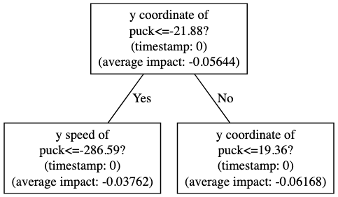
Figure 8. Rule Example for Impact of Shots in Ice Hockey

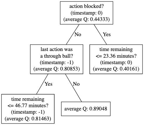
Figure 9. Rule Example for Action-Value of Shots in Soccer

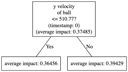
Figure 10. Rule Example for Impact of Shots in Soccer

For shots in soccer, Figure 9 is the top part of Figure 3. As in ice hockey, it shows that action-values of shots are better when shots are not blocked. Furthermore, it gives an insight that through-ball passes are not the best thing to do to assist a goal. The tree suggests that if a shot is taken right after a through-ball pass, the shot is usually less promising to a goal. For the impact of shots in soccer, Figure 10 presents a rule such that shots that are fast in y-direction usually have high impact values.

5.4. Debugging Deep Neural Networks

Because of the transparency of tree-based models, the tree learned from a DRL model can highlight potential problems in the DRL model. Figure 4 is part of a tree learned from an early version of a DRL Q-function model for ice hockey. The tree splits frequently on the feature Event Duration. When we presented the tree to ice hockey experts, the splits drew their attention - splitting frequently on duration conflicts with their expertise. As a consequence, we discovered an information leakage introduced in the data processing that extracted the duration feature, which caused it to highly correlate with Q-values. Without an interpretable model such as the tree, it is almost impossible to spot the spurious behaviour from the black box of the deep neural network.

6. Computational Feasibility

Several standard model tree learning packages failed to build on our large dataset due to their memory limitations. These include pyFIMTDD (Ikonomovska et al., 2011) and production systems such as Weka (at the University of Waikato, 2020) and GUIDE (Loh, 2020) that have been deployed in commercial applications. This highlights the need for new computational methods that can extend to large sports datasets.

All the experiments were performed on a computing node, provided by Compute Canada, with 4 core CPU and 64GB of RAM. Figure 5 shows the running time in hours for two actions, shots (150K events) and passes (1M events), for each breakpoint heuristic.

Iterative Segmented Regression is the fastest method. The sorting methods are slower but still bring the computational cost of the analysis to less than a day.

7. Conclusion and Future Work

The predictions of trained models must be explained if sports experts are to benefit fully from modern machine learning. Learning to mimic a neural net with a linear model tree offers a sweet spot in the accuracy-transparency trade-off: accurate predictions with rules and features that explicate the insights gained from data analysis. We introduced a new action replacement technique for augmenting sports data with soft labels from the neural network. Another new contribution are fast new heuristic methods for model tree construction that scale to large datasets. Mimic learning allows sports analytics to combine the predictive power of modern machine learning techniques with explanations and actionable insights for sports experts. A direction for future work is to investigate whether model trees support transfer learning between sports, as in our example of blocked shots. While specific threshold may be domain specific, trees can identify which combinations of features are important across sports.

Appendix A Dataset and Model Tree Construction

A.1. Predictive Variables in the Dataset

For ice hockey, we only considered regulation time for each game match and did not consider overtime periods (which are governed by substantially different rules).

A.2. Tree Construction

When describing tree learning algorithms, we use $x=(x_{1},x_{2},\dots,x_{m})$ for input features (covariates), and y for the output (dependent) variable. In our application, $x$ is a feature set for a state $S$, and $y=Q(S,A)$ is the output Q-value of the neural net for a fixed action $A$. The standard schema for growing a model tree is as follows (Breiman, 2017).

1. Initialization. Start with the root node. Assign all data records to it.

2. Growth Phase. At every leaf node $l$, for every input feature $x_{i}$, compute a promising breakpoint $c_{i}$.

   1. If no split $(x_{i},c_{i})$ improves the splitting criterion, keep $l$ as a leaf node.

   2. Otherwise find the split $(x_{i},c_{i})$ that maximizes the splitting criterion. Assign the data records for $l$ with $x_{i}\leq c_{i}$ to the left child of $l$, and those with $x_{i}>c_{i}$ to the right child of $l$.

3. Pruning Phase. Consider the parent $v$ of two leaf nodes $v_{1}$ and $v_{2}$. If the pruning criterion improves by replacing the two leaf nodes by $v$ as the leaf, prune the two leaf nodes.

A.3. Splitting Criterion

Following (Breiman, 2017), we split the tree at the point $(x_{i},c_{i})$ that gives the greatest reduction in y-variance, so the splitting criterion is:

$$\text{Variance}(s)-[\frac{N_{s_{t}}}{N_{s}}\cdot\text{Variance}(s_{t})+\frac{N_{s_{f}}}{N_{s}}\cdot\text{Variance}(s_{f})]$$

where $s$ is the whole set of data records $(x_{i})$ on a node, $s_{t}$ is the set of data records on a child node for which the split condition is true $(x_{i}\leq c_{i})$, $s_{f}$ is the set of data records on another child node for which the split condition is false $(x_{i}>c_{i})$, and $N_{s}$ represents the number of data records in set $s$.

A.4. Pruning the Tree

Growing a tree by variance reduction captures many informative interactions but tends to overfit. It is therefore necessary to add a pruning phase. The dual objectives of the pruning phase are to maximize the fidelity of the tree and reduce its complexity to increase interpretability. This trade-off can be expressed as a regularized linear regression with a complexity penalty on the weight parameters. For a tree node $v$, let $N_{v}$ be the number of data records assigned to $v$. The loss function at node $v$ is given by

$$E_{v}=\text{arg}\min_{w}\sum^{N_{v}}_{j=1}y_{j}-(w\cdot x_{j})+\lambda\cdot R(w)$$

A split at node $v$ is removed if doing so decreases the $E$ value for node $v$. For the complexity penalty R we use the L0-norm (number of parameters) or the L1-norm (ridge regression). In our experiments, the L0-norm gives a smaller tree and the L1-norm gives better fidelity on the held-out testing set. By increasing the trade-off parameter $\lambda$, the user can obtain a smaller tree but with less fidelity.

A.5. Pruning Criterion

For a tree node $v$, let $N_{v}$ be the number of data records assigned to $v$. Consider the parent $v$ of two leaf nodes $v_{1}$ and $v_{2}$. The pruning criterion is $E$, so if $E_{v}<E_{v1}+E_{v2}$, then we prune the two leaf nodes and make $v$ a new leaf node. Pruning is repeated until $E_{v}>=E_{v1}+E_{v2}$ for all leaf node parents $v$.

Table 4. Correlation Between Predictions of Model Tree and DRL Model

	Ice Hockey				Soccer
	Shots		Passes		Shots		Passes
Split methods	action-values	impacts	action-values	impacts	action-values	impacts	action-values	impacts
Gaussian Mixture	0.91498	0.93709	0.94737	0.91687	0.99458	0.99001	0.98386	0.81639
Iterative Segmented Regression	0.99436	0.93620	0.99601	0.92018	0.99650	0.99422	0.98695	0.81966
Sorting + Variance Reduction	0.99593	0.95834	0.99561	0.92137	0.99480	0.99459	0.98438	0.80024
Sorting + T-test	0.91036	0.89935	0.79761	0.85017	0.98943	0.98705	0.95690	0.79132
Null Model	0.00000	0.00000	0.00000	0.00000	0.00000	0.00000	0.00000	0.00000

References

- (1)
- Andras (2002) Peter Andras. 2002. The equivalence of support vector machine and regularization neural networks. Neural Processing Letters 15, 2 (2002), 97–104.
- at the University of Waikato (2020) Machine Learning Group at the University of Waikato. 2020. Weka. https://www.cs.waikato.ac.nz/ml/weka/
- Ba and Caruana (2014) Jimmy Ba and Rich Caruana. 2014. Do Deep Nets Really Need to be Deep?. In Advances in Neural Information Processing Systems 27: Annual Conference on Neural Information Processing Systems 2014, December 8-13 2014, Montreal, Quebec, Canada. 2654–2662.
- Biecek (2018) Przemyslaw Biecek. 2018. DALEX: Explainers for Complex Predictive Models in R. J. Mach. Learn. Res. 19 (2018), 84:1–84:5. http://jmlr.org/papers/v19/18-416.html
- Breiman (2017) Leo Breiman. 2017. Classification and regression trees. Routledge.
- Burke (2019) Brian Burke. 2019. DeepQB: deep learning with player tracking to quantify quarterback decision-making & performance. In Proceedings of the 2019 MIT Sloan Sports Analytics Conference.
- Cervone et al. (2014) Dan Cervone, Alexander D’Amour, Luke Bornn, and Kirk Goldsberry. 2014. POINTWISE: Predicting points and valuing decisions in real time with NBA optical tracking data. In Proceedings of the 8th MIT Sloan Sports Analytics Conference, Boston, MA, USA, Vol. 28. 3.
- Che et al. (2016) Zhengping Che, Sanjay Purushotham, Robinder G. Khemani, and Yan Liu. 2016. Interpretable Deep Models for ICU Outcome Prediction. In AMIA 2016, American Medical Informatics Association Annual Symposium, Chicago, IL, USA, November 12-16, 2016.
- Dancey et al. (2007) Darren Dancey, Zuhair Bandar, and David McLean. 2007. Logistic Model Tree Extraction From Artificial Neural Networks. IEEE Trans. Systems, Man, and Cybernetics, Part B 37, 4 (2007), 794–802. https://doi.org/10.1109/TSMCB.2007.895334
- Dobra and Gehrke (2002) Alin Dobra and Johannes Gehrke. 2002. SECRET: a scalable linear regression tree algorithm. In Proceedings of the eighth ACM SIGKDD international conference on Knowledge discovery and data mining. 481–487.
- Fernández et al. (2019) Javier Fernández, Luke Bornn, and Dan Cervone. 2019. Decomposing the immeasurable sport: A deep learning expected possession value framework for soccer. In 13th MIT Sloan Sports Analytics Conference.
- Guidotti et al. (2019) Riccardo Guidotti, Anna Monreale, Stan Matwin, and Dino Pedreschi. 2019. Black Box Explanation by Learning Image Exemplars in the Latent Feature Space. (2019).
- Ho (1995) Tin Kam Ho. 1995. Random decision forests. In Proceedings of 3rd international conference on document analysis and recognition, Vol. 1. IEEE, 278–282.
- Ikonomovska et al. (2011) Elena Ikonomovska, João Gama, and Sašo Džeroski. 2011. Learning model trees from evolving data streams. Data mining and knowledge discovery 23, 1 (2011), 128–168.
- Johansson et al. (2014) Ulf Johansson, Cecilia Sönströd, and Rikard König. 2014. Accurate and interpretable regression trees using oracle coaching. In 2014 IEEE Symposium on Computational Intelligence and Data Mining (CIDM). IEEE, 194–201.
- Lee (1992) Austin FS Lee. 1992. Optimal sample sizes determined by two–sample welch’s t test. Communications in Statistics-Simulation and Computation 21, 3 (1992), 689–696.
- Liu and Schulte (2018) Guiliang Liu and Oliver Schulte. 2018. Deep Reinforcement Learning in Ice Hockey for Context-Aware Player Evaluation. In Proceedings of the Twenty-Seventh International Joint Conference on Artificial Intelligence, IJCAI 2018, July 13-19, 2018, Stockholm, Sweden. 3442–3448.
- Loh (2020) Wei-Yin Loh. 2020. GUIDE Classification and Regression Trees and Forests. http://pages.stat.wisc.edu/~loh/guide.html
- Mitchell (1997) Tom M. Mitchell. 1997. Machine learning. McGraw-Hill. http://www.worldcat.org/oclc/61321007
- Muggeo (2003) Vito MR Muggeo. 2003. Estimating regression models with unknown break-points. Statistics in medicine 22, 19 (2003), 3055–3071.
- Rummery and Niranjan (1994) Gavin A Rummery and Mahesan Niranjan. 1994. On-line Q-learning using connectionist systems. Vol. 37. University of Cambridge, Department of Engineering Cambridge, UK.
- Schulte et al. (2017) Oliver Schulte, Zeyu Zhao, Mehrsan Javan, and Philippe Desaulniers. 2017. Apples-to-apples: Clustering and ranking NHL players using location information and scoring impact. In Proceedings of the MIT Sloan Sports Analytics Conference.
- Uther and Veloso (1998) William TB Uther and Manuela M Veloso. 1998. Tree based discretization for continuous state space reinforcement learning. In Aaai/iaai. 769–774.
- Vens and Blockeel (2006) Celine Vens and Hendrik Blockeel. 2006. A simple regression based heuristic for learning model trees. Intelligent Data Analysis 10, 3 (2006), 215–236.
- Wang et al. (2018) Jiaxuan Wang, Ian Fox, Jonathan Skaza, Nick Linck, Satinder Singh, and Jenna Wiens. 2018. The advantage of doubling: a deep reinforcement learning approach to studying the double team in the NBA. arXiv preprint arXiv:1803.02940 (2018).
- Yurko et al. (2019) Ronald Yurko, Samuel Ventura, and Maksim Horowitz. 2019. nflWAR: a reproducible method for offensive player evaluation in football. Journal of Quantitative Analysis in Sports 15, 3 (2019), 163–183.