EDropout: Energy-Based Dropout and Pruning of Deep Neural Networks

Abstract

Dropout is a well-known regularization method by sampling a sub-network from a larger deep neural network and training different sub-networks on different subsets of the data. Inspired by the dropout concept, we propose EDropout as an energy-based framework for pruning neural networks in classification tasks. In this approach, a set of binary pruning state vectors (population) represents a set of corresponding sub-networks from an arbitrary original neural network. An energy loss function assigns a scalar energy loss value to each pruning state. The energy-based model stochastically evolves the population to find states with lower energy loss. The best pruning state is then selected and applied to the original network. Similar to dropout, the kept weights are updated using backpropagation in a probabilistic model. The energy-based model again searches for better pruning states and the cycle continuous. This procedure is in fact a switching between the energy model, which manages the pruning states, and the probabilistic model, which updates the kept weights, in each iteration. The population can dynamically converge to a pruning state. This can be interpreted as dropout leading to pruning the network. From an implementation perspective, unlike most of the pruning methods, EDropout can prune neural networks without manually modifying the network architecture code. We have evaluated the proposed method on different flavours of ResNets, AlexNet, $l_{1}$ pruning, ThinNet, ChannelNet, and SqueezeNet on the Kuzushiji, Fashion, CIFAR-10, CIFAR-100, Flowers, and ImageNet datasets, and compared the pruning rate and classification performance of the models. The networks trained with EDropout on average achieved a pruning rate of more than $50\%$ of the trainable parameters with approximately $<5\%$ and $<1\%$ drop of Top-1 and Top-5 classification accuracy, respectively.

I Introduction

Deep neural networks (DNNs) have different learning capacities based on the number of trainable parameters for classification tasks. Depending on the complexity of the dataset (e.g. size of dataset and number of classes), selecting a network which maximizes the generalization performance often involves trial and error. A DNN with larger capacity often has better performance, but may suffer from a longer training time, lack of generalization, and redundancy in trained parameters. DNNs are computationally intensive, require large memory, and consume extensive energy [1]. Hence, smaller networks are more desirable for applications such as edge computing and embedded systems. Pruning DNNs is one of the major approaches for reducing the number of trainable parameters while maintaining the classification performance. Most of the proposed methods for deploying DNN on edge devices can be divided into pruning existing networks or small networks by design. Our focus in this paper is on methods that can prune a given DNN.

Dropout [2], which was originally proposed as a regularization technique to train DNNs, reduces complexity of the network by randomly dropping a subset of the parameters in each training phase but fully utilizing the parameters (full network) for inference. Despite other regularization methods such as $l_{1}$ and $l_{2}$ norms [3], which modify the loss function, the dropout-based methods modify the network structure, which is equivalent to training different smaller neural networks. A variety of methods has been proposed for smarter dropout such as standout [4], variational dropout [5], and adversarial dropout [6]. Dropout is mainly proposed for dense layers while it is much less used in convolution layers. While dropout [2] sets a subset of activation values to zero, DropConnect [7] zeroes a randomly selected subset of weights in a fully connected network. A survey on dropout methods is provided in [8].

Pruning is different from dropout, in which the trainable parameters are permanently dropped, and is mainly used to remove redundant weights while preserving the classification accuracy. Removing inactive and redundant weights from a network can lead to a smaller network which has a better generalization performance and a faster inference speed [9]. In general, pruning algorithms have three stages which are training, pruning, and fine-tuning [10]. One of the early attempts was to use second derivative information to minimize a cost function that reduces network complexity by removing excess number of trainable parameters and further training the remaining of the network to increase inference accuracy [9]. Soft weight-sharing [11] is another approach by clustering weights into subgroups with similar weight values. It adds a penalty term to the cost function of the network where the distribution of weight values is modeled as a mixture of multiple Gaussians and the means and variance of clusters are adapted during the training of network [11]. This work has been further enhanced in [12]. Deep Compression has three stages that are pruning, quantization, and Huffman coding, which targets reducing the storage requirement of a DNN without affecting its accuracy [1]. This method works by pruning all connections with weights below a threshold followed by retraining the sparsified network.

The concept of energy has also been used for pruning DNNs, where we have proposed an Ising energy-based model for dropout and pruning of hidden units in multi-layer perceptron (MLP) neural networks [13]. In this approach, the network is modeled as a graph where each node is a hidden unit and the edge between nodes represents a measure of activation of each unit. We used a high-speed hardware to search for the best sub-network using Markov Chain Monte-Carlo (MCMC) [14] method. Later, we scaled up this method for pruning large-scale MLPs using a node grouping technique [15] and pruning DCNNs [16].

Figure 1: Top: Unstructured pruning; Bottom: Structured pruning. Red elements are pruned.

In this paper, we introduce the concept of using energy-based models (EBMs) [17] for pruning of convolutional and dense layers. This method behaves as a hybrid technique, where similar to random dropout, it trains different sub-networks of the original DNN at a time, leading to a pruned network. The trained network is in fact a subset of the original network, which has a competitive performance to the network at full capacity but with a smaller number of parameters. We introduce utilizing a population of pruning candidate states, where each state vector in the population represents a set of active trainable weights from the network. Each vector has a corresponding energy loss value as a measure of dependency between sub-network parameters. The objective is to search for state vectors with lower energy loss. Indeed, for a DNN with $|\mathbf{\Theta}|$ number of trainable parameters, this is a combinatorial optimization problem which requires $2^{|\mathbf{\Theta}|}$ times evaluation of the energy loss function for each batch of data. Since this procedure is NP-hard, we also propose a stochastic parallel binary technique based on the differential evolution (DE) method [18], [19] to search for the sparse state of the network. In this paper, our focus is to study and evaluate EDropout in pruning DNNs and not as a regularization method. Our results show on average more than $50\%$ pruning of trainable network parameters while maintaining classification performance — the Top-1 and Top-5 classification accuracy drop on average $<5\%$ and $<1\%$, respectively — on several image classification tasks with various number of classes and available training samples on the ResNets, AlexNet, $l_{1}$ pruning, ThinNet, ChannelNet, and SqueezeNet.

Figure 2: Energy-based model (EBM), [17].

II Background

II-A Pruning Methods

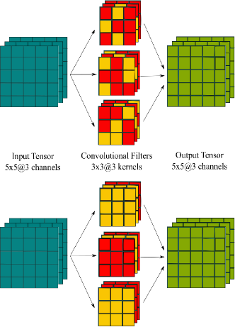
Pruning methods in neural networks can be divided into unstructured and structured methods. Figure 1 shows an illustration of these two approaches.

II-A1 Unstructured Pruning

Unstructured pruning removes any subset of weights without following a specific geometry like the entire kernel, filter, or channel [20]. This kind of pruning results in a sub-network with geometrically sparse weights, which is difficult to implement in practice as a smaller network due to predefined tensor-based operations on graphical processing units (GPUs). It also requires overhead computation to address the location of kept weights. Therefore, it is difficult to get computational advantage from this approach. However, due to granular level of sparsity, this approach generally has lower drop of accuracy compared with the structured methods and the original model.

II-A2 Structured Pruning

Structured pruning generally follows some constraints and defined structure in pruning a network. Typically pruning happens at channel, kernel, and intra-kernel levels. All the incoming and outgoing weights to/from a feature map are pruned in a channel level pruning which can result in an intensive reduction of network weights. In kernel level pruning, a subset of kernels is entirely pruned. Compared with the unstructured pruning, the structured pruning has very little computational cost overhead and is easier to implement and scale on GPUs. The advantage is faster implementation and inference. A group of state-of-the-art structured pruning algorithms is examined in [10], which concludes that fine-tuning a pruned model only gives comparable or worse performance than training the model with randomly initialized weights.

Figure 3: Different steps of the proposed combined optimization and training framework for pruning neural networks. Step 1: Population initialization; Step 2: Evolution of the population; Step 3: Compute energy loss value for each candidate state vector; Step 4: Select the state vector with the lowest energy loss value in the population; Step 5: Apply the state vector with lowest energy loss value (the best state vector) to the network; Step 6: Perform backpropagation (on the kept weights only); Step 7: Continue to step 2. $\mathbf{S}$: population of candidate pruning state vectors; $\mathbf{s}_{b}$: best pruning state vector; $\mathcal{E}_{s}$: energy loss of state vector $s$.

II-B Energy-based Models

In general, solving a classification problem using DNNs with $C$ data classes $\mathcal{Y}=\{y_{1},...,y_{C}\}$ is defined as using a parametric function to map the input $X\in\mathcal{X}$ to $C$ real-valued numbers $\epsilon=\{\varepsilon_{1},\varepsilon_{2},...,\varepsilon_{C}\}$ (a.k.a. logits). This function is in fact a stack of convolutional and dense layers with non-linear activation functions. The output is then passed to a classifier, such as Softmax function, which is a member of the Gibbs distributions, to parameterize a categorical distribution in form of a probability distribution over the data classes [21], defined as $\{p(y_{1}),...,p(y_{C})\}$ where for simplicity we define $p_{c}=p(y_{c})\>\forall\>c\in\{1,...,C\}$. The loss is then calculated based on cross-entropy with respect to the correct answer $Y$.

The Gibbs distribution (a.k.a the Boltzmann distribution), which is a very general family of probability distributions, is defined as

$$p(Y|X)=\frac{e^{-\beta\mathcal{F}(Y,X)}}{Z(\beta)},$$ (1)

where $Z(\beta)=\sum\limits_{y_{c}\in\mathcal{Y}}e^{-\beta\mathcal{F}(y_{c},X)}$ is the partition function, $\beta>0$ is the inverse temperature parameter [17], and $\mathcal{F}(\cdot)$ is referred to as Hamiltonian or the energy function. The Gibbs distribution naturally permits annealing, by changing the temperature during the training procedure [22]. $\beta$ is discussed in [23] as the distillation where a higher value for $1/\beta$ produces a softer probability distribution over classes.

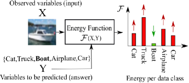
In general, some probabilistic models can be considered as a special type of EBMs. An EBM assigns a scalar energy loss as a measure of compatibility to a configuration of parameters in neural networks [17], as demonstrated in Figure 2. One of the advantages of this approach is avoiding normalization, which can be interpreted as an alternative to probabilistic estimation [17]. Calculating the exact probability in (1) needs computing the partition function over all the data classes $C$. However, for large $C$, such as in language models with more than $100,000$ classes, this causes a bottleneck [24]. In addition, in order to follow the probability axioms, specifically $\sum_{c=1}^{C}p_{c}=1$, the Softmax transfer function generates prior probability values that are close to zero for each class. Some methods such as annealed importance sampling [25] and negative sampling [26] have been proposed to facilitate computing of the partition function, which is out of the scope of this paper.

II-C Differential Evolution

Population-based optimization algorithms are popular methods for solving combinatorial high-dimensional optimization problems. The advantage of such methods is using a population of candidate solutions to search the problem landscape to minimize/maximize the objective function. DE [18] is one of the popular and well-known population based algorithms which has been used in different applications such as localization [27] and opposition-based learning [28]. The search procedure starts with $S$ initial candidate solutions (individuals) $\mathbf{S}^{S\times D}$ with dimension $D$ and based on the scaled difference between two selected individuals $\mathbf{s}_{i},\mathbf{s}_{j\neq i}\in\mathbf{S}$ improves the candidate solutions in each generation toward a feasible solution [19]. The standard version of DE for continuous problems has three major operations: mutation, crossover, and selection.

Mutation: For an individual $\mathbf{s}_{i}\in\mathbf{S}$, three different individuals $\mathbf{s}_{i_{1}}$, $\mathbf{s}_{i_{2}}$, and $\mathbf{s}_{i_{3}}$ are selected from $\mathbf{S}$. The mutant vector of $\mathbf{s}_{i}$ is then calculated as

$$\mathbf{v}_{i}=\mathbf{s}_{i_{1}}+F(\mathbf{s}_{i_{2}}-\mathbf{s}_{i_{3}}),$$ (2)

where the mutation factor $F\in(0.1,1.5)$ is a real constant that controls the amplification of the added differential variation of $\textbf{s}_{i_{2}}-\textbf{s}_{i_{3}}$. The exploration of DE increases by selecting higher values for $F$.

Crossover: The crossover operation increases diversity of the population by shuffling the mutant and parent vectors as

$$u_{i,d}=\left\{\begin{array}[]{ll}v_{i,d},&r^{\prime}_{d}\leq C_{r}\>\text{or}\>d_{rand}=d\\ s_{i,d},&\textrm{otherwise}\end{array},\right.$$ (3)

for all $d\in\{1,...,D\}$ and $i\in\{1,...,S\}$, where $C_{r}\in[0,1]$ is the crossover rate, $r^{\prime}_{d}\in[0,1]$, and $d_{rand}$ is a random integer from the interval $[1,D]$.

Selection: The $\mathbf{u}_{i}$ and $\mathbf{s}_{i}$ vectors are evaluated for each ${\mathbf{s}_{i}\in\mathbf{S}}$ and compared with respect to their fitness value. The one with better fitness (lower value for minimization problem) is selected for the next generation.

The above procedure generally continues for a predefined number of generations or until some convergence criteria are satisfied.

Figure 4: Switching between the energy-based model (EBM) and the probabilistic model. The EBM searches for the pruning state and the probabilistic models searches for the weights. Both models are aware of target class $Y$ during training. In inference, the best pruning state is applied and the EBM is removed.

III Energy-based Dropout and Pruning

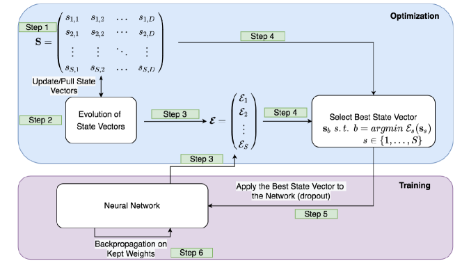
Figure 3 shows an overview of the proposed framework. It has two major phases which are optimization and training. The optimization phase manages searching for a state vector for dropout and ultimately pruning a neural network. The training phase trains a sub-network of the given neural network defined by the state vector suggested by the optimization phase. These two phases are conducted interchangeably in each iteration until an early state convergence condition (discussed in Subsection III-C4) is met. Then, the optimization phase is terminated and the training phased is focused on fine-tuning the sub-network, represented by the last suggested state vector. Details of these steps are discussed next.

III-A Pruning States

A given neural network has a set of trainable parameters $\mathbf{\Theta}$, which is generally a combination of parameters in convolutional and dense layers. In convolutional layers, we are interested in dropping weight filters (including bias terms) and in dense layers, the hidden units (including the bias terms and all incoming/outgoing connections). A feature map in a convolutional layer is the output of convolving a weight filter with the incoming activation values. Therefore, dropping a filter can also be interpreted as dropping a feature map or an input channel to the next layer.

Let us define a set of $S$ binary candidate pruning state vectors as the population $\mathbf{S}^{S\times D}$. Each vector $\mathbf{s}_{i}\in\mathbf{S}$ of length $D$ represents the state of trainable filters in a convolution layer and hidden units in the dense layers, referred to as a unit hereafter for convenience. If $s_{i,d}=0$ unit $d$ is dropped (inactive) and if $s_{i,d}=1$ it participates (active) during training and inference. Each state vector $\mathbf{s}_{i}$ corresponds to a sub-network of the original network with the corresponding energy function values $\mathcal{F}_{i}\in\{\mathcal{F}_{1},...,\mathcal{F}_{S}\}$, where generally we can have $2^{D}$ possible energy functions.

Figure 5: A simple convolutional neural network to visualize the energy landscape in Figure 6 with $2^{10}$ possible state vectors, where each state corresponds to a convolution filter.

Figure 6: Energy loss landscape for all possible pruning state vectors ($2^{10}$) during training iterations of the neural network in Figure 5.

III-B Energy Model

The Gibbs distribution gives considerable flexibility in defining pruning methods [22]. For example, every Markov random field (MRF) corresponds to a Gibbs distribution, and vice versa. Gibbs distribution is a probability measure to define the state of a system (such as a DNN) based on the given energy of the system. Softmax function which is the normalized exponential function generally used in training DNN for classification problems has the similar form as the Boltzmann distribution [29]. An energy function is a measure of compatibility, which represents the dependencies of a subset of the network variables as a scalar energy, based on the definition of EBMs in [17].

By choosing $\beta=1$ in the Gibbs distribution (1), the energy function corresponding to using a Softmax layer in training neural networks is given by

$$\mathcal{F}(Y,X)=-\epsilon,$$ (4)

where $\epsilon=(\varepsilon_{1},...,\varepsilon_{C})$. The Softmax function in training neural networks is defined as

$$p(y_{c}|X)=\frac{e^{\varepsilon_{c}}}{\sum_{\varepsilon_{c}\in\epsilon}e^{\varepsilon_{c}}}.$$ (5)

Since Softmax is a special case of the Gibbs distribution, by setting $\beta=1$ [29], and using the definition in (1) we have

$$p_{(}y_{c}|X)=\frac{e^{-\mathcal{F}(y_{c},X)}}{\sum_{y_{c}\in\mathcal{Y}}e^{-\mathcal{F}(y_{c},X)}},$$ (6)

where by comparing (1) and (6) we can interpret ${\mathcal{F}(y_{c},X)=-\varepsilon_{c}}$ and in a generalized form ${\mathcal{F}(Y,X)=-\epsilon}$ for all $\varepsilon_{c}\in\epsilon$.

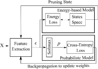
In EBMs, training a model refers to finding an energy function $\mathcal{F}(Y,X,\Theta)$ that minimizes the energy loss of the model by searching the weights space [17]. However, we define pruning as the searching for a binary state vector $\mathbf{s}$ that prunes the network while minimizes the energy loss for fixed $Y,X$, and $\Theta$ in each iteration, defined as $\mathcal{F}(Y,X,\Theta,\mathbf{s})$. We are using the cross-entropy loss and backpropagation to search for the weights. Hence, the search for weights is conducted using a probabilistic model when the pruning state vector is fixed and the search for pruning state is conducted using an EBM when the weights are fixed in each iteration, as illustrated in Figure 4. Based on this concept, the candidate state vectors discussed in Section III-A define different energy functions corresponding to different sub-networks of the original network. Evolution of the candidate state vectors in an energy minimization scheme helps to find a subset of the original network which corresponds to an energy function with low energy value.

We define the following energy loss function to measure the quality of an energy function for $(X,Y)$ with the target output $y_{c}$ as

$$\begin{split}\mathcal{E}&=\mathcal{L}(Y,\mathcal{F})\\ &=\mathcal{F}(y_{c},X)-min\{\mathcal{F}(y_{c^{\prime}},X):\;y_{c^{\prime}}\in\mathcal{Y},c^{\prime}\neq c\},\end{split}$$ (7)

where it can be extended for a batch of data. The energy loss function is intuitively designed to assign a low loss value to $\mathcal{F}_{s}$ which has the lowest energy with respect to the target data class $c$ and higher energy with respect to the other data classes and vice versa [17]. The corresponding energy loss values for the state vectors in Figure 3 are calculated in Step 3 as $\mathcal{E}=(\mathcal{E}_{1},...,\mathcal{E}_{S})$.

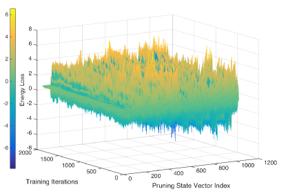
For sake of visualization, Figure 5 shows a simple neural network for an image classification task, which has $4$ filters in the first convolution layer and $6$ filters in the second convolution layer. For simplicity, we only focus on pruning the convolution filters. Hence, the length of a state vector $\mathbf{s}$ is $D=10$ such that $s_{d}\in\{0,1\}$. Figure 6 shows the complexity of the energy loss landscape of this network for all possible state vectors (i.e. $2^{D}=2^{10}$) over the training iterations, which shows finding a state vector with minimum energy loss value is a very complex NP-hard combinatorial problem with many possible local minima. In the next subsection, we discuss our proposed optimization approach to search for the best state vector on the energy landscape.

Set t = 0 // Optimization counter

Initiate the neural network with trainable weights $\Theta$

Set $\mathbf{S}^{(0)}\sim Bernoulli(P=0.5)$ // States initialization

Set $\Delta\mathbf{s}\neq 0$ & $\Delta\mathbf{s}_{T}$

for  $\mathit{i_{epoch}}=1\rightarrow\mathit{N_{epoch}}$ do // epoch counter

    for  $\mathit{i_{batch}}=1\rightarrow\mathit{N_{batch}}$ do // batch counter

         t = t+1

         if $\Delta\mathbf{s}\neq 0$ or $i_{epoch}\leq\Delta\mathbf{s}_{T}$ then

             if $i_{epoch}=1\;\&\;i_{batch}=1$ then

                 Compute energy loss of $\mathbf{S}^{(0)}$ as $\mathcal{E}^{(0)}$ using (7)

             end if

             for $i=1\rightarrow S$ do // States counter

                 Generate mutually different $i_{1},i_{2},i_{3}\in\{1,...,S\}$

                 for $d=1\rightarrow D$ do // State dimension counter

                     Generate a random number $r_{d}\in[0,1]$

                     Compute mutation vector $v_{i,d}$ using (8)

                 end for

                 Select candidate state $\tilde{s}^{(t)}_{i}$ using (9)

             end for

             Compute energy loss of $\tilde{\mathbf{S}}^{(t)}$ as $\tilde{\mathcal{E}}^{(t)}$ using (7)

             Select $\mathbf{S}^{(t)}$ and corresponding energy $\mathcal{E}^{(t)}$ using (10)

             Select the state with the lowest energy from $\mathbf{S}^{(t)}$ as $\mathbf{s}^{(t)}_{b}$

         else

             $\mathbf{s}^{(t)}_{b}=\mathbf{s}^{(t-1)}_{b}$

         end if

         Temporarily drop weights of the network based on the best state $\mathbf{s}^{(t)}_{b}$

         Compute loss of the sparsified network

         Perform backpropagation to update $\Theta$

    end for

    Update $\Delta\mathbf{s}$ for early state convergence using (11)

end for

Algorithm 1 EDropout

III-C Training and Optimization

Training and optimization in EDropout have the following major steps which are initialization, energy loss computation, energy loss optimization, early state convergence check, and training the sub-network in each iteration using backpropagation, as presented in Algorithm 1.

III-C1 Initialization

At the beginning of training ($t=0$), we initialize the candidate pruning states $\mathbf{S}^{(0)}\in\mathbb{Z}_{2}^{S\times D}$, where $s_{i,d}^{(0)}\sim Bernoulli(P=0.5)$ for $i\in\{1,...,S\}$ and $d\in\{1,...,D\}$.

III-C2 Computing Energy Loss

For each candidate state $\mathbf{s}_{i}^{(t)}\in\mathbf{S}^{(t)}$ in iteration $t$, the energy loss value is calculated using (7) as $\mathcal{E}^{(t)}_{i}$.

III-C3 Energy Loss Optimization

Searching for the pruning state which can minimize the energy loss value is an NP-hard combinatorial problem. Various methods such as MCMC and simulated annealing (SA) can be used to search for low energy states. We propose using a binary version of DE (BDE) [18] to minimize the energy loss function. This method has the advantage of searching the optimization landscape in parallel and sharing the search experience among candidate states. The other advantage of this approach is flexibility of designing the energy function with constraints.

a $F=0.1$

b $F=0.1$

c $F=0.9$

d $F=0.9$

e $F\in[0,1]$

f $F\in[0,1]$

Figure 7: Left: Visualization of mutated state vectors diversity in a single run. Right: Monte-Carlo simulation of mutated state vectors diversity for 1,000 runs.

The optimization step has three phases which are mutation, crossover, and selection. Given the population of states $\mathbf{S}^{(t-1)}$, a mutation vector is defined for each candidate state ${\mathbf{s}_{i}^{(t-1)}\in\mathbf{S}^{(t-1)}}$ as

$$v_{i,d}=\begin{cases}1-s_{i_{1},d}^{(t-1)},\>\>\>\>$if$\>\>\>s_{i_{2},d}^{(t-1)}\neq s_{i_{3},d}^{(t-1)}\;$\&$\;r_{d}<F\\ s_{i_{1},d}^{(t-1)},\>\>\>\>\>\>\>\>\>\>\>$ otherwise $\end{cases},$$ (8)

for all $d\in\{1,..,D\}$, where $i_{1},i_{2},i_{3}\in\{1,...,S\}$ are mutually different, $F$ is the mutation factor [19], and $r_{d}\in[0,1]$ is a random number. The next step is to crossover the mutation vectors to generate new candidate state vectors as

$$\tilde{s}^{(t)}_{i,d}=\begin{cases}v_{i,d}\>\>\>\>\>\>\>\>\>\>\>\>$if$\>\>\>r^{\prime}_{d}\in[0,1]\leq C_{r}\\ s_{i,d}^{(t-1)}\>\>\>\>\>\>\>\>\>\>\>$ otherwise $\end{cases},$$ (9)

where $C_{r}$ is the crossover coefficient [19]. The parameters $C_{r}$ and $F$ control exploration and exploitation of the population on the optimization landscape. Each generated state $\tilde{\mathbf{s}}_{i}^{(t)}$ is then compared with its corresponding parent with respect to its energy loss value $\tilde{\mathcal{E}}^{(t)}_{i}$ as

$$\mathbf{s}_{i}^{(t)}=\begin{cases}\tilde{\mathbf{s}}_{i}^{(t)}\>\>\>\>\>\>\>\>\>\>$if$\>\>\>\tilde{\mathcal{E}}^{(t)}_{i}\leq\mathcal{E}^{(t-1)}_{i}\\ \mathbf{s}_{i}^{(t-1)}\>\>\>\>\>$ otherwise $\end{cases}\>\forall\>i\in\{1,...,S\}.$$ (10)

The state with minimum energy loss $\mathcal{E}_{b}^{(t)}=min\{\mathcal{E}_{1}^{(t)},...,\mathcal{E}_{S}^{(t)}\}$ is selected as the best state $\mathbf{s}_{b}$, which represents the sub-network for next training batch. This optimization strategy is simple and feasible to implement in parallel for a large $S$. A predefined number of active states can be defined in the optimizer to enforce a specific dropout/pruning rate.

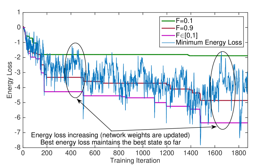
To better understand the importance of mutation factor, we select the energy loss landscape at iteration 1200 from Figure 6, where the state vector with the lowest energy loss is ${(1,1,1,1,0,0,0,1,1,1)}$ at index $968$ with an energy loss value of $-3.4715$. Then $S=8$ random state vectors are initialized, as illustrated by red markers in Figures 7(a), 7(c), and 7(e) for $F=0.1$, $F=0.9$, and $F\in[0,1]$, respectively, and $C_{r}=0.9$. Then, the state vectors are mutated only once, their energy loss is compared with their parent, and the state vector with lower energy loss is denoted by green markers. The plots show $F=0.9$ results in more diversity of mutated state vectors than $F=0.1$. We need to note that some mutated individuals may overlap, as observed for $F=0.1$ and $F=0.9$. If we use a random $F\in[0,1]$, the diversity is further enhanced compared to when using a constant $F$, and mutated states are more likely to have a lower energy loss value than their parent. In another visualization, we perform a Monte-Carlo simulation of the above experiment with 1,000 independent runs. Comparing Figures 7(b), 7(d), and 7(f) show that $F\in[0,1]$ has more exploration capability. In fact, for $F=0.1$, $F=0.9$, and $F\in[0,1]$, about $23.05\%$, $36.91\%$, and $60.35\%$ of the possible states are visited, respectively.

We also look at the energy loss landscape from the training iterations perspective. As Figure 8(a) shows, using the random $F\in[0,1]$ results in a better exploration of the optimization landscape, and ultimately, lower energy loss over the training iterations. It is interesting to observe that although the minimum energy loss value of a single input fluctuates during training (due to backpropagation on all training samples), the energy loss of selected state vectors remains the lowest possible for each iteration and enforces pruning while decreasing the overall energy loss.

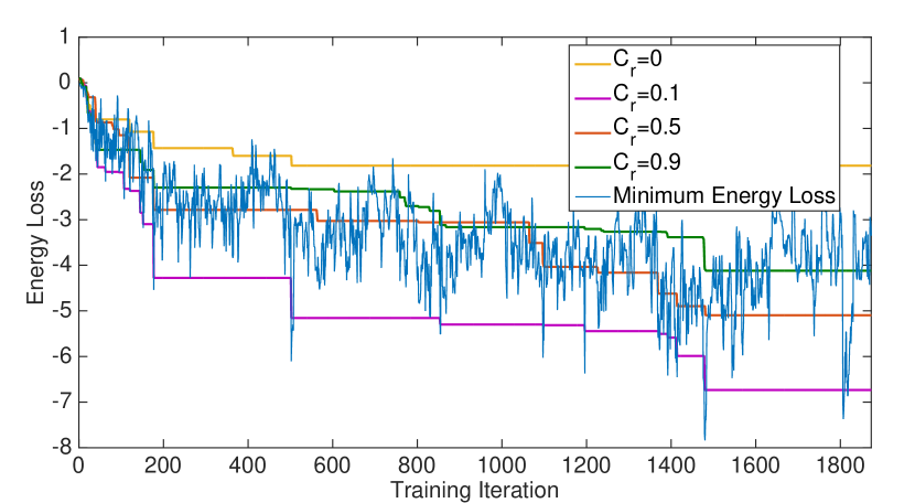
The last visualization is about the importance of the crossover rate, as illustrated in Figure 8(b) for $F\in[0,1]$. We can observe that the combination of the mutation factor and the crossover rate can control the exploration and exploitation of the search. Too much diversity ($F\in[0,1]$ and $C_{r}=0.9$) results in stagnation while a balance of these two parameters ($F\in[0,1]$ and $C_{r}=0.1$), can result in finding the states with lower energy loss.

a Convergence of best mutated state vector for different mutation factors with ${C_{r}=0.5}$.

b Convergence of best mutated state vector for different crossover rates with ${F\in[0,1]}$.

Figure 8: Convergence of best mutated state vector for different mutation factors and crossover rates.

III-C4 Early State Convergence

The population-based optimizers are global optimization methods which generally converge to a locally optimal solution. These algorithms suffer from premature convergence and stagnation problems [30]. The former generally occurs when the population (candidate state vectors) has converged to local optima, has lost its diversity, or has no improvement in finding better solutions. The latter happens mainly when the population remains diverse during training [30].

The optimization process can run for every iterations of the neural network training. However, after a number of iterations, depending on the capacity of the neural network and the complexity of the dataset, all the states in $\mathbf{S}^{(t)}$ may converge to a state $\mathbf{s}_{b}\in\mathbf{S}^{(t)}$. We call this the early state convergence phase and define it as

$$\Delta\mathbf{s}=\mathcal{E}_{b}^{(t)}-\frac{1}{S}\sum\limits_{j=1}^{S}\mathcal{E}_{j}^{(t)},$$ (11)

where $\mathcal{E}_{b}^{(t)}$ is the energy loss of $\mathbf{s}_{b}$. So, if $\Delta\mathbf{s}=0$ we can call for an early state convergence and continue training by fine-tuning the sub-network identified by the state vector $\mathbf{s}_{b}$. In addition, a stagnation threshold $\Delta\mathbf{s}_{T}$ is implemented where if $\Delta\mathbf{s}\neq 0$ after $\Delta\mathbf{s}_{T}$ number of training epochs, it stops the energy loss optimizer. These mechanisms are implemented to balance exploration and exploitation of the optimizer and address potential stagnation and premature convergence scenarios during training, as analyzed in Section IV-D1.

Most pruning and compression models first prune and train the network and then fine-tune it. The convergence to the best state $\mathbf{s}_{b}$ in EDropout breaks the training procedure of the neural network into two phases. The first phase is when various subsets of the neural network, with potential overlap of units, are trained, which occurs before the convergence, and the second phase is when only a subset of network, chosen by $\mathbf{s}_{b}$, is fine-tuned. The first phase is equivalent to training a network with dropout, which may act as a regularization method, and the second phase acts as fine-tuning where the pruned units/filters are not trained anymore and are practically eliminated from the network. This leads to a sparsified neural network. Training the sparsified network is similar to a typical training of DNNs with backpropagation.

III-C5 Training

Once the best candidate state is selected in each iteration, the state vector is applied to the network to compute the training loss. The backpropagation is then performed for the active units.

a Kept parameters

b Validation Loss

c Energy loss difference

d Best energy loss

e Validation energy loss

Figure 9: Convergence of ResNet-18 on Flowers validation dataset with $S=8$ and initialization probability of $P=0.5$ over 200 epochs.

a Rate of kept parameters

b Best energy loss

Figure 10: Number of candidate state vectors analysis of EDropout for ResNet-18 and Flowers dataset.

c Rate of kept parameters

d Best energy loss

Figure 11: States initialization analysis of EDropout for ResNet-18 and Flowers dataset.

IV Experiments

We have performed extensive experiments on datasets with different level of difficulty and number of samples on several DNNs with different capacities. First, we analyze the parameters of the EDropout method and then discuss the performance results.

IV-A Data

The following benchmark datasets are used: (i) Fashion (gray images in 10 classes, 54k train, 6k validation, and 10k test) [31], (ii) Kuzushiji (gray images in 10 classes, 54k train, 6k validation, and 10k test) [32]; (iii) CIFAR-10 (color images in 10 classes, 45k train, 5k validation, and 10k test) [33], (iv) CIFAR-100 (color images in 100 classes, 45k train, 5k validation, and 10k test) [33], (v) Flowers (102 flower categories; each class has between 40 and 258 images; 10 images from each class for validation and 10 for test) [34], and (vi) ImageNet (color images in 1,000 classes; the training and test datasets are standard from the other implementations) [35]. The horizontal flip and Cutout [36] augmentation methods are used for training on CIFAR and Flowers datasets. Input images are resized to $32\times 32$ for ResNets, $224\times 224$ for AlexNet [37] and SqueezeNet-v1.1 [38]. The input images for all models is of size $224\times 224$ for the ImageNet dataset [35].

IV-B Models

The experiments are conducted using the following models:

• ResNets (18, 34, 50, and 101 layers) [39].

• AlexNet [37], which is computationally very expensive.

• SqueezeNet v1.1 [38], which is a slim design of AlexNet.

• Deep Compression [1], which is a pruning and compression method.

• $l_{1}$ norm [40] pruning method. It has two versions A and B, where the first has a filter pruning rate of $\approx 10\%$ and skips the sensitive layers 16, 20, 38 and 54 in ResNet-56. The later has a combination three pruning rates for different layers ($60\%$, $30\%$ and $10\%$) and skips layers 16, 18, 20, 34, 38, and 54, [40]. We used version A mainly implemented for ResNet-34 for the ImageNet dataset.

• ThiNet [41], which is a filter level pruning method. We use the implementation provided for ResNet-50.

• ChannelNet [42], which is a slim network by design. It has three versions and we use ChannelNet-v2 which has the highest Top-1 accuracy [42] on the ImageNet dataset [35]. It also has better performance than MobileNet [43] as reported in [35].

IV-C Training Setup

The results are averaged over five independent runs. A grid hyper-parameter search is conducted based on the Top-1 accuracy for all models, including initial learning rates in $\{0.01,0.1,1\}$, Stochastic Gradient Descent (SGD) and Adadelta [44] optimizer, exponential and step learning rate decays with gamma values in $\{25,50\}$ and batch sizes of 64 and 128. The Adadelta optimizer with Step adaptive learning rate (step: every 50 epochs at gamma rate of 0.1) and weight decay of $10e^{-6}$ is used. The number of epochs is 200 and the batch size is set to 128. Random dropout is not used in the EDropout experiments. For the other models, where applicable, the random dropout rate is set to 0.5. The early state convergence in (11) is used with a threshold of 100 epochs. The models are implemented in PyTorch and trained using three NVIDIA Titan RTX GPUs.

IV-D Exploration vs. Exploitation: Dropout Leading to Pruning

The balance between exploration and exploitation in searching for the best state vector is crucial. The number of candidate state vectors, initialization of the states, mutation factor, and cross-over rate are among the major parameters to control diversity of search.

TABLE I: Performance study of ResNet-18 on the Flowers dataset for different early state convergence thresholds $\Delta\mathbf{s}_{T}$.

$\Delta\mathbf{s}_{T}$ Loss Top-1 Top-3 Top-5 $R$ 50 1.7867 55.55 77.59 83.78 48.04 100 1.6550 61.54 79.18 85.55 48.19 150 1.8088 55.55 74.86 82.12 48.78 200 1.6853 57.31 75.73 82.89 46.72

TABLE II: Performance study of ResNet-18 on the Flowers dataset for different number of candidate states $S$.

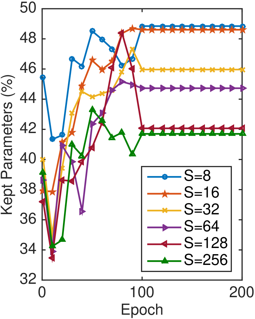
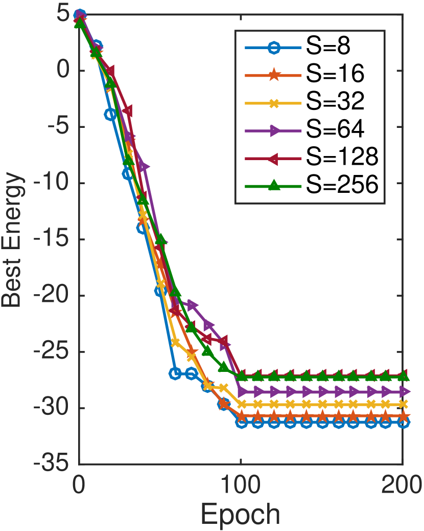
$S$ Loss Top-1 Top-3 Top-5 $R$ 8 1.6550 61.54 79.18 85.55 48.19 16 1.8029 55.93 75.74 81.92 48.60 32 1.7523 56.45 76.43 82.91 45.96 64 1.7248 57.20 77.69 83.97 44.72 128 1.7163 57.50 76.72 82.80 42.06 256 1.7042 58.12 77.62 83.69 41.69

TABLE III: Performance study of ResNet-18 on the Flowers dataset for different states initialization probability $P$.

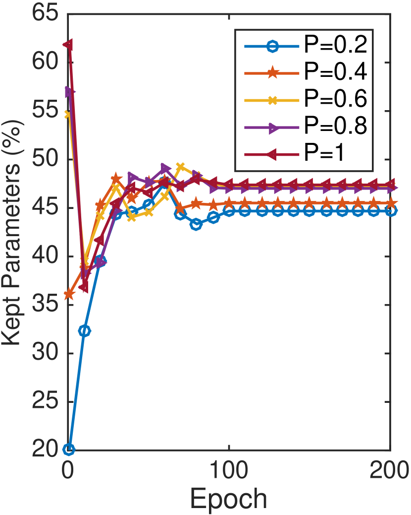
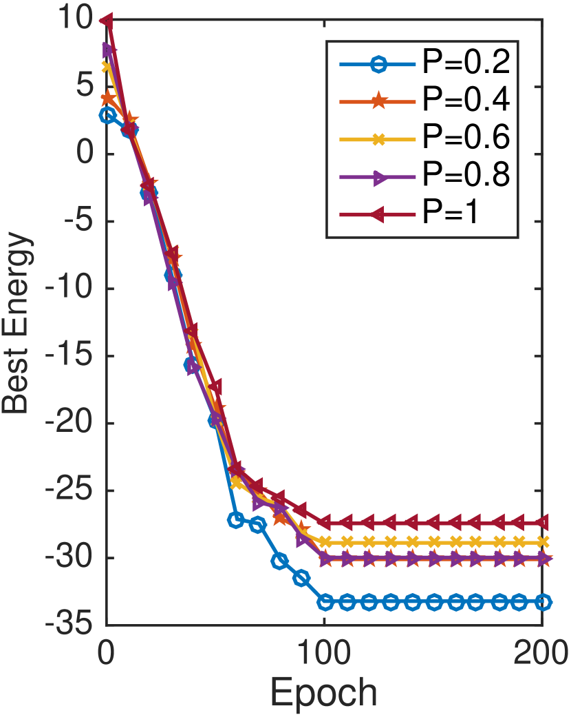
$P$ Loss Top-1 Top-3 Top-5 $R$ 0.2 1.6905 60.45 78.51 84.58 44.68 0.4 1.6776 59.39 77.60 83.80 46.25 0.6 1.7209 59.38 77.42 83.40 47.19 0.8 1.7084 58.97 77.70 83.97 47.31 1 1.6401 59.66 78.01 84.58 47.38

TABLE IV: Classification performance of ResNets [39], Deep Compression (DC) [1], $l_{1}$ norm [40], and ThiNet [45] on the test datasets. $R$ is kept trainable parameters and $\#p$ is approximate number of trainable parameters. All the values except loss and $\#p$ are in percentage. (F) refers to full network and (P) refers to pruned network used for inference with EDropout.

(a) Kuzushiji

Model Loss Top-1 Top-3 Top-5 $R$ $\#p$ ResNet-18 0.0709 98.23 99.53 99.79 100 11.1M ResNet-18+DC 0.1617 95.92 98.91 99.58 51.49 5.7M ResNet-18+EDropout(F) 0.1112 97.75 99.41 99.78 100 11.1M ResNet-18+EDropout(P) 0.1107 97.78 99.45 99.73 51.49 5.7M ResNet-34 0.0704 99.52 99.90 99.93 100 21.2M ResNet-34+$l_{1}$ norm 0.1054 98.50 99.02 99.89 90.65 19.2M ResNet-34+DC 0.2023 94.42 98.66 99.55 46.11 9.8M ResNet-34+EDropout(F) 0.1115 97.78 99.42 99.72 100 21.2M ResNet-34+EDropout(P) 0.1143 97.71 99.44 99.65 46.11 9.8M ResNet-50 0.0902 97.70 99.44 99.79 100 23.5M ResNet-50+ThiNet 0.2278 95.74 97.41 99.50 44.04 10.3M ResNet-50+DC 0.2142 94.36 98.53 99.36 45.57 10.7M ResNet-50+EDropout(F) 0.1250 97.89 99.38 99.75 100 23.5M ResNet-50+EDropout(P) 0.1289 97.63 99.35 99.73 45.57 10.7M ResNet-101 0.0699 98.26 99.63 99.80 100 42.5M ResNet-101+DC 0.5648 93.30 98.48 99.39 46.00 19.5M ResNet-101+EDropout(F) 0.1140 98.06 99.39 99.69 100 42.5M ResNet-101+EDropout(P) 0.1087 98.05 99.47 99.69 46.00 19.5M

(b) Fashion

Model Loss Top-1 Top-3 Top-5 R $\#p$ ResNet-18 0.2786 93.87 99.39 99.68 100 11.1M ResNet-18+DC 0.2299 91.97 99.32 99.86 50.43 5.6M ResNet-18+EDropout(F) 0.4000 93.45 99.04 99.47 100 11.1M ResNet-18+EDropout(P) 0.3934 93.57 99.06 99.47 50.43 5.6M ResNet-34 0.3198 93.61 99.12 99.62 100 21.2M ResNet-34+$l_{1}$ norm 0.3742 91.60 97.49 98.76 90.65 19.2M ResNet-34+DC 0.2632 90.62 99.26 99.87 46.94 9.9M ResNet-34+EDropout(F) 0.4674 92.80 98.78 99.35 100 21.2M ResNet-34+EDropout(P) 0.4582 92.57 98.68 99.35 46.94 9.9M ResNet-50 0.3187 93.34 99.15 99.60 100 23.5M ResNet-50+ThiNet 0.3052 92.19 97.93 98.83 44.04 10.3M ResNet-50+DC 0.2956 89.22 98.95 99.79 45.14 10.6M ResNet-50+EDropout(F) 0.5451 92.91 98.70 99.34 100 23.5M ResNet-50+EDropout(P) 0.5154 92.97 98.79 99.33 45.14 10.6M ResNet-101 0.3208 93.31 99.10 99.63 100 42.5M ResNet-101+DC 1.4812 89.94 98.72 99.46 45.19 19.2M ResNet-101+EDropout(F) 0.5785 92.58 98.83 99.40 100 42.5M ResNet-101+EDropout(P) 0.5717 92.57 98.82 99.35 45.19 19.2M

(c) CIFAR-10

Model Loss Top-1 Top-3 Top-5 $R$ $\#p$ ResNet-18 0.3181 92.81 98.78 99.49 100 11.2M ResNet-18+DC 0.6951 76.15 94.16 98.59 49.66 5.5M ResNet-18+EDropout(F) 0.4906 90.96 98.33 99.60 100 11.2M ResNet-18+EDropout(P) 0.4745 90.96 98.40 99.58 49.66 5.5M ResNet-34 0.3684 92.80 98.85 99.71 100 21.3M ResNet-34+$l_{1}$ norm 0.3888 90.63 97.14 99.25 90.65 19.3M ResNet-34+DC 1.0570 66.51 91.40 97.68 38.83 8.3M ResNet-34+EDropou(F) 0.4576 88.28 97.47 99.31 100 21.3M ResNet-34+EDropout(P) 0.4598 88.21 97.48 99.28 38.83 8.3M ResNet-50 0.3761 92.21 98.70 99.51 100 23.5M ResNet-50+ThiNet 1.0239 79.83 95.52 98.38 43.82 10.3M ResNet-50+DC 1.0271 67.53 89.92 96.30 46.39 10.9M ResNet-50+EDropout(F) 0.6041 85.22 96.35 98.77 100 23.5M ResNet-50+EDropout(P) 0.5953 85.30 96.62 98.76 46.39 10.9M ResNet-101 0.3680 92.66 98.69 99.65 100 42.5M ResNet-101+DC 1.037 66.32 92.65 98.11 45.10 19.2M ResNet-101+EDropout(F) 0.6231 86.97 97.42 99.24 100 42.5M ResNet-101+EDropout(P) 0.6339 86.57 97.37 99.20 45.10 19.2M

(d) CIFAR-100

Model Loss Top-1 Top-3 Top-5 $R$ $\#p$ ResNet-18 1.3830 69.03 84.44 88.90 100 11.2M ResNet-18+DC 2.3072 40.01 62.20 72.28 48.04 5.4M ResNet-18+EDropout(F) 1.9479 67.04 84.11 89.43 100 11.2M ResNet-18+EDropout(P) 1.9541 67.06 84.14 89.27 48.04 5.4M ResNet-34 1.3931 69.96 85.65 90.10 100 21.3M ResNet-34+$l_{1}$ norm 1.7033 68.12 81.32 84.73 90.65 19.3M ResNet-34+DC 2.1778 42.09 65.01 74.31 49.41 10.5M ResNet-34+EDropout(F) 1.9051 64.50 81.38 86.87 100 21.3M ResNet-34+EDropout(P) 1.9219 64.79 81.28 86.74 49.41 10.5M ResNet-50 1.3068 71.22 86.47 90.74 100 23.7M ResNet-50+ThiNet 2.0835 53.61 75.25 79.73 44.30 10.5M ResNet-50+DC 2.3115 43.87 67.02 76.26 46.01 10.9M ResNet-50+EDropout(F) 1.8750 61.60 79.52 85.45 100 23.7M ResNet-50+EDropout(P) 1.8768 61.91 79.99 85.87 46.01 10.9M ResNet-101 1.3574 71.19 85.54 90.00 100 42.6M ResNet-101+DC 2.6003 37.08 58.78 68.76 43.76 18.6M ResNet-101+EDropout(F) 1.9558 61.52 79.71 85.20 100 42.6M ResNet-101+EDropout(P) 1.9412 61.92 79.49 85.23 43.76 18.6M

(e) Flowers

Model Loss Top-1 Top-3 Top-5 $R$ $\#p$ ResNet-18 1.8262 62.60 80.64 86.92 100 11.2M ResNet-18+DC 2.4988 53.92 60.68 76.38 48.19 5.4M ResNet-18+EDropout(F) 1.6808 58.73 77.19 82.40 100 11.2M ResNet-18+EDropout(P) 1.6550 61.54 79.18 85.55 48.19 5.4M ResNet-34 1.8993 63.22 81.08 87.16 100 21.3M ResNet-34+$l_{1}$ norm 1.9935 60.23 83.42 85.36 90.65 19.3M ResNet-34+DC 2.4240 52.55 77.54 81.46 42.79 9.1M ResNet-34+EDropout(F) 1.6088 63.96 79.95 85.64 100 21.3M ResNet-34+EDropout(P) 1.5960 64.19 80.19 85.58 42.79 9.1M ResNet-50 2.4766 63.75 80.24 87.21 100 23.7M ResNet-50+ThiNet 2.3883 41.76 66.29 72.41 44.30 10.5M ResNet-50+DC 3.0556 27.28 47.43 57.63 44.68 10.6M ResNet-50+EDropout(F) 1.8492 54.60 76.46 82.84 100 23.7M ResNet-50+EDropout(P) 1.8293 56.02 76.42 83.10 44.68 10.6M ResNet-101 2.6183 62.70 82.04 86.26 100 42.7M ResNet-101+DC 3.0623 28.36 46.78 56.32 44.85 19.2M ResNet-101+EDropout(F) 1.8241 59.44 79.02 85.67 100 42.7M ResNet-101+EDropout(P) 1.8575 58.17 78.32 85.10 44.85 19.2M

(f) ImageNet

Model Loss Top-1 Top-3 Top-5 $R$ $\#p$ ResNet-18 1.9033 68.48 81.84 89.01 100 11.5M ResNet-18+DC 2.4053 55.03 70.23 77.14 46.27 5.3M ResNet-18+EDropout(F) 1.8503 64.95 82.23 87.16 100 11.5M ResNet-18+EDropout(P) 1.8550 65.43 82.53 87.26 46.27 5.3M ResNet-34 1.4921 73.42 85.93 91.26 100 21.6M ResNet-34+$l_{1}$ norm 1.5294 72.42 87.29 90.83 89.35 19.3M ResNet-34+DC 1.9606 63.71 81.15 88.03 44.06 9.5M ResNet-34+EDropout(F) 1.4148 71.39 86.93 90.27 100 21.6M ResNet-34+EDropout(P) 1.3996 71.82 87.20 90.96 44.06 9.5M ResNet-50 1.1959 75.27 87.48 91.87 100 24M ResNet-50+ThiNet 1.2303 72.11 86.30 90.37 51.66 12.4M ResNet-50+DC 2.0390 67.02 83.53 86.67 42.74 10.2M ResNet-50+EDropout(F) 1.1905 73.06 87.09 90.19 100 24M ResNet-50+EDropout(P) 1.0502 73.72 88.21 91.21 42.74 10.2M ResNet-101 1.5821 75.94 86.34 92.41 100 43M ResNet-101+DC 2.1014 64.62 79.28 85.24 42.94 18.46M ResNet-101+EDropout(F) 1.6391 72.52 85.33 91.21 100 43M ResNet-101+EDropout(P) 1.5519 73.94 87.34 92.08 42.94 18.46M

TABLE V: Classification performance of ChannelNet [42], AlexNet [37], and SqueezeNet [38] on the test datasets. $R$ is kept trainable parameters and $\#p$ is approximate number of trainable parameters. All the values except loss and $\#p$ are in percentage. (F) refers to full network used for inference and (P) refers to pruned network using EDropout. ChannelNet and SqueezeNet are compact models, which is a different approach from pruning.

(a) Kuzushiji

Model Loss Top-1 Top-3 Top-5 $R$ $\#p$ ChannelNet-v2 0.0788 98.15 99.56 99.89 100 1.8M AlexNet 0.1162 97.77 99.43 99.85 100 57M AlexNet+EDropout(F) 0.1976 96.53 99.25 99.72 100 57M AlexNet+EDropout(P) 0.2089 96.57 99.24 99.68 78.57 44.8M SqueezeNet 0.2114 97.19 99.27 99.72 100 0.72M SqueezeNet+EDropout(F) 0.2414 96.45 99.05 99.57 100 0.72M SqueezeNet+EDropout(P) 0.2411 96.35 98.91 99.54 49.86 0.36M

(b) Fashion

Model Loss Top-1 Top-3 Top-5 R $\#p$ ChannelNet-v2 0.2442 93.41 98.03 99.84 100 1.7M AlexNet 0.4441 92.87 99.27 99.70 100 57M AlexNet+EDropout(F) 0.3726 91.21 99.25 99.87 100 57M AlexNet+EDropout(P) 0.3862 91.19 99.21 99.86 77.58 44.2M SqueezeNet 0.3655 92.64 99.48 99.90 100 0.72M SqueezeNet+EDropout(F) 0.2524 92.25 99.35 99.89 100 0.72M SqueezeNet+EDropout(P) 0.2478 92.34 99.42 99.88 52.83 0.38M

(c) CIFAR-10

Model Loss Top-1 Top-3 Top-5 $R$ $\#p$ ChannelNet-v2 0.3751 92.5 98.48 99.14 100 1.7M AlexNet 0.9727 84.32 96.58 99.08 100 57.4M AlexNet+EDropout(F) 0.7632 75.05 93.74 98.18 100 57.4M AlexNet+EDropout(P) 0.7897 74.66 93.63 97.96 77.36 44.4M SqueezeNet 0.5585 81.49 96.31 99.01 100 0.73M SqueezeNet+EDropout(F) 0.6686 76.76 94.55 98.62 100 0.73M SqueezeNet+EDropout(P) 0.6725 76.85 95.00 98.56 52.35 0.38M

(d) CIFAR-100

Model Loss Top-1 Top-3 Top-5 $R$ $\#p$ ChannelNet-v2 1.8124 69.7 83.82 85.25 100 1.8M AlexNet 2.8113 60.12 79.18 83.31 100 57.4M AlexNet+EDropout(F) 2.4731 56.62 78.72 81.92 100 57.4M AlexNet+EDropout(P) 2.4819 56.59 78.52 81.62 71.84 41.2M SqueezeNet 1.4150 67.85 85.81 89.69 100 0.77M SqueezeNet+EDropout(F) 1.5265 64.23 82.71 88.63 100 0.77M SqueezeNet+EDropout(P) 1.5341 64.02 81.63 88.51 56.40 0.43M

(e) Flowers

Model Loss Top-1 Top-3 Top-5 $R$ $\#p$ ChannelNet-v2 2.7517 63.78 84.62 87.13 100 1.8M AlexNet 2.6872 56.11 74.85 81.92 100 57.4M AlexNet+EDropout(F) 2.5272 51.54 70.78 80.92 100 57.4M AlexNet+EDropout(P) 2.5159 51.79 71.12 80.67 81.12 46.5M SqueezeNet 2.2842 45.11 63.66 72.51 100 0.77M SqueezeNet+EDropout(F) 2.2217 42.76 62.90 72.02 100 0.77M SqueezeNet+EDropout(P) 2.2128 42.89 62.80 72.90 74.48 0.57M

(f) ImageNet

Model Loss Top-1 Top-3 Top-5 $R$ $\#p$ ChannelNet-v2 1.4204 69.5 87.73 89.26 100 2.7M AlexNet 2.6872 58.26 79.48 81.16 100 60M AlexNet+EDropout(F) 2.1502 55.39 77.52 80.84 100 60M AlexNet+EDropout(P) 2.0582 56.03 77.92 81.15 82.04 49.2M SqueezeNet 1.5042 57.31 78.93 81.11 100 1.3M SqueezeNet+EDropout(F) 1.6102 56.04 76.27 79.43 100 1.3M SqueezeNet+EDropout(P) 1.5961 56.61 77.01 79.84 60.32 0.78M

IV-D1 Early State Convergence

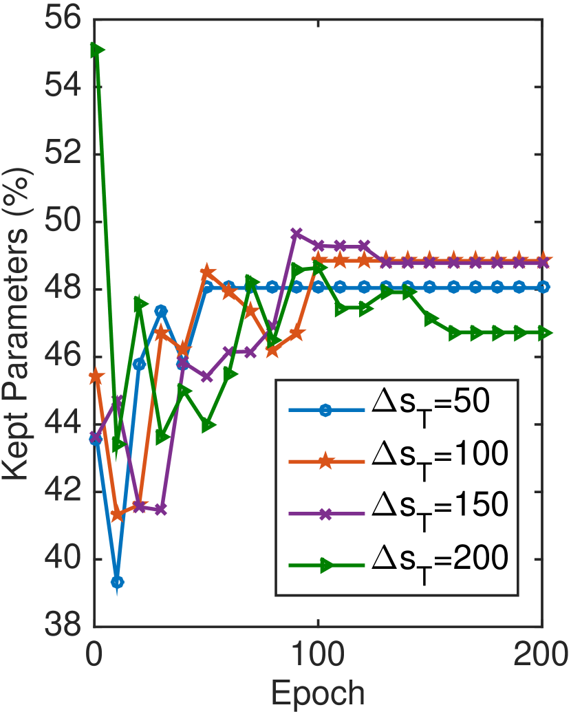
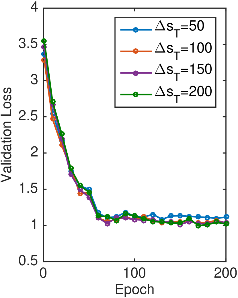
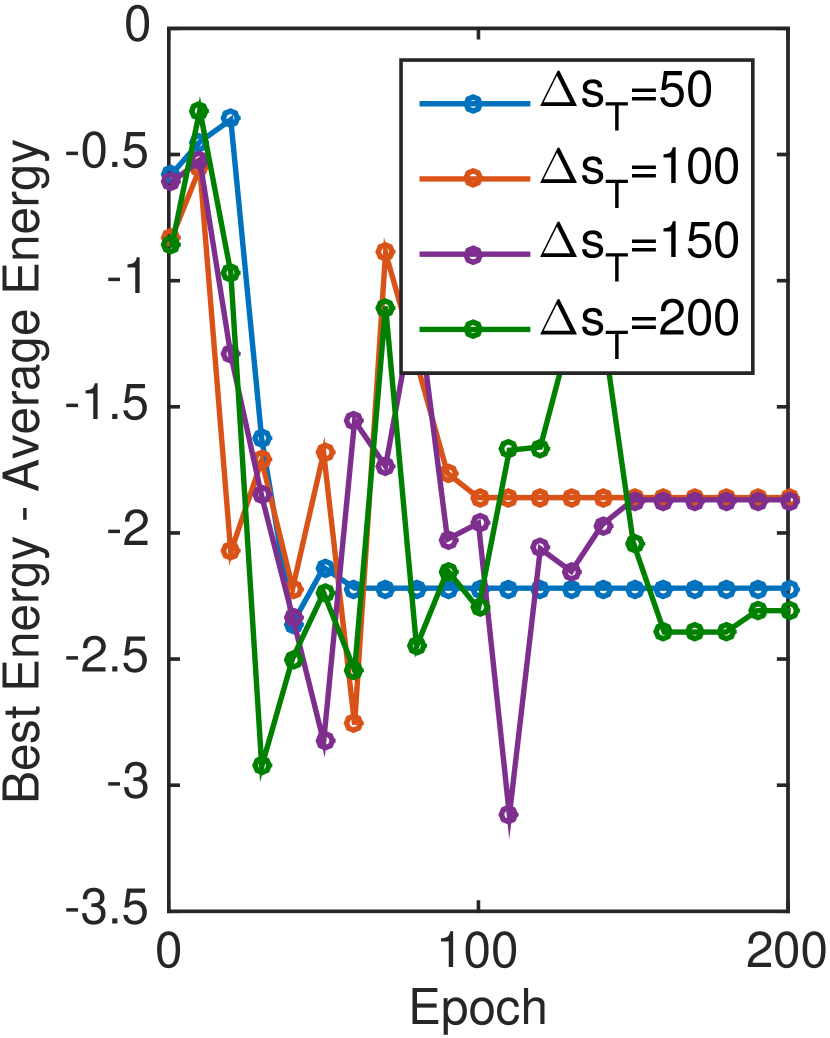
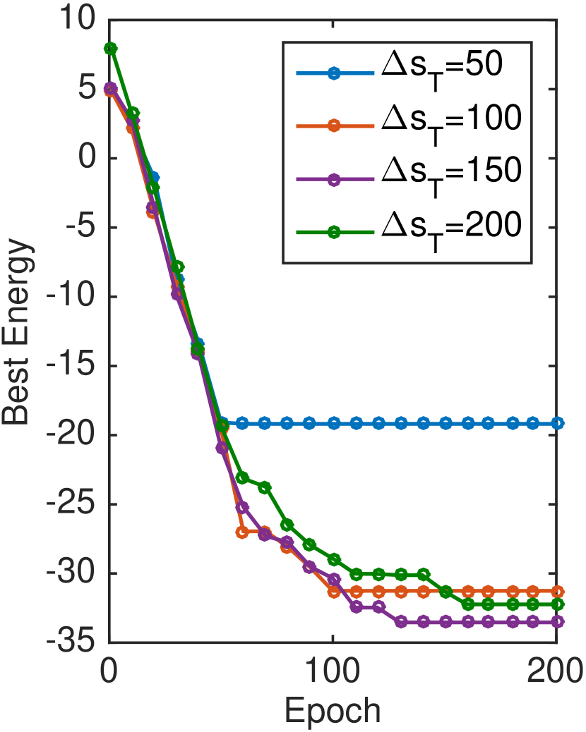
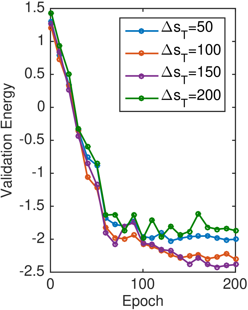
Balancing the exploration of optimizer for a feasible state vector while giving enough time for fine-tuning that state is crucial. However, EDropout combines the state selection and training in the first phase and ultimately can naturally converge to a best state vector based on the energy of the states or manually be controlled by $\Delta\mathbf{s}_{T}$. Figure 9(a) shows convergence of the kept number of parameters for $\Delta\mathbf{s}_{T}\in\{50,100,150,200\}$. For $\Delta\mathbf{s}_{T}=150$ and $\Delta\mathbf{s}_{T}=200$ the model has converged approximately at epochs 125 and 160, respectively. Figure 9(c) shows the value of $\Delta\mathbf{s}$ defined in (11), whereas $|\Delta\mathbf{s}|\rightarrow 0$ suggests the algorithm is moving toward exploitation (less diversity of candidate states) and as $|\Delta\mathbf{s}|\rightarrow\infty$ it is moving toward exploration of the optimization landscape (more diversity of candidate states). This shows importance of using $\Delta\mathbf{s}_{T}$ as an added early state convergence metric, since even-though setting $\Delta\mathbf{s}_{T}=200$ has achieved a smaller number of parameters at approximately epoch 160, it decreases the chance of fine-tuning in the remaining epochs, resulting in an increase in the validation energy as plotted in Figure 9(e). Since we are minimizing the energy loss, it is obvious that $\Delta\mathbf{s}\leq 0$ is guaranteed in (11). The interesting observation is the pre-mature convergence of $\Delta\mathbf{s}_{T}=50$ and over-fitting of $\Delta\mathbf{s}_{T}=200$ in terms of the best energy and validation energy in Figures 9(d) and 9(e). The results in Table III suggest $\Delta\mathbf{s}_{T}=100$ is a good threshold, since it has the highest Top-1 accuracy and also fairly splits half of the training budget for exploring and the other half for fine-tuning. This threshold is used for the rest of the experiments.

IV-D2 Number of Candidate State Vectors

A large number of candidate state vectors (i.e. the population size) $S$ increases the exploration of the optimization landscape and meanwhile the stagnation risk. On the other hand, a small population (${S\leq 8}$, [19]) size encourages exploitation and fine-tuning of optimization. Different methods have been proposed to control this parameter. It has been shown in [19] that it is possible to maintain a high exploration capability while using a small population size by using a vectorized-random mutation factor (VRMF) trick. To analyze $S$, we trained ResNet-18 using EDropout for $S\in\{8,16,32,64,128,256\}$ and the Flowers dataset. Table III shows that the small population size $S=8$ and diversified with VRMF achieves the best Top-1 score. However, larger $S$ results in more pruning rate at a lower loss value. Figure 11 shows the rate of kept parameter and the best energy of the model during training epochs on the validation dataset, where $\Delta\mathbf{s}_{T}=100$. The plots show that smaller $S$ converges faster to a lower energy while larger $S$ has slower progress and is more prone to stagnation. Since the results show very competitive performance between various values of $S$, we use $S=8$ for the rest of the experiments.

IV-D3 States Initialization

The probability $P$ in ${s_{i,d}^{(0)}\sim Bernoulli(P)}$ governs the number of dropped/pruned trainable parameters for each state vector $\mathbf{s}_{i}$ at the initialization stage. If a specific pruning rate is desired, it is possible to define constraints in the evolution phase. Figure 11 shows convergence of ResNet-18 with EDropout using $P\in\{0.2,0.4,0.6,0.8,1\}$ on the Flowers validation dataset and the corresponding classification results on the test dataset are in Table III. The results show that at the beginning of training there is diversity in the number of kept parameters but the plots converge to a number in the range of $[45\%,48\%]$. However, this affects the best energy, where the model with smaller $P$ converges to a lower energy. Since the results show a little sensitivity of the models to $P$ and convergence to approximately $50\%$ pruning rate, $P$ is set to $0.5$.

IV-E Classification Performance Analysis

An original model contains the entire possible trainable parameters and has a larger learning capacity than the corresponding pruned model. EDropout is discussed in pruned (P) and full (F) modes. The pruned mode refers to performing inference with the pruned network and the full mode refers to training the original model with EDropout and using the entire trainable parameters for inference. We use the pruning rate chosen by EDropout as the pruning rate for Deep Compression [1].

IV-E1 Kuzushiji Dataset

Kuzushiji dataset is a fairly easy dataset and performance results of ResNets are very close to each other as shown in Table IV(f)(a). For example, the Top-1 accuracy of ResNet-18 and ResNet-101 is $98.23\%$ and $98.26\%$, respectively, which means overparameterization of ResNets from $11.1$M to $42.5$M only $0.03\%$ increases the Top-1 accuracy. The Top-1 accuracy of ResNet-18+EDropout(P) and ResNet-101+EDropout(P) is $97.78\%$ and $98.05\%$, respectively, where the performance has increased $0.27\%$ and the pruning rate has also increased from $48.51\%$ to $54\%$, respectively. Top-1 accuracy of ResNet-50 is $97.70\%$ and ResNet-50+ThiNet, which has a pruning rate of $55.96\%$, achieves about $2\%$ lower accuracy. ResNet-50+ThiNet has a slightly larger loss value (i.e. $0.2278$) than the ResNet-50+DC (i.e. $0.2142$), but its Top-1 accuracy is $1.38\%$ higher. ResNet-50+EDropout(P) has the closest performance to the original model among the pruning models at a pruning rate of $54.43\%$ and a Top-1 accuracy of $97.63\%$, which is $0.07\%$ lower than ResNet-50.

ChannelNet-v2 has the best Top-1 performance in Table V(f)(a) with $1.8$M parameters. However, its pruning rate is $0\%$ since it is not a pruning method. AlexNet has $57$M parameters and a Top-1 accuracy of $97.77\%$. SqueezeNet is a compact version of AlexNet and has achieved $97.19\%$ Top-1 accuracy with $0.72$M number of parameters. EDropout has achieved a pruning rate of $21.43\%$ for AlexNet, which is inferior to the rate it has achieved in pruning ResNets. AlexNet+EDropout(P) has a Top-1 accuracy of $96.57\%$ which is $1.2\%$ lower than accuracy of AlexNet. EDropout can also be applied to SqueezeNet, where SqueezeNet+EDropout(P) has a Top-1 accuracy of $96.35\%$, which is $0.84\%$ lower than the performance of SqueezeNet.

a Kept parameters

b Validation loss

c Energy loss difference

d Best energy loss

Figure 12: Analysis of EDropout with ResNet-50 on the validation dataset of Kuzushiji, Fashion, CIFAR-10, CIFAR-100, Flowers, and ImageNet datasets with $S=8$, initialization probability of $P=0.5$, and $\Delta\mathbf{s}_{T}=100$.

IV-E2 Fashion Dataset

This dataset is more challenging than the Kuzushiji dataset. ResNet-18 has a Top-1 classification performance of $93.87\%$ on the Fashion dataset which is about $5\%$ lower than the Kuzushiji dataset, Table IV(f)(b). ResNet-50+ThiNet has a higher Top-1 accuracy than Deep Compression in pruning ResNet-50 with a smaller number of parameters (i.e. $10.3$M). EDropout can prune ResNet-50 at a rate of $54.86\%$ with a Top-1 accuracy of $92.97\%$, which has the best pruning performance for ResNet-50.

Table V(f)(b) shows that ChannelNet-v2 with $1.7$M number of parameters has a Top-1 accuracy of $93.41\%$. However, SqueezeNet with $0.72$M parameters has a Top-1 accuracy of $92.64\%$ which is only $0.77\%$ lower than ChannelNet-v2. EDropout can further reduce the number of parameters in SqueezeNet to $0.38$M while keeping the performance very close (about $0.3\%$ lower) to the original SqueezeNet.

IV-E3 CIFAR-10 Dataset

Table IV(f)(c) shows that ResNet-50+ThiNet has a Top-1 accuracy of $79.83\%$ with a pruning rate of $56.18\%$ and ResNet-50 has a Top-1 accuracy of $92.21\%$ with $23.5$M parameters. ResNet-50+DC has approximately $25\%$ lower Top-1 accuracy than the original model. ResNet-50+EDropout(P) has the best performance with a Top-1 accuracy of $85.30\%$ and $10.9$M parameters.

Table V(f)(c) shows that AlexNet has a Top-1 accuracy of $84.32\%$ with $57.4$M parameters. EDropout applied on the AlexNet model could prune $22.64\%$ of the parameters but the accuracy drops to $74.66\%$. SqueezeNet, which has $0.73$M parameters, has an accuracy of $81.49\%$ where EDropout can prune $47.65\%$ of its parameters with $4.64\%$ drop of Top-1 performance. The results show that EDropout has better performance than the other methods in pruning original models with a slight drop of performance. Particularly, with respect to the Top-3 and Top-5 metrics.

IV-E4 CIFAR-100 Dataset

CIFAR-100 has $100$ data classes which increases its classification complexity. ResNet-101 with $42.6$M parameters can achieve $71.19\%$ Top-1 accuracy as shown in Table IV(f)(d). Similar to the previous experiments, EDropout has a better performance than the other methods with a Top-1 classification performance of $61.92\%$ and $18.6$M number of parameters, which has about $9.27\%$ lower Top-1 performance than the ResNet-101 at full capacity.

Table V(f)(d) shows that AlexNet+EDropout(P) has a Top-1 performance of $56.59\%$ with $41.2$M parameters, which has $3.53\%$ lower Top-1 accuracy than AlexNet with $57.4$M parameters. EDropout can also decrease the number of parameters in SqueezeNet from $0.77$M to $0.43$M with $3.83\%$ drop of Top-1 accuracy.

IV-E5 Flowers Dataset

The Flowers dataset has $102$ number of classes and it is highly limited and imbalanced. Table IV(f)(e) shows that ResNet-101+EDropout(F) has the best Top-1 accuracy for ResNet-101 with $3.26\%$ drop of performance. The pruned version of EDropout has an accuracy of $58.17\%$ with $19.2$M number of parameters, which is $44.85\%$ of the ResNet-101 parameters.

Table V(f)(e) shows that AlexNet has $11\%$ higher Top-1 accuracy than SqueezeNet on the Flowers dataset, where AlexNet has $57.4$M parameters and SqueezeNet has $0.77$M parameters. SqueezeNet+EDropout(P) reduces the number of parameters in SqueezeNet to $0.57$M with almost $2.22\%$ of drop in Top-1 accuracy.

IV-E6 ImageNet Dataset

Table IV(f)(f) shows that EDropout has a relatively higher Top-1 accuracy than the other pruning models with respect to the pruning rate. ResNet-50+ThiNet has an accuracy of $72.11\%$ with $12.4$M parameters and ResNet-50+DC has an accuracy of $67.02\%$ with $10.2$M parameters, which are $3.16\%$ and $8.25\%$ lower than the Top-1 performance of ResNet-50, respectively. This is while ResNet-50+EDropout(P) has $1.55\%$ lower performance than ResNet-50 with $10.2$M parameters.

ChannelNet-v2 in Table V(f)(f) has a Top-1 accuracy of $69.5\%$ with $2.7$M parameters. SqueezeNet has an accuracy of $57.31\%$ with $1.3$M parameters and SqueezeNet+EDropout(P) achieves $0.7\%$ lower accuracy by pruning $39.68\%$ of the parameters. AlexNet has a Top-1 accuracy of $58.26\%$ with $60$M parameters and AlexNet+EDropout(P) decreases the number of parameters in AlexNet to $49.2$M at the cost of $2.23\%$ lower Top-1 performance.

IV-F Convergence Analysis

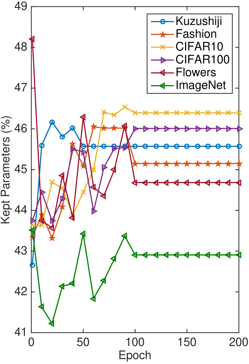
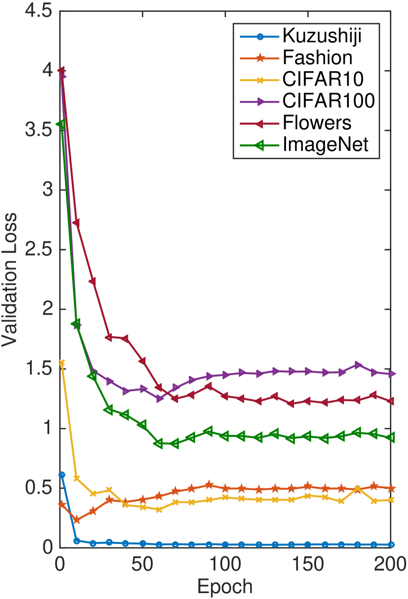
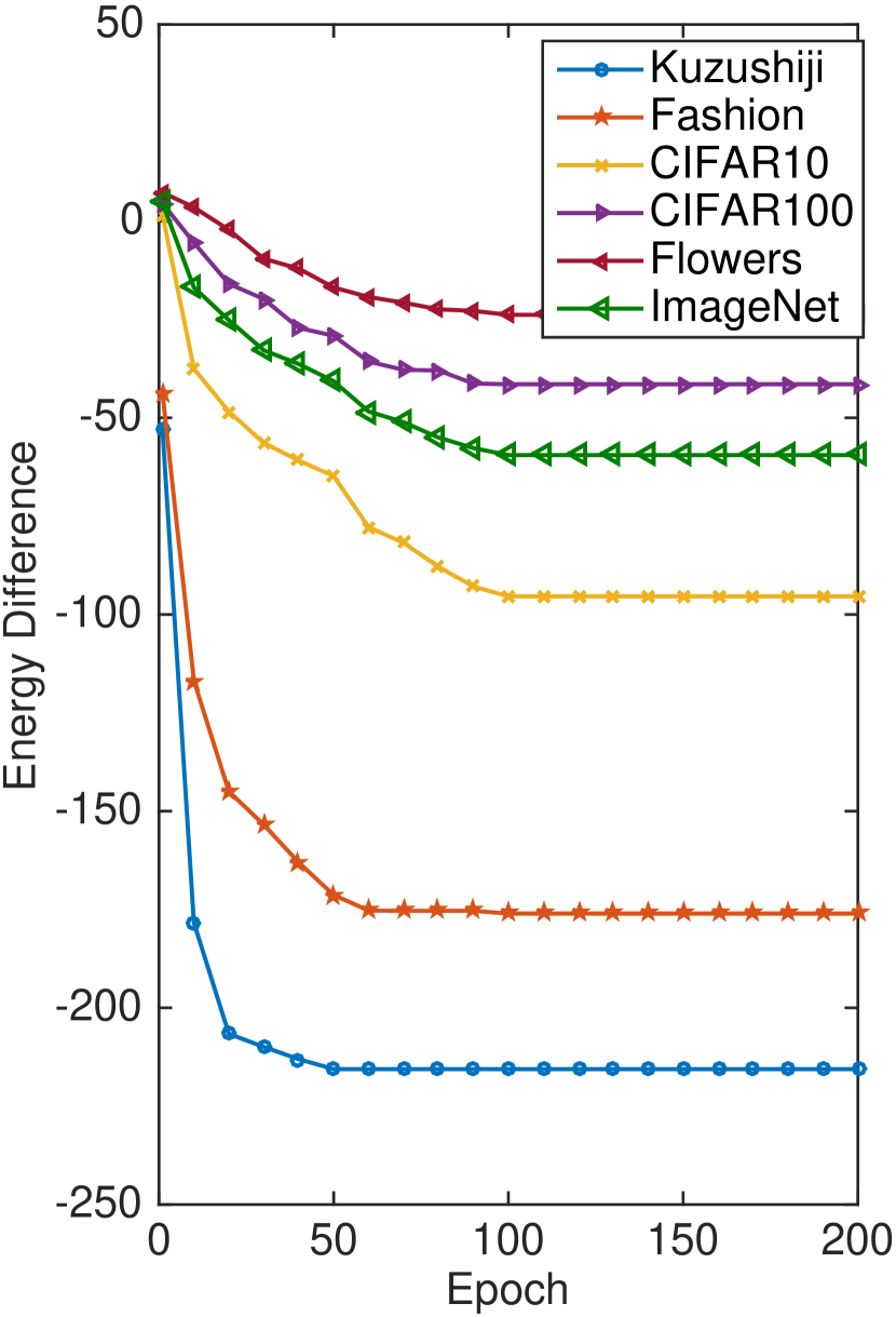
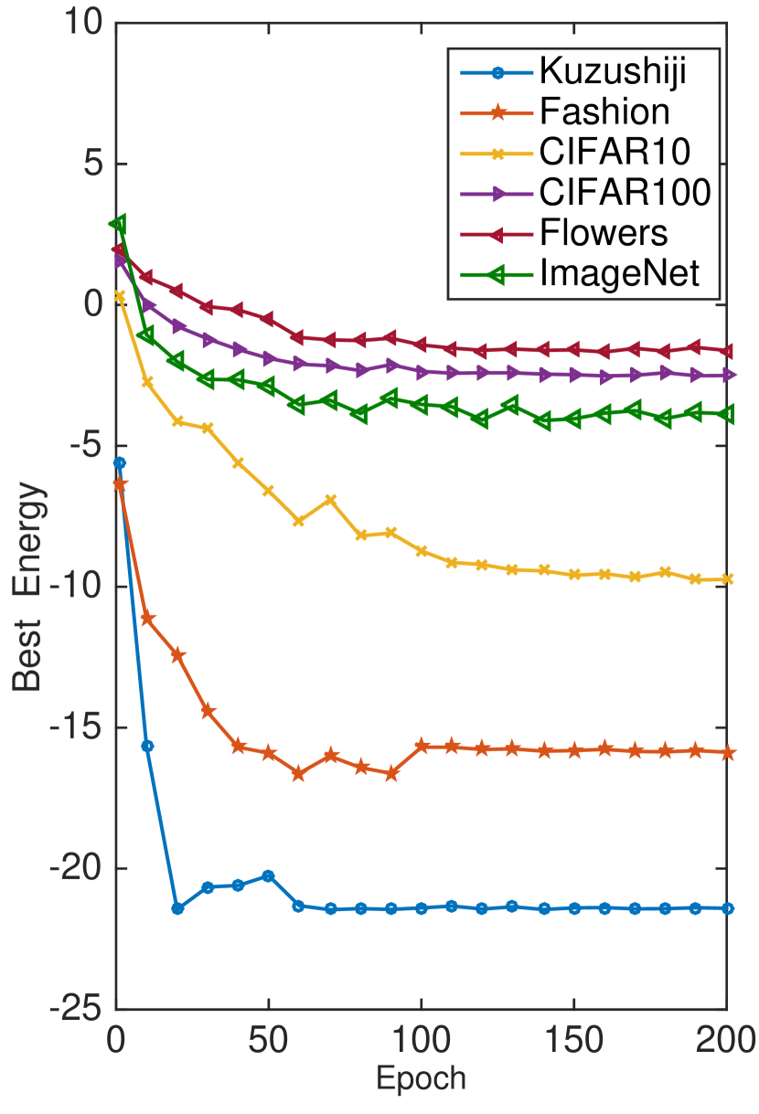
Figure 12 shows convergence plots of the validation datasets for ResNet-50 with EDropout. Figure 12(a) shows that after epoch $100$ the early state convergence is applied. EDropout+ResNet-50 converges to a range approximately between $43\%$ and $47\%$ of the total number of parameters in the original model. The CIFAR-100, Flowers, and ImageNet datasets have higher validation loss than the other datasets in Figure 12(b). EDropout+ResNet-50 converges faster for simple datasets such as Fashion comparing with the more challenging ones. The other observation is that complex datasets, in terms of number of classes, number of training samples, number of image channels, and input image size, have higher best energy values, which reflects more number of parameters are required to train a model to perform classification in these datasets. As an example, the Flowers dataset in Figure 12(d) has the highest best energy values while the Kuzushiji dataset has the lowest energy values. Similar trend is observable in the energy loss difference (i.e. difference between the best energy of the population and the average energy of the population) plots in Figure 12(c).

TABLE VI: Training time (in seconds/iteration) for the population size $S\in\{8,32\}$ and a batch size of 128 using CIFAR-10.
HTML]9AFF99  E-3 HTML]32CB00  E-2 HTML]009901  E-1

Model Original EDropout S=8 EDropout S=32 EDropout Parallel S=8 EDropout Parallel S=32 AlexNet [HTML]9AFF994.14E-3 [HTML]32CB001.26E-2 [HTML]32CB005.06E-2 [HTML]9AFF998.01E-3 [HTML]32CB002.67E-2 ResNet-18 [HTML]9AFF997.11E-3 [HTML]32CB002.93E-2 [HTML]0099011.19E-1 [HTML]32CB002.15E-2 [HTML]32CB006.33E-2 ResNet-34 [HTML]32CB001.13E-2 [HTML]32CB005.03E-2 [HTML]0099011.87E-1 [HTML]32CB003.62E-2 [HTML]32CB008.28E-2 ResNet-50 [HTML]32CB001.63E-2 [HTML]32CB007.46E-2 [HTML]0099012.90E-1 [HTML]32CB005.45E-2 [HTML]0099011.42E-1 ResNet-101 [HTML]32CB005.20E-2 [HTML]0099011.62E-1 [HTML]0099015.46E-1 [HTML]0099011.14E-1 [HTML]0099012.74E-1

IV-G Computational Complexity Analysis

The main drawback of EDropout is its computational complexity as a result of using a population of state vectors in the optimization phase to prune a network.

The major operations in training a neural network are feedforward (inference) and backpropagation. In order to provide a theoretical framework, let us define the feedforward time per iteration as $T_{inf}$ and the backpropagation time per iteration as $T_{bp}$. We also assume ${T_{inf}(EDropout)\approx T_{inf}(Net)}$ and ${T_{bp}(EDropout)\approx T_{bp}(Net)}$ for simplicity, where $Net$ refers to the original network. Hence, we can define the total training time of an original network as

$$T(Net)=N_{epoch}N_{batch}(T_{inf}+T_{bp}).$$ (12)

EDropout has another major operation which is the evolution of the population of candidate state vectors. Hence, the training time of EDropout applied on an original network is

$$T(EDropout)=N_{epoch}N_{batch}(S\cdot T_{inf}+T_{bp}+T_{evn}),$$ (13)

where $T_{evn}$ is the evolution time per training iteration.

a Upper boundary of number of inference calls for different population sizes $S$ and different number of training samples (the datasets in one line of legend have similar number of training samples). The Inference Calls axis is log scaled.

b Inference time of ResNet-18 for different data batch sizes in seconds/image. The Time axis is log scaled.

Figure 13: Computational complexity of EDropout with respect to the number of inference calls and inference time per image.

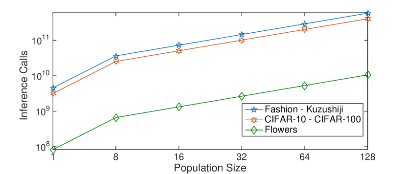
In the worst-case scenario (i.e. without considering the early state convergence), for $N_{epoch}$ number of epochs and $N_{batch}$ number of iterations per epoch, the upper bound for the number of inference calls (i.e. performing inference) is $S\cdot N_{epoch}\cdot N_{batch}$, that is $S$ times more than one inference per training iteration, as demonstrated in Figure 13(a) for 200 training epochs. By considering the early state convergence condition met after $\Delta s_{T}$ training epochs, $T(EDropout)$ becomes

$$\begin{split}T(EDropout;\Delta s_{T})&=\underbrace{\Delta s_{T}\cdot N_{batch}(S\cdot T_{inf}+T_{bp}+T_{evn})}_{\text{exploration}}\\ &+\underbrace{(N_{epoch}-\Delta s_{T})\cdot N_{batch}\cdot(T_{inf}+T_{bp})}_{\text{fine-tuning}}\\ &=\underbrace{N_{epoch}N_{batch}(T_{inf}+T_{bp})}_{\textit{T(Net)}}\\ &+\underbrace{N_{batch}\Delta s_{T}\big{(}T_{evn}+(S-1)T_{inf}\big{)}}_{\text{EDropout overhead}},\end{split}$$ (14)

where $\Delta s_{T}\leq N_{epoch}$.

Table VI shows the comparison between $T(EDropout)$ and $T(Net)$ per training iteration for a batch size of 128 using the CIFAR-10 dataset. The benefit of the computational overhead of EDropout is the added diversity in searching for the sub-network with lower energy. Since the candidate states in the population are independent, one can implement the optimizer in parallel at the state vector level, which shows dramatic reduction of the $T(EDropout)$ in Table VI.

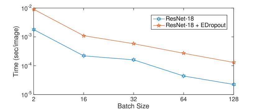
It is obvious that increasing the data batch size for each iteration can also decrease the training time. As an example, Figure 13(b) shows that increasing the batch size can decrease the training and inference time of ResNet-18. Another approach which reduces the execution time is using the concept of early state convergence, where the number of iterations for sub-network exploration can be defined or adaptively set by the model according to (11), as discussed in Subsection III-C4.

V Conclusions

In this paper, we introduce the concept of energy-based dropout and pruning in deep neural networks. We propose a new method for partial training of deep neural networks (DNNs) based on the concept of dropout. An energy model is proposed to compute energy loss of a population of binary candidate pruning state vectors, where each vector represents a sub-network of the DNN. An evolutionary technique searches the population of state vectors, selects the state vector with lowest energy loss in that iteration, and trains the corresponding sub-network using backpropagation. Ultimately, the states can converge to a best state and the algorithm continues fine-tuning the corresponding sub-network, which is equivalent to pruning of the DNN. The results show that there is a trade-off between network size and classification accuracy. The proposed method can reduce (approximately $50\%$ on average) the number of parameters in the inference network while keeping the classification accuracy competitive to the original network.

VI Acknowledgment

The authors acknowledge financial support and access to the Digital Annealer (DA) of Fujitsu Laboratories Ltd. and Fujitsu Consulting (Canada) Inc.

Hojjat Salehinejad is a PhD candidate at the Edward S. Rogers Sr. Department of Electrical and Computer Engineering, University of Toronto. His research focus is on machine learning and signal processing. He is a member of IEEE Signal Processing Society and has served as a reviewer for various IEEE conferences and journals.

Shahrokh Valaee is a Professor with the Edward S. Rogers Sr. Department of Electrical and Computer Engineering, University of Toronto, and the holder of Nortel Chair of Network Architectures and Services. He is the Founder and the Director of the Wireless and Internet Research Laboratory (WIRLab) at the University of Toronto. Professor Valaee was the TPC Co-Chair and the Local Organization Chair of the IEEE Personal Mobile Indoor Radio Communication (PIMRC) Symposium 2011. He was the TCP Chair of PIMRC2017, the Track Co-Chair of WCNC 2014, the TPC Co-Chair of ICT 2015. He has been the guest editor for various journals. He was a Track Co-chair for PIMRC 2020 and VTC Fall 2020. From December 2010 to December 2012, he was the Associate Editor of the IEEE Signal Processing Letters. From 2010 to 2015, he served as an Editor of IEEE Transactions on Wireless Communications. Currently, he is an Editor of Journal of Computer and System Science. Professor Valaee is a Fellow of the Engineering Institute of Canada, and a Fellow of IEEE.

References

- [1] S. Han, H. Mao, and W. J. Dally, “Deep compression: Compressing deep neural networks with pruning, trained quantization and huffman coding,” arXiv preprint arXiv:1510.00149, 2015.
- [2] N. Srivastava, G. Hinton, A. Krizhevsky, I. Sutskever, and R. Salakhutdinov, “Dropout: a simple way to prevent neural networks from overfitting,” The Journal of Machine Learning Research, vol. 15, no. 1, pp. 1929–1958, 2014.
- [3] T. Hastie, R. Tibshirani, and M. Wainwright, Statistical learning with sparsity: the lasso and generalizations. CRC press, 2015.
- [4] J. Ba and B. Frey, “Adaptive dropout for training deep neural networks,” in Advances in Neural Information Processing Systems, 2013, pp. 3084–3092.
- [5] D. P. Kingma, T. Salimans, and M. Welling, “Variational dropout and the local reparameterization trick,” in Advances in Neural Information Processing Systems, 2015, pp. 2575–2583.
- [6] S. Park, J. Park, S.-J. Shin, and I.-C. Moon, “Adversarial dropout for supervised and semi-supervised learning,” in Thirty-Second AAAI Conference on Artificial Intelligence, 2018.
- [7] L. Wan, M. Zeiler, S. Zhang, Y. Le Cun, and R. Fergus, “Regularization of neural networks using dropconnect,” in International conference on machine learning, 2013, pp. 1058–1066.
- [8] A. Labach, H. Salehinejad, and S. Valaee, “Survey of dropout methods for deep neural networks,” arXiv preprint arXiv:1904.13310, 2019.
- [9] Y. LeCun, J. S. Denker, and S. A. Solla, “Optimal brain damage,” in Advances in neural information processing systems, 1990, pp. 598–605.
- [10] Z. Liu, M. Sun, T. Zhou, G. Huang, and T. Darrell, “Rethinking the value of network pruning,” arXiv preprint arXiv:1810.05270, 2018.
- [11] S. J. Nowlan and G. E. Hinton, “Simplifying neural networks by soft weight-sharing,” Neural computation, vol. 4, no. 4, pp. 473–493, 1992.
- [12] K. Ullrich, E. Meeds, and M. Welling, “Soft weight-sharing for neural network compression,” arXiv preprint arXiv:1702.04008, 2017.
- [13] H. Salehinejad and S. Valaee, “Ising-dropout: A regularization method for training and compression of deep neural networks,” in ICASSP 2019-2019 IEEE International Conference on Acoustics, Speech and Signal Processing (ICASSP). IEEE, 2019, pp. 3602–3606.
- [14] S. Matsubara, H. Tamura, M. Takatsu, D. Yoo, B. Vatankhahghadim, H. Yamasaki, T. Miyazawa, S. Tsukamoto, Y. Watanabe, K. Takemoto et al., “Ising-model optimizer with parallel-trial bit-sieve engine,” in Conference on Complex, Intelligent, and Software Intensive Systems. Springer, 2017, pp. 432–438.
- [15] H. Salehinejad, Z. Wang, and S. Valaee, “Ising dropout with node grouping for training and compression of deep neural networks,” in 2019 IEEE Global Conference on Signal and Information Processing (GlobalSIP). IEEE, 2019, pp. 1–5.
- [16] H. Salehinejad and S. Valaee, “Pruning of convolutional neural networks using ising energy model,” arXiv preprint arXiv:2102.05437, 2021.
- [17] Y. LeCun, S. Chopra, R. Hadsell, M. Ranzato, and F. Huang, “A tutorial on energy-based learning,” Predicting structured data, vol. 1, no. 0, 2006.
- [18] K. V. Price, “Differential evolution,” pp. 187–214, 2013.
- [19] H. Salehinejad, S. Rahnamayan, and H. R. Tizhoosh, “Micro-differential evolution: Diversity enhancement and a comparative study,” Applied Soft Computing, vol. 52, pp. 812–833, 2017.
- [20] S. Anwar, K. Hwang, and W. Sung, “Structured pruning of deep convolutional neural networks,” ACM Journal on Emerging Technologies in Computing Systems (JETC), vol. 13, no. 3, pp. 1–18, 2017.
- [21] W. Grathwohl, K.-C. Wang, J.-H. Jacobsen, D. Duvenaud, M. Norouzi, and K. Swersky, “Your classifier is secretly an energy based model and you should treat it like one,” arXiv preprint arXiv:1912.03263, 2019.
- [22] A. Labach and S. Valaee, “A framework for neural network pruning using gibbs distributions,” arXiv preprint arXiv:2006.04981, 2020.
- [23] G. Hinton, O. Vinyals, and J. Dean, “Distilling the knowledge in a neural network,” arXiv preprint arXiv:1503.02531, 2015.
- [24] D. Barber and A. Botev, “Dealing with a large number of classes–likelihood, discrimination or ranking?” arXiv preprint arXiv:1606.06959, 2016.
- [25] R. M. Neal, “Annealed importance sampling,” Statistics and computing, vol. 11, no. 2, pp. 125–139, 2001.
- [26] T. Mikolov, I. Sutskever, K. Chen, G. Corrado, and J. Dean, “Distributed representations of words and phrases and their compositionality,” arXiv preprint arXiv:1310.4546, 2013.
- [27] H. Salehinejad, R. Zadeh, R. Liscano, and S. Rahnamayan, “3d localization in large-scale wireless sensor networks: A micro-differential evolution approach,” in 2014 IEEE 25th Annual International Symposium on Personal, Indoor, and Mobile Radio Communication (PIMRC). IEEE, 2014, pp. 1824–1828.
- [28] H. Salehinejad, S. Rahnamayan, and H. R. Tizhoosh, “Type-ii opposition-based differential evolution,” in 2014 IEEE Congress on Evolutionary Computation (CEC). IEEE, 2014, pp. 1768–1775.
- [29] K. P. Murphy, Machine learning: a probabilistic perspective. MIT press, 2012.
- [30] J. Lampinen, I. Zelinka et al., “On stagnation of the differential evolution algorithm,” in Proceedings of MENDEL, 2000, pp. 76–83.
- [31] H. Xiao, K. Rasul, and R. Vollgraf. (2017) Fashion-mnist: a novel image dataset for benchmarking machine learning algorithms.
- [32] T. Clanuwat, M. Bober-Irizar, A. Kitamoto, A. Lamb, K. Yamamoto, and D. Ha. (2018) Deep learning for classical japanese literature.
- [33] A. Krizhevsky, G. Hinton et al., “Learning multiple layers of features from tiny images,” 2009.
- [34] M.-E. Nilsback and A. Zisserman, “Automated flower classification over a large number of classes,” in 2008 Sixth Indian Conference on Computer Vision, Graphics & Image Processing. IEEE, 2008, pp. 722–729.
- [35] J. Deng, W. Dong, R. Socher, L.-J. Li, K. Li, and L. Fei-Fei, “Imagenet: A large-scale hierarchical image database,” in 2009 IEEE conference on computer vision and pattern recognition. Ieee, 2009, pp. 248–255.
- [36] T. DeVries and G. W. Taylor, “Improved regularization of convolutional neural networks with cutout,” arXiv preprint arXiv:1708.04552, 2017.
- [37] A. Krizhevsky, I. Sutskever, and G. E. Hinton, “Imagenet classification with deep convolutional neural networks,” in Advances in neural information processing systems, 2012, pp. 1097–1105.
- [38] F. N. Iandola, S. Han, M. W. Moskewicz, K. Ashraf, W. J. Dally, and K. Keutzer, “Squeezenet: Alexnet-level accuracy with 50x fewer parameters and¡ 0.5 mb model size,” arXiv preprint arXiv:1602.07360, 2016.
- [39] K. He, X. Zhang, S. Ren, and J. Sun, “Deep residual learning for image recognition,” in Proceedings of the IEEE conference on computer vision and pattern recognition, 2016, pp. 770–778.
- [40] H. Li, A. Kadav, I. Durdanovic, H. Samet, and H. P. Graf, “Pruning filters for efficient convnets,” arXiv preprint arXiv:1608.08710, 2016.
- [41] J.-H. Luo, J. Wu, and W. Lin, “Thinet: A filter level pruning method for deep neural network compression,” in Proceedings of the IEEE international conference on computer vision, 2017, pp. 5058–5066.
- [42] H. Gao, Z. Wang, and S. Ji, “Channelnets: Compact and efficient convolutional neural networks via channel-wise convolutions,” in Advances in neural information processing systems, 2018, pp. 5197–5205.
- [43] A. G. Howard, M. Zhu, B. Chen, D. Kalenichenko, W. Wang, T. Weyand, M. Andreetto, and H. Adam, “Mobilenets: Efficient convolutional neural networks for mobile vision applications,” arXiv preprint arXiv:1704.04861, 2017.
- [44] M. D. Zeiler, “Adadelta: an adaptive learning rate method,” arXiv preprint arXiv:1212.5701, 2012.
- [45] N. Takahashi, M. Gygli, and L. Van Gool, “Aenet: Learning deep audio features for video analysis,” arXiv preprint arXiv:1701.00599, 2017.
![[Uncaptioned image]](/html/2006.04270/assets/x30.png) |