CERN-TH-2020-084, LAPTH-027/20, MPP-2020-75

MINNLO${}_{\text{PS}}$: Optimizing $2\rightarrow 1$ hadronic processes

Abstract

We consider the MiNNLO_PS method to consistently combine next-to-next-to-leading order (NNLO) QCD calculations with parton-shower simulations. We identify the main sources of differences between MiNNLO_PS and fixed-order NNLO predictions for inclusive observables due to corrections beyond NNLO accuracy and present simple prescriptions to either reduce or remove them. Refined predictions are presented for Higgs, charged- and neutral-current Drell Yan production. The agreement with fixed-order NNLO calculations is considerably improved for inclusive observables and scale uncertainties are reduced. The codes are released within the POWHEG-BOX.

1 Introduction

Precision studies play a crucial role in the rich physics programme at the Large Hadron Collider (LHC). Not only do they enable the accurate determination of Standard-Model (SM) rates and parameters, but they also provide a valuable route to the discovery of new-physics phenomena through small deviations from the SM. Experimental analyses rely on parton-shower simulations to generate fully exclusive events. Therefore, in order to fully exploit the vast amount high-quality data collected at the LHC, it is now paramount to include highest-order perturbative information in event simulation.

The consistent combination of next-to-next-to-leading order (NNLO) QCD calculations with parton-shower simulations (NNLO+PS) is one of the current challenges in collider theory, and it is indispensable to provide the interface between accurate theory predictions and precision measurements. Four NNLO+PS methods [1, 2, 3, 4], which rely on different theoretical formulations, have been proposed in the past decade. A good NNLO+PS method should attain NNLO accuracy for observables inclusive in the QCD radiation beyond the Born level, while preserving the logarithmic structure (and accuracy) of the parton-shower simulation after matching. While NNLO accuracy is guaranteed by all existing methods, the kinematic constraints that each of the above methods impose on the subsequent parton-shower evolution may have consequences in terms of the logarithmic accuracy of the final simulation. In Ref. [4] we have presented the method MiNNLO_PS, which has the following features:

• NNLO corrections are calculated directly during the generation of the events and without additional reweighting.

• No merging scale is required to separate different multiplicities in the generated event samples.

• The matching to the parton shower is performed according to the POWHEG method [5] and preserves the leading logarithmic (LL) structure for transverse-momentum ordered showers.

In this article we investigate the sources of differences between MiNNLO_PS and fixed-order NNLO (f NNLO) QCD predictions due to higher-order corrections beyond the nominal perturbative accuracy. These differences affect inclusive observables such as the total cross section or the rapidity distribution of a color-singlet produced in hadronic collisions. We identify the main sources of such corrections, which stem from:

1. Presence of higher-order terms (i.e. beyond NNLO) in the matching formula;

2. Scale setting in the QCD running coupling and in the parton distribution functions (PDFs);

3. Higher-order effects due to the parton shower recoil scheme.

We introduce various prescriptions to either remove or reduce these corrections. This leads to a significantly improved agreement between MiNNLO_PS predictions and f NNLO calculations for inclusive observables. As a case study we focus on $2\rightarrow 1$ processes at the LHC, including Higgs boson production as well as charged-current and neutral-current Drell Yan (DY) production, and we present updated predictions that supersede those given in Ref. [4]. The computer codes with the implementation of the MiNNLO_PS method for $2\rightarrow 1$ processes is released with this article within the POWHEG-BOX framework [5, 7, 8].

2 MINNLO${}_{\text{PS}}$ in a nutshell

The MiNNLO_PS method [4] formulates a NNLO calculation fully differential in the phase space $\Phi_{\scriptscriptstyle\rm F}$ of the produced colour singlet ${\rm F}$ with invariant mass $Q$. It starts from a differential description of the production of the colour singlet and a jet (${\rm FJ}$), whose phase space we denote by $\Phi_{\scriptscriptstyle\rm FJ}$:

$$\frac{\mathrm{d}\sigma}{\mathrm{d}\Phi_{\scriptscriptstyle\rm FJ}}={\bar{B}}(\Phi_{\scriptscriptstyle\rm FJ})\times\bigg{\{}\Delta_{\rm pwg}(\Lambda_{\rm pwg})+\int\mathrm{d}\Phi_{\operatorname{rad}}\Delta_{\rm pwg}({p_{\text{T,rad}}})\frac{R(\Phi_{\scriptscriptstyle\rm FJ}{},\Phi_{\operatorname{rad}})}{B(\Phi_{\scriptscriptstyle\rm FJ}{})}\bigg{\}}\,,$$ (1)

where ${\bar{B}}(\Phi_{\scriptscriptstyle\rm FJ})$ generates the first radiation, while the content of the curly brackets describes the generation of the second radiation according to the POWHEG method [5, 7, 8]. Here, $B$ and $R$ are the squared tree-level matrix elements for ${\rm FJ}$ and ${\rm FJJ}$ production, respectively. $\Delta_{\rm pwg}$ denotes the POWHEG Sudakov form factor [5] and $\Phi_{\operatorname{rad}}$ (${p_{\text{T,rad}}}$) is the phase space (transverse momentum) of the second radiation. The POWHEG cutoff $\Lambda_{\rm pwg}$ is used in the generation of the second radiation and its default value is $\Lambda_{\rm pwg}=0.89$ GeV. The parton shower then adds additional radiation to Eq. (1) that contributes beyond $\mathcal{O}(\alpha_{\mathrm{S}}^{2}(Q))$ at all orders in perturbation theory. We refer to the explicit formulae of the original publications [5, 7, 8].

The function ${\bar{B}}(\Phi_{\scriptscriptstyle\rm FJ})$ is the central ingredient of MiNNLO_PS. Its derivation [4] stems from the observation that the NNLO cross section differential in the transverse momentum of the color singlet (${p_{\text{T}}}$) and in the Born phase space $\Phi_{\scriptscriptstyle\rm F}$ is described by the following formula

$$\frac{\mathrm{d}\sigma}{\mathrm{d}\Phi_{\scriptscriptstyle\rm F}\mathrm{d}{p_{\text{T}}}} =\frac{\mathrm{d}}{\mathrm{d}{p_{\text{T}}}}\bigg{\{}\exp[-\tilde{S}({p_{\text{T}}})]{\cal L}({p_{\text{T}}})\Bigg{\}}+R_{f}({p_{\text{T}}})=\exp[-\tilde{S}({p_{\text{T}}})]\left\{D({p_{\text{T}}})+\frac{R_{f}({p_{\text{T}}})}{\exp[-\tilde{S}({p_{\text{T}}})]}\right\}\,,$$ (2)

where $R_{f}$ contains terms that are non-singular in the ${p_{\text{T}}}\rightarrow 0$ limit, and

$$D({p_{\text{T}}})\equiv-\frac{\mathrm{d}\tilde{S}({p_{\text{T}}})}{\mathrm{d}{p_{\text{T}}}}{\cal L}({p_{\text{T}}})+\frac{\mathrm{d}{\cal L}({p_{\text{T}}})}{\mathrm{d}{p_{\text{T}}}}\,.$$ (3)

$\tilde{S}({p_{\text{T}}})$, defined in Eq. (24), represents the Sudakov form factor, while ${\cal L}({p_{\text{T}}})$ contains the parton luminosities, the squared virtual matrix elements for the underlying ${\rm F}$ production process up to two loops as well as the NNLO collinear coefficient functions and is given in Eq. (23) in Appendix A (see Ref. [4] for further details). A crucial feature of the MiNNLO_PS method is that the renormalisation and factorisation scales are set to ${\mu_{\text{R}}}\sim{\mu_{\text{F}}}\sim{p_{\text{T}}}$.

We introduce the NLO differential cross section for ${\rm FJ}$ production

$$\frac{\mathrm{d}\sigma^{\rm(NLO)}_{\scriptscriptstyle\rm FJ}}{\mathrm{d}\Phi_{\scriptscriptstyle\rm F}\mathrm{d}{p_{\text{T}}}}=\frac{\alpha_{\mathrm{S}}({p_{\text{T}}})}{2\pi}\left[\frac{\mathrm{d}\sigma_{\scriptscriptstyle\rm FJ}}{\mathrm{d}\Phi_{\scriptscriptstyle\rm F}\mathrm{d}{p_{\text{T}}}}\right]^{(1)}+\left(\frac{\alpha_{\mathrm{S}}({p_{\text{T}}})}{2\pi}\right)^{2}\left[\frac{\mathrm{d}\sigma_{\scriptscriptstyle\rm FJ}}{\mathrm{d}\Phi_{\scriptscriptstyle\rm F}\mathrm{d}{p_{\text{T}}}}\right]^{(2)}\,,$$ (4)

where $[X]^{(i)}$ denotes the coefficient of the $i$-th term in the perturbative expansion of the quantity $X$, which allows us to rewrite Eq. (2) as

$$\frac{\mathrm{d}\sigma}{\mathrm{d}\Phi_{\scriptscriptstyle\rm F}\mathrm{d}{p_{\text{T}}}} =\exp[-\tilde{S}({p_{\text{T}}})]\bigg{\{}\frac{\alpha_{\mathrm{S}}({p_{\text{T}}})}{2\pi}\left[\frac{\mathrm{d}\sigma_{\scriptscriptstyle\rm FJ}}{\mathrm{d}\Phi_{\scriptscriptstyle\rm F}\mathrm{d}{p_{\text{T}}}}\right]^{(1)}\left(1+\frac{\alpha_{\mathrm{S}}({p_{\text{T}}})}{2\pi}[\tilde{S}({p_{\text{T}}})]^{(1)}\right)+\left(\frac{\alpha_{\mathrm{S}}({p_{\text{T}}})}{2\pi}\right)^{2}\left[\frac{\mathrm{d}\sigma_{\scriptscriptstyle\rm FJ}}{\mathrm{d}\Phi_{\scriptscriptstyle\rm F}\mathrm{d}{p_{\text{T}}}}\right]^{(2)}$$

$$+\left[D({p_{\text{T}}})-\frac{\alpha_{\mathrm{S}}({p_{\text{T}}})}{2\pi}[D({p_{\text{T}}})]^{(1)}-\left(\frac{\alpha_{\mathrm{S}}({p_{\text{T}}})}{2\pi}\right)^{2}[D({p_{\text{T}}})]^{(2)}\right]+{\rm regular~{}terms~{}of~{}{\cal O}(\alpha_{\mathrm{S}}^{3})}\bigg{\}},$$ (5)

where the expressions of the $[D({p_{\text{T}}})]^{(i)}$ coefficients are given in Appendix A. The NNLO fully differential cross section is then obtained upon integration over ${p_{\text{T}}}$ from scales of the order of the Landau pole $\Lambda$ to the kinematic upper bound (we will discuss how to deal with the Landau divergence and integrate down to arbitrarily small ${p_{\text{T}}}$ in Section 3.2). Each term of Eq. (2) contributes to the total cross section with scales ${\mu_{\text{R}}}\sim{\mu_{\text{F}}}\sim Q$ according to the power counting formula

$$\int_{\Lambda}^{Q}\mathrm{d}{p_{\text{T}}}\frac{1}{{p_{\text{T}}}}\alpha_{\mathrm{S}}^{m}({p_{\text{T}}})\ln^{n}\frac{Q}{{p_{\text{T}}}}\exp(-\tilde{S}({p_{\text{T}}}))\approx{\cal O}\left(\alpha_{\mathrm{S}}^{m-\frac{n+1}{2}}(Q)\right)\,.$$ (6)

This suggests that one can expand the second line of Eq. (2), while neglecting terms that, upon integration over ${p_{\text{T}}}$, produce N³LO corrections or beyond to any inclusive observable in $\Phi_{\scriptscriptstyle\rm F}$. We can therefore truncate the second line of Eq. (2) to third order in $\alpha_{\mathrm{S}}({p_{\text{T}}})$

$$D({p_{\text{T}}})-\frac{\alpha_{\mathrm{S}}({p_{\text{T}}})}{2\pi}[D({p_{\text{T}}})]^{(1)}-\left(\frac{\alpha_{\mathrm{S}}({p_{\text{T}}})}{2\pi}\right)^{2}[D({p_{\text{T}}})]^{(2)}=\left(\frac{\alpha_{\mathrm{S}}({p_{\text{T}}})}{2\pi}\right)^{3}[D({p_{\text{T}}})]^{(3)}+{\cal O}(\alpha_{\mathrm{S}}^{4}({p_{\text{T}}}))\,.$$ (7)

The above considerations can be made at the fully differential level on the $\Phi_{\scriptscriptstyle\rm FJ}$ phase space, which leads to the definition of the ${\bar{B}}(\Phi_{\scriptscriptstyle\rm FJ})$ function as [4]

$${\bar{B}}(\Phi_{\scriptscriptstyle\rm FJ}) \equiv\exp[-\tilde{S}({p_{\text{T}}})]\bigg{\{}\frac{\alpha_{\mathrm{S}}({p_{\text{T}}})}{2\pi}\left[\frac{\mathrm{d}\sigma_{\scriptscriptstyle\rm FJ}}{\mathrm{d}\Phi_{\scriptscriptstyle\rm FJ}}\right]^{(1)}\left(1+\frac{\alpha_{\mathrm{S}}({p_{\text{T}}})}{2\pi}[\tilde{S}({p_{\text{T}}})]^{(1)}\right)$$

$$+\left(\frac{\alpha_{\mathrm{S}}({p_{\text{T}}})}{2\pi}\right)^{2}\left[\frac{\mathrm{d}\sigma_{\scriptscriptstyle\rm FJ}}{\mathrm{d}\Phi_{\scriptscriptstyle\rm FJ}}\right]^{(2)}+\left(\frac{\alpha_{\mathrm{S}}({p_{\text{T}}})}{2\pi}\right)^{3}[D({p_{\text{T}}})]^{(3)}F^{\operatorname{corr}}(\Phi_{\scriptscriptstyle\rm FJ})\bigg{\}}\,,$$ (8)

where the factor $F^{\operatorname{corr}}(\Phi_{\scriptscriptstyle\rm FJ})$ encodes the dependence of the correction $[D({p_{\text{T}}})]^{(3)}$ upon the full $\Phi_{\scriptscriptstyle\rm FJ}$ phase space, as discussed in detail in Section 3 of Ref. [4].

3 Implementation and corrections beyond NNLO

The derivation of ${\bar{B}}(\Phi_{\scriptscriptstyle\rm FJ})$ in Eq. (2) relies on the fact that the running coupling and the parton densities are evaluated at scales ${\mu_{\text{R}}}\sim{\mu_{\text{F}}}\sim{p_{\text{T}}}$. This is crucial to ensure that we only neglect corrections that give rise to N³LO terms or beyond in the integrated cross section when truncating the expression in curly brackets in the ${\bar{B}}(\Phi_{\scriptscriptstyle\rm FJ})$ function at the third order in $\alpha_{\mathrm{S}}({p_{\text{T}}})$ . This procedure introduces a sensitivity of observables inclusive over QCD radiation to the small-${p_{\text{T}}}$ region. Specifically, one has to ensure that, when integrating over ${p_{\text{T}}}$, ${\bar{B}}(\Phi_{\scriptscriptstyle\rm FJ})$ is evaluated accurately down to sufficiently low ${p_{\text{T}}}$, until the Sudakov suppression makes it tend to zero exponentially.

In practice, one meets the following problems:

1. The approximation in Eq. (7), while formally correct, introduces a treatment of subleading corrections quite different from f NNLO calculations that might lead to numerically sizeable differences in specific processes and in configurations where the ${p_{\text{T}}}$ of the colour singlet is small. By avoiding the truncation of the series done in Eq. (7) one may thus reduce the contamination from higher-order corrections with respect to fixed order.

2. The parton densities are extracted from fits at a low scale $\Lambda_{\rm PDF}$ of the order of the proton mass and are effectively frozen or cut off at this scale. Moreover, some PDF sets contain an intrinsic charm component that requires $\Lambda_{\rm PDF}$ to be above the charm mass. In a MiNNLO_PS calculation such scales are potentially too high for certain processes, as one becomes sensitive to the PDF cutoff for ${p_{\text{T}}}\sim\Lambda_{\rm PDF}$ (${p_{\text{T}}}\sim 2\,\Lambda_{\rm PDF}$ when scale variation is performed). For DY production at $Q\sim M_{V}$ for instance, where $M_{V}$ is the invariant mass of the vector boson, these scales are dangerously close to the peak of the ${p_{\text{T}}}$ distribution, and freezing the PDFs in Eq. (2) at $\Lambda_{\rm PDF}$ may cause undesired artefacts in some phase space regions. One therefore needs a prescription to carry out the PDFs evolution down to lower scales consistently.

3. One essential element of parton-shower algorithms is the recoil scheme, i.e. the choice of how the kinematic recoil of a new emission is distributed among the other particles in the event. In many schemes also the kinematics of the colour singlet is affected by the shower radiation. Thus, the parton shower may change inclusive observables in regions sensitive to infrared physics, for instance when the singlet is produced with large absolute rapidity. One may reduce these effects by choosing a recoil scheme that affects less the kinematics of the colour singlet.

In the following, we will address each of the above points in more detail.

3.1 Higher-order differences between MINNLO${}_{\text{PS}}$ and f NNLO

MiNNLO_PS and f NNLO calculations differ by terms beyond their nominal accuracy. The integration of Eq. (2) over ${p_{\text{T}}}$ reproduces the fully differential cross section up to $\mathcal{O}(\alpha_{\mathrm{S}}^{2})$. However, this result is affected by the truncation of the $D({p_{\text{T}}})$ function in Eq. (7). This can be easily understood by noticing that after this truncation the integral does not reproduce the exact total derivative that we started with in Eq. (2). The truncated terms, although formally subleading, can be numerically relevant in configurations in which ${p_{\text{T}}}$ is small. The total derivative can be restored by avoiding the approximation of Eq. (7). Therefore, we retain the option to generate events without truncating the $D({p_{\text{T}}})$ function by replacing in Eq. (2)

$$\left(\frac{\alpha_{\mathrm{S}}({p_{\text{T}}})}{2\pi}\right)^{3}[D({p_{\text{T}}})]^{(3)} \rightarrow-\frac{\mathrm{d}\tilde{S}({p_{\text{T}}})}{\mathrm{d}{p_{\text{T}}}}{\cal L}({p_{\text{T}}})+\frac{\mathrm{d}{\cal L}({p_{\text{T}}})}{\mathrm{d}{p_{\text{T}}}}-\frac{\alpha_{\mathrm{S}}({p_{\text{T}}})}{2\pi}[D({p_{\text{T}}})]^{(1)}-\left(\frac{\alpha_{\mathrm{S}}({p_{\text{T}}})}{2\pi}\right)^{2}[D({p_{\text{T}}})]^{(2)}\,,$$ (9)

where all ingredients are given in Appendix A. In practice this is done by evaluating the full luminosity factor ${\cal L}({p_{\text{T}}})$ (see Section 4 of Ref. [4] for its derivation), and by performing its derivative numerically for each event. This prescription considerably reduces the difference between MiNNLO_PS and f NNLO calculations, with the latter having perturbative scales of the order of the invariant mass of the colour singlet. These differences are strictly due to higher-order corrections beyond NNLO, and the goal of the prescription in Eq. (9) is to eliminate the main source of such subleading terms. This does not mean, however, that the integration of Eq. (2) reproduces the f NNLO total cross section at ${\mu_{\text{R}}}={\mu_{\text{F}}}=Q$, as the scale setting in the MiNNLO_PS approach is rather different and fixed by the structure of ${p_{\text{T}}}$ resummation.

It is instructive to quantify the effect of this change. As a case study we consider the rapidity distribution of the $Z$ boson in the setup detailed in Section 4. To this end, Fig. 1 compares MiNNLO_PS predictions with untruncated, using Eq. (9), and truncated, using Eq. (7), $D({p_{\text{T}}})$ function at the Les Houches Event (LHE) level with the f NNLO prediction obtained with Matrix [9]. We clearly observe an improvement in the agreement between MiNNLO_PS and f NNLO when using the untruncated prescription, both at the level of the shape of the distribution and (even more notably) at the level of the perturbative scale uncertainties, which are now comparable between the two calculations. We recall [4] that MiNNLO_PS includes an additional scale variation in the Sudakov form factor, which has a mild effect. This provides a more reliable estimate of the perturbative uncertainties associated with the matching procedure. The improvement in the scale dependence can be understood by noticing that the terms neglected in Eq. (7) are (although formally subleading) logarithmically enhanced and therefore become important around the Sudakov peak of the ${p_{\text{T}}}$ distribution where the bulk of the cross section originates from. The inclusion of such terms through the prescription of Eq. (9) eliminates this feature and results in a more reliable uncertainty band. We notice a difference between the truncated results of Fig. 1 and the corresponding distribution shown in Ref. [4] in the size of the uncertainty band. This is mainly due to the different PDF set (NNPDF3.1 [10]) used in this article that comes with a higher cutoff scale as well as the improved treatment of the PDF evolution adopted here, which is discussed in the next section.

We employ the untruncated prescription of Eq. (9) as the new default in the MiNNLO_PS method and in all results shown in the following.

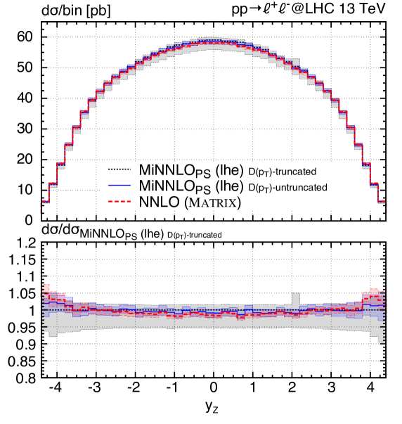
Figure 1: Rapidity distribution of the $Z$ boson. The plot compares the MiNNLO_PS prediction with untruncated (blue solid) and truncated (black dotted) $D({p_{\text{T}}})$ function at the LHE level with the NNLO prediction obtained with Matrix (red, dashed). The lower panel shows the ratio to the truncated prediction.

3.2 Evolution of parton densities and scale setting

As a second aspect that affects MiNNLO_PS predictions we discuss the evolution of parton densities at low scales. To ensure consistency of ${\mu_{\text{F}}}$ variations we would like to avoid truncating the PDFs at their own infrared cutoff $\Lambda_{\rm PDF}$, but rather carry out a consistent DGLAP evolution down to lower scales. By doing this, we do not aim for a physically accurate description of the ${p_{\text{T}}}$ spectrum below $\Lambda_{\rm PDF}$, but simply ensure that Eq. (2) can be evaluated all the way down to sufficiently small ${p_{\text{T}}}$, where it becomes vanishingly small due to the Sudakov suppression. This kinematic region will subsequently be corrected by the parton shower and hadronization process. As a consequence, several prescriptions can be formulated.

We read the PDFs (including the corresponding heavy quark thresholds) from the LHAPDF [11] package and build corresponding HOPPET grids [12], which facilitates an efficient evaluation of all convolutions with the coefficient functions. These HOPPET grids are a copy of the LHAPDF sets for ${\mu_{\text{F}}}\gtrsim\Lambda_{\rm PDF}$. Below this scale, we freeze the number of active flavours to those of the PDF set at ${\mu_{\text{F}}}=\Lambda_{\rm PDF}$, and we carry out a DGLAP evolution down to lower scales of ${\mu_{\text{F}}}\sim\Lambda$ using HOPPET. This prescription allows us to define a hybrid PDF set that can be evaluated consistently also for small values of ${\mu_{\text{F}}}\sim{p_{\text{T}}}$ with the desired numerical precision. For consistency, we adopt the same running coupling as that provided by the PDF set via LHAPDF, with the full heavy quark threshold information. The integral that defines the Sudakov form factor $\tilde{S}({p_{\text{T}}})$ given in Eq. (24) is then evaluated exactly in numerical form. This numerical prescription replaces the analytic formulae of $\tilde{S}({p_{\text{T}}})$ given in Ref. [4].

In the practical implementation of Ref. [4] we followed a prescription to smoothly turn off the contribution of $[D(p_{T})]^{(3)}$ in Eq. (2) at large ${p_{\text{T}}}$ by introducing modified logarithms

$$\ln\frac{Q}{{p_{\text{T}}}}\rightarrow L\equiv\frac{1}{p}\ln\left(1+\left(\frac{Q}{{p_{\text{T}}}}\right)^{p}\right)\,,$$ (10)

where $p$ is a free positive parameter. Larger values of $p$ correspond to logarithms that tend to zero at a faster rate at large ${p_{\text{T}}}$, while the limit ${p_{\text{T}}}\rightarrow 0$ remains unaffected. This prescription modifies Eq. (2) by terms beyond accuracy, and it has to be performed at the level of Eq. (2) in order to preserve the total derivative (hence the total cross section). This corresponds to:

• Setting the perturbative scales in the $D({p_{\text{T}}})$ (or $[D(p_{T})]^{(3)}$) function of Eq. (2) to

  $${\mu_{\text{R}}}=K_{\text{R}}\,Q\,e^{-L}\,,\qquad{\mu_{\text{F}}}=K_{\text{F}}\,Q\,e^{-L}\,.$$ (11)

• Changing the lower integration bound of the Sudakov (24) (the integrand is not modified directly) to

  $${p_{\text{T}}}\rightarrow Qe^{-L}.$$ (12)

• Multiply $D({p_{\text{T}}})$ (or $[D(p_{T})]^{(3)}$) by the following Jacobian factor:

  $$D({p_{\text{T}}})\rightarrow{\cal J}_{Q}D\left({p_{\text{T}}}\right),\qquad{\cal J}_{Q}\equiv\frac{\left(Q/{p_{\text{T}}}\right)^{p}}{1+\left(Q/{p_{\text{T}}}\right)^{p}}\,.$$ (13)

On the other hand, one has some freedom of setting the corresponding scales in the differential NLO cross section for ${\rm FJ}$ production in Eq. (2), as long as they tend to ${p_{\text{T}}}$ at small transverse momentum. We will discuss possible choices at the end of this section.

In Eq. (11), $K_{R,F}$ are scale variation parameters that are varied between $1/2$ and $2$ to estimate perturbative uncertainties. As a way of smoothly approaching non-perturbative scales at low ${p_{\text{T}}}$, we introduce the alternative scale setting

$${\mu_{\text{R}}}=K_{\text{R}}\,\left(Q\,e^{-L}+Q_{0}\,g({p_{\text{T}}})\right)\,,\qquad{\mu_{\text{F}}}=K_{\text{F}}\,\left(Q\,e^{-L}+Q_{0}\,g({p_{\text{T}}})\right),$$ (14)

where $g({p_{\text{T}}})$ is a damping function. The scale $Q_{0}$ is a non-perturbative parameter which has the role of regularising the Landau singularity and as such it should be tuned together with the hadronization model using experimental data. One has some freedom in choosing $g({p_{\text{T}}})$, and we explore the options

$$g({p_{\text{T}}})=1,\qquad g({p_{\text{T}}})=\frac{1}{1+\frac{Q}{Q_{0}}e^{-L}}\,.$$ (15)

The difference between the two is that the second option further suppresses the shift by $Q_{0}$ at large transverse momentum. This prescription is also consistently adopted in the Sudakov form factor $\tilde{S}({p_{\text{T}}})$, defined in Eq. (24), at the integrand level. The modified Sudakov is then evaluated exactly via a numerical calculation of the integral. As far as the $D({p_{\text{T}}})$ function is concerned, analogously to what has been discussed for the modified logarithms in Eq. (13), the choice in Eq. (14) requires the introduction of an additional factor ${\cal J}_{Q_{0}}$ (for the two choices in Eq. (15), respectively)

$${\cal J}_{Q_{0}}\equiv\frac{Q\,e^{-L}}{Q\,e^{-L}+Q_{0}}\,,\qquad{\cal J}_{Q_{0}}\equiv Q\,e^{-L}\frac{1-g^{2}({p_{\text{T}}})}{Q\,e^{-L}+Q_{0}\,g({p_{\text{T}}})}\,,$$ (16)

which multiplies only the derivative of the luminosity. This modifies Eq. (13) as

$${\cal J}_{Q}D({p_{\text{T}}})\rightarrow{\cal J}_{Q}\left(-\frac{\mathrm{d}\tilde{S}({p_{\text{T}}})}{\mathrm{d}{p_{\text{T}}}}{\cal L}({p_{\text{T}}})+{\cal J}_{Q_{0}}\frac{\mathrm{d}{\cal L}({p_{\text{T}}})}{\mathrm{d}{p_{\text{T}}}}\right)\,,$$ (17)

where the scales are set as in Eq. (14) after taking the derivatives in the right-hand-side of the above equation.

The scale $Q_{0}>\Lambda$ smoothly freezes the coupling and PDFs at low scales. We stress that this prescription does not affect the double logarithmic terms in $\tilde{S}({p_{\text{T}}})$, which ensures that Eq. (2) still vanishes exponentially for ${p_{\text{T}}}\rightarrow 0$. With this prescription to regularize the Landau pole, we can now integrate safely all the way down to ${p_{\text{T}}}$ scales at which the integrand vanishes, which is an essential requirement in order for Eq. (2) to be NNLO accurate. This is because the contribution of the total derivative to the integral over ${p_{\text{T}}}$ must vanish at the lower bound of integration. If this is not the case, one introduces an additional systematic uncertainty due to the truncation (or slicing) of the integral at scales where the integrand is not vanishingly small. In this respect the scale $Q_{0}$ is not a slicing parameter, as it simply acts by freezing the coupling and the PDFs in the infrared region. At the same time, this allows us to perform a consistent scale variation all the way down to ${p_{\text{T}}}=0$, which would not be the case if a slicing cutoff were introduced in the integral of Eq. (2). We do not find a visible difference between the two options in Eq. (15), and we therefore stick to the second of the two with $Q_{0}=2$ GeV as our default. We stress that, for differential distributions sensitive to infrared dynamics (for instance the transverse momentum of the $Z$ boson in the peak region), the $Q_{0}$ parameter must be determined together with a tune of the parton-shower hadronization model.

As a final step, we discuss the scale setting adopted in the NLO ${\rm FJ}$ cross section in Eq. (2). The default prescription in MiNLO^′ and MiNNLO_PS is to set the perturbative scales in this term to

$${\mu_{\text{R}}}=K_{\text{R}}\,{p_{\text{T}}}\,,\qquad{\mu_{\text{F}}}=K_{\text{F}}\,{p_{\text{T}}}\,,$$ (18)

or, if the smooth freezing is introduced, to

$${\mu_{\text{R}}}=K_{\text{R}}\,\left({p_{\text{T}}}+g({p_{\text{T}}})\,Q_{0}\right)\,,\qquad{\mu_{\text{F}}}=K_{\text{F}}\,\left({p_{\text{T}}}+g({p_{\text{T}}})\,Q_{0}\right)\,.$$ (19)

This ensures that in the small ${p_{\text{T}}}$ limit these scales match the ones used in the Sudakov form factor and the $D({p_{\text{T}}})$ function, which are constrained by the structure of ${p_{\text{T}}}$ resummation, hence guaranteeing a correct matching at small ${p_{\text{T}}}$. However, one can also choose to set the scales of the NLO calculation as in Eqs. (11) and (14), such that at large ${p_{\text{T}}}$ the scales of the MiNNLO_PS predictions are of the order of the invariant mass $Q$ of the colour singlet. We employ Eq. (14) in the results shown in this article. While this choice is more appropriate for inclusive observables, the one in Eq. (19) is preferable to obtain predictions in regimes where the colour singlet is produced with large ${p_{\text{T}}}$. Both options (14) and (19) are made available to the user.

3.3 Impact of shower recoil scheme on kinematics of the colour singlet

Another source of higher-order corrections in the final prediction is given by the parton shower. Shower simulations are expected to be accurate in configurations dominated by soft and/or collinear radiation. Away from these limits the corrections introduced by the shower evolution are subleading (higher order in nature) to the fixed-order description of the hard scattering process.

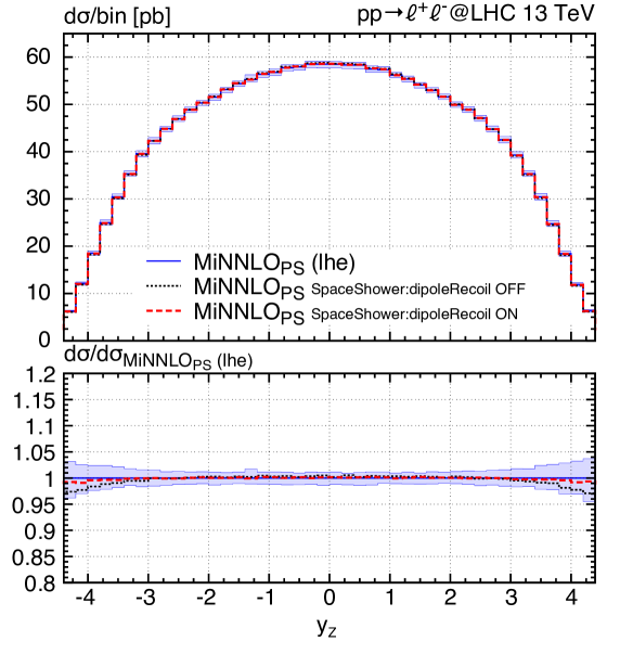
Figure 2: Rapidity distribution of the $Z$ boson. The plot compares MiNNLO_PS predictions at LHE level (blue, solid) and after showering using different recoil schemes in Pythia8 with the option SpaceShower:dipoleRecoil 0 (black, dotted) and SpaceShower:dipoleRecoil 1 (red, dashed). The lower panel shows the ratio to the prediction at LHE level.

As a consequence, the shower may lead to higher-order corrections to physical observables that one would naively expect to be largely insensitive to the showering process. As an example, let us consider again the rapidity distribution of the $Z$ boson. This inclusive quantity should be nearly independent of the infrared dynamics. However, if we compare MiNNLO_PS predictions for this quantity at the LHE level and after showering with Pythia8 [13] (without hadronization) in Fig. 2, we observe that the shower suppresses configurations where the vector boson is produced at large absolute rapidities. This effect can traced back to the default (black, dotted line in Fig. 2) shower recoil scheme used by Pythia8 for initial-state radiation, which is global, i.e. the recoil of a generated particle is shared among all particles in the final state of the event. Naturally, this affects also the kinematics of the $Z$ boson and it is responsible for the behaviour observed in Fig. 2.

This observation can be confirmed by choosing an alternative recoil scheme. In a large-$N_{c}$ picture, one can for instance share the recoil globally only for emissions off initial–initial colour dipoles, while assigning it locally (i.e. entirely taken from a single final state particle) for emissions off initial–final colour dipoles (i.e. a colour line that connects an initial-state and a final-state particle). This scheme is available within Pythia8 via the flag SpaceShower:dipoleRecoil 1 (cf. Ref. [14] for details). In this case, we expect the $Z$ boson to be less affected by the parton shower than in the default recoil scheme. As an example let us consider the leading order configuration $q+\bar{q}\rightarrow Z$. If the quark lines emit a real gluon ($q+\bar{q}\rightarrow Z+g$), the recoil is taken from the $Z$ boson. One then is left with two initial–final and no initial–initial colour dipoles. As a consequence, the emission of an additional radiation will never affect the kinematics of the $Z$ boson. Conversely, an extra radiation from the $q+g\rightarrow Z+q$ configuration will affect the $Z$ boson if it is emitted off the initial-state $qg$ dipole. From the plot we indeed observe that this less global version of the recoil scheme (red, dashed line in Fig. 2) impacts the $Z$-boson kinematics very mildly.

We stress that the effects of the shower recoil scheme on the rapidity distribution are by all means subleading and formally beyond NNLO accuracy. On the other hand, the choice of the recoil scheme can have consequences for the logarithmic accuracy of a parton shower [15, 16, 17], which implies that a comprehensive discussion about a given scheme must take place in this context. Specifically, the alternative recoil scheme that we have just discussed may arguably have consequences for the description of the transverse-momentum distribution of the $Z$ boson, which in this scheme becomes insensitive to some of the radiation emitted off the initial-state quarks. In a transverse-momentum ordered shower like Pythia8, this may result in next-to-leading logarithmic contributions to the $Z$ transverse-momentum spectrum being potentially mistreated (cf. Ref. [16] for details). Since in this article we assume parton showers to be LL accurate, this problem is strictly of subleading nature. However, recent progress in formulating NLL accurate parton showers [18, 19] raises the question of whether the MiNNLO_PS method (in fact any of the available NNLO+PS methods [1, 2, 3, 4]) preserves the shower accuracy after matching. A study of this type is beyond the scope of this article and left for future work.

As far as the matching to NNLO QCD for the $2\rightarrow 1$ processes studied in this paper is concerned, we use the option SpaceShower:dipoleRecoil 1 as the default for our results so that shower effects on inclusive quantities are minimised.

4 Results for Drell Yan and Higgs boson production

In this section we compare the NNLO+PS predictions obtained with MiNNLO_PS to f NNLO results obtained with the public code Matrix [9]. We consider the processes

$$pp\rightarrow\ell^{+}\ell^{-}\,,\quad pp\rightarrow\ell^{-}\bar{\nu}_{\ell}\,,\quad pp\rightarrow\ell^{+}\nu_{\ell}\,,\quad{\rm and}\quad pp\rightarrow H\,,$$ (20)

for massless leptons $\ell\in\{e,\mu\}$. The Higgs is produced on-shell in the heavy-top approximation, while for the DY processes the full off-shell effects are taken into account, including $Z$-boson, $W$-boson, and photon ($\gamma^{*}$) contributions. For neutral-current DY we restrict the invariant mass of dilepton pair to the $Z$-mass window

$$66~{}{\rm GeV}\leq M_{\ell^{+}\ell^{-}}\leq 116~{}{\rm GeV}\,$$ (21)

to avoid the photon singularity.

We consider 13 TeV LHC collisions. For the EW parameters we employ the $G_{\mu}$ scheme with the EW mixing angles given by $\cos^{2}\theta_{\tiny{\mbox{W}}}=m_{W}{}^{2}/m_{Z}{}^{2}$ and $\alpha=\sqrt{2}\,G_{\mu}m_{W}{}^{2}\sin^{2}\theta_{\tiny{\mbox{W}}}/\pi$. The following values are used as input parameters: $G_{\tiny{\mbox{F}}}=1.16639\times 10^{-5}$ GeV^-2, $m_{W}{}=80.385$ GeV, $\Gamma_{W}=2.0854$ GeV, $m_{Z}=91.1876$ GeV, $\Gamma_{Z}=2.4952$ GeV, and ${m_{\text{H}}}{}=125$ GeV. With an on-shell top-quark mass of $m_{t}=173.2$ GeV and $n_{f}=5$ massless quark flavours, we use the corresponding NNLO PDF set with $\alpha_{\mathrm{S}}(m_{Z}{})=0.118$ of NNPDF3.1 [10] for the DY results and the set PDF4LHC15_nnlo_mc of PDF4LHC15 [20, 21, 22, 23] for Higgs boson production.

The reference f NNLO results of Matrix have been obtained by setting the central scales to the invariant mass of the produced color singlet, i.e.

$${\mu_{\text{R}}}={\mu_{\text{F}}}=Q,\,\qquad Q=M_{\ell^{+}\ell^{-}},M_{\ell^{-}\bar{\nu}_{\ell}},M_{\ell^{+}\nu_{\ell}},m_{H}\,,$$ (22)

while the MiNNLO_PS simulations are obtained using the default setup discussed in Section 3. Scale uncertainties are obtained by varying the renormalisation and factorisation scales by a factor of two about their central value while keeping $1/2\leq{\mu_{\text{R}}}/{\mu_{\text{F}}}\leq 2$. All MiNNLO_PS results are showered with Pythia8 [13], switching off hadronization and underlying event. In all of the results that follow, the NNLO prediction of Matrix is represented by a red, dashed curve with a red band, while the MiNNLO_PS prediction is shown in blue, solid.

4.1 Neutral-current and charged-current Drell Yan production

Process	NNLO (Matrix)	MiNNLOPS	Ratio
$pp\rightarrow\ell^{+}\ell^{-}$	$\;\,1919(1)_{-1.1\%}^{+0.8\%}$ pb	$\;\,1926(1)_{-1.1\%}^{+1.4\%}$ pb	1.004
$pp\rightarrow\ell^{-}\bar{\nu}_{\ell}$	$\;\,8626(4)_{-1.2\%}^{+1.0\%}$ pb	$\;\,8689(4)_{-1.5\%}^{+1.7\%}$ pb	1.007
$pp\rightarrow\ell^{+}\nu_{\ell}$	$11677(5)_{-1.3\%}^{+0.9\%}$ pb	$11755(5)_{-1.6\%}^{+1.5\%}$ pb	1.007

Table 1: Total cross sections of the Drell Yan production processes. The number in brackets denotes the numerical uncertainty on the last digit.

We start by discussing the total production rates of the DY processes, reported in Table 1. We observe an excellent agreement between the NNLO QCD prediction and the MiNNLO_PS result, which are consistent at the few-permille level. We stress again that the two calculations use different scale settings and are therefore expected to differ by effects beyond NNLO. As one can see from Table 1, these differences are small and the central prediction of each calculation lies within the perturbative uncertainty of the other. Moreover, we observe that the MiNNLO_PS calculation features a slightly larger scale uncertainty. This is due to the more conservative uncertainty prescription adopted in the MiNNLO_PS case, which involves varying the renormalisation scale ${\mu_{\text{R}}}$ also in the Sudakov form factor $\tilde{S({p_{\text{T}}})}$, defined in Eq. (24). This choice better reflects the perturbative uncertainty associated with the MiNNLO_PS matching procedure.

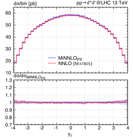
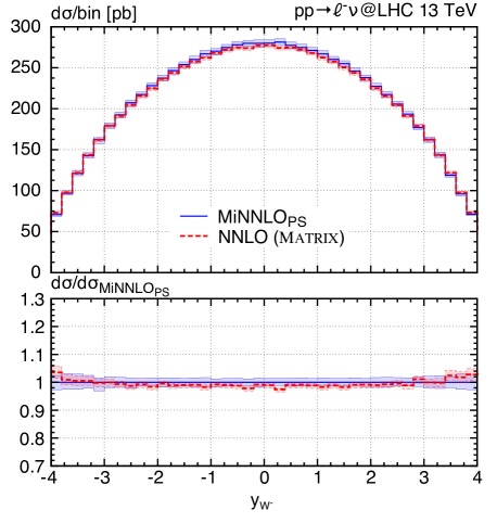
Figure 3: The rapidity distribution of the leptonic pair in neutral- (left plot) and charged-current (right plot) Drell Yan production. The lower panel shows the ratio of the NNLO and the MiNNLO_PS predictions to the latter.

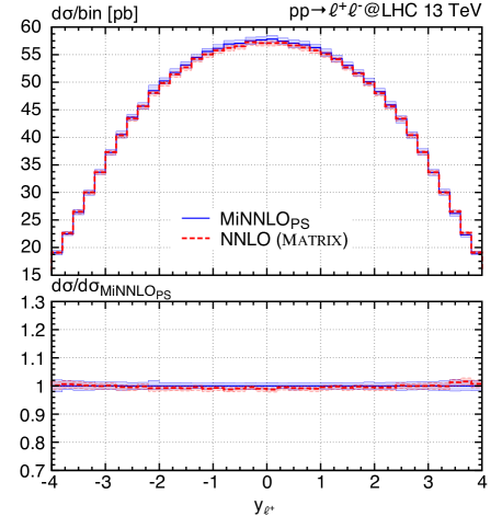
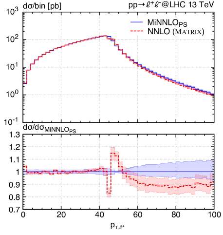
Figure 4: Rapidity distribution (left) and transverse momentum (right) of the positively charged lepton in neutral-current Drell Yan production. The lower panel shows the ratio to the MiNNLO_PS prediction.

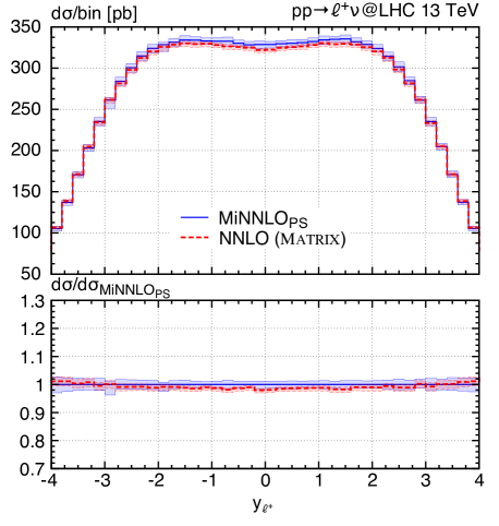
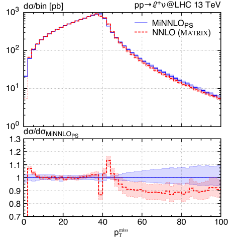
Figure 5: Rapidity distribution of the charged lepton (left) and missing transverse momentum (right) in charged-current Drell Yan production. The lower panel shows the ratio to the MiNNLO_PS prediction.

We continue by considering the rapidity distribution of the leptonic system in $Z$/$\gamma^{*}$ and $W^{-}$ production, shown in Fig. 3. The considerations made above for the inclusive cross section hold in this case as well, and we observe a very good agreement between the MiNNLO_PS and the f NNLO predictions across the entire spectrum, with moderately larger perturbative uncertainties in the MiNNLO_PS case. In comparison to the $Z$ rapidity distribution presented in Ref. [4], we observe that the shape of the new MiNNLO_PS result is much closer to the f NNLO prediction in the forward rapidity region. Each of the aspects discussed in this article (reduced difference due to higher-order terms with respect to f NNLO, improved evolution of the PDFs and scale setting, choice of the shower recoil scheme) plays a role in this improvement, as discussed in the previous section.

Finally, we show a sample of kinematic distribution of the final-state leptons. For neutral-current DY production we compare MiNNLO_PS to f NNLO predictions for the rapidity distribution and the transverse-momentum distribution of the positively charged lepton in Fig. 4. Similarly, in the case of $W^{+}$ production we show the same comparison for the missing transverse-momentum distribution and for the rapidity distribution of the charged lepton in Fig 5. We observe a very good agreement between the two calculations for the rapidity distributions, and for the region of the transverse-momentum spectrum insensitive to shower effects. Conversely, the parton shower provides an improved description for $p_{\rm T,\ell^{+}}~{}(p_{\rm T}^{\rm miss})\lesssim 5$ GeV and $p_{\rm T,\ell^{+}}~{}(p_{\rm T}^{\rm miss})\gtrsim m_{V}/2$ where the cross section is sensitive to multi particle emissions and therefore receives relevant corrections from the parton shower that resums integrable, but large logarithmic terms. The perturbative instability at the threshold is a well known feature of fixed-order calculations [25]. It appears at $p_{\rm T,\ell^{+}}~{}(p_{\rm T}^{\rm miss})\sim m_{V}/2$, since at LO, where the leptons are back-to-back and can share only the available partonic centre-of-mass energy $\sqrt{\hat{s}}=Q$, the distribution is kinematically restricted to the region $p_{\rm T,\ell^{+}}~{}(p_{\rm T}^{\rm miss})\leq Q/2$ and on-shell configurations $Q\sim m_{V}$ provide by far the dominant contribution. The region $p_{\rm T,\ell^{+}}~{}(p_{\rm T}^{\rm miss})\gtrsim m_{V}/2$ is filled only upon inclusion of higher-order corrections, and the NNLO predictions becomes effectively only NLO accurate, as indicated by the enlarged uncertainty bands.

4.2 Higgs boson production

Process	NNLO (Matrix)	MiNNLOPS	ratio
$pp\rightarrow H$	$39.64(1)_{-10.4\%}^{+10.7\%}$ pb	$38.03(2)_{-9.0\%}^{+10.2\%}$ pb	0.960

Table 2: Total cross sections of Higgs-boson production. The number in brackets denotes the numerical uncertainty on the last digit.

Table 2 gives the inclusive Higgs cross section at f NNLO computed with Matrix and the one obtained with the MiNNLO_PS generator. As in the case of DY production, we observe a good agreement between the two predictions that are well compatible within the quoted scale uncertainties, and they are closer than in the original setup of Ref. [4]. The moderate numerical difference between the two results is due to the different scale settings in the two calculations.

The rapidity distribution of the Higgs boson is shown in the left plot of Fig. 6. The MiNNLO_PS and NNLO predictions are in mutually good agreement within the perturbative uncertainties. The right plot of Fig. 6 shows the Higgs transverse-momentum distribution. This observable displays the effect of the MiNNLO_PS scale setting in Eq. (14) compared to the one in the Matrix computation in Eq. (22). The two scales differ significantly at low and moderate transverse momenta, while they become identical at large transverse momentum $p_{\rm T,H}\gtrsim m_{H}$, where the MiNNLO_PS and Matrix predictions are in full agreement. We recall that the scales of the differential NLO cross section for ${\rm FJ}$ production in Eq. (2) can also be set to the transverse momentum as in Eq. (19). This choice, used in the original publication [4], is more appropriate in regimes where the Higgs boson (or the accompanying QCD jets) are produced with large transverse momentum.

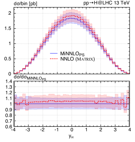
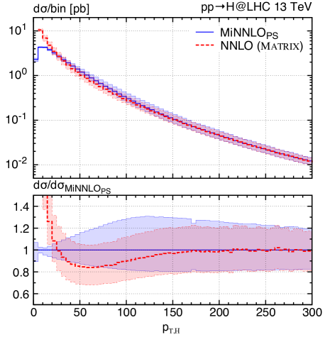
Figure 6: The rapidity distribution of the Higgs boson (left) and its transverse momentum (right). The lower panel shows the ratio of the NNLO and the MiNNLO_PS predictions to the latter.

5 Conclusions

In this article we have addressed a number of aspects of the MiNNLO_PS method, which combines NNLO QCD calculations with parton-shower simulations. As a case study we have considered the production of a colour-singlet final state in $2\rightarrow 1$ reactions at the LHC.

We have identified the main sources of differences between the MiNNLO_PS prediction and f NNLO calculations, which are due to corrections beyond accuracy introduced in the matching procedure. A number of prescriptions has been presented to either remove or reduce the impact of such corrections in the MiNNLO_PS results, specifically:

• The MiNNLO_PS formula has been refined to include additional terms at all orders in the matching procedure that reduce the subleading differences between MiNNLO_PS and f NNLO calculations.

• The evolution of the parton densities at small transverse momentum has been improved, and the scale setting in the coupling and PDFs has been consistently adjusted so that at large transverse momentum it matches that of the f NNLO calculation.

• We studied the impact of the parton-shower recoil scheme on the kinematics of the colour singlet, and discussed how this dependence can be reduced.

The new prescriptions for the MiNNLO_PS matching procedure have been used to obtain updated predictions for Higgs, charged- and neutral-current Drell Yan production, finding a significantly improved agreement between the MiNNLO_PS and f NNLO calculations for inclusive observables, with commensurate scale uncertainties.

The prescriptions presented in this article do not affect the performance of the MiNNLO_PS method in terms of efficiency and speed. The generation of fully exclusive NNLO+PS events is merely $50\%$ slower than the corresponding MiNLO^′ calculation. The codes to obtain the results presented in this article are released within the POWHEG-BOX framework.

Acknowledgements. We would like to thank Paolo Nason and Giulia Zanderighi for useful discussions and constructive comments on the manuscript. We also wish to thank Luca Rottoli for providing us with a toy set of parton distributions with a low cutoff that we used to validate our PDF evolution at low factorisation scales.

Appendix A Explicit formulae for the evaluation of $D({p_{\text{T}}})$

In this section we supplement the formulae given in Ref. [4] with the ones required to calculate the untruncated variant of the function $[D({p_{\text{T}}})]^{(3)}$ given in Eq. (9). The luminosity factor is defined as as [4]

$${\cal L}({p_{\text{T}}}) =\sum_{c,c^{\prime}}\frac{\mathrm{d}|M^{\scriptscriptstyle\rm F}|_{cc^{\prime}}^{2}}{\mathrm{d}\Phi_{\scriptscriptstyle\rm F}}\sum_{i,j}\bigg{\{}\left(\tilde{C}^{[a]}_{ci}\otimes f_{i}^{[a]}\right)\tilde{H}({p_{\text{T}}})\left(\tilde{C}^{[b]}_{c^{\prime}j}\otimes f_{j}^{[b]}\right)+\left(G^{[a]}_{ci}\otimes f_{i}^{[a]}\right)\tilde{H}({p_{\text{T}}})\left(G^{[b]}_{c^{\prime}j}\otimes f_{j}^{[b]}\right)\bigg{\}}\,.$$ (23)

Here $M^{\scriptscriptstyle\rm F}$ is the Born matrix element for the production of the colour singlet ${\rm F}$, and $f$ denotes the parton distribution functions. Moreover, $\tilde{H}$ encodes the virtual corrections to this process up to two loops, and $\tilde{C}$ and $G$ are the coefficient functions up to ${\cal O}(\alpha_{\mathrm{S}}^{2})$ (see Ref. [4] for details). The Sudakov form factor $\tilde{S}({p_{\text{T}}})$ is defined as

$$\tilde{S}({p_{\text{T}}})=2\int_{{p_{\text{T}}}}^{Q}\frac{\mathrm{d}q}{q}\left(A(\alpha_{\mathrm{S}}(q))\ln\frac{Q^{2}}{q^{2}}+\tilde{B}(\alpha_{\mathrm{S}}(q))\right),$$ (24)

with

$$A(\alpha_{\mathrm{S}})= \left(\frac{\alpha_{\mathrm{S}}}{2\pi}\right)A^{(1)}+\left(\frac{\alpha_{\mathrm{S}}}{2\pi}\right)^{2}A^{(2)}+\left(\frac{\alpha_{\mathrm{S}}}{2\pi}\right)^{3}A^{(3)}\,,$$

$$\tilde{B}(\alpha_{\mathrm{S}})= \left(\frac{\alpha_{\mathrm{S}}}{2\pi}\right)B^{(1)}+\left(\frac{\alpha_{\mathrm{S}}}{2\pi}\right)^{2}\tilde{B}^{(2)}\,,$$ (25)

and its derivative reads

$$\frac{\mathrm{d}\tilde{S}({p_{\text{T}}})}{\mathrm{d}{p_{\text{T}}}}=-\frac{2}{{p_{\text{T}}}}\left(A(\alpha_{\mathrm{S}}({p_{\text{T}}}))\ln\frac{Q^{2}}{{p_{\text{T}}}^{2}}+\tilde{B}(\alpha_{\mathrm{S}}({p_{\text{T}}}))\right)\,.$$ (26)

All coefficients of the above equations are defined in Section 4 and Appendix B of Ref. [4], including their scale dependence. The above formulae are inserted into Eq. (9), where the derivative of ${\cal L}({p_{\text{T}}})$ is evaluated numerically to ensure that the exact total derivative in Eq. (2) that we started our derivation from is not modified. The numerical derivative of ${\cal L}({p_{\text{T}}})$ is performed by evaluating Eq. (23) using a five-point stencil discrete derivative calculated on a fine grid around ${p_{\text{T}}}$.

One last necessary ingredient is given by the first and second order expansion of $D({p_{\text{T}}})$ in powers of $\alpha_{\mathrm{S}}({p_{\text{T}}})$. Its coefficients read

$$[D({p_{\text{T}}})]^{(1)} =-\left[\frac{\mathrm{d}\tilde{S}({p_{\text{T}}})}{\mathrm{d}{p_{\text{T}}}}\right]^{(1)}[{\cal L}({p_{\text{T}}})]^{(0)}+\left[\frac{\mathrm{d}{\cal L}({p_{\text{T}}})}{\mathrm{d}{p_{\text{T}}}}\right]^{(1)},$$

$$[D({p_{\text{T}}})]^{(2)} =-\left[\frac{\mathrm{d}\tilde{S}({p_{\text{T}}})}{\mathrm{d}{p_{\text{T}}}}\right]^{(2)}[{\cal L}({p_{\text{T}}})]^{(0)}-\left[\frac{\mathrm{d}\tilde{S}({p_{\text{T}}})}{\mathrm{d}{p_{\text{T}}}}\right]^{(1)}[{\cal L}({p_{\text{T}}})]^{(1)}+\left[\frac{\mathrm{d}{\cal L}({p_{\text{T}}})}{\mathrm{d}{p_{\text{T}}}}\right]^{(2)},$$ (27)

where

$$\left[\frac{\mathrm{d}\tilde{S}({p_{\text{T}}})}{\mathrm{d}{p_{\text{T}}}}\right]^{(1)} =-\frac{2}{{p_{\text{T}}}}\left(A^{(1)}\ln\frac{Q^{2}}{{p_{\text{T}}}^{2}}+B^{(1)}\right)\,,$$

$$\left[\frac{\mathrm{d}\tilde{S}({p_{\text{T}}})}{\mathrm{d}{p_{\text{T}}}}\right]^{(2)} =-\frac{2}{{p_{\text{T}}}}\left(A^{(2)}\ln\frac{Q^{2}}{{p_{\text{T}}}^{2}}+\tilde{B}^{(2)}\right)\,,$$

$$[{\cal L}({p_{\text{T}}})]^{(0)} =\sum_{c,c^{\prime}}\frac{\mathrm{d}|M^{\scriptscriptstyle\rm F}|_{cc^{\prime}}^{2}}{\mathrm{d}\Phi_{\rm B}}\,f_{c}^{[a]}f_{c^{\prime}}^{[b]}\,,$$

$$[{\cal L}({p_{\text{T}}})]^{(1)} =\sum_{c,c^{\prime}}\frac{\mathrm{d}|M^{\scriptscriptstyle\rm F}|_{cc^{\prime}}^{2}}{\mathrm{d}\Phi_{\rm B}}\bigg{\{}H^{(1)}f_{c}^{[a]}f_{c^{\prime}}^{[b]}+(C^{(1)}\otimes f)_{c}^{[a]}f_{c^{\prime}}^{[b]}+f_{c}^{[a]}(C^{(1)}\otimes f)_{c^{\prime}}^{[b]}\bigg{\}}\,,$$

$$\left[\frac{\mathrm{d}{\cal L}({p_{\text{T}}})}{\mathrm{d}{p_{\text{T}}}}\right]^{(1)} =\sum_{c,c^{\prime}}\frac{\mathrm{d}|M^{\scriptscriptstyle\rm F}|_{cc^{\prime}}^{2}}{\mathrm{d}\Phi_{\rm B}}\frac{2}{{p_{\text{T}}}}\bigg{\{}(\hat{P}^{(0)}\otimes f)_{c}^{[a]}f_{c^{\prime}}^{[b]}+f_{c}^{[a]}(\hat{P}^{(0)}\otimes f)_{c^{\prime}}^{[b]}\bigg{\}}\,,$$

$$\left[\frac{\mathrm{d}{\cal L}({p_{\text{T}}})}{\mathrm{d}{p_{\text{T}}}}\right]^{(2)} =\sum_{c,c^{\prime}}\frac{\mathrm{d}|M^{\scriptscriptstyle\rm F}|_{cc^{\prime}}^{2}}{\mathrm{d}\Phi_{\rm B}}\frac{2}{{p_{\text{T}}}}\bigg{\{}(\hat{P}^{(1)}\otimes f)_{c}^{[a]}f_{c^{\prime}}^{[b]}+f_{c}^{[a]}(\hat{P}^{(1)}\otimes f)_{c^{\prime}}^{[b]}$$

$$+H^{(1)}\left[(\hat{P}^{(0)}\otimes f)_{c}^{[a]}f_{c^{\prime}}^{[b]}+f_{c}^{[a]}(\hat{P}^{(0)}\otimes f)_{c^{\prime}}^{[b]}\right]$$

$$+(C^{(1)}\otimes f)_{c}^{[a]}(\hat{P}^{(0)}\otimes f)_{c^{\prime}}^{[b]}+(\hat{P}^{(0)}\otimes f)_{c}^{[a]}(C^{(1)}\otimes f)_{c^{\prime}}^{[b]}$$

$$+f_{c}^{[a]}(\hat{P}^{(0)}\otimes C^{(1)}\otimes f)_{c^{\prime}}^{[b]}+(\hat{P}^{(0)}\otimes C^{(1)}\otimes f)_{c}^{[a]}f_{c^{\prime}}^{[b]}$$

$$-2\beta_{0}\pi\Big{[}H^{(1)}f_{c}^{[a]}f_{c^{\prime}}^{[b]}+(C^{(1)}\otimes f)_{c}^{[a]}f_{c^{\prime}}^{[b]}+f_{c}^{[a]}(C^{(1)}\otimes f)_{c^{\prime}}^{[b]}\Big{]}\bigg{\}}\,.$$ (28)

The scale dependence is implemented as in Appendix D of Ref. [4], and in addition the above $[D({p_{\text{T}}})]^{(1)}$ and $[D({p_{\text{T}}})]^{(2)}$ terms depend on the renormalisation and factorisation scale factors $K_{\text{R}}$ and $K_{\text{F}}$ as

$$[D({p_{\text{T}}})]^{(1)}(K_{\text{F}},K_{\text{R}}) =[D({p_{\text{T}}})]^{(1)}\,,$$

$$[D({p_{\text{T}}})]^{(2)}(K_{\text{F}},K_{\text{R}}) =[D({p_{\text{T}}})]^{(2)}-2\beta_{0}\pi\left[\frac{\mathrm{d}{\cal L}({p_{\text{T}}})}{\mathrm{d}{p_{\text{T}}}}\right]^{(1)}\ln\frac{K_{\text{F}}^{2}}{K_{\text{R}}^{2}}\,.$$ (29)

References

- Hamilton et al. [2013] K. Hamilton, P. Nason, C. Oleari, and G. Zanderighi, JHEP 05, 082 (2013), arXiv:1212.4504 [hep-ph] .
- Alioli et al. [2014] S. Alioli, C. W. Bauer, C. Berggren, F. J. Tackmann, J. R. Walsh, and S. Zuberi, JHEP 06, 089 (2014), arXiv:1311.0286 [hep-ph] .
- Höche et al. [2015] S. Höche, Y. Li, and S. Prestel, Phys. Rev. D91, 074015 (2015), arXiv:1405.3607 [hep-ph] .
- Monni et al. [2019] P. F. Monni, P. Nason, E. Re, M. Wiesemann, and G. Zanderighi, (2019), arXiv:1908.06987 [hep-ph] .
- Nason [2004] P. Nason, JHEP 11, 040 (2004), arXiv:hep-ph/0409146 [hep-ph] .
- Bahr et al. [2008] M. Bahr et al., Eur. Phys. J. C58, 639 (2008), arXiv:0803.0883 [hep-ph] .
- Frixione et al. [2007] S. Frixione, P. Nason, and C. Oleari, JHEP 11, 070 (2007), arXiv:0709.2092 [hep-ph] .
- Alioli et al. [2010] S. Alioli, P. Nason, C. Oleari, and E. Re, JHEP 06, 043 (2010), arXiv:1002.2581 [hep-ph] .
- Grazzini et al. [2018] M. Grazzini, S. Kallweit, and M. Wiesemann, Eur. Phys. J. C78, 537 (2018), arXiv:1711.06631 [hep-ph] .
- Ball et al. [2017] R. D. Ball et al. (NNPDF), Eur. Phys. J. C 77, 663 (2017), arXiv:1706.00428 [hep-ph] .
- Buckley et al. [2015] A. Buckley, J. Ferrando, S. Lloyd, K. Nordström, B. Page, M. Rüfenacht, M. Schönherr, and G. Watt, Eur. Phys. J. C75, 132 (2015), arXiv:1412.7420 [hep-ph] .
- Salam and Rojo [2009] G. P. Salam and J. Rojo, Comput. Phys. Commun. 180, 120 (2009), arXiv:0804.3755 [hep-ph] .
- Sjöstrand et al. [2015] T. Sjöstrand, S. Ask, J. R. Christiansen, R. Corke, N. Desai, P. Ilten, S. Mrenna, S. Prestel, C. O. Rasmussen, and P. Z. Skands, Comput. Phys. Commun. 191, 159 (2015), arXiv:1410.3012 [hep-ph] .
- Cabouat and Sjöstrand [2018] B. Cabouat and T. Sjöstrand, Eur. Phys. J. C 78, 226 (2018), arXiv:1710.00391 [hep-ph] .
- Nagy and Soper [2010] Z. Nagy and D. E. Soper, JHEP 03, 097 (2010), arXiv:0912.4534 [hep-ph] .
- Dasgupta et al. [2018] M. Dasgupta, F. A. Dreyer, K. Hamilton, P. F. Monni, and G. P. Salam, JHEP 09, 033 (2018), arXiv:1805.09327 [hep-ph] .
- Bewick et al. [2020] G. Bewick, S. Ferrario Ravasio, P. Richardson, and M. H. Seymour, JHEP 04, 019 (2020), arXiv:1904.11866 [hep-ph] .
- Dasgupta et al. [2020] M. Dasgupta, F. A. Dreyer, K. Hamilton, P. F. Monni, G. P. Salam, and G. Soyez, (2020), arXiv:2002.11114 [hep-ph] .
- Forshaw et al. [2020] J. R. Forshaw, J. Holguin, and S. Plätzer, (2020), arXiv:2003.06400 [hep-ph] .
- Butterworth et al. [2016] J. Butterworth et al., J. Phys. G43, 023001 (2016), arXiv:1510.03865 [hep-ph] .
- Ball et al. [2015] R. D. Ball et al. (NNPDF), JHEP 04, 040 (2015), arXiv:1410.8849 [hep-ph] .
- Harland-Lang et al. [2015] L. A. Harland-Lang, A. D. Martin, P. Motylinski, and R. S. Thorne, Eur. Phys. J. C75, 204 (2015), arXiv:1412.3989 [hep-ph] .
- Dulat et al. [2016] S. Dulat, T.-J. Hou, J. Gao, M. Guzzi, J. Huston, P. Nadolsky, J. Pumplin, C. Schmidt, D. Stump, and C. P. Yuan, Phys. Rev. D93, 033006 (2016), arXiv:1506.07443 [hep-ph] .
- Nason and Oleari [2013] P. Nason and C. Oleari, (2013), arXiv:1303.3922 [hep-ph] .
- Catani and Webber [1997] S. Catani and B. Webber, JHEP 10, 005 (1997), arXiv:hep-ph/9710333 .