Physical-Layer Authentication Using Channel State Information and Machine Learning

Abstract

Strong authentication in an interconnected wireless environment continues to be an important, but sometimes elusive goal. Research in physical-layer authentication using channel features holds promise as a technique to improve network security for a variety of devices. We propose the use of machine learning and measured multiple-input multiple-output communications channel information to make a decision on whether or not to authenticate a particular device. This work analyzes the use of received channel state information from the wireless environment and demonstrates the employment of a generative adversarial neural network (GAN) trained with received channel data to authenticate a transmitting device. We compared a variety of machine learning techniques and found that the local outlier factor (LOF) algorithm reached 100% accuracy at lower signal to noise ratios (SNR) than other algorithms. However, before LOF reached 100%, we also show that the GAN was more accurate at lower SNR levels.

I Introduction

The protection of integrity, confidentiality, and availability is a challenge in wireless networks. Unlike networks with wired point-to-point connections, the broadcast nature of the wireless domain grants bona fide users and malicious actors the same access to the communication channel. As modern and future mobile networks bring the promise of very high data rate mobile communications, they must also be secure. Without appropriate security, there will be intrusions and attacks, countering the networks’ benefits.

Our ultimate intent is to classify a transmitter as either trusted or untrusted and use that information to make a decision on whether or not to authenticate. Machine learning tools have shown success at producing solutions for complex problems where data is consistently changing and difficult to characterize with simpler techniques [1]. To this end, we require unique transmitter features realized in the physical-layer environment.

The literature proposes two broad categories to distinguish legitimate from illegitimate devices at the physical-layer. The first relies on unique imperfections of the transmitter hardware that manifest as radio frequency (RF) fingerprints or signatures [2, 3, 4]. The second method leverages the stochastic nature of the wireless channel to take advantage of multi-path fading environments. The temporally and spatially-unique impulse or frequency response can be used to identify the transmitter [5, 6, 7].

Our proposed method is based on research using the second category. The effects of the multipath channel can be described in the channel state information (CSI) matrix. The focus of this paper is on the static case, and using a technique as described by [8] can be adopted to account for scenarios where motion is expected to change the CSI.

In this paper we use a generative adversarial network (GAN) to determine if a transmitter should be authenticated or denied access.

The contributions of this paper are:

• We retain both magnitude and phase information to make an authentication decision.

• We introduce analysis and simulation illustrating how the received CSI matrix elements and measurement error can be used for physical-layer authentication.

• There are two novel contributions in this work:

  (1) In Section III, a hypothesis test for physical-layer authentication using all elements in a CSI matrix and the respective receiver measurement error on those elements.

  (2) In Section V, the use of a GAN model to accurately use MIMO CSI as a basis of authentication at the physical-layer without requiring a survey of CSI at various positions.

• Our proposal discards the generative model at the conclusion of training and retains the discriminative model. The fully-trained discriminative model, having learned from a generative model that creates indistinguishably realistic CSI samples, is particularly suited to make authentication decisions.

This paper discusses previous work in physical-layer authentication using machine learning in Section II. Section III provides the concept for authentication using CSI and introduces a method to accomplish this. Next we present the system model for the GAN in Section IV. The development of the GAN and simulation results is shown in Section V. Finally, we summarize our observations and discuss future work in Section VI. With respect to notation, unless otherwise addressed, vectors are indicated with bold lower-case letters, and matrices are bold upper-case letters.

II Background and Related Work

This section introduces the channel model and discusses related work with machine learning, including the application of GANs.

II-A Channel model

The nature of the wireless medium affects the transmitted signal as it propagates to the receiver. The narrowband model of the wireless channel is given by

$${\textbf{{y}}=\textbf{{H}}\textbf{{x}}+\textbf{{n}}}$$ (1)

where y is the received signal, x is the transmitted signal, H is the time-varying CSI or channel response, and n is the noise vector. H is an ${N\times M}$ matrix of circularly symmetric complex-valued Gaussian random variables representing multiple channel conditions such as multi-path fading and the use of multiple antennas [9]. The number of transmitter antennas is $M$ and the number of receiver antennas is $N$. Each complex element within H is composed of real and imaginary zero-mean independent Gaussian random variables with identical variance and with Rayleigh distributed magnitude for NLOS scenarios. Jakes’ uniform scattering model [10] states that antennas spatially separated more than two carrier wavelengths from each other will observe sufficiently independent fading channels due to rapid decorrelation of the signal envelope among receivers.

II-B CSI authentication through machine learning

Many works have been conducted with machine learning and location information to make an authentication decision based on CSI [11, 12, 13, 14, 15, 16]. Support vector machines (SVM), K-means clustering, and an algorithm to determine temporal correlation of CSI magnitude were used by Liu et al. in [11]. In [12], Liao et al. used a convolutional neural network (CNN) to identify the valid users from attackers, based on a training dataset that included different path delays among the various users. Wang et al. [13] also used this methodology, but included a recurrent neural network (RNN), a hybrid CNN-RNN architecture, and a skip-layer CNN. In [14] and [15], Liao et al. again used a variety of neural networks to identify valid users and spoofers using pre-built training sets created by obtaining CSI from legitimate and illegal sensor node locations. In [16], Abyaneh et al. also used a CNN trained on pre-mapped transmitter locations in order to grant authentication, however, they also included the complex value of the CSI element as input to their neural network.

To implement many proposals, researchers pre-processed collected raw CSI and used the magnitude of the CSI elements, $|h_{n,m}|$, in their implementations. Additionally, those that use neural networks used training data that required advance knowledge of CSI between a monitor and possible legitimate and illegitimate transmitters positions. Our proposal retains the complex elements of the CSI to retain a rich set of features and our methodology does not need a priori CSI samples from an attacker’s position while we make use of unsupervised machine learning to reach an authentication decision.

Supervised learning through neural networks have helped to make advancements in a variety of fields and require training data to respond well when tested. If the task is for classification, training examples enable the network to accurately label subsequent samples. However, there are machine learning algorithms that are designed to detect outliers or anomalies.

II-C Machine learning for outlier and anomaly detection

There is broad use for detection systems that identify samples with features outside of the expected. A one-class machine learning problem trains on data from a single class, and during testing the tool will provide an output recognizing new samples as either inliers of the statistical distribution or outliers.

Local outlier factor (LOF) from Breunig et al. in [17] quantifies the relative degree of isolation of a sample to its neighbors. For samples with density similar to that of the local cluster, the LOF value approaches 1. Inlier samples with higher density than their neighbors have a LOF less than 1, and outliers have a LOF greater than 1.

Isolation forest (iForest) from the works of Liu et al. in [18, 19] does not use density measurements to detect anomalies, but randomly selects a threshold between maximum and minimum values of a randomly selected feature. The iForest algorithm takes advantage of the defining characteristics of an anomaly: there are few of them, and they have features unlike normal samples.

The one-class support vector machine (OC-SVM) as presented by Schölkopf et al. in [20] is an extension to the traditional SVM technique, but uses unsupervised learning and unlabeled training data. The goal of the OC-SVM algorithm is to determine the smallest region containing the training data. The algorithm returns a value of 1 if a new sample falls within this region, and a -1 is returned for samples outside the threshold.

A large advantage in implementing these one-class machine learning tools is the speed at which they can be trained and tested [19]. Unfortunately, the performance of these tools may not scale as the dimensionality of the task increases [21].

II-D GAN research in communication systems

Goodfellow et al. proposed the novel concept of a GAN in [22]. Composed of two artificial neural network models called the discriminator and the generator, the GAN framework trains these models as they compete against each other and mutually improve. While GANs have successfully contributed to many areas that rely on image processing such as single image super-resolution [23], medical radiology [24], facial recognition [25], etc., there have also been breakthroughs by applying GANs to investigations in the wireless communication.

To minimize symbol error, O’Shea et al. [26] used a GAN to determine the optimal modulation scheme in a given channel, showing how GANs can allow for adaptation to the RF environment. In an adversarial situation such as jamming and spoofing, Roy et al. [27] proposed a GAN-based method to determine legitimate from illegitimate transmitters based on the imbalance of in-phase and quadrature components of a symbol constellation. The amplitude-feature deep convolutional GAN was used by Li et al. [28] to reduce the effort and increase the accuracy in creating a CSI-based fingerprint database for a Wi-Fi localization system.

III Authentication with CSI

A receiver continues to authenticate a transmitter if the received CSI varies less than a threshold applied to the received CSI from previous transmissions. During initial authentication, by such means as cryptography or RF fingerprinting, the receiver makes CSI measurements of the channel and stores that information for future authentication.

During channel measurement, the receiver imparts noise to the received signal, resulting in variation to the measured CSI elements. This error, $\bm{\epsilon}$, is modeled as an additive complex zero-mean Gaussian process, $\mathcal{C}\mathcal{N}(0,\bm{\Sigma}_{\epsilon})$, where the covariance of the sample mean is $\bm{\Sigma}_{\overline{\epsilon}}=\bm{\Sigma}_{\epsilon}/s$ for $s$ samples during the measurement. Therefore, the ${k}$th CSI measured by the receiver, $\hat{\textbf{{H}}}_{k}$, is given as

$$\hat{\textbf{{H}}}_{k}=\textbf{{H}}+\bm{\epsilon}_{{k}}\qquad{k}=1,2,\dots,s$$ (2)

where H is the true CSI from (1) and $\bm{\epsilon}_{\mathit{k}}$ is a complex ${N\times M}$ matrix with independent identically distributed elements.

A threshold is then applied to each CSI element, $\textit{h}_{n,m}$, where the transmitter is authenticated if the distance from every received element, $\hat{\textit{h}}_{n,m,k}$ from $\hat{\textbf{{H}}}_{k}$ for $k>s$, to the estimated element, $\textit{h}_{n,m}$ from H, is less than or equal to a threshold, ${\textit{z}}_{n,m}$, based on the average eigenvalue, $\lambda_{ave}$, from the covariance matrix $\bm{\Sigma}_{\overline{\epsilon}_{n,m}}$. To simplify the notation, we will consider ${\textit{z}}_{n,m}$ the same value $z$ for all $n$ and $m$ terms, however in practice, $z$ could vary among CSI elements. The numbered sequential transmission count is represented by $k$. Following the hypothesis testing in [29], we have the null hypothesis, $\mathcal{H}_{0}$, to authenticate, and the alternative hypothesis, $\mathcal{H}_{1}$, to deny authentication

$$\begin{split}\mathcal{H}_{0}:&(\text{Re}(\hat{\textit{h}}_{n,m,k})-\text{Re}(\textit{h}_{n,m}))^{2}\\ &\qquad+(\text{Im}(\hat{\textit{h}}_{n,m,k})-\text{Im}(\textit{h}_{n,m}))^{2}\leq{\textit{z}}^{2}\quad\bm{\forall}n,m\\ \\ \mathcal{H}_{1}:&(\text{Re}(\hat{\textit{h}}_{n,m,k})-\text{Re}(\textit{h}_{n,m}))^{2}\\ &\qquad+(\text{Im}(\hat{\textit{h}}_{n,m,k})-\text{Im}(\textit{h}_{n,m}))^{2}>{\textit{z}}^{2}\quad\bm{\exists}n,m\end{split}$$ (3)

where $\text{Re}(\mathord{\cdot})$ and $\text{Im}(\mathord{\cdot})$ return the real and imaginary parts of the CSI matrix elements, respectively and z, is a tunable parameter that can be adjusted to suit the requirements of the system. To minimize false positives, z can be set to a relatively small value such as $\lambda_{ave}^{\frac{1}{2}}$, and to minimize false negatives, z can be expanded to a greater value, such as $6\lambda_{ave}^{\frac{1}{2}}$. In order to successfully authenticate, all elements in H and z must jointly achieve the $\mathcal{H}_{0}$ result.

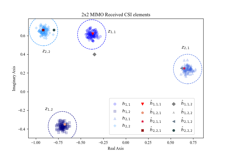
Figure 1: Measured 2x2 MIMO CSI elements with receiver noise

As an example, consider Fig. 1 illustrating the measured CSI elements for the ${2\times 2}$ MIMO case. The markers in shades of blue indicate measured samples gathered during the initial authentication. Comparing the red-shaded CSI elements from $\hat{\textit{h}}_{n,m,1}$ and gray-shaded elements in $\hat{\textit{h}}_{n,m,2}$, the desired outcome is that $\hat{\textit{h}}_{n,m,1}$ will authenticate, but $\hat{\textit{h}}_{n,m,2}$ will not authenticate due to $\hat{\textit{h}}_{1,1,2}$ likely being outside of the error tolerance for $z_{1,1}$, where for this case $z=5\lambda_{ave}^{\frac{1}{2}}$ for all $n$$m$ terms.

Given an ${N\times M}$ array of normally distributed random variables, we can determine the probability of one transmitter being accidentally authenticated as another based on the error tolerance for the first transmitter, z. Let $a_{n,m}$ be the real part and $b_{n,m}$ be the imaginary part of the complex value for the true CSI element, $h_{n,m}=a_{n,m}+jb_{n,m}$. Both $a_{n,m}$ and $b_{n,m}$ are independent Gaussian random variables with variance $\sigma^{2}/2$. To this variable, we add the result of the receiver noise, $\bm{\epsilon}$. The real and imaginary parts of $\epsilon_{n,m}$ are zero-mean independent Gaussian distributed random variables each with sample mean covariance $\Sigma_{\overline{\epsilon}_{n,m}}$.

For a transmitter to be authenticated, $\mathcal{H}_{0}$ must be satisfied for every CSI element, $\textit{h}_{n,m}$. Given $\textit{h}_{n,m}=a_{n,m}+jb_{n,m}$, we can determine the probability that another transmitter will be authenticated. Let $z=5\lambda_{ave}^{\frac{1}{2}}$ where $\lambda_{ave}$ is the average eigenvalue from the receiver noise covariance matrix, $\bm{\Sigma}_{\overline{\epsilon}_{n,m}}$ and $u$ and $v$ be the respective real and imaginary parts of the CSI from another transmitter. The probability of $u+jv$ resulting in $\mathcal{H}_{0}$ for $h_{n,m}$ is

$$\begin{split}P([u+jv]\in\mathcal{D}_{n,m})=\iint_{\mathcal{D}_{n,m}}\frac{\exp{\left(-\frac{u^{2}+v^{2}}{\sigma^{2}}\right)}}{2\pi\sqrt{|\bm{\Sigma}_{u,v}|}}\,du\,dv\\ where,\cr\mathcal{D}_{n,m}=\{(u,v)\mid\left(u-a_{n,m}\right)^{2}+\left(v-b_{n,m}\right)^{2}\leq z^{2}\}\\ \\ \bm{\mu}_{u,v}=\begin{pmatrix}0\\ 0\end{pmatrix},\qquad\bm{\Sigma}_{u,v}=\begin{pmatrix}\sigma^{2}/2&0\\ 0&\sigma^{2}/2\end{pmatrix}\end{split}$$ (4)

With independent $u$ and $v$, (4) can be evaluated using ${P(X\cap Y)=P(Y|X)\cdot P(X)}$, where $P(X)$ is the probability that ${{a_{n,m}-z}\leq\enspace u\enspace\leq{a_{n,m}+z}}$, and $P(Y|X)$ is the probability that ${{b_{n,m}\shortminus\sqrt{z^{2}\shortminus(u\shortminus a_{n,m})^{2}}}\leq v\leq{b_{n,m}+\sqrt{z^{2}\shortminus(u\shortminus a_{n,m})^{2}}}}$. Therefore,

$$\begin{split}\begin{aligned} P([u+jv]&\in\mathcal{D}_{n,m})=\left(Q(A)-Q(B)\right)\cdot\left(Q(C)-Q(D)\right)\\ where,\cr&A=\frac{a_{n,m}-z}{\sigma}\quad B=\frac{a_{n,m}+z}{\sigma}\\ &C=\frac{b_{n,m}-\sqrt{z^{2}-\left(u-a_{n,m}\right)^{2}}}{\sigma}\\ &D=\frac{b_{n,m}+\sqrt{z^{2}-\left(u-a_{n,m}\right)^{2}}}{\sigma}\\ andthe$ Q(\cdot) $functionis\cr&Q(x)=\int_{x}^{+\infty}\frac{1}{\sqrt{2\pi}}\exp\left(-\frac{t^{2}}{2}\right)dt\end{aligned}\end{split}$$ (5)

The transmitter must satisfy $\mathcal{H}_{0}$ for every CSI element. The probability for authentication in a MIMO channel with $M$ transmit antennas and $N$ receive antennas is then

$$\begin{gathered}\prod_{m=1}^{M}\prod_{n=1}^{N}P([u_{n,m}+jv_{n,m}]\in\mathcal{D}_{n,m})\\ \mathcal{D}_{n,m}=\{(u_{n,m},v_{n,m})\mid\left(u_{n,m}-a_{n,m}\right)^{2}\\ \qquad\qquad+\left(v_{n,m}-b_{n,m}\right)^{2}\leq z^{2}\}\\ \end{gathered}$$ (6)

Simulating (5) and (6) with $a_{n,m},b_{n,m},u,$ and $v$ all distributed as $\mathcal{N}(0,0.5)$, Fig. 2 illustrates how unlikely an accidental authentication will be as the number of antenna elements of the receiver and transmitter are increased and the threshold is reduced.

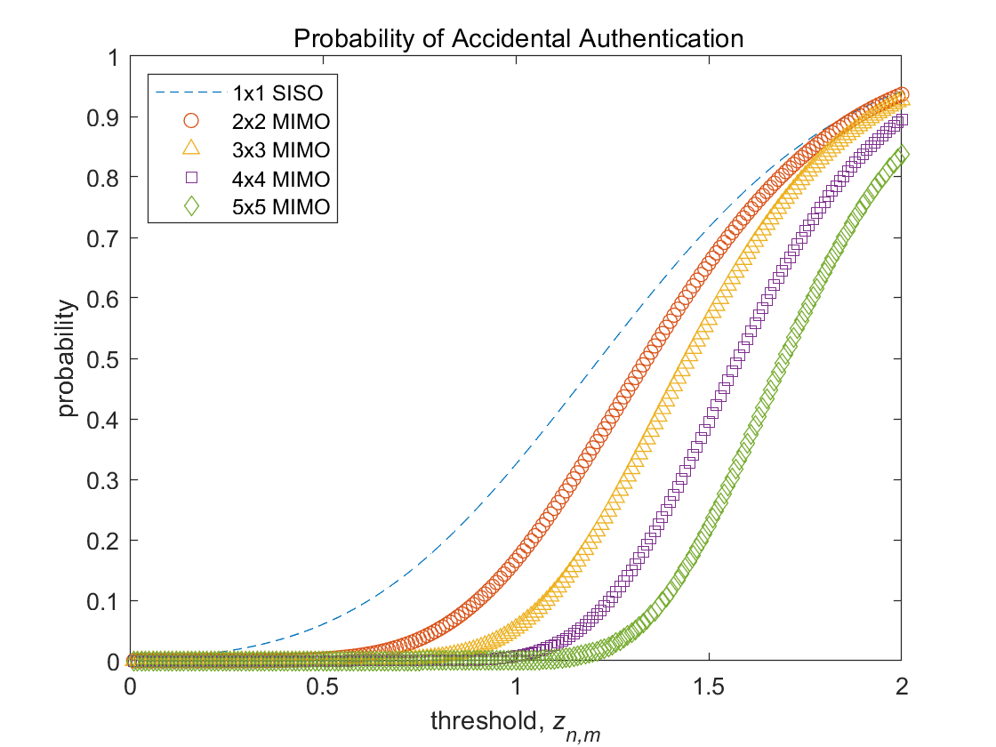
Figure 2: Probability of authentication for various MIMO configurations and thresholds

To implement this authentication scheme and determine which hypothesis $\hat{\textit{h}}_{n,m,k}$ satisfies, we require advance knowledge of the noise power our receiver imparts to H to determine $z$ and that may change over time and be different among devices. Instead, we will allow a neural network to implicitly determine the threshold and perform the authentication decision. We created a GAN that is trained on authentic samples from a dataset and samples produced by a generative model. The discriminative model then learned the characteristics of $\textit{h}_{n,m}$ and $\bm{\Sigma}_{\overline{\epsilon}_{n,m}}$. Following training, two testing datasets validated the performance of the discriminative model to accurately distinguish H between trusted and untrusted transmitters.

IV System Model

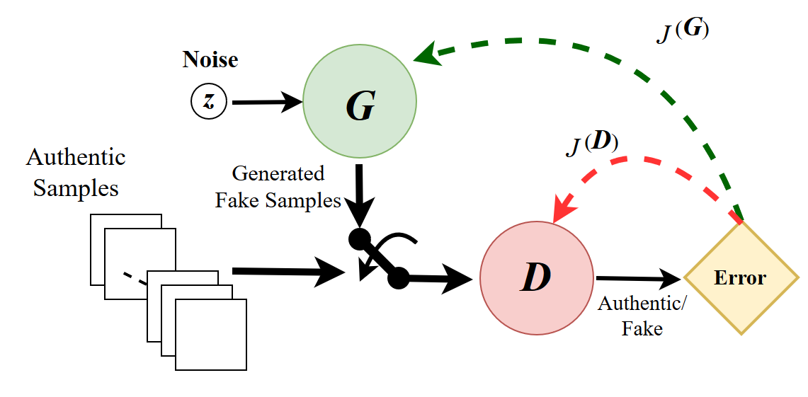
Figure 3: Training a generative adversarial network

We consider a wireless MIMO communications channel with trusted users and untrusted users, some of the latter group who are malicious adversaries. The adversaries have resources available to change their antenna characteristics, transmitter RF path timing, output power, and/or present reflectors between themselves and the receiver. Thus, they are able to change their CSI as measured by the receiver. To defeat this scenario, the discriminative model at the receiver is adversarially trained by a generative model that creates authentic looking CSI samples.

During training, the discriminative model, $\mathcal{D}$, receives authentic samples from the training data or fake samples generated by the generative model, $\mathcal{G}$. The generative model creates fake samples based on a function from random variable input, $\mathit{z}$, and the parameters in $\mathcal{G}$. The discriminative model then assigns a probability from zero to one based on whether the sample is fake (0.0) or authentic (1.0). Fig. 3 shows a functional depiction of a GAN in training, where $\mathit{J^{(D)}}$ and $\mathit{J^{(G)}}$ are the loss functions for the discriminative model and the generative model, respectively.

The adversarial competition in the GAN is a minimax game where the discriminative model attempts to correctly label training samples from a distribution produced by CSI matrix elements, $p_{data}(h_{n,m})$, and fake training samples created by the generator. The discriminative model is trained to maximize the probability of assigning the correct label, while the generative model is trained to minimize the same probability. The value function that describes this relationships from the original work by Goodfellow [22] is given by

$$\begin{split}\min_{G}\max_{D}V(D,G)&=\mathbb{E}_{x\sim p_{data}(x)}[\log D(x)]\\ &\qquad+\mathbb{E}_{z\sim p_{z}(z)}[\log(1-D(G(z)))]\end{split}$$ (7)

where $\mathit{D(x)}$ is the probability that $\mathit{x}$ came from the data distribution $\mathit{p_{data}(x)}$ containing authentic training samples, and $\mathit{D(G(z))}$ is the estimate of the probability that the discriminator incorrectly identifies the fake instance as authentic. The generator network attempts to maximize $\mathit{D(G(z))}$, while the discriminator network tries to minimize it. The generator creates samples, $\mathit{G(z)}$, based on the parameter values in $\mathit{G}$ and the random values $z$ provided to the generator consistent with $\mathit{p_{z}(z)}$.

As each entity adversarially trains each other, they learn to improve their individual performance. When the discriminative model correctly identifies fake samples created by the generative model, the generative network will update its parameter weights through backpropagation to make more realistic samples. Likewise, the discriminative model will update its parameter weights when it incorrectly identifies real or fake samples. The results of this training are a generator neural network adept at creating data that closely mimics training data and a discriminator neural network that can identify all but the best fakes.

V Simulation

The GAN processed a single subcarrier in a MIMO ${4\times 4}$ configuration. Therefore, the discriminative model has 16 complex inputs and 1 real output, while the generative model has 1 real input and 16 complex outputs. The inputs for the discriminative model and the outputs for the generative model represent the complex elements in the CSI matrix.

V-A GAN development

TABLE I: GAN architecture

Discriminator:
	Layer	output size	activation
	Input 1: $x\sim p_{data}(x_{1,1})$	2
	Input 2: $x\sim p_{data}(x_{1,2})$	2
	⋮	⋮
	Input 16: $x\sim p_{data}(x_{4,4})$	2
	Concatenated	32
	Fully connected	64	LeakyReLU (alpha = 0.3)
	Dropout = 0.2
	Fully connected	32	LeakyReLU (alpha = 0.3)
	Dropout = 0.2
	Output	1	Sigmoid
Generator:
	Layer	output size	activation
	Input: $z\sim p_{z}(z)$	5
	Fully connected	16	LeakyReLU (alpha = 0.3)
	Fully connected	32	LeakyReLU (alpha = 0.3)
	Fully connected	64	tanh
	Output 1	2	linear
	Output 2	2	linear
	⋮	⋮	⋮
	Output 16	2	linear

The GAN is implemented using the Python programming language, Keras [30] front-end, and Tensorflow [31] back-end. Additionally, Numpy, Pandas, and Matplotlib Python libraries were used. The overall GAN design is summarized in Table I, with a total of 19,425 parameters. The file size of the discriminator network was 104 KB.

The discriminator network, $\mathcal{D}$, has 16 inputs of size 2 merged into one concatenated layer. Each input has 2 nodes to accommodate the real and imaginary parts of the complex CSI matrix element. Two additional fully connected layers of size 64 and 32 with LeakyReLU activations (alpha = 0.3) follow. Both of these hidden layers use Dropout of 0.2 to prevent overfitting. The output layer of size 1 is fully connected and uses a sigmoid activation to provide values [0.0, 1.0]. The learning rate for $\mathcal{D}$ was 0.0003 using the Adam [32] optimizer.

The generator network, $\mathcal{G}$, has a single input with 5 nodes fully connected to the first hidden layer of size 16. Two additional hidden layers of sizes 32 and 64 are again fully connected using LeakyReLU (alpha = 0.3) and tanh activations respectively. Finally, 16 output layers of size 2 are connected using linear activations. The learning rate for $\mathcal{G}$ was 0.0009 using the Adam optimizer.

V-B Datasets

A master dataset was created by adding measurement error in the form of AWGN across a range of signal to noise ratio (SNR) levels to a single ${4\times 4}$ CSI matrix composed of 16 circularly symmetric Gaussian complex values with zero mean, and unit variance, $\mathcal{CN}(0,1)$. The SNR values ranged from 0 dB to 30 dB in steps of 2 dB, and 1,000 samples were created at each SNR level. Each sample is a ${4\times 4}$ complex matrix.

Splitting evenly across SNR levels, the training dataset uses 70% of the master dataset samples, reserving 30% for the testing dataset. Two testing datasets were created, each consisting of 700 samples for each SNR value. In addition to the valid samples taken from the master dataset, 400 more testing samples were created to simulate two different operating scenarios.

The first testing dataset replicated the accidental authentication case. There are six transmitters, one of which should be authenticated. The 300 samples taken from the master dataset represent the transmitter that should be authenticated. For the remaining transmitters, five new ${4\times 4}$ CSI matrices with elements taken from $\mathcal{CN}(0,1)$ were created. To each matrix, AWGN at varying SNR values was added to produce 80 samples at each SNR value. These samples were then added to the accidental authentication dataset, resulting in 300 legitimate samples and 400 illegitimate samples. We will refer to this dataset as the accidental authentication test dataset.

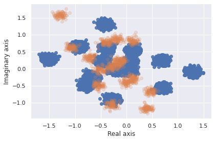
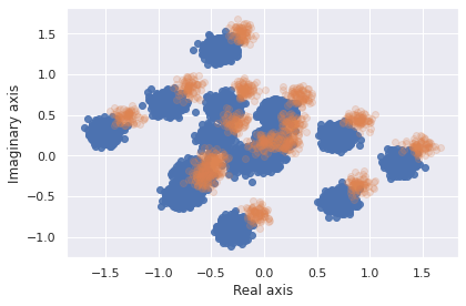
(a)                                       (b)

Figure 4: Samples from the (a) accidental authentication and (b) nefarious users test datasets at 20 dB.

The second testing dataset emulated five nefarious users attempting to authenticate by matching the CSI matrix of a single legitimate transmitter. If by some unlikely method, an adversary were able to know the channel characteristics between two legitimately authenticated transmitters, such as described by Shi et al. in [33], the adversary may also have the resources necessary to spoof their transmitted CSI to appear as another transmitter’s received CSI. As before, 300 samples from the master dataset for each of the 16 SNR levels ranging from 0 dB to 30 dB in steps of 2 dB are the legitimate samples. To complete this dataset, five different complex number offsets were added to the original legitimate CSI matrix. Samples were created as previously described by the addition of AWGN again resulting in 300 legitimate samples and 400 illegitimate samples. We will refer to this dataset as the nefarious users test dataset.

Samples from each dataset are shown in Fig. 4, where blue dots correspond to the 16 clusters of legitimate samples, and the orange circles represent illegitimate samples that should not be authenticated. Note that only one example from the illegitimate test group is shown for each dataset. Training was restricted to a maximum of 50 epochs in mini-batches of 64 samples.

V-C Results

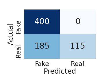
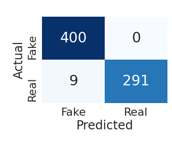
(a) SNR = 0 dB                   (b) SNR = 4 dB

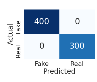
(c) SNR = 8 dB                   (d) SNR = 10 dB

Figure 5: GAN discriminator performance against accidental authentication test dataset with SNR levels at (a) 0 dB, (b) 4 dB, (c) 8 dB, (d) 12 dB.

The performance of the discriminative model indicates the viability of using a GAN for physical-layer authentication using CSI. To illustrate the performance, we use confusion matrices to show how the discriminator assigns samples from the test datasets. The horizontal axis is the predicted result from the discriminator on whether or not authentication should be granted. If the discriminator assesses the sample to be legitimate, the sample is tallied in the “Real” column. If the discriminator’s result predict that the sample is illegitimate and should not be authenticated, the sample is allocated to the “Fake” column. The vertical axis is the ground truth of the sample from the dataset, where legitimate samples are assigned to the “Real” row, and illegitimate samples are shown in the “Fake” row.

Against the accidental authentication testing dataset, the discriminator achieves 100% accuracy for SNR greater than or equal to 10 dB. As shown in Fig. 5, for SNR less than 10 dB, the discriminator makes errors in correctly identifying legitimate samples but never allows illegitimate samples to be authenticated.

For the nefarious user testing dataset, the discriminator doesn’t achieve 100% until the SNR reaches 20 dB. As shown in Fig. 6, in addition to mischaracterizing legitimate samples, the discriminator allows some number of illegitimate samples to be authenticated, since there are samples counted in the “Fake” row and “Real” column.

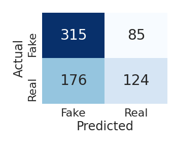
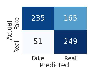
(a) SNR = 0 dB                   (b) SNR = 4 dB

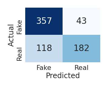
(c) SNR = 8 dB                   (d) SNR = 20 dB

Figure 6: GAN discriminator performance against nefarious users test dataset with SNR levels at (a) 0 dB, (b) 4 dB, (c) 8 dB, (d) 20 dB.

In order to compare the GAN-trained discriminator’s performance, we apply the same datasets to the hypothesis test in (3), and to three machine learning algorithms. Because the master dataset does not contain illegitimate samples, the techniques we use are limited to one-class, novelty, or anomaly detection algorithms. We employ LOF, iForest, and OC-SVM. These techniques are available and were implemented from the Scikit-learn project [21].

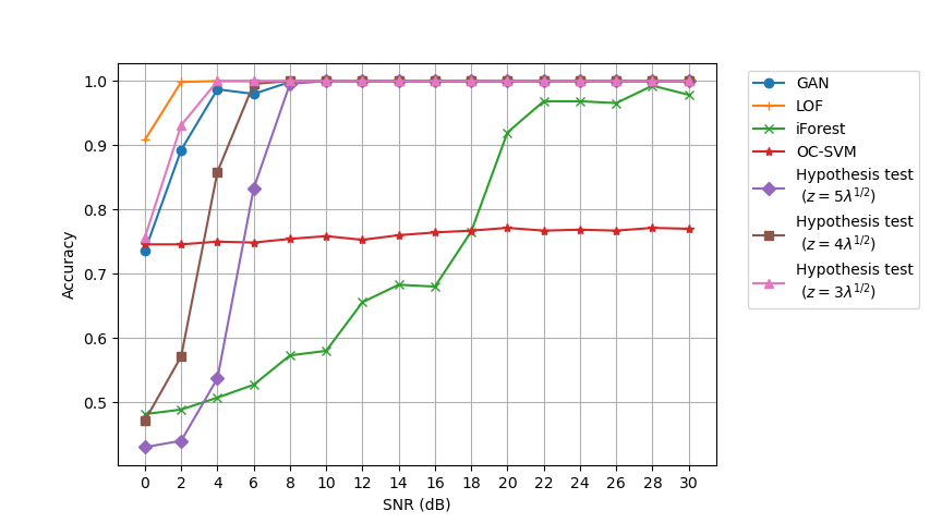
Figure 7: Accuracy vs SNR for accidental authentication dataset

For the accidental authentication test dataset, Fig. 7 shows the accuracy performance for the machine learning techniques. We see that the LOF algorithm is superior for all SNR levels and that the GAN and hypothesis test with ${z=3\lambda^{\frac{1}{2}}}$ are very close in performance.

Fig. 8 illustrates the accuracy of the machine learning techniques against the nefarious users test dataset. While LOF is the first algorithm to reach 100% accuracy, its performance at low SNR values against this dataset is outmatched by the GAN. We noted that all techniques including the GAN, as we’ve seen in Fig. 6, incorrectly categorize illegitimate samples as “Real” for low SNR against the nefarious users who are able to closely match the CSI of legitimate transmitters.

Adjustment of hyperparameters and training methodology for the GAN can be applied to improve results. For example, by increasing the mini-batch size, we saw an improvement in identifing the illegitimate samples. Unfortunately, this also caused a reduction in the number of legitimate samples identified. Changes to the original GAN architecture in this work is left for future refinement.

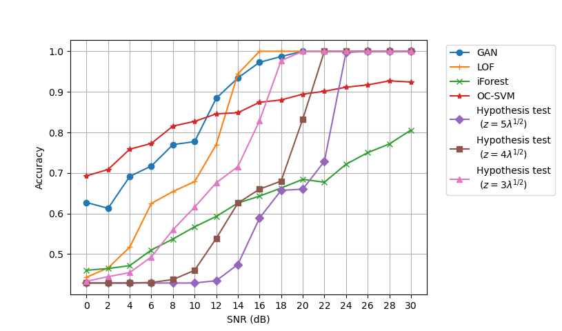
Figure 8: Accuracy performance vs SNR for nefarious users dataset

VI Conclusion and Future Work

We showed how CSI could be used as a method to provide physical-layer authentication. Our analysis illustrated that the probability of accidentally authenticating other transmitters decreases as the number of receive and transmit antennas are increased and a threshold value is judiciously applied. We then developed a GAN trained on a dataset of CSI matrices to perform physical-layer authentication in an adversarial environment. After training less than 50 epochs, the discriminator reached 100% accuracy on two seperate testing datasets, implicitly determining appropriate thresholds for received CSI matrix elements. Across all levels of AWGN, the LOF algorithm was best at reaching 100% accuracy.

This paper demonstrated how physical-layer authentication can be accomplished in a flat fading single subchannel environment. By applying this concept to multiple subchannels, there is an opportunity for obtaining robust multi-channel characteristics that can be used to identify a transmitter for authentication. Furthermore, the hyperparameters of the GAN should be optimized and reevaluated on additional training and test datasets to demonstrate effectiveness in a variety of wireless environments.

References

- [1] A. Géron, Hands-on machine learning with Scikit-Learn and TensorFlow : concepts, tools, and techniques to build intelligent systems, first edition ed. Sebastopol, CA: O’Reilly Media, 2017. [Online]. Available: http://shop.oreilly.com/product/0636920052289.do
- [2] V. Brik, S. Banerjee, M. Gruteser, and S. Oh, “Wireless device identification with radiometric signatures,” in Proceedings of the 14th ACM international conference on Mobile computing and networking - MobiCom ’08. San Francisco, California, USA: ACM Press, 2008, p. 116.
- [3] O. Gungor and C. E. Koksal, “On the Basic Limits of RF-Fingerprint-Based Authentication,” IEEE Transactions on Information Theory, vol. 62, no. 8, pp. 4523–4543, Aug. 2016.
- [4] A. C. Polak, S. Dolatshahi, and D. L. Goeckel, “Identifying Wireless Users via Transmitter Imperfections,” IEEE Journal on Selected Areas in Communications, vol. 29, no. 7, pp. 1469–1479, Aug. 2011.
- [5] J. K. Tugnait, “Wireless User Authentication via Comparison of Power Spectral Densities,” IEEE Journal on Selected Areas in Communications, vol. 31, no. 9, pp. 1791–1802, Sep. 2013.
- [6] Yingbin Liang, H. Poor, and S. Shamai, “Secure Communication Over Fading Channels,” IEEE Transactions on Information Theory, vol. 54, no. 6, pp. 2470–2492, Jun. 2008.
- [7] N. Al Khanbashi, N. Al Sindi, S. Al-Araji, N. Ali, Z. Chaloupka, V. Yenamandra, and J. Aweya, “Real time evaluation of RF fingerprints in wireless LAN localization systems,” in 2013 10th Workshop on Positioning, Navigation and Communication (WPNC), Mar. 2013, pp. 1–6.
- [8] L. Xiao, L. Greenstein, N. Mandayam, and W. Trappe, “A Physical-Layer Technique to Enhance Authentication for Mobile Terminals,” in 2008 IEEE International Conference on Communications, May 2008, pp. 1520–1524, iSSN: 1550-3607, 1938-1883.
- [9] K. Yu and B. Ottersten, “Models for MIMO propagation channels: a review,” Wireless Communications and Mobile Computing, vol. 2, no. 7, pp. 653–666, 2002. [Online]. Available: https://onlinelibrary.wiley.com/doi/abs/10.1002/wcm.78
- [10] W. C. Jakes, Ed., Microwave mobile communications, nachdr. ed., ser. An IEEE Press classic reissue. New York, NY: IEEE Press [u.a.], 1995, oCLC: 249569885.
- [11] H. Liu, Y. Wang, J. Liu, J. Yang, Y. Chen, and H. V. Poor, “Authenticating Users Through Fine-Grained Channel Information,” IEEE Transactions on Mobile Computing, vol. 17, no. 2, pp. 251–264, Feb. 2018, conference Name: IEEE Transactions on Mobile Computing.
- [12] R. Liao, H. Wen, F. Pan, H. Song, A. Xu, and Y. Jiang, “A Novel Physical Layer Authentication Method with Convolutional Neural Network,” in 2019 IEEE International Conference on Artificial Intelligence and Computer Applications (ICAICA), Mar. 2019, pp. 231–235, iSSN: null.
- [13] Q. Wang, H. Li, D. Zhao, Z. Chen, S. Ye, and J. Cai, “Deep Neural Networks for CSI-Based Authentication,” IEEE Access, vol. 7, pp. 123 026–123 034, 2019, conference Name: IEEE Access.
- [14] R.-F. Liao, H. Wen, J. Wu, F. Pan, A. Xu, Y. Jiang, F. Xie, and M. Cao, “Deep-Learning-Based Physical Layer Authentication for Industrial Wireless Sensor Networks,” Sensors (Basel, Switzerland), vol. 19, no. 11, May 2019. [Online]. Available: https://www.ncbi.nlm.nih.gov/pmc/articles/PMC6603790/
- [15] R. Liao, H. Wen, J. Wu, F. Pan, A. Xu, H. Song, F. Xie, Y. Jiang, and M. Cao, “Security Enhancement for Mobile Edge Computing Through Physical Layer Authentication,” IEEE Access, vol. 7, pp. 116 390–116 401, 2019.
- [16] A. Y. Abyaneh, A. H. G. Foumani, and V. Pourahmadi, “Deep Neural Networks Meet CSI-Based Authentication,” arXiv:1812.04715 [cs, eess, stat], Nov. 2018, arXiv: 1812.04715. [Online]. Available: http://arxiv.org/abs/1812.04715
- [17] M. M. Breunig, H.-P. Kriegel, R. T. Ng, and J. Sander, “LOF: identifying density-based local outliers,” ACM SIGMOD Record, vol. 29, no. 2, pp. 93–104, May 2000. [Online]. Available: http://doi.org/10.1145/335191.335388
- [18] F. T. Liu, K. M. Ting, and Z.-H. Zhou, “Isolation Forest,” in 2008 Eighth IEEE International Conference on Data Mining, Dec. 2008, pp. 413–422, iSSN: 2374-8486.
- [19] ——, “Isolation-Based Anomaly Detection,” ACM Transactions on Knowledge Discovery from Data, vol. 6, no. 1, pp. 3:1–3:39, Mar. 2012. [Online]. Available: http://doi.org/10.1145/2133360.2133363
- [20] B. Schölkopf, J. C. Platt, J. Shawe-Taylor, A. J. Smola, and R. C. Williamson, “Estimating the Support of a High-Dimensional Distribution,” Neural Computation, vol. 13, no. 7, pp. 1443–1471, Jul. 2001. [Online]. Available: https://www.mitpressjournals.org/doi/abs/10.1162/089976601750264965
- [21] F. Pedregosa, G. Varoquaux, A. Gramfort, V. Michel, B. Thirion, O. Grisel, M. Blondel, P. Prettenhofer, R. Weiss, V. Dubourg, J. Vanderplas, A. Passos, D. Cournapeau, M. Brucher, M. Perrot, and . Duchesnay, “Scikit-learn: Machine Learning in Python,” Journal of Machine Learning Research, vol. 12, no. 85, pp. 2825–2830, 2011. [Online]. Available: http://jmlr.org/papers/v12/pedregosa11a.html
- [22] I. J. Goodfellow, J. Pouget-Abadie, M. Mirza, B. Xu, D. Warde-Farley, S. Ozair, A. Courville, and Y. Bengio, “Generative Adversarial Nets,” in Proceedings of the 27th International Conference on Neural Information Processing Systems - Volume 2, ser. NIPS’14. Cambridge, MA, USA: MIT Press, 2014, pp. 2672–2680, event-place: Montreal, Canada. [Online]. Available: http://dl.acm.org/citation.cfm?id=2969033.2969125
- [23] C. Ledig, L. Theis, F. Huszár, J. Caballero, A. Cunningham, A. Acosta, A. Aitken, A. Tejani, J. Totz, Z. Wang, and W. Shi, “Photo-Realistic Single Image Super-Resolution Using a Generative Adversarial Network,” in 2017 IEEE Conference on Computer Vision and Pattern Recognition (CVPR), Jul. 2017, pp. 105–114, iSSN: 1063-6919.
- [24] K. Armanious, C. Jiang, M. Fischer, T. Küstner, T. Hepp, K. Nikolaou, S. Gatidis, and B. Yang, “MedGAN: Medical Image Translation using GANs,” Computerized Medical Imaging and Graphics, p. 101684, Nov. 2019. [Online]. Available: http://www.sciencedirect.com/science/article/pii/S0895611119300990
- [25] J. Bao, D. Chen, F. Wen, H. Li, and G. Hua, “CVAE-GAN: Fine-Grained Image Generation through Asymmetric Training,” in 2017 IEEE International Conference on Computer Vision (ICCV), Oct. 2017, pp. 2764–2773, iSSN: 2380-7504.
- [26] T. J. O’Shea, T. Roy, N. West, and B. C. Hilburn, “Physical Layer Communications System Design Over-the-Air Using Adversarial Networks,” in 2018 26th European Signal Processing Conference (EUSIPCO), Sep. 2018, pp. 529–532.
- [27] D. Roy, T. Mukherjee, M. Chatterjee, E. Blasch, and E. Pasiliao, “RFAL: Adversarial Learning for RF Transmitter Identification and Classification,” IEEE Transactions on Cognitive Communications and Networking, pp. 1–1, 2019.
- [28] Q. Li, H. Qu, Z. Liu, N. Zhou, W. Sun, S. Sigg, and J. Li, “AF-DCGAN: Amplitude Feature Deep Convolutional GAN for Fingerprint Construction in Indoor Localization Systems,” IEEE Transactions on Emerging Topics in Computational Intelligence, pp. 1–13, 2019.
- [29] L. Xiao, L. J. Greenstein, N. B. Mandayam, and W. Trappe, “Using the physical layer for wireless authentication in time-variant channels,” IEEE Transactions on Wireless Communications, vol. 7, no. 7, pp. 2571–2579, Jul. 2008.
- [30] F. Chollet, et al., Keras, 2015. [Online]. Available: https://keras.io
- [31] M. Abadi, et al., “TensorFlow: Large-Scale Machine Learning on Heterogeneous Systems,” 2015. [Online]. Available: https://www.tensorflow.org/
- [32] D. P. Kingma and J. Ba, “Adam: A Method for Stochastic Optimization,” arXiv:1412.6980 [cs], Jan. 2017, arXiv: 1412.6980. [Online]. Available: http://arxiv.org/abs/1412.6980
- [33] Y. Shi, K. Davaslioglu, and Y. E. Sagduyu, “Generative Adversarial Network for Wireless Signal Spoofing,” in Proceedings of the ACM Workshop on Wireless Security and Machine Learning - WiseML 2019. Miami, FL, USA: ACM Press, 2019, pp. 55–60. [Online]. Available: http://dl.acm.org/citation.cfm?doid=3324921.3329695