DINO: Distributed Newton-Type Optimization Method

Abstract

We present a novel communication-efficient Newton-type algorithm for finite-sum optimization over a distributed computing environment. Our method, named DINO, overcomes both theoretical and practical shortcomings of similar existing methods. Under minimal assumptions, we guarantee global sub-linear convergence of DINO to a first-order stationary point for general non-convex functions and arbitrary data distribution over the network. Furthermore, for functions satisfying Polyak-Lojasiewicz (PL) inequality, we show that DINO enjoys a linear convergence rate. Our proposed algorithm is practically parameter free, in that it will converge regardless of the selected hyper-parameters, which are easy to tune. Additionally, its sub-problems are simple linear least-squares, for which efficient solvers exist. Numerical simulations demonstrate the efficiency of DINO as compared with similar alternatives.

1 Introduction

Consider the generic finite-sum optimization problem

$$\min_{{\bf w}\in\mathbb{R}^{d}}\bigg{\{}f({\bf w})\triangleq\frac{1}{m}\sum_{i=1}^{m}f_{i}({\bf w})\bigg{\}},$$ (1)

in a centralized distributed computing environment comprised of one central driver machine communicating to $m$ worker machines, where each worker $i$ only has access to $f_{i}$. A common application of this problem is where each worker $i$ has access to a portion of $n$ data points $\{{\bf x}_{1},\ldots,{\bf x}_{n}\}$, indexed by a set $S_{i}\subseteq\{1,\ldots,n\}$, with

$$f_{i}({\bf w})=\frac{|S_{i}|}{n}\sum_{j\in S_{i}}\ell_{j}({\bf w};{\bf x}_{j}),$$ (2)

where $\ell_{i}$ is a loss function corresponding to ${\bf x}_{i}$ and parameterized by ${\bf w}$. For example, such settings are popular in industry in the form of federated learning when data is collected and processed locally, which increases computing resources and facilitates data privacy [1]. Another example is in big data regimes, where it is more practical, or even necessary, to partition and store large datasets on separate machines [2]. Distributing machine learning model parameters is also becoming a necessity as some highly successful models now contain billions of parameters, such as GPT-2 [3, 4].

The need for distributed computing has motivated the development of many frameworks. For example, the popular machine learning packages PyTorch [5] and Tensorflow [6] contain comprehensive functionality for distributed training of machine learning models. Despite many benefits to distributed computing, there are significant computational bottlenecks, such as those introduced through bandwidth and latency [7, 8, 9]. Frequent transmission of data is expensive in terms of time and physical resources [2]. For example, even transferring data on a local machine can be the main contributor to energy consumption [10].

With the bottleneck of communication, there has recently been significant focus on developing communication-efficient distributed optimization algorithms. This is particularly apparent in regards to popular first-order methods, such as stochastic gradient descent (SGD) [11, 12, 13, 14, 15, 16]. As first-order methods solely rely on gradient information, which can often be computed easily in parallel, they are usually straightforward to implement in a distributed setting. However, their typical inherent nature of performing many computationally inexpensive iterations, which is suitable and desirable on a single machine, leads to significant data transmission costs and ineffective utilization of increased computing resources in a distributed computing environment [17].

Related Work

In contrast to first-order methods, second-order methods perform more computation per iteration and, as a result, often require far fewer iterations to achieve similar results. In distributed settings, these properties directly translate to more efficient utilization of the increased computing resources and far fewer communications over the network. Motivated by this potential, several distributed Newton-type algorithms have recently been developed, most notably DANE [18], DiSCO [2], InexactDANE and AIDE [19], GIANT [17], and DINGO [20].

While each of these second-order distributed methods have notable benefits, they all come with disadvantages that limit their applicability. DiSCO and GIANT are simple to implement, as they involve sub-problems in the form of linear systems. Whereas, the sub-problems of InexactDANE and AIDE involve non-linear optimization problems and their hyper-parameters are difficult and time consuming to tune. DiSCO and GIANT rely on strong-convexity assumptions, and GIANT theoretically requires particular function form and data distribution over the network in (2). In contrast, InexactDANE and AIDE are applicable to non-convex objectives. DINGO’s motivation is to not require strong-convexity assumptions, i.e., it converges for invex problems [21], and still be easy to use in practice, i.e., simple to tune hyper-parameters and linear-least squares sub-problems. DINGO achieves this by optimizing the norm of the gradient as a surrogate function. Thus, it may converge to a local maximum or saddle point in non-invex problems. Moreover, the theoretical analysis of DINGO is limited to exact update.

Table 1: Comparison of problem class, function form and data distribution. DINGO is suited to invex problems in practice, as it may converge to a local maximum or saddle point in non-invex problems [20]. This is a modified table from [20].

	Problem Class	Function Form	Data Distribution
DINO	Non-Convex	Any	Any
DINGO [20]	Invex	Any	Any
GIANT [17]	Strongly Convex	$\ell_{j}({\bf w};{\bf x}_{j})=\psi_{j}(\langle{\bf w},{\bf x}_{j}\rangle)+\gamma\|{\bf w}\|^{2}$ in (2)	$|S_{i}|>d$ in (2)
DiSCO [2]	Strongly Convex	Any	Any
InexactDANE [19]	Non-Convex	Any	Any
AIDE [19]	Non-Convex	Any	Any

Table 2: Comparison of number of hyper-parameters (under exact update) and communication rounds per iteration (under inexact update). Additional hyper-parameters may be introduced under inexact update, such as in the solver used for the non-linear optimization sub-problems of InexactDANE and AIDE. We assume DINO, DINGO and GIANT use two communication rounds per iteration for line-search. This is a modified table from [20].

	Number of Hyper-parameters	Communication Rounds Per
	(Under Exact Update)	Iteration (Under Inexact Update)
DINO	$2$	$6$
DINGO [20]	$2$	$4$ to $8$
GIANT [17]	$0$	$6$
DiSCO [2]	$0$	$2+2\cdot(\text{sub-problem iterations})$
InexactDANE [19]	$2$	$4$
AIDE [19]	$3$	$4\cdot(\text{inner InexactDANE iterations})$

Contributions

We present a novel communication-efficient distributed second-order optimization algorithm that combines many of the above-mentioned desirable properties. Our algorithm is named DINO, for “DIstributed Newton-type Optimization method”. Our method is inspired by the novel approach of DINGO, which allowed it to circumvent various theoretical and practical issues of other methods. However, unlike DINGO, we minimize (1) directly and our analysis involves less assumptions and is under inexact update; see Tables 1 and 2 for high-level algorithm properties.

A summary of our contributions is as follows.

1. The analysis of DINO is simple, intuitive, requires very minimal assumptions and can be applied to arbitrary non-convex functions. Namely, by requiring only Lipschitz continuous gradients $\mathbf{\nabla}f_{i}$, we show global sub-linear convergence for general non-convex (1). Recall that additional assumptions are typically required for the analysis of second-order methods. Such common assumptions include strong convexity, e.g., in [22], and Lipschitz continuous Hessian, e.g., in [23], which are both required for GIANT. Although the theory of DINGO does not require these, it still assumes additional unconventional properties of the Hessian and, in addition, is restricted to invex problems, as a strict sub-class of general non-convex models. Furthermore, in our analysis, we don’t assume specific function form or data distribution for applications of the form (2). For example, this is in contrast to GIANT, which is restricted to loss functions involving linear predictor models and specific data distributions.

2. DINO is practically parameter free, in that it will converge regardless of the selected hyper-parameters. This is in sharp contrast to many first-order methods. The hyper-parameters of InexactDANE and AIDE require meticulous fine-tuning and these are sensitive to the given application. DINO is simple to tune and performs well across a variety of problems without modification of the hyper-parameters.

3. The sub-problems of DINO are simple. Like DINGO, the sub-problems of our method are simple linear least-squares problems for which efficient and robust direct and iterative solvers exists. In contrast, non-linear optimization sub-problems, such as those arising in InexactDANE and AIDE, can be difficult to solve and often involve additional hard to tune hyper-parameters.

Notation and Definitions

Throughout the paper, vectors and matrices are denoted by bold lower-case and bold upper-case letters, respectively, e.g., ${\bf v}$ and ${\mathbf{V}}$. We use regular lower-case and upper-case letters to denote scalar constants, e.g., $d$ or $L$. The common Euclidean inner product is denoted by $\langle{\bf x},{\bf y}\rangle={\bf x}^{T}{\bf y}$ for ${\bf x},{\bf y}\in\mathbb{R}^{d}$. Given a vector ${\bf v}$ and matrix ${\mathbf{A}}$, we denote their vector $\ell_{2}$ norm and matrix spectral norm as $\|{\bf v}\|$ and $\|{\mathbf{A}}\|$, respectively. The Moore–Penrose inverse of ${\mathbf{A}}$ is denoted by ${\mathbf{A}}^{\dagger}$. We let ${\bf w}_{t}\in\mathbb{R}^{d}$ denote the point at iteration $t$. For notational convenience, we denote ${\bf g}_{t,i}\triangleq\mathbf{\nabla}f_{i}({\bf w}_{t})$, ${\bf g}_{t}\triangleq\mathbf{\nabla}f({\bf w}_{t})$, ${\mathbf{H}}_{t,i}\triangleq\mathbf{\nabla}^{2}f_{i}({\bf w}_{t})$ and ${\mathbf{H}}_{t}\triangleq\mathbf{\nabla}^{2}f({\bf w}_{t})$. We also let

$$\tilde{{\mathbf{H}}}_{t,i}\triangleq\begin{bmatrix}{\mathbf{H}}_{t,i}\\ \phi\mathbf{I}\end{bmatrix}\in\mathbb{R}^{2d\times d}\quad\text{and}\quad\tilde{{\bf g}}_{t}\triangleq\begin{pmatrix}{\bf g}_{t}\\ {\bf 0}\end{pmatrix}\in\mathbb{R}^{2d},$$ (3)

where $\phi>0$, $\mathbf{I}$ is the identity matrix, and ${\bf 0}$ is the zero vector. We say that a communication round is performed when the driver uses a broadcast or reduce operation to send or receive information to or from the workers in parallel, respectively. For example, computing the gradient ${\bf g}_{t}$ requires two communication rounds, i.e., the driver broadcasts ${\bf w}_{t}$ and then, using a reduce operation, receives ${\bf g}_{t,i}$ from all workers to then form ${\bf g}_{t}=\sum_{i=1}^{m}{\bf g}_{t,i}/m$.

2 Derivation

In this section, we describe the derivation of DINO, as depicted in Algorithm 1. Each iteration $t$ involves computing an update direction ${\bf p}_{t}$ and a step-size $\alpha_{t}$ and then forming the next iterate ${\bf w}_{t+1}={\bf w}_{t}+\alpha_{t}{\bf p}_{t}$.

Update Direction

When forming the update direction ${\bf p}_{t}$, computing $\tilde{{\mathbf{H}}}_{t,i}^{\dagger}\tilde{{\bf g}}_{t}$ and $(\tilde{{\mathbf{H}}}_{t,i}^{T}\tilde{{\mathbf{H}}}_{t,i})^{-1}{\bf g}_{t}$ constitute the sub-problems of DINO, where $\tilde{{\mathbf{H}}}_{t,i}$ and $\tilde{{\bf g}}_{t}$ are as in (3). Despite these being the solutions of simple linear least-squares problems, it is still unreasonable to assume these will be computed exactly. In this light, we only require that the approximate solutions satisfy the following conditions.

Condition 1 (Inexactness Condition).

For all iterations $t$, all worker machines $i=1,\ldots,m$ are able to compute approximations ${\bf v}_{t,i}^{(1)}$ and ${\bf v}_{t,i}^{(2)}$ of $\tilde{{\mathbf{H}}}_{t,i}^{\dagger}\tilde{{\bf g}}_{t}$ and $(\tilde{{\mathbf{H}}}_{t,i}^{T}\tilde{{\mathbf{H}}}_{t,i})^{-1}{\bf g}_{t}$, respectively, that satisfy:

$$\|\tilde{{\mathbf{H}}}_{t,i}^{T}\tilde{{\mathbf{H}}}_{t,i}{\bf v}_{t,i}^{(1)}-{\mathbf{H}}_{t,i}{\bf g}_{t}\| \leq\varepsilon_{i}^{(1)}\|{\mathbf{H}}_{t,i}{\bf g}_{t}\|,$$ (4a)

$$\|\tilde{{\mathbf{H}}}_{t,i}^{T}\tilde{{\mathbf{H}}}_{t,i}{\bf v}_{t,i}^{(2)}-{\bf g}_{t}\| \leq\varepsilon_{i}^{(2)}\|{\bf g}_{t}\|,$$ (4b)

$$\langle{\bf v}_{t,i}^{(2)},{\bf g}_{t}\rangle >0,$$ (4c)

where $0\leq\varepsilon_{i}^{(1)},\varepsilon_{i}^{(2)}<1$ are constants.

For practical implementations of DINO, as with DINGO, DiSCO and GIANT, we don’t need to compute or store explicitly formed Hessian matrices, i.e., our implementations are Hessian-free. Namely, approximations of $\tilde{{\mathbf{H}}}_{t,i}^{\dagger}\tilde{{\bf g}}_{t}$ and $(\tilde{{\mathbf{H}}}_{t,i}^{T}\tilde{{\mathbf{H}}}_{t,i})^{-1}{\bf g}_{t}$ can be efficiently computed using iterative least-squares solvers that only require access to Hessian-vector products, such as in our implementation described in Section 4. These products can be computed at a similar cost to computing the gradient [24]. Hence, DINO is applicable to (1) with a large dimension $d$.

Condition 1 has a significant practical benefit. Namely, the criteria (4) are practically verifiable as they don’t involve any unknowable terms. Requiring $\varepsilon_{i}^{(1)},\varepsilon_{i}^{(2)}<1$ ensures that the approximations are simply better than the zero vector. The condition in (4c) is always guaranteed if one uses the conjugate gradient method (CG) [25], regardless of the number of CG iterations.

We now derive the update direction ${\bf p}_{t}$ for iteration $t$. Our approach is to construct ${\bf p}_{t}$ so that it is a suitable descent direction of (1). Namely, it satisfies $\langle{\bf p}_{t},{\bf g}_{t}\rangle\leq-\theta\|{\bf g}_{t}\|^{2}$, where $\theta$ is a selected hyper-parameter of DINO. We begin by distributively computing the gradient, ${\bf g}_{t}$, of (1) and then broadcast it to all workers. Each worker $i$ computes the vector ${\bf v}_{t,i}^{(1)}$, as in (4a), lets ${\bf p}_{t,i}=-{\bf v}_{t,i}^{(1)}$ and checks the condition $\langle{\bf v}_{t,i}^{(1)},{\bf g}_{t}\rangle\geq\theta\|{\bf g}_{t}\|^{2}$.

All workers $i$ in

$$\mathcal{I}_{t}\triangleq\big{\{}i=1,\ldots,m\mid\langle{\bf v}_{t,i}^{(1)},{\bf g}_{t}\rangle<\theta\|{\bf g}_{t}\|^{2}\big{\}},$$ (5)

has a local update direction ${\bf p}_{t,i}$ that is not a suitable descent direction of (1), as $\langle{\bf p}_{t,i},{\bf g}_{t}\rangle>-\theta\|{\bf g}_{t}\|^{2}$. We now enforce descent in their local update direction. For this, we consider the problem

$$\min_{{\bf p}_{t,i}} \quad\|{\mathbf{H}}_{t,i}{\bf p}_{t,i}+{\bf g}_{t}\|^{2}+\phi^{2}\|{\bf p}_{t,i}\|^{2}$$ (6)

s.t. $$\hskip 28.45274pt\langle{\bf p}_{t,i},{\bf g}_{t}\rangle\leq-\theta\|{\bf g}_{t}\|^{2},$$

where $\phi$ is a selected hyper-parameter of DINO as in (3). It is easy to see that, when $\langle\tilde{{\mathbf{H}}}_{t,i}^{\dagger}\tilde{{\bf g}}_{t},{\bf g}_{t}\rangle<\theta\|{\bf g}_{t}\|^{2}$, the problem (6) has the exact solution

$${\bf p}_{t,i} =-\tilde{{\mathbf{H}}}_{t,i}^{\dagger}\tilde{{\bf g}}_{t}-\lambda_{t,i}(\tilde{{\mathbf{H}}}_{t,i}^{T}\tilde{{\mathbf{H}}}_{t,i})^{-1}{\bf g}_{t},$$

$$\lambda_{t,i} =\frac{-\langle\tilde{{\mathbf{H}}}_{t,i}^{\dagger}\tilde{{\bf g}}_{t},{\bf g}_{t}\rangle+\theta\|{\bf g}_{t}\|^{2}}{\big{\langle}(\tilde{{\mathbf{H}}}_{t,i}^{T}\tilde{{\mathbf{H}}}_{t,i})^{-1}{\bf g}_{t},{\bf g}_{t}\big{\rangle}}>0.$$

Therefore, to enforce descent, each worker $i\in\mathcal{I}_{t}$ computes

$${\bf p}_{t,i} =-{\bf v}_{t,i}^{(1)}-\lambda_{t,i}{\bf v}_{t,i}^{(2)},$$

$$\lambda_{t,i} =\frac{-\langle{\bf v}_{t,i}^{(1)},{\bf g}_{t}\rangle+\theta\|{\bf g}_{t}\|^{2}}{\langle{\bf v}_{t,i}^{(2)},{\bf g}_{t}\rangle}>0,$$

where ${\bf v}_{t,i}^{(2)}$ is as in (4b) and (4c). The term $\lambda_{t,i}$ is positive by the definition of $\mathcal{I}_{t}$ and the condition in (4c). This local update direction ${\bf p}_{t,i}$ has the property that $\langle{\bf p}_{t,i},{\bf g}_{t}\rangle=-\theta\|{\bf g}_{t}\|^{2}$. Using a reduce operation, the driver obtains the update direction ${\bf p}_{t}=\sum_{i=1}^{m}{\bf p}_{t,i}/m$. By construction, ${\bf p}_{t}$ is now guaranteed to be a descent direction for (1) satisfying $\langle{\bf p}_{t},{\bf g}_{t}\rangle\leq-\theta\|{\bf g}_{t}\|^{2}$.

Step-Size

We use Armijo line search to compute a step-size $\alpha_{t}$. Namely, we choose the largest $\alpha_{t}>0$ such that

$$f({\bf w}+\alpha_{t}{\bf p}_{t})\leq f({\bf w}_{t})+\alpha_{t}\rho\langle{\bf p}_{t},{\bf g}_{t}\rangle,$$ (7)

with some constant $\rho\in(0,1)$. As ${\bf p}_{t}$ is always a descent direction, we obtain a strict decrease in the function value. This happens regardless of the selected hyper-parameters $\theta$ and $\phi$. Line search can be conducted distributively in parallel with two communication rounds, such as in our implementation in Section 4. DINO only transmits vectors of size linear in dimension $d$, i.e., $\mathcal{O}(d)$. This is an important property of distributed optimization methods and is consistent with DINGO, DiSCO, DANE, InexactDANE and AIDE.

Algorithm 1 DINO

1:  input initial point ${\bf w}_{0}\in\mathbb{R}^{d}$, gradient tolerance $\delta\geq 0$, maximum iterations $T$, line search parameter $\rho\in(0,1)$, parameter $\theta>0$ and regularization parameter $\phi>0$ as in (3).

2:  for $t=0,1,2,\ldots,T-1$ do

3:     Distributively compute the full gradient ${\bf g}_{t}$.

4:     if $\|{\bf g}_{t}\|\leq\delta$ then

5:        return ${\bf w}_{t}$

6:     else

7:        The driver broadcasts ${\bf g}_{t}$ and, in parallel, each worker $i$ computes ${\bf v}_{t,i}^{(1)}$ in (4a).

8:        In parallel, each worker $i$, such that $\langle{\bf v}_{t,i}^{(1)},{\bf g}_{t}\rangle\geq\theta\|{\bf g}_{t}\|^{2}$, lets ${\bf p}_{t,i}=-{\bf v}_{t,i}^{(1)}$.

9:        In parallel, each worker $i$, such that $\langle{\bf v}_{t,i}^{(1)},{\bf g}_{t}\rangle<\theta\|{\bf g}_{t}\|^{2}$, computes

$${\bf p}_{t,i} =-{\bf v}_{t,i}^{(1)}-\lambda_{t,i}{\bf v}_{t,i}^{(2)},$$

$$\lambda_{t,i} =\frac{-\langle{\bf v}_{t,i}^{(1)},{\bf g}_{t}\rangle+\theta\|{\bf g}_{t}\|^{2}}{\langle{\bf v}_{t,i}^{(2)},{\bf g}_{t}\rangle}>0,$$

where ${\bf v}_{t,i}^{(2)}$ is as in (4b) and (4c).

10:        Using a reduce operation, the driver computes ${\bf p}_{t}=\frac{1}{m}\sum_{i=1}^{m}{\bf p}_{t,i}$.

11:        Choose the largest $\alpha_{t}>0$ such that

$$f({\bf w}+\alpha_{t}{\bf p}_{t})\leq f({\bf w}_{t})+\alpha_{t}\rho\langle{\bf p}_{t},{\bf g}_{t}\rangle.$$

12:        The driver computes ${\bf w}_{t+1}={\bf w}_{t}+\alpha_{t}{\bf p}_{t}$.

13:     end if

14:  end for

15:  return ${\bf w}_{T}$.

3 Analysis

In this section, we present convergence results for DINO. We assume that $f$, in (1), attains its minimum on some non-empty subset of $\mathbb{R}^{d}$ and we denote the corresponding optimal function value by $f^{*}$. As was previously mentioned, we are able to show global sub-linear convergence under minimal assumptions. Specifically, we only assume that the local gradient $\mathbf{\nabla}f_{i}$, on each worker $i$, is Lipschitz continuous.

Assumption 1 (Local Lipschitz Continuity of Gradient).

The function $f_{i}$ in (1) is twice differentiable for all $i=1,\ldots,m$. Moreover, for all $i=1,\ldots,m$, there exists constants $L_{i}\in(0,\infty)$ such that

$$\big{\|}\mathbf{\nabla}f_{i}({\bf x})-\mathbf{\nabla}f_{i}({\bf y})\big{\|}\leq L_{i}\|{\bf x}-{\bf y}\|,$$

for all ${\bf x},{\bf y}\in\mathbb{R}^{d}$.

As already mentioned, assuming Lipschitz continuous gradient is common place. Recall that Assumption 1 implies

$$\big{\|}\mathbf{\nabla}f({\bf x})-\mathbf{\nabla}f({\bf y})\big{\|}\leq L\|{\bf x}-{\bf y}\|,$$ (8)

for all ${\bf x},{\bf y}\in\mathbb{R}^{d}$, where $L\triangleq\sum_{i=1}^{m}L_{i}/m$. This in turn gives for all $\alpha\geq 0$

$$f({\bf w}_{t}+\alpha{\bf p}_{t})\leq f({\bf w}_{t})+\alpha\big{\langle}{\bf p}_{t},{\bf g}_{t}\big{\rangle}+\frac{\alpha^{2}L}{2}\|{\bf p}_{t}\|^{2}.$$ (9)

Recall, for a linear system ${\mathbf{A}}{\bf x}={\bf b}$, with non-singular square matrix ${\mathbf{A}}$, the condition number of ${\mathbf{A}}$ is $\kappa({\mathbf{A}})\triangleq\|{\mathbf{A}}^{-1}\|\|{\mathbf{A}}\|$. As $\tilde{{\mathbf{H}}}_{t,i}$ has full column rank, the matrix $\tilde{{\mathbf{H}}}_{t,i}^{T}\tilde{{\mathbf{H}}}_{t,i}$ is invertible and, under Assumption 1, has condition number at most $(L_{i}^{2}+\phi^{2})/\phi^{2}$. Therefore, under Condition 1 and Assumption 1 we have

$$\|{\bf v}_{t,i}^{(1)}-\tilde{{\mathbf{H}}}_{t,i}^{\dagger}\tilde{{\bf g}}_{t}\| \leq\varepsilon_{i}^{(1)}\bigg{(}\frac{L_{i}^{2}+\phi^{2}}{\phi^{2}}\bigg{)}\|\tilde{{\mathbf{H}}}_{t,i}^{\dagger}\tilde{{\bf g}}_{t}\|,$$ (10a)

$$\big{\|}{\bf v}_{t,i}^{(2)}-(\tilde{{\mathbf{H}}}_{t,i}^{T}\tilde{{\mathbf{H}}}_{t,i})^{-1}{\bf g}_{t}\big{\|} \leq\varepsilon_{i}^{(2)}\bigg{(}\frac{L_{i}^{2}+\phi^{2}}{\phi^{2}}\bigg{)}\big{\|}(\tilde{{\mathbf{H}}}_{t,i}^{T}\tilde{{\mathbf{H}}}_{t,i})^{-1}{\bf g}_{t}\big{\|},$$ (10b)

for all iterations $t$ and all workers $i=1,\ldots,m$. We also have the upper bound

$$\|\tilde{{\mathbf{H}}}_{t,i}^{\dagger}\|\leq\frac{1}{\phi},$$ (11)

for all iterations $t$ and all $i=1,\ldots,m$; see [20] for a proof.

Theorem 1 (Convergence of DINO).

Suppose Assumption 1 holds and that we run Algorithm 1 with inexact update such that Condition 1 holds with $\varepsilon_{i}^{(2)}<\sqrt{\phi^{2}/(L_{i}^{2}+\phi^{2})}$ for all $i=1,\ldots,m$. Then for all iterations $t$ we have $f({\bf w}_{t+1})\leq f({\bf w}_{t})-\tau\rho\theta\|{\bf g}_{t}\|^{2}$ with constants

$$\tau =\frac{2(1-\rho)\theta}{La^{2}},$$ (12a)

$$a =\frac{1}{\phi}\Bigg{(}1+\frac{1}{m}\sum_{i=1}^{m}\varepsilon_{i}^{(1)}\frac{L_{i}^{2}+\phi^{2}}{\phi^{2}}\Bigg{)}+\frac{1}{m}\sum_{i=1}^{m}b_{i},$$ (12b)

$$b_{i} =\Bigg{(}\frac{1+\varepsilon_{i}^{(2)}(L_{i}^{2}+\phi^{2})/\phi^{2}}{1-\varepsilon_{i}^{(2)}\sqrt{(L_{i}^{2}+\phi^{2})/\phi^{2}}}\Bigg{)}\Bigg{(}\frac{1}{\phi}\bigg{(}1+\varepsilon_{i}^{(1)}\frac{L_{i}^{2}+\phi^{2}}{\phi^{2}}\bigg{)}+\theta\Bigg{)}\sqrt{\frac{L_{i}^{2}+\phi^{2}}{\phi^{2}}},$$ (12c)

where $\rho,\theta$ and $\phi$ are as in Algorithm 1, $L_{i}$ are as in Assumption 1, $L$ is as in (8), $\varepsilon_{i}^{(1)}$ are as in (4a), and $\varepsilon_{i}^{(2)}$ are as in (4b).

Proof.

Recall that for iteration $t$, each worker $i\in\mathcal{I}_{t}$, as defined in (5), computes

$${\bf p}_{t,i} =-{\bf v}_{t,i}^{(1)}-\lambda_{t,i}{\bf v}_{t,i}^{(2)},$$

$$\lambda_{t,i} =\frac{-\langle{\bf v}_{t,i}^{(1)},{\bf g}_{t}\rangle+\theta\|{\bf g}_{t}\|^{2}}{\langle{\bf v}_{t,i}^{(2)},{\bf g}_{t}\rangle}>0.$$

The term $\lambda_{t,i}$ is both well-defined and positive by the definition of $\mathcal{I}_{t}$ and the condition in (4c). The inexactness condition in (4b) implies

$$-\langle{\bf v}_{t,i}^{(2)},{\bf g}_{t}\rangle+\big{\langle}(\tilde{{\mathbf{H}}}_{t,i}^{T}\tilde{{\mathbf{H}}}_{t,i})^{-1}{\bf g}_{t},{\bf g}_{t}\big{\rangle} =-\big{\langle}\tilde{{\mathbf{H}}}_{t,i}^{T}\tilde{{\mathbf{H}}}_{t,i}{\bf v}_{t,i}^{(2)}-{\bf g}_{t},(\tilde{{\mathbf{H}}}_{t,i}^{T}\tilde{{\mathbf{H}}}_{t,i})^{-1}{\bf g}_{t}\big{\rangle}$$

$$\leq\varepsilon_{i}^{(2)}\|{\bf g}_{t}\|\big{\|}(\tilde{{\mathbf{H}}}_{t,i}^{T}\tilde{{\mathbf{H}}}_{t,i})^{-1}{\bf g}_{t}\big{\|}.$$

By Assumption 1, we have

$$\varepsilon_{i}^{(2)}\|{\bf g}_{t}\|\big{\|}(\tilde{{\mathbf{H}}}_{t,i}^{T}\tilde{{\mathbf{H}}}_{t,i})^{-1}{\bf g}_{t}\big{\|}\leq\varepsilon_{i}^{(2)}\sqrt{\frac{L_{i}^{2}+\phi^{2}}{\phi^{2}}}\big{\langle}(\tilde{{\mathbf{H}}}_{t,i}^{T}\tilde{{\mathbf{H}}}_{t,i})^{-1}{\bf g}_{t},{\bf g}_{t}\big{\rangle}.$$

Therefore,

$$\langle{\bf v}_{t,i}^{(2)},{\bf g}_{t}\rangle\geq\Bigg{(}1-\varepsilon_{i}^{(2)}\sqrt{\frac{L_{i}^{2}+\phi^{2}}{\phi^{2}}}\Bigg{)}\big{\langle}(\tilde{{\mathbf{H}}}_{t,i}^{T}\tilde{{\mathbf{H}}}_{t,i})^{-1}{\bf g}_{t},{\bf g}_{t}\big{\rangle},$$

where the right-hand side is positive by the assumption $\varepsilon_{i}^{(2)}<\sqrt{\phi^{2}/(L_{i}^{2}+\phi^{2})}$ and the condition $\|{\bf g}_{t}\|>\delta$ in Algorithm 1.

It follows from (10) and (11) that

$$\lambda_{t,i}\|{\bf v}_{t,i}^{(2)}\| \leq\Bigg{(}\frac{1+\varepsilon_{i}^{(2)}(L_{i}^{2}+\phi^{2})/\phi^{2}}{1-\varepsilon_{i}^{(2)}\sqrt{(L_{i}^{2}+\phi^{2})/\phi^{2}}}\Bigg{)}\big{(}{-\langle{\bf v}_{t,i}^{(1)},{\bf g}_{t}\rangle}+\theta\|{\bf g}_{t}\|^{2}\big{)}\frac{\|(\tilde{{\mathbf{H}}}_{t,i}^{T}\tilde{{\mathbf{H}}}_{t,i})^{-1}{\bf g}_{t}\big{\|}}{\big{\|}(\tilde{{\mathbf{H}}}_{t,i}^{T})^{\dagger}{\bf g}_{t}\big{\|}^{2}}$$

$$\leq\frac{1}{\phi}\Bigg{(}\frac{1+\varepsilon_{i}^{(2)}(L_{i}^{2}+\phi^{2})/\phi^{2}}{1-\varepsilon_{i}^{(2)}\sqrt{(L_{i}^{2}+\phi^{2})/\phi^{2}}}\Bigg{)}\Bigg{(}\frac{\|{\bf v}_{t,i}^{(1)}\|\|{\bf g}_{t}\|+\theta\|{\bf g}_{t}\|^{2}}{\big{\|}(\tilde{{\mathbf{H}}}_{t,i}^{T})^{\dagger}{\bf g}_{t}\big{\|}}\Bigg{)}$$

$$\leq\Bigg{(}\frac{1+\varepsilon_{i}^{(2)}(L_{i}^{2}+\phi^{2})/\phi^{2}}{1-\varepsilon_{i}^{(2)}\sqrt{(L_{i}^{2}+\phi^{2})/\phi^{2}}}\Bigg{)}\Bigg{(}\frac{1}{\phi}\bigg{(}1+\varepsilon_{i}^{(1)}\frac{L_{i}^{2}+\phi^{2}}{\phi^{2}}\bigg{)}+\theta\Bigg{)}\sqrt{\frac{L_{i}^{2}+\phi^{2}}{\phi^{2}}}\|{\bf g}_{t}\|.$$

This and (10a), and how ${\bf p}_{t,i}=-{\bf v}_{t,i}^{(1)}$ for $i\notin\mathcal{I}_{t}$, imply

$$\|{\bf p}_{t}\|\leq\frac{1}{m}\bigg{(}\sum_{i\notin\mathcal{I}_{t}}\|{\bf p}_{t,i}\|+\sum_{i\in\mathcal{I}_{t}}\|{\bf p}_{t,i}\|\bigg{)}\leq\frac{1}{m}\bigg{(}\sum_{i=1}^{m}\|{\bf v}_{t,i}^{(1)}\|+\sum_{i\in\mathcal{I}_{t}}\lambda_{t,i}\|{\bf v}_{t,i}^{(2)}\|\bigg{)}\leq a\|{\bf g}_{t}\|,$$

where $a$ is as in (12b). This and (9) imply

$$f({\bf w}_{t}+\alpha{\bf p}_{t})\leq f({\bf w}_{t})+\alpha\langle{\bf p}_{t},{\bf g}_{t}\rangle+\frac{\alpha^{2}La^{2}}{2}\|{\bf g}_{t}\|^{2},$$ (13)

for all $\alpha\geq 0$.

For all $\alpha\in(0,\tau]$, where $\tau$ is as in (12a), we have

$$\frac{\alpha^{2}La^{2}}{2}\|{\bf g}_{t}\|^{2}\leq\alpha(1-\rho)\theta\|{\bf g}_{t}\|^{2},$$

and as $\langle{\bf p}_{t},{\bf g}_{t}\rangle\leq-\theta\|{\bf g}_{t}\|^{2}$, by construction, we obtain

$$\frac{\alpha^{2}La^{2}}{2}\|{\bf g}_{t}\|^{2}\leq\alpha(\rho-1)\langle{\bf p}_{t},{\bf g}_{t}\rangle.$$

From this and (13) we have

$$f({\bf w}_{t}+\alpha{\bf p}_{t})\leq f({\bf w}_{t})+\alpha\rho\langle{\bf p}_{t},{\bf g}_{t}\rangle,$$

for all $\alpha\in(0,\tau]$. Therefore, line-search (7) will pass for some step-size $\alpha_{t}\geq\tau$. Moreover, $f({\bf w}_{t+1})\leq f({\bf w}_{t})-\tau\rho\theta\|{\bf g}_{t}\|^{2}$. ∎

Theorem 1 implies a global sub-linear convergence rate for DINO. Namely, as $f^{*}\leq f({\bf w}_{t+1})\leq f({\bf w}_{t})-\tau\rho\theta\|{\bf g}_{t}\|^{2}$, we have

$$\sum_{k=1}^{t}\|{\bf g}_{k}\|^{2}\leq\frac{f({\bf w}_{0})-f^{*}}{\tau\rho\theta},$$

for all iterations $t$. This implies $\lim_{t\rightarrow\infty}\|{\bf g}_{t}\|=0$ and

$$\min_{0\leq k\leq t}\big{\{}\|{\bf g}_{k}\|^{2}\big{\}}\leq\frac{f({\bf w}_{0})-f^{*}}{t\tau\rho\theta},$$

for all iterations $t$. Reducing the inexactness error $\varepsilon_{i}^{(1)}$ or $\varepsilon_{i}^{(2)}$ in Condition 1 lead to improved constants in the rate obtained in Theorem 1.

The hyper-parameters $\theta$ and $\phi$ have intuitive effects on DINO. Increasing $\theta$ will also increase the chance of $\mathcal{I}_{t}$, in (5), being large. In fact, if $\mathcal{I}_{t}$ is empty for all iterations $t$, then, in Theorem 1, the condition on $\varepsilon_{i}^{(2)}$ can be removed and the term $\tau$ can be improved to

$$\tau=\frac{2(1-\rho)\theta}{La^{2}},\quad a=\frac{1}{\phi}\Bigg{(}1+\frac{1}{m}\sum_{i=1}^{m}\varepsilon_{i}^{(1)}\frac{L_{i}^{2}+\phi^{2}}{\phi^{2}}\Bigg{)}.$$

The hyper-parameter $\phi$ controls the condition number of $\tilde{{\mathbf{H}}}_{t,i}^{T}\tilde{{\mathbf{H}}}_{t,i}$, which is at most $(L_{i}^{2}+\phi^{2})/\phi^{2}$. Increasing $\phi$ will decrease the condition number and make the sub-problems of DINO easier to solve, as can be seen in (10), while also causing a loss of curvature information in the update direction. Also, the upper bound on $\varepsilon_{i}^{(2)}$ can be made arbitrarily close to $1$ by increasing $\phi$. In practice, simply setting $\theta$ and $\phi$ to be small often gives the best performance.

Theorem 1 applies to arbitrary non-convex $\eqref{eq: objective function}$ satisfying the minimal Assumption 1. Additional assumptions on the function class of (1) can lead to improved convergence rates. One such assumption is to relate the gradient $\mathbf{\nabla}f({\bf w}_{t})$ to the distance of the current function value $f({\bf w}_{t})$ to optimality $f^{*}$. This can allow rates to be derived as iterates approach optimality. A simple assumption of this type is the long-standing Polyak-Lojasiewicz (PL) inequality [26]. A function satisfies the PL inequality if there exists a constant $\mu>0$ such that

$$f({\bf w})-f^{*}\leq\frac{1}{\mu}\big{\|}\mathbf{\nabla}f({\bf w})\big{\|}^{2},$$ (14)

for all ${\bf w}\in\mathbb{R}^{d}$. Under this inequality, DINO enjoys the following linear convergence rate.

Corollary 1 (Convergence of DINO Under PL Inequality).

In addition to the assumptions of Theorem 1, suppose that the PL inequality (14) holds and we run Algorithm 1. Then for all iterations $t$ we have $f({\bf w}_{t+1})-f^{*}\leq(1-\tau\rho\mu\theta)\big{(}f({\bf w}_{t})-f^{*}\big{)}$, where $\rho$ and $\theta$ are as in Algorithm 1, $\tau$ is as in Theorem 1, and $\mu$ is as in (14). Moreover, for any choice of $\theta>0$ we have $0\leq 1-\tau\rho\mu\theta<1$.

Proof.

As $f({\bf w}_{t+1})\leq f({\bf w}_{t})+\alpha_{t}\rho\langle{\bf p}_{t},{\bf g}_{t}\rangle$ and $\alpha_{t}\geq\tau$, the PL inequality, (14), implies

$$f({\bf w}_{t+1})-f({\bf w}_{t})\leq\alpha_{t}\rho\langle{\bf p}_{t},{\bf g}_{t}\rangle\leq-\tau\rho\theta\|{\bf g}_{t}\|^{2}\leq-\tau\rho\mu\theta\big{(}f({\bf w}_{t})-f^{*}\big{)},$$

which gives $f({\bf w}_{t+1})-f^{*}\leq(1-\tau\rho\mu\theta)\big{(}f({\bf w}_{t})-f^{*}\big{)}$.

From $\langle{\bf p}_{t},{\bf g}_{t}\rangle\leq-\theta\|{\bf g}_{t}\|^{2}$ and (13) we have

$$f({\bf w}_{t}+\alpha{\bf p}_{t})\leq f({\bf w}_{t})-\alpha\theta\|{\bf g}_{t}\|^{2}+\frac{\alpha^{2}La^{2}}{2}\|{\bf g}_{t}\|^{2},$$ (15)

for all $\alpha\geq 0$. The right-hand side of (15) is minimized when $\alpha=\theta/(La^{2})$. It has a minimum value of $f({\bf w}_{t})-\big{(}\theta^{2}/(2La^{2})\big{)}\|{\bf g}_{t}\|^{2}$, which, by (15), must be at least $f^{*}$. This and (14) imply

$$\frac{\theta^{2}}{2La^{2}}\|{\bf g}_{t}\|^{2}\leq f({\bf w}_{t})-f^{*}\leq\frac{1}{\mu}\|{\bf g}_{t}\|^{2},$$

which gives $\theta\leq\sqrt{2La^{2}/\mu}$. Therefore,

$$\tau\rho\mu\theta=\frac{2\rho\mu(1-\rho)\theta^{2}}{La^{2}}\leq 4\rho(1-\rho)\leq 1,$$

which implies $0\leq 1-\tau\rho\mu\theta<1$. ∎

Table 3: Number of iterations completed in one hour. In one column, the driver and all five worker machines are running on one node. In another, they are running on their own instances in the distributed computing environment over AWS. The performance improvement, going from one node to AWS, is also presented. We use the code from [20] to replicate their AWS results.

	Number of Iterations	Number of Iterations	Change When
	(Running on one Node)	(Running over AWS)	Going to AWS
DINO	$3$	$12$	$+300\%$
DINGO [20]	$3$	$12$	$+300\%$
GIANT [17]	$4$	$18$	$+350\%$
DiSCO [2]	$7$	$19$	$+171\%$
InexactDANE [19]	$213$	$486$	$+128\%$
AIDE [19]	$214$	$486$	$+127\%$
SGD [27]	$1743$	$1187$	$-32\%$

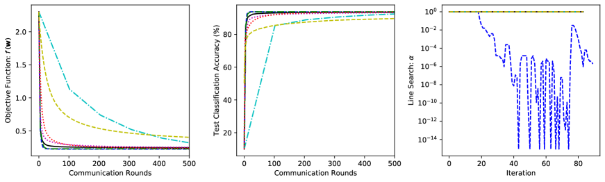
Figure 1: Softmax regression problem on the EMNIST Digits dataset. SVRG, in InexactDANE, and SGD both have a learning rate of $10^{-1}$ and AIDE has $\tau=1$. Here, we have five worker nodes, i.e., $m=5$ in (1).

The PL inequality has become widely recognized in both optimization and machine learning literature [28]. The class of functions satisfying the condition contains strongly-convex functions as a sub-class and contains functions that are non-convex [26]. This inequality has shown significant potential in the analysis of over-parameterized problems and is closely related to the property of interpolation [29, 30]. Functions satisfying (14) are a subclass of invex functions [31]. Invexity is a generalization of convexity and was considered by DINGO. Linear MLP and some linear ResNet are known to satisfy the PL inequality [32].

4 Experiments

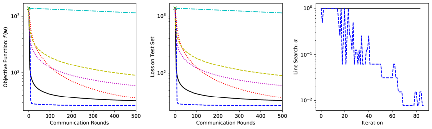
Figure 2: Non-linear least-squares problem on the CIFAR10 dataset. SVRG, in InexactDANE, and SGD have a learning rate of $10^{-4}$ and $10^{-3}$, respectively, and AIDE has $\tau=100$. GIANT failed immediately. Here, we have 50 worker nodes, i.e., $m=50$ in (1).

In this section, we examine the empirical performance of DINO in comparison to the, previously discussed, distributed second-order methods DINGO, DiSCO, GIANT, InexactDANE and AIDE. We also compare these to synchronous SGD [27]. In all experiments, we consider (1) with (2), where $S_{1},\ldots,S_{m}$ partition $\{1,\ldots,n\}$ with each having equal size $n/m$. In Table 3 and Figure 1, we compare performance on the strongly convex problem of softmax cross-entropy minimization with regularization on the EMNIST Digits dataset. In Figure 2, we consider the non-convex problem of non-linear least-squares without regularization on the CIFAR10 dataset with $\ell_{j}({\bf w};{\bf x}_{j})=\big{(}y_{j}-\log(1+\exp{\langle{\bf w},{\bf x}_{j}\rangle})\big{)}^{2}$ in (2), where $y_{j}$ is the label of ${\bf x}_{j}$. Although GIANT and DiSCO require strong convexity, we run them on this problem and indicate, with an “$\times$” on the plot, if they fail.

We first describe some of the implementation details. The sub-problems of DINO, DINGO, DiSCO, GIANT and InexactDANE are limited to 50 iterations, without preconditioning. For DINO, we use the well known iterative least squares solvers LSMR [33] and CG to approximate ${\bf v}_{t,i}^{(1)}$ and ${\bf v}_{t,i}^{(2)}$ in Algorithm 1, respectively. For DINO, and DINGO as in [20], we use the hyper-parameters $\theta=10^{-4}$ and $\phi=10^{-6}$. For DINO, DINGO and GIANT we use distributed backtracking line-search to select the largest step-size in $\{1,2^{-1},\ldots,2^{-50}\}$ that passes, with an Armijo line-search parameter of $10^{-4}$. For InexactDANE, we set the hyper-parameters $\eta=1$ and $\mu=0$, as in [19], which gave high performance in [18]. We also use the sub-problem solver SVRG [34] and report the best learning rate from $\{10^{-5},\ldots,10^{5}\}$. We let AIDE call only one iteration of InexactDANE, which has the same parameters as the stand-alone InexactDANE algorithm. We also report the best acceleration parameter, $\tau$ in [19], from $\{10^{-5},\ldots,10^{5}\}$. For SGD, we report the best learning rate from $\{10^{-5},\ldots,10^{5}\}$ and at each iteration all workers compute their gradient on a mini-batch of $n/(5m)$ data points.

The run-time is highly dependent on the distributed computing environment, which is evident in Table 3. Here, we run the methods on a single node on our local compute cluster. We also run them over a distributed environment comprised of six Amazon Elastic Compute Cloud instances via Amazon Web Services (AWS). These instances are located in Ireland, Ohio, Oregon, Singapore, Sydney and Tokyo. This setup is to highlight the effect of communication costs on run-time. As can be seen in Table 3, the second-order methods experience a notable speedup when going to the more powerful AWS setup, whereas SGD experiences a slowdown. DINO, DINGO and GIANT performed the most local computation in our experiments and they also had the largest increase in iterations. Similar behaviour to that in Table 3 can also be observed for the non-linear least-squares problem.

In Figures 1 and 2, we compare the number of communication rounds required to achieve descent. We choose communication rounds as the metric, as time is highly dependent on the network. DINO is competitive with the other second-order methods, which all outperform SGD. Recall that InexactDANE and AIDE are difficult to tune. Between Figures 1 and 2, notice the significant difference in the selected learning rate for SVRG of InexactDANE and the acceleration parameter of AIDE. Meanwhile, DINO and DINGO have consistent performance, despite not changing hyper-parameters.

In the non-convex problem in Figure 2, GIANT fails immediately as CG fails on all 50 worker nodes. DiSCO does not fail and has poor performance. This suggests that locally around the initial point ${\bf w}_{0}$, the full function $f$ is exhibiting convexity, while the local functions $f_{i}$ are not. Moreover, in Figure 2 the dimension $d$, which is $3072$, is larger than the number of training samples, $1000$, on each worker node.

5 Conclusion and Future Work

In the context of centralized distributed computing environment, we present a novel distributed Newton-type method, named DINO, which enjoys several advantageous properties. DINO is guaranteed to converge under minimal assumption, its analysis is simple and intuitive, it is practically parameter free, and it can be applied to arbitrary non-convex functions and data distributions. Numerical simulations highlight some of these properties.

The following is left for future work. First, characterizing the relationship between the hyper-parameters $\theta$ and $\phi$ of DINO. As was discussed, they have intuitive effects on the algorithm and they are easy to tune. However, there is a non-trivial trade off between them that will be explored in future work. Second, analysing the connection between DINO and over-parameterized problems. Finally, extending the theory of DINO to alternative forms of line search, such as having each worker perform local line search and then aggregating this information in a way that preserves particular properties.

References

• [1] Naman Agarwal, Ananda Theertha Suresh, Felix Xinnan Yu, Sanjiv Kumar, and Brendan McMahan. cpSGD: communication-efficient and differentially-private distributed SGD. In Advances in Neural Information Processing Systems, pages 7564–7575, 2018.
• [2] Yuchen Zhang and Xiao Lin. DiSCO: distributed optimization for self-concordant empirical loss. In International Conference on Machine Learning, pages 362–370, 2015.
• [3] Alec Radford, Jeffrey Wu, Rewon Child, David Luan, Dario Amodei, and Ilya Sutskever. Language models are unsupervised multitask learners. 2019.
• [4] Seunghak Lee, Jin Kyu Kim, Xun Zheng, Qirong Ho, Garth A Gibson, and Eric P Xing. On model parallelization and scheduling strategies for distributed machine learning. In Advances in neural information processing systems, pages 2834–2842, 2014.
• [5] Adam Paszke, Sam Gross, Soumith Chintala, Gregory Chanan, Edward Yang, Zachary DeVito, Zeming Lin, Alban Desmaison, Luca Antiga, and Adam Lerer. Automatic differentiation in PyTorch. 2017.
• [6] Martin Abadi, Paul Barham, Jianmin Chen, Zhifeng Chen, Andy Davis, Jeffrey Dean, Matthieu Devin, Sanjay Ghemawat, Geoffrey Irving, Michael Isard, Manjunath Kudlur, Josh Levenberg, Rajat Monga, Sherry Moore, Derek G. Murray, Benoit Steiner, Paul Tucker, Vijay Vasudevan, Pete Warden, Martin Wicke, Yuan Yu, and Xiaoqiang Zheng. Tensorflow: A system for large-scale machine learning. In 12th USENIX Symposium on Operating Systems Design and Implementation (OSDI 16), pages 265–283, 2016.
• [7] Ohad Shamir and Nathan Srebro. Distributed stochastic optimization and learning. In 2014 52nd Annual Allerton Conference on Communication, Control, and Computing (Allerton), pages 850–857. IEEE, 2014.
• [8] Mu Li, David G Andersen, Alexander J Smola, and Kai Yu. Communication efficient distributed machine learning with the parameter server. In Advances in Neural Information Processing Systems, pages 19–27, 2014.
• [9] Jianqiao Wangni, Jialei Wang, Ji Liu, and Tong Zhang. Gradient sparsification for communication-efficient distributed optimization. In Advances in Neural Information Processing Systems, pages 1299–1309, 2018.
• [10] John Shalf, Sudip Dosanjh, and John Morrison. Exascale computing technology challenges. In High Performance Computing for Computational Science – VECPAR 2010, pages 1–25, Berlin, Heidelberg, 2011. Springer Berlin Heidelberg.
• [11] Farzin Haddadpour, Mohammad Mahdi Kamani, Mehrdad Mahdavi, and Viveck Cadambe. Trading redundancy for communication: speeding up distributed SGD for non-convex optimization. In International Conference on Machine Learning, pages 2545–2554, 2019.
• [12] Nikita Ivkin, Daniel Rothchild, Enayat Ullah, Ion Stoica, Raman Arora, et al. Communication-efficient distributed SGD with sketching. In Advances in Neural Information Processing Systems, pages 13144–13154, 2019.
• [13] Thijs Vogels, Sai Praneeth Karimireddy, and Martin Jaggi. PowerSGD: practical low-rank gradient compression for distributed optimization. In Advances in Neural Information Processing Systems, pages 14236–14245, 2019.
• [14] Debraj Basu, Deepesh Data, Can Karakus, and Suhas Diggavi. Qsparse-local-SGD: distributed SGD with quantization, sparsification and local computations. In Advances in Neural Information Processing Systems, pages 14668–14679, 2019.
• [15] Yunfei Teng, Wenbo Gao, Francois Chalus, Anna E Choromanska, Donald Goldfarb, and Adrian Weller. Leader stochastic gradient descent for distributed training of deep learning models. In Advances in Neural Information Processing Systems, pages 9821–9831, 2019.
• [16] Shuai Zheng, Ziyue Huang, and James Kwok. Communication-efficient distributed blockwise momentum SGD with error-feedback. In Advances in Neural Information Processing Systems, pages 11446–11456, 2019.
• [17] Shusen Wang, Farbod Roosta, Peng Xu, and Michael W. Mahoney. GIANT: globally improved approximate Newton method for distributed optimization. In Advances in Neural Information Processing Systems, pages 2338–2348, 2018.
• [18] Ohad Shamir, Nati Srebro, and Tong Zhang. Communication-efficient distributed optimization using an approximate Newton-type method. In International Conference on Machine Learning, pages 1000–1008, 2014.
• [19] Sashank J. Reddi, Jakub Konečnỳ, Peter Richtárik, Barnabás Póczós, and Alex Smola. AIDE: fast and communication efficient distributed optimization. arXiv preprint arXiv:1608.06879, 2016.
• [20] Rixon Crane and Fred Roosta. DINGO: distributed Newton-type method for gradient-norm optimization. In Advances in Neural Information Processing Systems, pages 9494–9504, 2019.
• [21] Shashi K. Mishra and Giorgio Giorgi. Invexity and Optimization. Springer Berlin Heidelberg, Berlin, Heidelberg, 2008.
• [22] Farbod Roosta and Michael W Mahoney. Sub-sampled Newton methods. Mathematical Programming, 174(1-2):293–326, 2019.
• [23] Peng Xu, Farbod Roosta, and Michael W Mahoney. Newton-type methods for non-convex optimization under inexact Hessian information. Mathematical Programming, 2019. doi:10.1007/s10107-019-01405-z.
• [24] Nicol N Schraudolph. Fast curvature matrix-vector products for second-order gradient descent. Neural computation, 14(7):1723–1738, 2002.
• [25] Jorge Nocedal and Stephen Wright. Numerical Optimization. Springer Science & Business Media, 2006.
• [26] Hamed Karimi, Julie Nutini, and Mark Schmidt. Linear convergence of gradient and proximal-gradient methods under the Polyak-Łojasiewicz condition. In Machine Learning and Knowledge Discovery in Databases, pages 795–811, Cham, 2016. Springer International Publishing.
• [27] Jianmin Chen, Rajat Monga, Samy Bengio, and Rafal Jozefowicz. Revisiting distributed synchronous SGD. In International Conference on Learning Representations Workshop Track, 2016.
• [28] Yunwen Lei, Ting Hu, Guiying Li, and Ke Tang. Stochastic gradient descent for nonconvex learning without bounded gradient assumptions. IEEE Transactions on Neural Networks and Learning Systems, pages 1–7, 2019.
• [29] Raef Bassily, Mikhail Belkin, and Siyuan Ma. On exponential convergence of sgd in non-convex over-parametrized learning. arXiv preprint arXiv:1811.02564, 2018.
• [30] Sharan Vaswani, Aaron Mishkin, Issam Laradji, Mark Schmidt, Gauthier Gidel, and Simon Lacoste-Julien. Painless stochastic gradient: Interpolation, line-search, and convergence rates. In Advances in Neural Information Processing Systems, pages 3727–3740, 2019.
• [31] Fred Roosta, Yang Liu, Peng Xu, and Michael W. Mahoney. Newton-MR: Newton’s method without smoothness or convexity. arXiv preprint arXiv:1810.00303, 2018.
• [32] Yasutaka Furusho, Tongliang Liu, and Kazushi Ikeda. Skipping two layers in resnet makes the generalization gap smaller than skipping one or no layer. In INNS Big Data and Deep Learning conference, pages 349–358. Springer, 2019.
• [33] David Chin-Lung Fong and Michael Saunders. LSMR: an iterative algorithm for sparse least-squares problems. SIAM Journal on Scientific Computing, 33(5):2950–2971, 2011.
• [34] Rie Johnson and Tong Zhang. Accelerating stochastic gradient descent using predictive variance reduction. In Advances in Neural Information Processing Systems, pages 315–323, 2013.