Flares in the Galactic center I: orbiting flux tubes in Magnetically Arrested Black Hole Accretion Disks
Abstract
Recent observations of SgrA* by the GRAVITY instrument have astrometrically tracked infrared flares (IR) at distances of gravitational radii (). In this paper, we study a model for the flares based on 3D general relativistic magneto-hydrodynamic (GRMHD) simulations of magnetically arrested accretion disks (MADs) which exhibit violent episodes of flux escape from the black hole magnetosphere. These events are attractive for flare modeling for several reasons: i) the magnetically dominant regions can resist being disrupted via magneto-rotational turbulence and shear, ii) the orientation of the magnetic field is predominantly vertical as suggested by the GRAVITY data, iii) magnetic reconnection associated with the flux eruptions could yield a self-consistent means of particle heating/acceleration during the flare events. In this analysis we track erupted flux bundles and provide distributions of sizes, energies and plasma parameter. In our simulations, the orbits tend to circularize at a range of radii from . The magnetic energy contained within the flux bundles ranges up to , enough to power IR and X-ray flares. We find that the motion within the magnetically supported flow is substantially sub-Keplerian, in tension with the inferred period-radius relation of the three GRAVITY flares.
keywords:
black hole physics – accretion, accretion discs – magnetic reconnection – MHD – methods: numerical1 Introduction
Near infrared (NIR) observations of the Galactic center have provided an exciting number of discoveries: foremost the precise measurement of the Galactic Center black hole mass and distance of and through astrometric monitoring of stellar orbits Schödel et al. (2002); Ghez et al. (2003); Gravity Collaboration et al. (2019). Furthermore, the gravitational redshift and post-Newtonian orbit of S2 star was recently measured (Gravity Collaboration et al., 2018a, 2020) setting tight bounds on the compactness of the central mass.
In addition to precision measurements of stellar orbits, NIR monitoring has revealed recurring flux increase flares which last for around an hour and occur roughly four times per day (Genzel et al., 2003). The peak intensity is and the emission is strongly polarized with changing polarization angle during the flare (Eckart et al., 2006; Trippe et al., 2007; Shahzamanian et al., 2015). Besides IR flares, the Galactic Center is also prone to simultaneous X-ray flares, albeit only one in four IR flares also has an X-ray counterpart (Baganoff et al., 2001; Porquet et al., 2003; Hornstein et al., 2007). The IR flares (but not the X-ray flares) exhibit substructure down to minute and large structural variations on timescales of minutes (Dodds-Eden et al., 2009; Do et al., 2009). These observations suggest a synchrotron origin of the IR emission from a compact region of size within from the black hole Broderick & Loeb (2005); Witzel et al. (2018).
Recently, the GRAVITY collaboration has reported three bright flares and astrometrically tracked their flux centroids with an accuracy of (Gravity Collaboration et al., 2018b, in the following: G18). The centroid positions and polarization swings with periods of minutes were found to be compatible with a relativistic Keplerian circular orbit at (The GRAVITY Collaboration et al., 2020). A striking feature of these observations is that the polarization signature implies a strong poloidal component of the magnetic field in the emitting region (G18).
GRMHD simulations of radiatively inefficient accretion are quite successful in reproducing many aspects of the galactic center such as spectra, source sizes, some aspects of variability and polarization signatures, yet no consensus model reproduces all observables at once (Mościbrodzka et al., 2009; Dexter et al., 2010; Dibi et al., 2012; Mościbrodzka & Falcke, 2013; Chan et al., 2015a; Ressler et al., 2016; Gold et al., 2017; Chael et al., 2018; Anantua et al., 2020). In the IR, large uncertainties are present due to the necessity of including electron heating and likely non-thermal processes in the radiative models (Chael et al., 2017; Chael et al., 2018; Davelaar et al., 2018).
Before exploring this large and uncertain parameter space, we here focus on the dynamics that could initiate IR flares like the ones observed by G18. In the context of the G18 flares, simulations of magnetically arrested disks (MAD) (Igumenshchev et al., 2003; Tchekhovskoy et al., 2011; McKinney et al., 2012) are particularly promising: The simulations show frequent eruptions of excess magnetic flux from the saturated black hole magnetosphere. As first described by Igumenshchev (2008), these flux bundles appear as highly magnetised “blobs” with a dominant poloidal magnetic field component in the accretion disk (e.g. Avara et al., 2016; Marshall et al., 2018; White et al., 2019). Once the excess flux is re-accreted, a repeating quasi-periodic cycle of outbursts from the black hole is set up.
The environment in which these eruptions occur is turbulent and complex and the mechanism behind the flux escape events is somewhat uncertain. Yet the process is reminiscent of a Rayleigh-Taylor-like interchange between funnel- and disk-plasma which is triggered once the accumulated magnetic pressure overcomes the ram pressure of the accretion stream (see e.g. the discussion in Marshall et al., 2018). Magnetic reconnection might be involved to promote accretion through the magnetic barrier (Igumenshchev et al., 2003) or to change topology of funnel field lines through a Y-point in the equatorial plane.
Large-scale simulations of mass feeding in the Galactic Center through magnetised stellar winds have recently been presented by Ressler et al. (2019, 2020). They demonstrate that for a wide range of initial wind magnetisations, the (extrapolated) horizon scale magnetic field is of order of the MAD limit. Similar to MAD accretion, the inner magnetic field is dominated by the polodial component and magneto-rotational instability (MRI) is either marginally or fully suppressed. This serves as additional strong motivation to study MAD dynamics in context of SgrA* flares.
The paper is organized as follows: in section 2 we first describe the GRMHD simulations and analyze timing properties of various diagnostics in the simulations. We then elucidate on the flux eruption mechanism and describe our method of flux tube selection for the following statistical analysis. We conclude in section 3.
2 Results
2.1 Overall characteristics of the simulations
In this paper, we discuss GRMHD simulations obtained with BHAC (Porth et al., 2017; Olivares et al., 2019) 111https://www.bhac.science using modified Kerr-Schild coordinates (McKinney & Gammie, 2004) and 2–3 levels of static mesh refinement. Unless stated explicitly, we use units where , which for instance sets the length unit , where is the mass of the black hole. The simulations are initialised with a hydrodynamic equilibrium torus following Fishbone & Moncrief (1976) with inner edge at and density maximum at and we use an ideal equation of state with an adiabatic index of . We perturb the initial state by adding a purely poloidal magnetic field capable of saturating the black hole flux. The particular vector potential reads:
| (1) |
where subscript indicates ordinary Kerr-Schild coordinates. The initial magnetic field is weak and scaled such that the ratio of pressure maxima adopts a value of .
| ID | a | |||
|---|---|---|---|---|
| MAD-128 | ||||
| MAD-192 | ||||
| MAD-192-CR | ||||
| SANE-256 |
An overview of the simulations used in this paper is given in Table 1. With the fiducial (dimensionless) spin value of , we discuss two MAD cases with increasing resolutions and one standard and normal evolution (SANE) case for comparison. In addition, a counter-rotating case with is shown to investigate the spin dependence of the results. To check for convergence of the simulations, we quote the mass-weighted MRI quality factors (Q-factors, see section 2.3) also in Table 1. As indicated by Q-factors above 10, all simulations have sufficient resolution to capture the magneto-rotational instability (e.g. Hawley et al., 2011; Hawley et al., 2013; Sorathia et al., 2012).
2.2 Time series
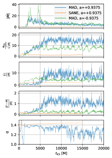
A time-series of horizon penetrating fluxes following the definitions of Porth et al. (2019) is shown in Figure 1. A quasi-stationary MAD state is obtained after , where the dimensionless horizon penetrating magnetic flux reaches the critical value of for and for , consistent with Tchekhovskoy et al. (2012) 222In our system of units, which differs from the commonly employed definition of Tchekhovskoy et al. (2011, 2012); McKinney et al. (2012) by a factor of ). Quasi-periodic dips in the horizon penetrating magnetic flux are visible in particular in the counter-rotating case where up to half of the flux is expelled in strong events. The flux is then re-accreted and the expulsion repeats after a timescale of which corresponds to hours in the galactic center. In the co-rotating case, we see weaker flux expulsions and correspondingly the timescale of re-accretion is considerably shorter. The normalized accretion power measured at the event horizon, , shows an efficiency of up to , indicating the extraction of spin-energy and is a characteristic property of the MAD state (Tchekhovskoy et al., 2012).
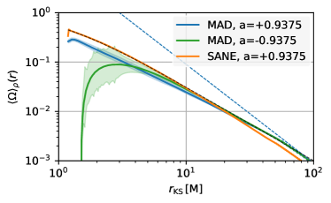
Turning to the rotation profiles which are given through the powerlaw:
| (2) |
with index . While the SANE case is compatible with Keplerian motion (), once large flux tubes appear around , the MAD case becomes substantially sub-Keplerian () due to additional magnetic support. The rotation and shear will be analyzed further in section 2.6.
It is interesting to consider how accretion of mass and magnetic flux are inter-related for MAD disks. Naively, if accretion proceeds through an interchange process, one might expect and to be anti-correlated. This is because dense plasma (increasing ) is “interchanged” with strongly magnetised funnel plasma (decreasing ). However, as pointed out also by Beckwith et al. (2009), the black hole mass must increase, whereas magnetic flux can also decrease due to “escape” from the black hole and due to the accretion of opposite polarity field lines and reconnection. Hence it is not clear whether a correlation between the two properties should exist at all, as different processes might govern their respective evolutions.
To analyze the accretion process, as a first step, we investigate the auto-correlation of the rates of mass , energy- and angular- momentum and as well as the rate of magnetic flux increase . The correlation time is defined as the lag when the autocorrelation assumes a value of and the time-series is restricted to a time when the simulations are firmly in the MAD state: . This yields a correlation time for the (detrended) of for the fiducial runs MAD-128 and MAD-192, respectively. These values are consistent with the decorrelation time of the ray-traced synthetic images used in the EHT model fitting (Event Horizon Telescope Collaboration et al., 2019). Repeating this analysis for and yields similar results. Quite in contrast to and , it turns out that in our simulations is uncorreltated down to the sampling frequency of , both for the MAD and SANE cases. Accordingly, there is no detectable correlation between mass accretion and . This is a strong indication that the black hole flux in the saturated state is subject to a highly intermittent random process and does not follow the long-term trends seen in the accretion of mass.
We have further checked for cross-correlations between the aforementioned quantities and note one striking difference between the SANE and MAD cases: in turbulent SANE accretion, the time-series of and are clearly anti-correlated, meaning low density streams of gas carry higher than average specific angular momentum. The MAD cases show no clear correlation. A possible interpretation could be: if angular momentum of low-density flux tubes is removed via large scale stresses in MAD accretion, it is expected that these low density flux tubes carry systematically lower angular momentum when they are accreted. Hence one would expect a positive correlation between and . If both turbulent MRI accretion and flux tube accretion occur at the same time, likely no correlation is observed.
2.3 Flux tube selection
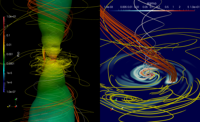
Flux tubes are dominated by coherent large scale vertical magnetic fields. They differ substantially from the MRI active regions where the field is sub-dominant and its geometry is mostly toroidal. This is visualized in Figure 2, where we chose footpoints rooted on: the black hole event horizon (white field lines), in the MRI active turbulent disk (yellow lines), and in a high-magnetization region in the equatorial plane (red). Here we introduce the (hot-) magnetization which compares the square of the fluid-frame field strength and the enthalpy density of the gas . Within one scale height of the disk, the flux tube remains nearly vertical and is subsequently wound up around the jet. Its mid-plane magnetization is and, as the field is strong, the MRI is quenched in the flux tube.
The suppression of the MRI is quantified by the “MRI suppression factor” which compares the disk scale-height with the wavelength of the fastest growing (vertical) MRI mode . No growth is expected for wavelengths that do not “fit” into the disk diameter, hence for . For a quantitative analysis, we define the density weighted averages as:
| (3) |
| (4) |
with denoting the quantity being averaged, is the determinate of the four-metric, and where we set an averaging interval in the quasi stationary state , . We measure the (density-) scale height as
| /Hr | (5) |
The fastest growing mode is evaluated in a co-moving orthonormal reference frame (Takahashi, 2008) as:
| (6) |
where is the coordinate angular velocity of the fluid. We define the average suppression factor as:
| (7) |
and the MRI quality factors as:
| (8) |
The mass-weighted averages of the Q-factors within are noted for each run in Table 1.
Effectively, the suppression factor means that MRI does not grow in magnetically dominated regions. This can be seen using the thin disk relation and noting that is the vertical Alfvén velocity. Hence
| (9) |
simply compares the sound- and Alfvén- velocities or magnetic and thermal pressure contributions.
To identify flux tubes for further analysis, we therefore look for regions with dominant vertical field component and trace the contours where in the equatorial plane. In addition, to reduce the level of noise in the detection, we restrict our analysis to flux tubes with a cross-section of at least in area, where is the radius of the black hole event horizon. We have verified, using these criteria, that for the SANE case this comparison does not show any flux tubes.
Figure 3 illustrates the properties of these regions for three consecutive times for simulation MAD-128. The flux tubes selected in this fashion have dominant out-of-plane magnetic fields which were checked by tracing their field lines as in Figure 2 for several selected cases. Figure 3 shows that flux tubes coincide with suppressed MRI (top panels), and have low plasma- and higher than average , as expected (bottom two rows).
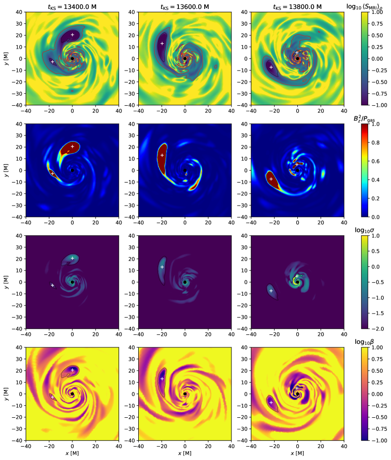
It is interesting to note that in both runs MAD-128 and MAD-192, we find that the angle- and time- averaged suggests MRI suppression within . However, within this radius, dense streams of accreting material are frequently found where the MRI can in principle operate.
2.4 Dynamics of flux tubes
Over time, a flux tube will become more elongated as it shears out in the differentially rotating accretion flow. Flux- and mass- conservation for constant scale height yields a simple estimate for the pressure contributions in the flux tube:
| (10) | ||||
| (11) |
where is a measure of the size of the flux tube (here defined as the radius of the circle having the same surface as the cross-sectional area of the flux tube). Hence for any causal , the magnetic pressure decreases faster than the thermal pressure as the flux tube increases in size. As the flux tube moves outwards, the ambient pressure decreases and pressure equilibrium is obtained via expansion of the tube, hence the flux tube expands and looses its magnetic dominance. Shear- and Rayleigh-Taylor induced mixing can also increase the size of the flux tube over time. Once distributed over a large area, the flux tube cannot remain magnetically dominated and is dissipated in the accretion flow.
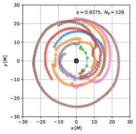
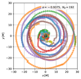
To analyze the motion of the flux tubes, we compute the centroid of the magnetic flux in the selected magnetically dominated regions in the equatorial plane, illustrated by “” signs in Figure 3. The centroid motions of robust features which can be tracked for at least one quarter of a circle are illustrated in Figure 4. A flux bundle spirals outwards to eventually circularize at what we call its “circularization radius”. For different flux tubes we recover different circularization radii ranging up to . Over the considered time interval , the high-resolution MAD-192 case shows fewer eruptions than MAD-128, yet the parameters of the present features are comparable.
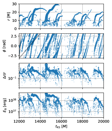
Key parameters of the flux tube evolution are summarized in Figure 5 where we show the coordinate values , the relative size of the magnetically dominated region, , and the magnetic energy contained within one density scale height, . To compute the normalization for the latter, we perform ray-tracing radiative transfer of the data using the BHOSS code (Younsi & Wu (2015), Younsi et al. 2020) and scale the simulations to recover the Galactic Center flux of observed at an EHT frequency of (Doeleman et al., 2008). We apply an inclination of and “standard parameters” from the M87 modeling (Event Horizon Telescope Collaboration et al., 2019): and adopt a high-sigma cutoff .
By tracing the radius and azimuth, it is seen that flux tubes generally move outwards from the black hole due to the magnetic tension of the highly pinched fields and slow down their radial motion to orbit at constant radius between and . As flux tubes are eroded by the ambient flow and decrease in magnetization, just before they dissolve, the detected (radial-) centroid motions become erratic. This is reflected in the first panel of Figure 5 as seemingly inward- or outward moving features observed after circularization. The large variance in circularization radii indicates that the final resting place of the flux bundles is not given by the magnetospheric radius (which on average lies ). Rather, we find that when the field enters a circular orbit it has also adopted a predominantly vertical orientation and hence no tension force is available to drive it out further.
Orbital periods between and are recovered in our simulations, depending on the radial location of the fields. Due to the increase of plasma- (and thus decrease of the tracer quantity ), the inferred size and magnetic energy gradually decrease until the flux tube is no longer detected as a magnetically-dominated region. At its maximum, the magnetic energy reaches for both the MAD-128 and MAD-192 simulations.
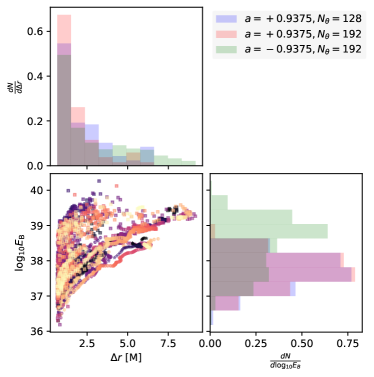
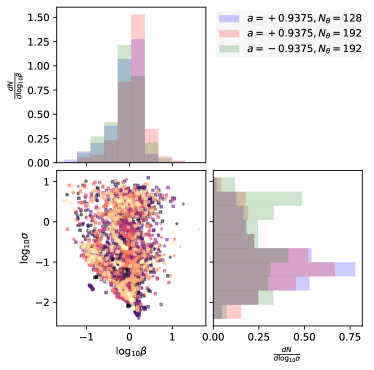
2.5 Distributions
The instantaneous distributions of various flux tube properties are shown in Figure 6. Small flux tubes with close to the detection cutoff dominate in number, but sizes of up to are recovered. As shown in the top panel of Figure 6, the range of magnetic energies span over two orders of magnitude, from to in the co-rotating case and ranging up to in the counter-rotating case. The most probable magnetic energy of a flux tube is (co-rotating) respectively (counter-rotating) and large flux tubes are only found with high magnetic energies. However, smaller flux tubes are found at all magnetic energies.
Turning to the average plasma- and magnetisation of the flux tubes, the distribution of plasma- peaks close to the detection threshold but extends down to . The magnetisations start at with the peak at and an extended tail ranging up to . The counter-rotating case has a broader distribution of with a second peak at . Efficient particle acceleration via magnetic reconnection requires the plasma to be magnetically dominated, hence and . In our sample, we find that this is the case for of the identified features. We have carried out this analysis for both MAD-128 and MAD-192 runs, finding that these results are quite insensitive to the choice of resolution and run.
2.6 Shearing analysis
As in any differentially rotating flow, azimuthally advected features are destined to wind up and loose their coherence. Naturally, while magnetically dominated and subject to large scale tension force, flux bundles are not readily sheared however. In some sense, they behave more like the spoon that stirs the tea rather than the milk in it. Over time however, they will loose magnetic dominace (see Section 2.4) and it is instructive to consider how long such “passive tracers” can remain coherent in a given differential rotation profile. This should provide a lower limit to the survival of the flux tubes against shear. Given a rotation law of the form (2), for a feature contained within , the inner edge will “lap” the slower moving outer component after one shearing timescale:
We show the rotation profile of the simulations in Figure 7. In the SANE case, the rotation in the inner quasi-stationary regions is described by a relativistic Keplerian motion (dashed black curve) which is fitted by a powerlaw for with . Due to additional magnetic support, the inner regions of the co-rotating MAD case are sub-Keplerian with a shallower powerlaw index of . In the counter-rotating case, large departures from Keplerian motion are observed within the ISCO of and the violent ejection of large flux bundles reflects the large variance of the rotation profile within .
Varying in the range , however, does not significantly alter the shearing timescale. This means that small features with can in principle survive for orbital periods, whereas large features with would be smeared out after roughly one orbit. For the majority of the detected features with relative sizes , differential rotation allows several orbits before the features would be fully smeared out due to shear.
2.7 Orbital periods
The three astrometrically tracked flares from 2018 reported by Gravity Collaboration et al. (2018b) have shown motion on scales of . Although only one orbit appears closed, within the measurement errors, all three flares can be explained by a single Keplerian circular orbit with a radius of (The GRAVITY Collaboration et al., 2020). While not statistically significant, (The GRAVITY Collaboration et al., 2020) note that the sizes of the flux centroid motions appear to be systematically larger than the model predictions. In other words, the model Keplerian motion at the observed centroid position is too slow compared to the observational data. Recently, Matsumoto et al. (2020) analyzed the July 22 flare with a broader range of models including marginally bound geodesics and super-Keplerian pattern motion, confirming this finding. They also find that a super-Keplerian circular orbit with at yields a better match to the data than the Keplerian orbits. However, as the measurement errors are substantial, all models are formally acceptable at present.
With the features found in the GRMHD simulations, it is interesting to ask how their orbital periods compare to the data of the flares. To this end, we need to track features over time in the simulation data. Our algorithm works as follows: 1. with a cadence of , we obtain the boundary curves of the magnetically dominated flux tubes in the equatorial plane as described in section 2.3. 2. for two consecutive snapshots, we identify a flux tube from the second snapshot with a previously identified flux tube from the first snapshot when their surfaces contained within the two boundary curves overlap by at least . This overlap is formally computed as the surface of the intersection between normalized to their union: .
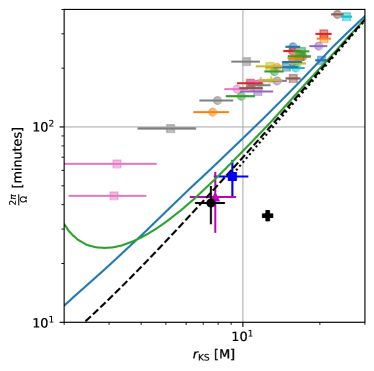
We verify that this leads to a robust tracking by visually inspecting several test cases. Figure 8 shows the (mean) orbital periods against radius for all features which can be traced for at least . To illustrate the radial evolution, we show the standard deviation of the radial coordinate as an error-bar. As comparison cases, we also overplot: 1. the datapoints from Gravity Collaboration et al. (2018b) which have been modeled as Keplerian orbits and 2. the “super-Keplerian” pattern motion fit from Matsumoto et al. (2020).
As shown by the figure, all features are significantly sub-Keplerian and are also slower than the average local rotation velocity by a factor of typically . The counter-rotating case shows an abundance of features in the inner region. These are much slower (up to times) than the average flow and exhibit strong radial variation as flux tubes are expelled with large outward velocities. Hence the fastest feature we could observe has an orbital period of . Inspecting the instantaneous coordinate velocities of the tracked features, apart from a handful of outliers due to small uncertainties in tracking, here we also do not find any evidence for super-Keplerian motion in the centroid motions. Therefore, as MAD flows have generically sub-Keplerian rotation profiles (Igumenshchev et al., 2003) and flux tubes tend to “lag behind” even further due to the magnetic torques exerted by them (Spruit & Uzdensky, 2005; Igumenshchev, 2008), the MAD model is in tension with the apparent observed fast rotations (respectively large radii of the centroids).
3 Discussion and Conclusions
In MAD disks, low density, high magnetisation flux bundles are frequently expelled from the black hole magnetosphere. As a candidate scenario for the astrometrically resolved flares observed by Gravity Collaboration et al. (2018b), we have analyzed the dynamics and energetics of these magnetised regions.
Since the flux bundles coincide with regions of suppressed MRI turbulence, they can remain coherent in the accretion flow for several orbital timescales. For the features identified in our simulations, orbital shear would set an upper limit of to orbits, depending on the size which varies from . In practice, a maximum of roughly two orbits was observed before features ceased to be detected as magnetically dominated regions in the accretion flow. As strongly magnetized flux tubes are stabilized by the magnetic tension, orbital shear cannot solely be responsible for the destruction of flux bundles however.
Driven outward by magnetic tension from the radially pinched fields, flux bundles initially move out radially and then follow circular orbits when the field has straightened out to an essentially vertical structure. The model can therefore explain orbiting features at a range of radii. We propose that the dissolution of the flux bundle is governed by the following two effects: as the outward moving flux bundle seeks pressure equilibrium with its surroundings, it is forced to expand which leads to a decrease of its magnetic dominance. Differential rotation and local shear induced Kelvin-Helmholtz instabilities (e.g. White et al., 2019; Antolin et al., 2014) are then available to erode the surface of the flux bundle.
By running one counter-rotating case with spin , we have checked that the flux bundles orbiting at relevant radial distances of do not depend significantly on black hole spin. Differences arise mainly within , where the counter-rotating case exhibits a steeply declining rotation profile. However, in the counter-rotating case, the flux bundles are more energetic by an order of magntitude. This results from two effects: first, the lower radiative efficiency of the counter-rotating case implies that for the same normalizing mm-flux, a higher accretion rate and density is required. Second, the eruptions found in the counter-rotating case remove a larger fraction of magnetic flux from the black hole (up to ) resulting in stronger flares.
We have computed distributions of sizes, magnetisation and energy contained within the flux bundles for the co- and counter-rotating case. When the simulations are scaled to match the flux of the Galactic Center, we find that the most probable magnetic energy in the co-rotating case is and in the counter-rotating case. The latter distribution however extends all the way up to . Given that strong flares radiate up to in X-rays (Baganoff et al., 2001; Hornstein et al., 2007; Bouffard et al., 2019), the counter-rotating case has sufficient magnetic energy to allow for a radiative efficiency of a few percent. In our sample, in of the cases, we found average plasma parameters with and , allowing for efficient particle acceleration via magnetic reconnection.
While magnetic reconnection likely plays a role in the expulsion of magnetic flux from the black hole, due to the highly-variable nature of the inner dynamics, it is difficult to identify clear signatures of a topology change of the magnetic field. Two-dimensional (resistive) GRMHD simulations of MAD disks by Ripperda et al. (2020) on the other hand have shown an episodically forming equatorial current sheet endowed with a plasmoid chain – a smoking gun of reconnection. It is an intriguing possibility that flux threading the black hole might escape via reconnecting through this equatorial current sheet as it can provide a means of loading the flux bundles with relativistic particles. In our simulations, azimuthal interchange instabilities do not allow a strong current sheet to persist and the flow is continuously perturbed by spiral stream of accreting material. The mechanism that we envision was recently also described in the context of protostellar flares by Takasao et al. (2019). In their resistive MHD simulations, reconnection in the equatorial region heats plasma associated with flux removal from the star leading to flare energies consistent with X-ray observations. Future resistive 3D GRMHD simulations will be better suited to elucidate the nature of magnetic reconnection in MAD accretion as it enables a parametric exploration of the resistivity.
An important constraint for the flaring model comes from the period-radius relation of the flares. Whereas the observations by Gravity Collaboration et al. (2018b) suggest Keplerian or even super-Keplerian motion (Matsumoto et al., 2020), since MAD disks are sub-Keplerian and flux bundles tend to lag by an additional factor of in the periods (as already pointed out by Igumenshchev (2008)), there is some tension with the current observations. In this regard, it is important to consider alternative models like the ejected plasmoids studied by Younsi & Wu (2015); Nathanail et al. (2020); Ball et al. (2020). In this model, the emission originates from outward moving plasmoids which form due to magnetic reconnection in the coronal regions of the accretion flow. The changed geometry can yield an explanation for the offset between the mean centroid position and the black hole (Ball et al., 2020) as well as reconcile the super-Keplerian motion due to finite light-travel time effects (The GRAVITY Collaboration et al., 2020). Whether the model can also explain the energetics, polarization and recurrence time of SgrA* flares remains to be seen.
It might be worthwile to briefly entertain the possibility of a “confusion scenario” to explain the apparent super-Keplerian nature of the 2018 July 22 flare: as multiple flux tubes can be present at the same time, one might wonder what are the chances that several independent flares in fact led to the observed characteristics. Our reasoning against it is as follows: if one were to observe multiple flaring tubes (not connected by some “pattern motion signal”), it is quite unlikely that 9 out of the 10 datapoints presented in G18 for the July 22 flare are monotonously increasing their azimuthal angle by a similar amount. 333 Grossly and brazenly simplifying (and dropping the first datapoint which breaks the monotonous trend): if 9 flux tubes are present at the same time and anyone can light up at any given time, only 9 out of the 9! realizations would yield the observed ordering. This one in 40 320 chance does not even include yet the minute likelyhood that 9 independent large flares are observed within 30 minutes given the average flare rate (following poissonian statistics) of around 4 per day. Of course one can argue whether truly 9 confused flares are required to explain the data or whether one could do with less. None the less, we belive the odds are strongly stacked against the confusion scenario, even more so since as G18 notes, “all three flares can in principle be accounted by the same orbit model”.
It is necessary to discuss several caveats of our analysis. To detect flux bundles, we look for regions of suppressed MRI and identify features via the ratio of in the equatorial plane. Changing the detection threshold can lead to more or less detected features altering slightly the quantitative distributions measured in Section 2.5. This has little influence, however, on the inferred motion of the magnetic flux centroid which is used for analysis of orbital periods carried out in section 2.7.
In particular for MAD simulations, which show strong magnetisations and steep gradients of plasma parameters within the disk, it is important to check the resolution-dependence of the results White et al. (2019). To this end, we have carried out two simulations of the fiducial case, differing by a factor of in resolution. We find that the results of our quantifications are generally consistent with each other and have combined both simulations to increase the available statistics of the analysis. It is so far unknown what sets the strength of the flux eruptions. Most likely, thin disks will experience stronger flares (Marshall et al., 2018), however a dependence on the initial conditions, e.g. the initial flux distribution in the disk cannot yet be ruled out.
For a direct comparison with the observational data, one needs to compute the near-IR intensity and polarization following a ray-tracing through the simulation data. This is carried out in a recent parallel effort by Dexter et al. (2020) who use a long MAD simulation lasting for and apply (thermal) electron heating from (sub-grid) magnetic reconnection models due to Werner et al. (2018). As the density in the escaping flux bundles is set by the funnel floors, emission of the flux bundles themselves is strongly suppressed. To estimate the emission from the flux bundles in our study, we have carried out the following experiment with the fiducial run: we apply a threshold to only select regions of strong vertical flux in the emitting volume. Applying the standard thermal emission model as described in Section 2.4, in particular , we obtain a contribution of to the emission and the contribution to the flux is even smaller . Raising the high-magnetization threshold to and again normalizing the accretion rate to recover the observed flux increases the total infrared emission by a factor of (from to ). For comparison: the equivalent increase found by Dexter et al. (2020) was a factor of . This increase is explained only to a very small part by the added contribution of disk-orbiting flux bundles (which have a median , e.g. Figure 6) but is largely due to the strongly magnetized plasma near the jet wall. In fact, the strong dependence of the IR emission on in MAD simulations is a known issue which was studied in detail within two-temperature simulations by Chael et al. (2019) and our results are consistent with their findings. Hence any radiation modeling of IR emission has to deal to a smaller or larger degree with the arbitrary truncation via .
As discussed by Dexter et al. (2020), when the IR emission originates from disk plasma (using ), the emission at the boundary of the flux bundles is enhanced due to increased heating. Flux bundles thus stir up the accretion flow and their motion should also govern the IR centroid on the observational plane. The model of Dexter et al. (2020) shares many features with the observed flares which raises the hope that IR flares might be explained without invoking high-magnetization material that – in simulations – is plagued by arbitrary floor values and uncertain electron thermodynamics.
None the less, the radiative modeling is still complicated by the fact that at least for strong simultaneous X-ray and IR flares, additional physics of non-thermal particle acceleration is required (Markoff et al., 2001; Dodds-Eden et al., 2009; Chan et al., 2015b; Ball et al., 2016). Purely thermal models of IR flares relying on gravitational lensing events have also been proposed (Dexter & Fragile, 2013; Chan et al., 2015b), but have difficulty in explaining the required flare amplitude and NIR spectral index. In fact, spectral modeling indicates that a non-thermal tail in the distribution function is required both in quiescence and during the flare (Davelaar et al., 2018; Petersen & Gammie, 2020). In particular the flat to inverted spectral index with during flares (Gillessen et al., 2006) is difficult to explain without invoking non-thermal particle acceleration. The “redness” of the spectra produced by thermal distributions was also noted by Dexter et al. (2020) who included reconnection particle heating yet no non-thermal contributions. One scenario that comes to mind is that flux bundles can be loaded with relativistic electrons as they violently reconnect in the equatorial region just before a flux escape event. While this one-off acceleration mechanism might encounter problems explaining X-ray emission from synchrotron electrons which require continuous injection, a telltale signature of such an event would be the outward motion of the flux centroid at the onset of the flare, before it circularises.
We plan to investigate the IR radiative signatures, foremost the flux centroid motion and polarization, incorporating various electron heating and acceleration prescriptions in a follow up publication.
Acknowledgements
The authors thank the anonymous referee for raising several interesting points to enhance the discussion of this paper. Y.M. and CMF are supported by the ERC synergy grant BlackHoleCam: Imaging the Event Horizon of Black Holes (grant number 610058). CMF is supported by the black hole Initiative at Harvard University, which is supported by a grant from the John Templeton Foundation. Z.Y. is supported by a Leverhulme Trust Early Career Fellowship. The simulations were performed on GOETHE at the CSC-Frankfurt and Iboga at ITP Frankfurt. This reasearch has made use of NASA’s Astrophysics Data System (ADS).
Data availability
The data underlying this article will be shared on reasonable request to the corresponding author.
References
- Anantua et al. (2020) Anantua R., Ressler S., Quataert E., 2020, MNRAS, 493, 1404
- Antolin et al. (2014) Antolin P., Yokoyama T., Van Doorsselaere T., 2014, ApJ, 787, L22
- Avara et al. (2016) Avara M. J., McKinney J. C., Reynolds C. S., 2016, MNRAS, 462, 636
- Baganoff et al. (2001) Baganoff F. K., et al., 2001, Nature, 413, 45
- Ball et al. (2016) Ball D., Özel F., Psaltis D., Chan C.-k., 2016, ApJ, 826, 77
- Ball et al. (2020) Ball D., Özel F., Christian P., Chan C.-K., Psaltis D., 2020, arXiv e-prints, p. arXiv:2005.14251
- Beckwith et al. (2009) Beckwith K., Hawley J. F., Krolik J. H., 2009, ApJ, 707, 428
- Bouffard et al. (2019) Bouffard É., Haggard D., Nowak M. A., Neilsen J., Markoff S., Baganoff F. K., 2019, ApJ, 884, 148
- Broderick & Loeb (2005) Broderick A. E., Loeb A., 2005, MNRAS, 363, 353
- Chael et al. (2017) Chael A. A., Narayan R., Sadowski A., 2017, MNRAS, 470, 2367
- Chael et al. (2018) Chael A., Rowan M., Narayan R., Johnson M., Sironi L., 2018, MNRAS, 478, 5209
- Chael et al. (2019) Chael A., Narayan R., Johnson M. D., 2019, MNRAS, 486, 2873
- Chan et al. (2015a) Chan C.-K., Psaltis D., Özel F., Narayan R., Saḑowski A., 2015a, ApJ, 799, 1
- Chan et al. (2015b) Chan C.-k., Psaltis D., Özel F., Medeiros L., Marrone D., Saḑowski A., Narayan R., 2015b, ApJ, 812, 103
- Davelaar et al. (2018) Davelaar J., Mościbrodzka M., Bronzwaer T., Falcke H., 2018, A&A, 612, A34
- Dexter & Fragile (2013) Dexter J., Fragile P. C., 2013, MNRAS, 432, 2252
- Dexter et al. (2010) Dexter J., Agol E., Fragile P. C., McKinney J. C., 2010, ApJ, 717, 1092
- Dexter et al. (2020) Dexter J., et al., 2020, MNRAS, 497, 4999
- Dibi et al. (2012) Dibi S., Drappeau S., Fragile P. C., Markoff S., Dexter J., 2012, MNRAS, 426, 1928
- Do et al. (2009) Do T., Ghez A. M., Morris M. R., Yelda S., Meyer L., Lu J. R., Hornstein S. D., Matthews K., 2009, ApJ, 691, 1021
- Dodds-Eden et al. (2009) Dodds-Eden K., et al., 2009, ApJ, 698, 676
- Doeleman et al. (2008) Doeleman S. S., et al., 2008, Nature, 455, 78
- Eckart et al. (2006) Eckart A., Schödel R., Meyer L., Trippe S., Ott T., Genzel R., 2006, A&A, 455, 1
- Event Horizon Telescope Collaboration et al. (2019) Event Horizon Telescope Collaboration et al., 2019, ApJ, 875, L5
- Fishbone & Moncrief (1976) Fishbone L. G., Moncrief V., 1976, ApJ, 207, 962
- Genzel et al. (2003) Genzel R., Schödel R., Ott T., Eckart A., Alexander T., Lacombe F., Rouan D., Aschenbach B., 2003, Nature, 425, 934
- Ghez et al. (2003) Ghez A. M., et al., 2003, ApJ, 586, L127
- Gillessen et al. (2006) Gillessen S., et al., 2006, in Journal of Physics Conference Series. pp 411–419, doi:10.1088/1742-6596/54/1/065, https://ui.adsabs.harvard.edu/abs/2006JPhCS..54..411G
- Gold et al. (2017) Gold R., McKinney J. C., Johnson M. D., Doeleman S. S., 2017, ApJ, 837, 180
- Gravity Collaboration et al. (2018a) Gravity Collaboration et al., 2018a, A&A, 615, L15
- Gravity Collaboration et al. (2018b) Gravity Collaboration et al., 2018b, A&A, 618, L10
- Gravity Collaboration et al. (2019) Gravity Collaboration et al., 2019, A&A, 625, L10
- Gravity Collaboration et al. (2020) Gravity Collaboration et al., 2020, A&A, 636, L5
- Hawley et al. (2011) Hawley J. F., Guan X., Krolik J. H., 2011, ApJ, 738, 84
- Hawley et al. (2013) Hawley J. F., Richers S. A., Guan X., Krolik J. H., 2013, ApJ, 772, 102
- Hornstein et al. (2007) Hornstein S. D., Matthews K., Ghez A. M., Lu J. R., Morris M., Becklin E. E., Rafelski M., Baganoff F. K., 2007, ApJ, 667, 900
- Igumenshchev (2008) Igumenshchev I. V., 2008, ApJ, 677, 317
- Igumenshchev et al. (2003) Igumenshchev I. V., Narayan R., Abramowicz M. A., 2003, ApJ, 592, 1042
- Markoff et al. (2001) Markoff S., Falcke H., Yuan F., Biermann P. L., 2001, A&A, 379, L13
- Marshall et al. (2018) Marshall M. D., Avara M. J., McKinney J. C., 2018, MNRAS, 478, 1837
- Matsumoto et al. (2020) Matsumoto T., Chan C.-H., Piran T., 2020, arXiv e-prints, p. arXiv:2004.13029
- McKinney & Gammie (2004) McKinney J. C., Gammie C. F., 2004, ApJ, 611, 977
- McKinney et al. (2012) McKinney J. C., Tchekhovskoy A., Blandford R. D., 2012, MNRAS, 423, 3083
- Mościbrodzka & Falcke (2013) Mościbrodzka M., Falcke H., 2013, A&A, 559, L3
- Mościbrodzka et al. (2009) Mościbrodzka M., Gammie C. F., Dolence J. C., Shiokawa H., Leung P. K., 2009, ApJ, 706, 497
- Nathanail et al. (2020) Nathanail A., Fromm C. M., Porth O., Olivares H., Younsi Z., Mizuno Y., Rezzolla L., 2020, arXiv e-prints, p. arXiv:2002.01777
- Olivares et al. (2019) Olivares H., Porth O., Davelaar J., Most E. R., Fromm C. M., Mizuno Y., Younsi Z., Rezzolla L., 2019, A&A, 629, A61
- Petersen & Gammie (2020) Petersen E., Gammie C., 2020, MNRAS, 494, 5923
- Porquet et al. (2003) Porquet D., Predehl P., Aschenbach B., Grosso N., Goldwurm A., Goldoni P., Warwick R. S., Decourchelle A., 2003, A&A, 407, L17
- Porth et al. (2017) Porth O., Olivares H., Mizuno Y., Younsi Z., Rezzolla L., Moscibrodzka M., Falcke H., Kramer M., 2017, Computational Astrophysics and Cosmology, 4, 1
- Porth et al. (2019) Porth O., et al., 2019, ApJS, 243, 26
- Ressler et al. (2016) Ressler S. M., Tchekhovskoy A., Quataert E., Gammie C. F., 2016, preprint (arXiv:1611.09365)
- Ressler et al. (2019) Ressler S. M., Quataert E., Stone J. M., 2019, MNRAS, 482, L123
- Ressler et al. (2020) Ressler S. M., Quataert E., Stone J. M., 2020, MNRAS, 492, 3272
- Ripperda et al. (2020) Ripperda B., Bacchini F., Philippov A., 2020, arXiv e-prints, p. arXiv:2003.04330
- Schödel et al. (2002) Schödel R., et al., 2002, Nature, 419, 694
- Shahzamanian et al. (2015) Shahzamanian B., et al., 2015, A&A, 576, A20
- Sorathia et al. (2012) Sorathia K. A., Reynolds C. S., Stone J. M., Beckwith K., 2012, ApJ, 749, 189
- Spruit & Uzdensky (2005) Spruit H. C., Uzdensky D. A., 2005, ApJ, 629, 960
- Takahashi (2008) Takahashi R., 2008, MNRAS, 383, 1155
- Takasao et al. (2019) Takasao S., Tomida K., Iwasaki K., Suzuki T. K., 2019, ApJ, 878, L10
- Tchekhovskoy et al. (2011) Tchekhovskoy A., Narayan R., McKinney J. C., 2011, MNRAS, 418, L79
- Tchekhovskoy et al. (2012) Tchekhovskoy A., McKinney J. C., Narayan R., 2012, in Journal of Physics Conference Series. p. 012040 (arXiv:1202.2864), doi:10.1088/1742-6596/372/1/012040, http://adsabs.harvard.edu/abs/2012JPhCS.372a2040T
- The GRAVITY Collaboration et al. (2020) The GRAVITY Collaboration et al., 2020, arXiv e-prints, p. arXiv:2002.08374
- Trippe et al. (2007) Trippe S., Paumard T., Ott T., Gillessen S., Eisenhauer F., Martins F., Genzel R., 2007, MNRAS, 375, 764
- Werner et al. (2018) Werner G. R., Uzdensky D. A., Begelman M. C., Cerutti B., Nalewajko K., 2018, MNRAS, 473, 4840
- White et al. (2019) White C. J., Stone J. M., Quataert E., 2019, ApJ, 874, 168
- Witzel et al. (2018) Witzel G., et al., 2018, ApJ, 863, 15
- Younsi & Wu (2015) Younsi Z., Wu K., 2015, MNRAS, 454, 3283