Probing the physical conditions and star formation processes in the Galactic HII region S305

Abstract

We present multi-scale and multi-wavelength observations of the Galactic H ii region S305, which is excited by massive O8.5V and O9.5V stars. Infrared images reveal an extended sphere-like shell (extension $\sim$7.5 pc; at $T_{\mathrm{d}}$ = 17.5–27 K) enclosing the S305 H ii region (size $\sim$5.5 pc; age $\sim$1.7 Myr). The extended structure observed in the Herschel temperature map indicates that the molecular environment of S305 is heated by the massive O-type stars. Regularly spaced molecular condensations and dust clumps are investigated toward the edges of the infrared shell, where the PAH and H₂ emission is also observed. The molecular line data show a signature of an expanding shell of molecular gas in S305. GMRT 610 and 1280 MHz continuum maps reveal overdensities of the ionized emission distributed around two O-type stars, which are surrounded by the horseshoe envelope (extension $\sim$2.3 pc). A molecular gas deficient region/cavity is identified toward the center of the horseshoe envelope, which is well traced with PAH, H₂, molecular, and dust emission. The edges of the infrared shell are found to be located in the front of the horseshoe envelope. All these outcomes provide the observational evidence of the feedback of O-type stars in S305. Moreover, non-thermal radio emission is detected in S305 with an average spectral index $\alpha\sim-0.45$. The variations in $\alpha$, ranging from $-1.1$ to 1.3, are explained due to soft synchrotron emission and either optically-thicker thermal emission at high frequencies or a suppression of the low-frequency emission by the Razin-Tsytovich effect.

1. Introduction

Massive OB-stars ($\geq 8$ M_⊙) have a profound impact on their immediate environment through the radiative and mechanical energy they inject from their formation phase until their death. Hence, these stars have the ability to trigger the birth of young stellar objects (YSOs) and young massive stars (Elmegreen & Lada, 1977; Elmegreen, 1998; Deharveng et al., 2005, 2010). However, understanding the formation mechanisms of massive OB-stars and their feedback process are still far from complete (Zinnecker & Yorke, 2007; Tan et al., 2014). In the literature, one can find two major triggered star formation scenarios concerning the expansion of the H ii regions, which are the radiation-driven implosion (RDI; see Bertoldi, 1989; Lefloch & Lazareff, 1994) and the “collect and collapse” (see Elmegreen & Lada, 1977; Whitworth et al., 1994; Dale et al., 2007). In the RDI model, the expansion of an H ii region initiates the instability and helps in the collapse of a pre-existing dense region in the molecular cloud. In the “collect and collapse” scenario, the expansion of an H ii region collects a massive and dense shell of cool neutral material between the ionization and the shock fronts, where star formation is initiated when this material becomes gravitationally unstable; the formation of massive stars is expected in this particular scenario (e.g., Deharveng et al., 2010). These theoretical models are observationally difficult to assess. One can find the details of the observational challenges and difficulties for searching true sites of triggered star formation in Dale et al. (2015). Some indirect evidences of triggering have been reported in the literature (e.g., Deharveng et al., 2005, 2010).

In this paper, we have selected the Galactic H ii region Sh 2-305 (hereafter, S305), which is located at a distance of $\sim 3.7$ kpc (Pandey et al., 2020). Based on the previously published mid-infrared (MIR) images, S305 can be considered as a good example of a MIR bubble (see Figure 1 in Pandey et al., 2020). Approximately at its center, S305 harbors two spectroscopically identified massive O-type stars (O8.5V: VM4 and O9.5V: VM2; Vogt & Moffat, 1975; Chini & Wink, 1984; Russeil et al., 1995; Pandey et al., 2020). In the direction of S305, the ionized gas was traced in a radial velocity of $\sim 35.4$ km s^-1 (e.g., Balser et al., 2011; Hou & Han, 2014). Using the James Clerk Maxwell Telescope (JCMT) ¹²CO(2–1) and ¹³CO(2–1) line data, Azimlu & Fich (2011) studied the properties of molecular clouds associated with 10 H ii regions including S305, and the molecular gas toward S305 was examined in a velocity range of about 42–49 km s^-1 (see Tables 2 and 3 in their paper). Using optical and infrared (IR) photometric data, Pandey et al. (2020) identified and studied the distribution of 116 YSOs in S305 in an area of $\sim 18.5\arcmin\times 18.5\arcmin$. These authors observed at least three stellar sub-clusterings in S305 (see Figure 3 in their paper). One of the clusters is detected toward the center of S305, which spatially coincides with the previously known young open star cluster “Mayer 3” (Vogt & Moffat, 1975; Chini & Wink, 1984; Russeil et al., 1995). The site S305 was mapped in the JCMT SCUBA2 450 and 850 $\mu$m continuum maps, and several clumps were observed in S305 (see Figure 5 in Sreenilayam et al., 2014). Using the Herschel column density map (resolution $\sim 12\arcsec$), at least 25 clumps (mass range $\sim$35–1565 M_⊙) have been reported in S305, and star formation activities are traced at some of these clumps (e.g., Pandey et al., 2020). Pandey et al. (2020) suggested that the two massive O-type stars might have stimulated the birth of young stars in S305.

The present paper aims to understand the physical processes operational in S305, including the impact of massive O-type stars on their surrounding molecular environment as well as ongoing and past star formation activity. In this connection, a multi-scale and multi-wavelength observational approach has been employed. We study the site S305 using high angular resolution radio continuum maps at 610 and 1280 MHz observed with the Giant Metrewave Radio Telescope (GMRT) facility. These maps enable us to examine the inner structure of the S305 H ii region as well as the nature of radio continuum emission in S305. Our work also uses publicly available optical H$\alpha$, IR, sub-millimeter, molecular line, and radio continuum data sets of S305 (see Section 2), allowing to infer the velocity structure of molecular gas and the physical conditions in the target site.

We present the details of the adopted observational data sets in Section 2. In Section 3, the observational findings and derived parameters are presented. We discuss the observational results and ongoing physical processes in Section 4.1. Finally, our conclusions are summarized in Section 5.

2. Data and analysis

We select a target region centered at $l=233.75\arcdeg$; $b=-0.19\arcdeg$ of size $\sim 18.7\arcmin\times 18.7\arcmin$ (20.1 pc $\times$ 20.1 pc at a distance of 3.7 kpc).

2.1. Radio Continuum Observations

The present paper uses new radio continuum observations at 610 and 1280 MHz taken with the GMRT facility on 2017 October 30 & 31, and 2017 November 12 (Proposal Code: 33$\_$065; PI: Rakesh Pandey). We reduced the GMRT data using the Astronomical Image Processing System (AIPS) package (see Mallick et al., 2012, 2013, for the detailed reduction procedures). We utilized the VLA calibrators 3C147 and 3C286 as flux calibrators, while 0744$-$064 was used as a phase calibrator. The bad data from the uv data were flagged out by multiple rounds of flagging using the tvflg task of the AIPS. After performing several rounds of ‘self-calibration’, we generated the final maps at 610 and 1280 MHz with synthesized beams of $8^{\prime\prime}.3\times 5^{\prime\prime}.8$ and $4^{\prime\prime}.6\times 3^{\prime\prime}.0$, respectively. Furthermore, we also convolved both GMRT maps to a common resolution of $10^{\prime\prime}\times 10^{\prime\prime}$ for further analysis. The antenna temperature of the sources can be increased in the direction of the Galactic plane due to the Galactic background emission. The Galactic background contamination is expected to be significant only in the 610 MHz band. Hence, we apply the system temperature correction to the GMRT 610 MHz data before performing the analysis; a more detailed description of this correction is given in Baug et al. (2015, and references therein). We determined the final rms sensitivities of the maps at 610 and 1280 MHz to be $\sim$0.46 and $\sim$0.74 mJy beam^-1, respectively.

2.2. Archival Data

We employed several existing multi-wavelength data sets obtained from various large-scale surveys; namely, the NRAO VLA Sky Survey (NVSS; $\lambda$ =21 cm; resolution $\sim$46^′′; Condon et al., 1998), the FOREST Unbiased Galactic plane Imaging survey with the Nobeyama 45-m telescope (FUGIN; ¹²CO and ¹³CO; resolution $\sim$20^′′; Umemoto et al., 2017), the JCMT SCUBA-2 Guaranteed Time projects (ID: M11BGT01; $\lambda$ =850 $\mu$m; resolution $\sim$14^′′.4; PI: Wayne S. Holland), the Herschel Infrared Galactic Plane Survey (Hi-GAL; $\lambda$ =70–500 $\mu$m; resolution $\sim$5.8–46^′′; Molinari et al., 2010a), the Warm-Spitzer GLIMPSE360 Survey ($\lambda$ =3.6 and 4.5 $\mu$m; resolution $\sim$2^′′; Benjamin et al., 2003; Whitney et al., 2011), and the AAO/UKST SuperCOSMOS H-alpha Survey (SHS; $\lambda$ =0.6563 $\mu$m; resolution $\sim$1^′′; Parker et al., 2005).

The ¹²CO(J =1$-$0) and ¹³CO(J =1$-$0) line data obtained from the FUGIN survey are calibrated in main beam temperature ($T_{\mathrm{mb}}$, see Umemoto et al., 2017). The typical rms noise level ($T_{\mathrm{mb}}$) is $\sim$1.5 K and $\sim$0.7 K for ¹²CO and ¹³CO lines, respectively (Umemoto et al., 2017). To improve the sensitivity, both FUGIN molecular line data cubes are smoothened with a Gaussian function with a full-width at half-maximum of 3 pixels. We have also used the Herschel temperature and column density ($N(\mathrm{H}_{2})$) maps (resolution $\sim$12^′′) of our selected target area. These maps were generated for the EU-funded ViaLactea project (Molinari et al., 2010b) using the Bayesian PPMAP method (Marsh et al., 2015, 2017), which was applied on the Herschel images at wavelengths of 70, 160, 250, 350 and 500 $\mu$m.

Previously, Navarete et al. (2015) carried out a survey of extended H₂ emission from massive YSOs, which includes a source G233.8306-00.1803 (ID #198; see their paper for more details) in the direction of our selected target site. This published narrow-band H₂ ($\nu$ = $1-0$ S(1) at $\lambda$ = 2.122 $\mu$m ($\Delta\lambda=0.032\,\mu\rm m$)) image (resolution $\sim 0.7^{\prime\prime}$–$0.9^{\prime\prime}$) was restricted to a small area of S305 (see source ID #198 or G233.8306-00.1803 in Navarete et al., 2015). In this paper, we examined the H₂ image for a larger area ($\sim 7\farcm 2\times 7\farcm 2$) around S305, which was observed using the Canada-France-Hawaii Telescope (CFHT, see Navarete et al., 2015). We also obtained K-band continuum ($\lambda$ = 2.218 $\mu$m; $\Delta\lambda=0.033\,\mu\rm m$) image to produce the final continuum-subtracted H₂ map (from Navarete et al., 2015).

3. Results

3.1. Morphology of S305

To unearth the obscured morphology of S305, we examine the distribution of the warm dust emission, molecular gas, and ionized emission. In general, mid-IR images and radio continuum maps are good tracers of warm dust emission and ionized gas, respectively. Molecular line data are employed to study the distribution of cold molecular gas in a given molecular cloud.

3.1.1 Infrared shell and horseshoe envelope

In Figure 1a, we display a three-color composite image made using Spitzer 4.5 $\mu$m in red, Spitzer 3.6 $\mu$m in green, and NVSS 1.4 GHz in blue. Both Spitzer images reveal an extended IR shell (extension $\sim$7.5 pc), which has a sphere-like morphology (see a dashed circle in Figure 1a and arrows in Figure 1b). The IR shell is revealed as a most prominent feature of S305, and encloses the NVSS radio continuum emission. It is a very similar structure as observed in the triggered star-forming site Sh 2-235 (e.g., Dewangan et al., 2016). The positions of the previously known massive O8.5V (#4) and O9.5V (#2) stars are found approximately at the center of the IR shell. To obtain a new insight in the observed morphology of S305, it is essential to examine the molecular gas associated with different parts of S305. In this paper, we employed the FUGIN ¹²CO(J =1$-$0) and ¹³CO(J =1$-$0) line data to explore the distribution of molecular gas in our selected target area around S305. Based on the examination of the average profiles of ¹²CO and ¹³CO (not shown here), the molecular gas in S305 is studied in a velocity range of [39.65, 48.1] km s^-1. Figure 1b presents the overlay of the contours of the FUGIN ¹²CO intensity map (moment-0) on the Spitzer 4.5 $\mu$m image (see also Section 3.2). In Figure 1b, we also labeled several previously reported dust condensations (e.g., S305N, S305S, S305E1, S305E2, S305W1, S305W2, S305W3, S305W4, and S305W5), which were reported by Sreenilayam et al. (2014) (see Figure 5 in their paper). We find the presence of molecular gas toward all the dust condensations reported by Sreenilayam et al. (2014). All these condensations (except S305N) appear to be seen toward the edges of the sphere-like IR shell. Additionally, the distribution of molecular gas also shows the existence of an intensity/gas deficient region in S305 toward the positions of massive O-type stars.

Figure 2a shows the Spitzer ratio map of 4.5 $\mu$m/3.6 $\mu$m emission in the direction of the IR shell (see also Figure 15 in Pandey et al., 2020) with overlaid NVSS radio continuum emission contours (at 2.3, 100, 110, 120, 130, 135, and 140 mJy beam^-1). The outermost NVSS radio contour (at 2.3 mJy beam^-1) follows the edges of the IR shell, while the inner NVSS contours are seen toward the positions of two massive O-type stars. A dashed circle is marked to highlight the immediate surroundings of massive stars. A detailed explanation of the Spitzer ratio map is given in Pandey et al. (2020). In Figure 2a, the bright regions hint the presence of the Br$\alpha$ emission at 4.05 $\mu$m, which is observed toward the positions of two massive O-type stars and the peak of the NVSS emission within the IR shell. Furthermore, the black or dark gray regions suggest the existence of the polycyclic aromatic hydrocarbon (PAH) emission at 3.3 $\mu$m. Overall, the distribution of the PAH emission traces the edges of the IR shell, and is also found toward the center of the IR shell (see a broken circle in Figure 2a). Figure 2b presents a continuum-subtracted 2.12 $\mu$m H₂ image of S305, revealing the detections of the H₂ emission at the periphery of the IR shell as well as toward the center of the IR shell. The H₂ emission spatially coincides with the PAH emission traced in the ratio map (see a dashed circle in Figures 2a and 2b). Based on the observed morphology of the H₂ features, it seems that their origin is due to UV fluorescence (see also Dewangan et al., 2015). The detection of the H₂, molecular gas, and PAH features surrounding the ionized emission suggests the existence of the photon dominant region in S305. The ionizing feedback of two massive O-type stars seems to heat the dust which could be the origin of the PAH, shocked tracer H₂, and warm dust emission toward the edges of the IR shell (see Section 3.1.2 for a quantitative estimation). It also includes the absence of molecular gas toward the positions of two massive O-type stars. Hence, all these results suggest strong stellar feedback from the massive O-type stars in S305.

We further examine the immediate surrounding environment of the two massive O-type stars in Figure 3. Figures 3a, 3b, 3c and 3d display the Spitzer 3.6 $\mu$m, H$\alpha$, Spitzer ratio map, and continuum-subtracted H₂ images, respectively. The ratio map and the H₂ image are shown here only for comparison purpose (see also Figures 2a and 2b). In Figure 3a, the Spitzer 3.6 $\mu$m traces a horseshoe envelope-like feature (extension $\sim$2.3 pc), which is indicated by a broken cyan curve in the figure. We identify an ionized shell-like feature (extension $\sim$2.15 pc) in the H$\alpha$ image (see Figure 3b), which is highlighted by a solid contour in Figure 3b. This ionized shell appears to be located toward the center of the horseshoe envelope (see a broken cyan curve in Figure 3b). No ¹²CO emission is detected toward the positions of two massive O-type stars or the center of the horseshoe envelope (see Figure 1b). The Spitzer ratio map is also overlaid with the JCMT SCUBA2 850 $\mu$m continuum contours in Figure 3c. The horseshoe envelope is also associated with the H₂, PAH, and dust continuum emission (see a broken cyan curve in Figures 3c and 3d). In the direction of the horseshoe envelope, these maps also indicate the existence of a cavity, which is filled only with the ionized emission. In other words, the cavity containing the two massive O-type stars is surrounded by dust, CO molecular, H₂, and PAH emission. Previously, a very similar configuration was also reported in the sites Sh 2-235 (e.g., Dewangan & Anandarao, 2011; Dewangan et al., 2016) and Sh 2-237 (Dewangan et al., 2017).

In Figure 3a, we also marked the positions of at least nine molecular clumps (i.e., C1, C2, C3, C5/C6, C7, C8, C9, C10, and C12; Azimlu & Fich, 2011). The radial velocity of ¹³CO(2–1) toward each molecular clump (except C12) is also marked in Figure 3a (see filled squares). In the case of the molecular clump C12, the radial velocity of ¹²CO(2–1) is adopted (see Azimlu & Fich, 2011). Note that the clumps C5 and C6 have the same position with different radial velocities. Four molecular clumps (e.g., C1, C2, C3, and C12) are distributed away from the horseshoe envelope. All these clumps show a velocity range of [42.9, 44.1] km s^-1. Other five molecular clumps (e.g., C5/C6, C7, C8, C9, and C10) are seen in the direction of the horseshoe envelope surrounding two massive O-type stars. The molecular clumps C7, C8, C9, and C10 are traced in a velocity range of [46.5, 48.5] km s^-1. However, the molecular clump C5/C6 is depicted with a velocity of 42.8/44.5 km s^-1, which is very similar to that of four molecular clumps (i.e., C1, C2, C3, and C12). All these findings together hint that the molecular clumps associated with the horseshoe envelope (i.e., C7, C8, C9, and C10) are redshifted compared to other molecular clumps (i.e., C1, C2, C3, C5/C6, and C12). Assuming an expansion model, the molecular clumps associated with the edges of the extended IR shell seem to be located in the front of the horseshoe envelope. We have further examined this argument in Section 3.2.

3.1.2 Filament, Herschel clumps, and YSOs

Figure 4a displays the Herschel temperature map (resolution $\sim$12^′′) of S305, which is also superimposed with the NVSS radio continuum emission contour at 2.3 mJy beam^-1. The Herschel temperature map reveals the extended warm dust emission structures (including the IR shell and horseshoe envelope) at $T_{\mathrm{d}}$ = 17.5–27 K, indicating that massive O-type stars have heated the dust. We also marked the relatively cold regions (at $T_{\mathrm{d}}$ = 13.5–14.2 K) in the temperature map by arrows (i.e., fl1a and fl1b). It seems that the IR shell containing two massive O-type stars is located at the central part of an elongated filament, and its both ends are traced with cold regions (see labels fl1a and fl1b in Figure 4a). In Figure 4b, we present the Herschel column density ($N(\mathrm{H}_{2})$) map (resolution $\sim$12^′′) overlaid with the $N(\mathrm{H}_{2})$ contour (in green) at 6.85 $\times$ 10²¹ cm^-2 (see also Figure 12a in Pandey et al., 2020). In the Herschel column density map, materials with high column densities are traced toward the IR shell, horseshoe envelope, and obscured filament (see “fl1a” and “fl1b” in Figure 4b). We also labeled different dust condensations reported by Sreenilayam et al. (2014) (see also Figure 1b).

Using the Herschel column density map, Pandey et al. (2020) identified several Herschel clumps in S305, and their boundaries are shown in Figure 5a (see Table 8 in their paper for more details). The Herschel clumps are found toward the IR shell, the filament, and the horseshoe envelope. In the direction of the horseshoe envelope, three Herschel clumps (mass range $\sim$85–320 M_⊙; see also clump IDs 6, 14, and 16 in Table 8 in Pandey et al., 2020) are observed in the Herschel column density map (see arrows in Figure 5a). We also adopted the positions of YSOs in S305 (from Pandey et al., 2020), which are marked by circles in Figure 5a. Figure 5a helps us to trace star formation activity toward some Herschel clumps (see Pandey et al., 2020, for more details). In general, Evans et al. (2009) reported the average ages of Class I and Class II YSOs to be $\sim$0.44 Myr and $\sim$1–3 Myr, respectively.

Using the JCMT SCUBA2 continuum emission map at 850 $\mu$m, Figure 5b displays a zoomed-in view of S305. In Figure 5b, we marked the positions of YSOs (see open circles) and the positions of 12 molecular clumps (by filled squares; see Azimlu & Fich, 2011) (see also Figure 3a and Section 3.1.1). The locations of the condensations seen in the JCMT SCUBA2 map at 850 $\mu$m are in agreement with the Herschel clumps (see Figure 5a). Noticeable YSOs are seen around both massive O-type stars in the direction of the horseshoe envelope.

3.2. Kinematics of molecular gas

In Figure 6a, we present the contours of ¹³CO intensity map at [39.65, 48.1] km s^-1, which are overlaid on the NVSS radio continuum contours (in black). In the background, we also show the NVSS filled contour (in orange) at 2.3 mJy beam^-1. Molecular condensations are also observed in the ¹³CO map (see arrows in Figure 6a), and are similar as seen in the ¹²CO map (see also Figure 1b). Figure 6b displays the moment-1 map of ¹³CO, allowing us to study the intensity-weighted mean velocity of the emitting gas. Hence, Figures 6a and 6b enable us to compare the moment-0 map against the moment-1 map of ¹³CO. Radial velocity information toward the filament, the IR shell, and the horseshoe envelope can be inferred in Figure 6b, which seem to be depicted in different velocity ranges of molecular gas. To further explore this observational finding, Figure 7 displays the velocity channel maps of ¹³CO (blue contours) from 39.65 to 46.8 km s^-1. These maps also show that the molecular gas is found toward the observed features at different velocity intervals. In addition, in Figure 8 we show the integrated molecular maps of ¹²CO (see left panels) and ¹³CO (see right panels) at different velocity intervals. These velocity intervals are [39.65, 41.6], [42.9, 44.85], and [45.5, 48.1] km s^-1. In each panel of Figures 7 and 8, the distribution of molecular gas is presented against the NVSS filled contour (in orange). In the maps of ¹²CO and ¹³CO at [39.65, 41.6] km s^-1, both ends of the filament (i.e. fl1a and fl1b) are traced (see Figures 8a and 8b). The molecular gas at [42.9, 44.85] km s^-1 is found toward the IR shell (see Figures 8c and 8d). Regularly spaced molecular condensations are also seen in the direction of the edges of the IR shell. The molecular gas toward the horseshoe envelope is depicted at [45.5, 48.1] km s^-1 (see Figures 8e and 8f). Assuming a global expansion model, the filament appears to be located in the front of both the IR shell and the horseshoe envelope. Furthermore, the edges of the IR shell seem to be located in the front of the horseshoe envelope. One may note that the clump “S305S” is traced in all velocity intervals. Considering the distribution of ¹²CO and ¹³CO at [42.9, 44.85] and [45.5, 48.1] km s^-1, a signature of an expanding shell of molecular gas is evident in the S305 H ii region (see panels “c”, “e” and/or panels “d”, “f”). Detailed discussions on all these observed findings are presented in Section 4.1.

3.3. High resolution radio continuum maps

3.3.1 Extended radio morphology of S305

The H$\alpha$ image and the NVSS radio continuum emission enable us to study the distribution of the ionized gas in S305. Due to a coarse beam size, the NVSS radio continuum map does not allow to compare the inner ionized feature traced in the optical H$\alpha$ image. Hence, in order to explore the inner morphology of the ionized emission in S305, we utilize the GMRT radio continuum maps. Figure 9a shows the GMRT 610 MHz continuum map (beam size $\sim$10^′′ $\times$ 10^′′) overlaid with the 610 MHz continuum contours. In Figure 9b, we display the GMRT 1280 MHz continuum map (beam size $\sim$10^′′ $\times$ 10^′′) superimposed with the 1280 MHz continuum contours. In Figures 9a and 9b, we can compare the observed radio morphology of S305 in two GMRT radio bands. Both GMRT maps display a similar radio structure, which is an extended sphere-like morphology (extension $\sim$5.5 pc). Based on a visual inspection, we find the brighter region between the positions of the two O stars in both the radio maps, suggesting the existence of a compact radio clump. The extended sphere-like radio morphology is found well within the IR shell. Furthermore, both GMRT radio continuum maps are compared with the morphology traced in the H$\alpha$ image (see Figure 9c). In Figure 9c, the GMRT 1280 MHz continuum contours at 2.5 and 10.5 mJy beam^-1 are also overlaid on the H$\alpha$ image. The GMRT 1280 MHz continuum contour at 2.5 mJy beam^-1 shows the extension of the S305 H ii region, while the GMRT contour at 10.5 mJy beam^-1 confirms the existence of the ionized shell toward the center of the horseshoe envelope containing the massive O-type stars.

Using the radio continuum map at 1280 MHz, the integrated flux density ($S_{\nu}$) and the radius ($R_{\mathrm{HII}}$) of the H ii region are estimated to be $\sim$4.0 Jy and $\sim$2.75 pc, respectively. The clumpfind IDL program (Williams et al., 1994) is employed to obtain the value of $S_{\nu}$, which is estimated within the contour of 2.5 mJy beam^-1 at 1280 MHz (see a red contour in Figure 9b). Using the radio continuum map at 610 MHz, the values of $S_{\nu}$ and $R_{\mathrm{HII}}$ are also computed to be $\sim$5.0 Jy and 2.65 pc, respectively (see Figure 9a).

In the S305 H ii region, it seems that the distribution of the ionized emission is not uniform, and most of the ionized emission is traced mainly toward the positions of two massive O-type stars (see Figures 9a, 9b, and 9c), where the ionized shell is investigated in the H$\alpha$ image.

3.3.2 Spectral index map

We have computed a spectral index ($\alpha$) map of the S305 H ii region using the GMRT radio maps at 610 and 1280 MHz. The analysis of the radio spectral index is performed using only these two data points. The spectral index, defined as $F_{\mathrm{\nu}}$ $\propto$ $\nu^{\alpha}$, enables us to examine the nature (thermal and non-thermal) of the radio continuum emission in S305. Here, $\nu$ is the frequency of observation, and $F_{\mathrm{\nu}}$ is the corresponding observed flux density. Figures 10a and 10b present the radio spectral index map and its corresponding error map, respectively. The spectral index map is constructed by estimating $\alpha$ in each pixel using the AIPS software. For this purpose, both GMRT maps were produced using the visibilities in the same uv range of 0.088–52.24 k$\lambda$, the same pixel size of 1^′′, and the same angular resolution of 10^′′. In both maps, we considered only pixels with a high signal-to-noise (above 3$\sigma$). The error map shows the uncertainties in $\alpha$ for each pixel.

The spectral index value in S305 varies between $-1.1$ to 1.3, with errors typically $\lesssim 0.2$ and of $\sim$0.5 at most. GMRT maps also show that the central region of S305 is dominated by the ionized emission, and is highlighted by a big circle in Figures 10a and 10b. The average spectral index within this region is $-0.45$. The spectral index map is also overlaid with the GMRT 1280 MHz radio continuum contour (at 10.5 mJy beam^-1). We discuss the interpretation of these findings in Section 4.2.

Considering the observed spectral index range (i.e., [$-1.1$, +1.3]) in the S305 H ii region, the observed average spectral index of $-0.45$ is consistent with a combination of thermal and non-thermal emission. As the non-thermal emission has a negative spectral index, it is significantly higher at low radio frequencies, whereas the thermal emission either has a weak dependence on frequency (if the emitter is optically thin) or it is stronger at higher frequencies (if the emitter is optically thick). Unfortunately, disentangling both emission components is problematic due to the limited frequency coverage of the radio data. We therefore adopt a simplified approach and then discuss possible caveats in this.

We assume that there are two emission components, one thermal from the ionized gas and other one non-thermal from the relativistic electrons, such that $F_{\mathrm{obs}}(\nu)=F_{\mathrm{th}}(\nu)+F_{\mathrm{NT}}(\nu)$. The gas in the H ii region is most likely optically thin so that $F_{\mathrm{th}}(\nu)\propto\nu^{-0.1}$. For the non-thermal synchrotron emission we consider a spectral index $\alpha_{\mathrm{NT}}=-0.8$, which is about the most negative value observed in the spectral index map (Figure 10a), so that $F_{\mathrm{NT}}(\nu)\propto\nu^{-0.8}$. By doing this, we can calculate the normalization constants for both emission components from the observed fluxes at 610 and 1280 MHz (5 Jy and 4 Jy, respectively). We obtain $F_{\mathrm{NT}}(1280~{}\mathrm{MHz})=0.95$ Jy and $F_{\mathrm{th}}(1280~{}\mathrm{MHz})=3.05$ Jy. Thus, 76% of the observed flux at 1280 MHz comes from the ionized gas, whereas at 610 MHz it contributes with 66% of the observed flux. These numbers can vary slightly if one assumes different values of $\alpha_{\mathrm{NT}}$: for $\alpha_{\mathrm{NT}}=-1$ up to 82% of the observed flux at 1280 MHz is thermal, whereas for $\alpha_{\mathrm{NT}}=-0.6$ this fraction drops to 65%.

3.3.3 Lyman continuum photons

One can perform an exercise to determine the number of Lyman continuum photons ($N_{\mathrm{UV}}$) using the radio continuum map, which enables us to infer the spectral type of the powering candidate responsible for the observed radio emission. In this connection, one can use the following equation (Matsakis et al., 1976) to compute the value of $N_{\mathrm{UV}}$:

$$\begin{split}N_{\mathrm{UV}}(s^{-1})=7.5\,\times\,10^{46}\,\left(\frac{F_{\mathrm{th}}(\nu)}{\mathrm{Jy}}\right)\left(\frac{D}{\mathrm{kpc}}\right)^{2}\left(\frac{T_{e}}{10^{4}\mathrm{K}}\right)^{-0.45}\\ \times\,\left(\frac{\nu}{\mathrm{GHz}}\right)^{0.1}\end{split}$$ (1)

where $F_{\mathrm{th}}(\nu)$ is the estimated thermal flux density in Jy, $D$ is the distance in kpc, $T_{e}$ is the electron temperature, and $\nu$ is the frequency in GHz. Based on our analysis of the radio spectral index map, we obtain the value of $F_{\mathrm{th}}(\nu)$ = 3.05 Jy at 1280 MHz. In the calculation of $N_{\mathrm{UV}}$, one assumes that all the ionizing flux is generated by only a single massive OB star. Adopting the values of $T_{e}$ = 10 000 K and D = 3.7 kpc in equation 1, we estimate $N_{\mathrm{UV}}$ (or $\log{N_{\mathrm{UV}}}$) to be $\sim$3.2 $\times$ 10⁴⁸ s^-1 (48.51) for the S305 H ii region.

Based on the multi-wavelength images, the S305 H ii region can be considered as a dusty H ii region. As mentioned earlier, there are two massive O8.5V (#4) and O9.5V (#2) stars known in S305 (e.g., Pandey et al., 2020). In Figure 9c, the O8.5V star (#4) appears to be located geometrically near the center of the S305 H ii region, while the O9.5 star (#2) is seen toward the center of the horseshoe envelope or the ionized shell. Following the theoretical work of Panagia (1973), the values of $N_{\mathrm{UV}}$ (or $\log{N_{\mathrm{UV}}}$) are reported to be $\sim$2.8 $\times$ 10⁴⁸ s^-1 (48.45) and $\sim$1.2 $\times$ 10⁴⁸ s^-1 (48.08) for O8.5V and O9.5V stars, respectively. If we add these two values of $N_{\mathrm{UV}}$ concerning O8.5V and O9.5V stars, then the combined value of $N_{\mathrm{UV}}$ (or $\log{N_{\mathrm{UV}}}$) is equivalent to $\sim$4.02 $\times$ 10⁴⁸ s^-1 (48.6). This value is higher than the derived value of $N_{\mathrm{UV}}$ of the S305 H ii region. We suggest that the remaining value of $N_{\mathrm{UV}}$ (i.e., 4.02 $\times$ 10⁴⁸ $-$ 3.2 $\times$ 10⁴⁸ $\sim$8.2 $\times$ 10⁴⁷ s^-1) could be absorbed by dust grains prior to contributing to the ionization (Inoue, 2001; Inoue et al., 2001; Binder et al., 2018). In Figure 1a, several dust pillars apparent on the rim of the infrared shell appear oriented in the direction of star #4, but not star #2, suggesting that the star #4 is indeed the dominant source of feedback in the region and is responsible for ionizing the diffuse component of the S305 H ii region. However, the horseshoe envelope or the ionized shell appears to be ionized primarily by the star #2 (see Figure 3).

Using the values of $N_{\mathrm{UV}}$ and $R_{\mathrm{HII}}$, we also computed the dynamical age ($t_{\mathrm{dyn}}$) of the entire S305 H ii region using the following equation (Dyson & Williams, 1980):

$$t_{\mathrm{dyn}}=\left(\frac{4\,R_{s}}{7\,c_{s}}\right)\,\left[\left(\frac{R_{\mathrm{HII}}}{R_{s}}\right)^{7/4}-1\right]$$ (2)

where $c_{s}$ is the isothermal sound velocity in the ionized gas ($c_{s}$ = 11 km s^-1; Bisbas et al. (2009)), $R_{\mathrm{HII}}$ is previously defined, and $R_{s}$ is the radius of the Strömgren sphere (= (3 N_UV/4$\pi n^{2}_{\rm{0}}\alpha_{B}$)^1/3, where the radiative recombination coefficient $\alpha_{B}$ = 2.6 $\times$ 10^-13 (10⁴ K/T)^0.7 cm³ s^-1 (Kwan, 1997), N_UV is defined earlier, and “$n_{\mathrm{0}}$” is the initial particle number density of the ambient neutral gas). The analysis assumes that the H ii regions are uniform and spherically symmetric. Taking into account the typical value of $n_{\mathrm{0}}$ (= 10³–10⁴ cm^-3), the dynamical age of the S305 H ii region is calculated to be $\sim$0.5–1.7 Myr.

3.3.4 Inner radio morphology of S305: ionized shell

In order to further examine the ionized shell, in Figure 11, a zoomed-in view of the area highlighted by a broken box in Figure 9b is shown. Figures 11a and 11b show the overlay of the GMRT 1280 and 610 MHz continuum emission (see magenta and yellow contours) on the continuum-subtracted H₂ image at 2.12 $\mu$m, respectively. Figures 11c and 11d show the overlay of the GMRT 1280 and 610 MHz continuum emission (see yellow contours) on the Spitzer 4.5 $\mu$m image, respectively. In Section 3.1.1, using the continuum-subtracted H₂ map and the Spitzer 4.5 $\mu$m image, we have discussed about the existence of the horseshoe envelope feature in the direction of two massive O-type stars. Both radio emission contours show a complete shell-like structure, which appears to follow the horseshoe envelope (see magenta contours in Figures 11a and 11b, and see also Figures 11c and 11d). Additionally, in the direction of the center of the horseshoe envelope (i.e., gas deficient cavity) or the ionized shell, the GMRT radio maps display a curved partial-shell structure containing radio peaks (see yellow contours in Figures 11a and 11b, and also Figures 11c and 11d). Based on a visual inspection, at least six radio peaks are seen in the GMRT 1280 MHz continuum map, while one can find four radio peaks in the map at 610 MHz. Hence, we select four radio peaks/ionized clumps (i.e., “A–D”), which are observed in both the GMRT maps (see labels in Figures 11c and 11d).

In general, it may be possible that these ionized clumps could be local overdensities in the ionized/shocked interstellar medium (ISM), where new stars are not yet born. In this connection, we examined the Spitzer images to find out a point source or a compact nebula in the direction of each ionized clump. Based on the availability of photometric data of point-like sources, at least one point source is identified toward each ionized clump (see upside down triangles in Figures 11c and 11e). The analysis of the color-magnitude space of these sources shows the presence of a B1.5-B2 type star associated with clump “D”. However, no massive star candidate is found toward other three ionized clumps (i.e., “A–C”). In Figure 11e, we overlay the positions of YSOs and the GMRT 1280 MHz continuum emission contours on the Spitzer 4.5 $\mu$m image. The selected point-like sources toward the ionized clumps “A” and “B” coincide with the positions of YSOs. Hence, these YSOs are likely to be low-mass star candidates. In Figure 11f, we also present the Herschel column density contours, the positions of YSOs (see small circles), and the GMRT filled contours at 1280 MHz on the Spitzer 4.5 $\mu$m image. There is no YSO seen toward the ionized clump “C”, which also appears away from the Herschel clump.

The horseshoe envelope is associated with the Herschel clumps and the radio continuum peaks/clumps (see clumps “C” and “D”, and also arrows in Figures 11c,  11d, and 11f). A big circle (extension $\sim$2.15 pc) is also drawn in Figures 11e and 11f, where the average spectral index is determined to be about $-0.6$ (see Figure 10a).

Together, it is evident that there are overdensities of the ionized emission distributed in the direction of two massive O-type stars, which are surrounded by the horseshoe envelope.

4. Discussion

4.1. Star formation scenario

In our selected target site S305, IR observations from the Spitzer and Herschel facilities have revealed the extended sphere-like IR shell, the elongated filament, and the horseshoe envelope. Based on the observed radial velocities, the moment-1 map of ¹³CO clearly distinguishes these three different observed structures in S305 (see Section 3.2). It is worth noting that the positions of these features are shifted with respect to each other along the line of sight. The radio continuum emission is well distributed within the extended IR shell, and shows a complete shell-like structure. Our analysis of the radio continuum maps shows that the S305 H ii region is excited by two O-type massive stars (see Section 3.3.4). However, the observed ionized emission is mainly dominated toward the center of the horseshoe envelope. The Herschel temperature map reveals the existence of the warm dust emission at $T_{\mathrm{d}}$ = 17.5–27 K toward the IR shell. This particular result suggests the impact/heating by two massive O-type stars to their surroundings (see Section 3.1.2). It is supported with the fact that the ionizing/far-UV radiation from massive O-type stars is the major heating agent in S305. It illustrates an interaction between the molecular environment and the S305 H ii region. Most recently, Pandey et al. (2020) estimated three pressure components (i.e., pressure of an H ii region $(P_{\rm HII})$, radiation pressure (P_rad), and stellar wind ram pressure (P_wind)) driven by two massive O-type stars in S305, which allowed them to study their feedback.

Several molecular condensations, dust clumps, and YSOs are found in the direction of the edges of the IR shell associated with the S305 H ii region (see Section 3.1). In Figure 4a, we find that at least five dust clumps (mass range $\sim$270–1555 M_⊙; density range $\sim$1880–3790 cm^-3) seem to be nearly regularly spaced along the sphere-like shell surrounding the ionized emission. The average volume density of each clump is also computed using the equation $n_{\mathrm{H}_{2}}=3M_{\mathrm{clump}}/(4\pi R_{\mathrm{clump}}^{3}\mu_{\rm H_{2}}m_{\rm H})$, assuming that each clump has a spherical geometry. Here, $m_{\rm H}$ is the mass of an hydrogen atom and the mean molecular weight $\mu_{\rm H_{2}}$ is assumed to be 2.8. The analysis of the FUGIN molecular line data hints an expansion of the S305 H ii region (see Section 3.2). It seems that the expanding S305 H ii region is sweeping up surrounding material. Our multi-wavelength observational results favour the positive feedback of two massive O-type stars in S305. Hence, in the S305 H ii region, the “collect and collapse” process for sequential star formation might be applicable.

To explore the onset of the “collect-and-collapse” process, one has to calculate the dynamical age ($t_{\mathrm{dyn}}$) of the H ii region (see equation 2 in this paper) and the fragmentation time scale ($t_{\mathrm{frag}}$). Following the theoretical model of Whitworth et al. (1994), one can compute the timescale at which fragmentation and collapse will onset in a swept-up shell around an expanding H ii region (see also equation 13 in Xu et al., 2017). More details of similar analysis can also be found in Dewangan et al. (2012) (see also Dewangan et al., 2016). Figure 12 displays the plot between $t_{\mathrm{frag}}$ and $t_{\mathrm{dyn}}$ as a function of the initial ambient density ($n_{\mathrm{0}}$). We have also computed $t_{\mathrm{frag}}$ for different values of sound speed ($a_{s}$) = 0.2, 0.3, and 0.4 km s^-1. Figure 12 shows that the dynamical age of the H ii region exceeds the fragmentation time scale for $n_{\mathrm{0}}$ = 3530 cm^-3 (at $a_{s}$ = 0.2). If we assume the density $n_{\mathrm{0}}$ = 1000 cm^-3 of S305 then the “collect and collapse” process may not be applicable in S305. If we consider the value of $n_{\mathrm{0}}$ $>$ 3530 cm^-3 then the “collect and collapse” triggered star formation process might have occurred in S305, which seems possible in the S305 H ii region. Earlier, in some Galactic H ii regions such as Sh 2-104 (Deharveng et al., 2003; Xu et al., 2017), RCW 79 (Zavagno et al., 2006), Sh 2-219 (Deharveng et al., 2006), RCW 120 (Zavagno et al., 2007, 2010), Sh 2-212 (Deharveng et al., 2008), Sh 2-217 (Brand et al., 2011), and Sh 2-235 (Dewangan et al., 2016), the “collect and collapse” mechanism has been observationally examined.

A careful analysis of our new GMRT maps has enabled us to peer into the “ionized shell”, which is investigated in the direction of the horseshoe envelope. We do not detect any dust and CO emission toward the ionized shell or around the positions of the two massive O-type stars. The negative feedback of massive O-type stars seems to explain the absence or destruction or dissipation of molecular materials toward the ionized shell. The GMRT radio continuum maps at 610 and 1280 MHz reveal the presence of overdensities of the ionized emission (see Section 3.3.4). Molecular condensations, PAH emission, dust clumps, and H₂ emission are also traced toward the horseshoe envelope surrounding the ionized shell, where noticeable YSOs are also found. The existence of the horseshoe envelope and the ionized shell might have been produced by the positive feedback of two massive O-type stars.

4.2. Non-thermal emission in S305

Thermally emitting sources have a spectral index between $-0.1$ (optically thin plasma) and 2 (optically thick plasma). On the other hand, non-thermal radio sources emit synchrotron radiation produced by relativistic electrons and are often traced with $\alpha<-0.25$. Many Galactic sources, such as supernova remnants and massive colliding-wind binaries, display non-thermal emission with $\alpha\approx-0.5$, while extragalactic objects generally show a steeper $\alpha\approx-1$ (e.g., Rybicki & Lightman, 1979; Longair, 1992; Bihr et al., 2016). Thus, synchrotron emission is often associated with astrophysical shocks. In an H ii region, the intense energetic feedback of a massive OB star (i.e., stellar wind, ionized emission, and radiation pressure) can produce shocked regions. In the case of O-type stars, the pressure due to the ionized gas dominates over the wind pressure and radiation pressure (see Eqs. 10–12 in Pandey et al., 2020). The detection of non-thermal emission in H ii regions indicates the presence of a population of relativistic electrons (e.g., Nandakumar et al., 2016; Veena et al., 2016). Padovani et al. (2019) explained the observed non-thermal emission in H ii regions as synchrotron radiation from locally accelerated electrons –probably in shocked regions of gas– restrained in a magnetic field.

The spectral index map shown in Figure 10a reveals the existence of several sub-regions with $\alpha<-0.6$ in the S305 H ii region. This suggests the presence of relativistic particles accelerated in a shock with a low Mach number. Such hypothesis is consistent with the expectation of a slow shock with velocity $v_{\mathrm{sh}}\sim 30$ km s^-1 moving in a medium with a sound speed of $c_{\mathrm{s}}\sim 10$ km s^-1, which corresponds to a Mach number $M\sim 3$. The compression factor $r$ of the shock determines the spectral index of the accelerated particle energy distribution, $N(E)\propto E^{-p}$, as $p=(r+2)/(r-1)$. For a strong shock, $r=4$ and the canonical value $p=2$ is obtained, which yields a radio spectral index of $\alpha=-0.5$; instead, for $M\sim 3$ we get $r\sim 3$, which yields $p\sim 2.5$ and $\alpha\sim-0.75$. In this context, regions with more negative spectral indices ($\alpha<-0.6$) can hint the presence of weak shocks. Another possibility for having a soft radio spectral index is that electrons cool down locally by processes such as inverse-Compton scattering or synchrotron, but this seems unlikely given the ambient conditions (diluted radiation fields and no particularly strong magnetic fields, respectively). Instead, the cooling of electrons is dominated by Bremsstrahlung losses which are efficient given the high ambient density; these losses do not soften the electron energy distribution.

One of aspects to take into account is the assumption of a constant spectral index for the non-thermal component. Absorption/suppression processes have a larger effect at low radio frequencies, which can harden (i.e., make less negative) the spectral index at lower frequencies. We suggest that such behavior can be produced in H ii regions by the Razin-Tsytovich effect, which suppresses the synchrotron emission below a frequency $\nu_{\mathrm{RT}}[\mathrm{Hz}]=20n_{\mathrm{e}}[\mathrm{cm}^{-3}]/B[\rm{G}]$ (Melrose, 1980).

This effect has been studied in different astrophysical contexts such as YSOs (Freeney-Johansson et al., 2019), supernova remnants (Fransson & Björnsson, 1998), massive colliding-wind binaries (Dougherty et al., 2003), and compact $\gamma$-ray binaries (Marcote et al., 2015). In Figure 13, we show how this effect makes the non-thermal emission less intense at low frequencies than a power-law extrapolation from high frequencies. This effect can be used to constrain the magnetic field intensity in the S305 H ii region. The negative spectral index observed requires that $\nu_{\mathrm{RT}}<300$ MHz; for a value of $n_{e}\sim 5\times 10^{3}$ cm^-3, this translates into $B>0.2$ mG. Moreover, we can set an upper limit to the magnetic field of $B<1$ mG given that the shock velocity becomes sub-alfvenic for higher values (e.g., Padovani et al., 2019).

The presence of regions with $\alpha>-0.5$ could be due to either a more intense thermal emission there or due to a stronger suppression of the low-frequency non-thermal emission. The harder spectral indices (i.e., near the rims) can be attributed to a higher particle number density in them, consistent with either scenario. The main difference between the two scenarios is that if it is due to thermal emission being optically thicker we expect to see a harder spectrum at higher frequencies, whereas if it is due to suppression of non-thermal emission we expect a harder spectrum at lower frequencies. This can be seen in Figure 13.

We can learn more about the relativistic particle population by fitting the observed spectrum with a non-thermal emission model. We follow a similar approach as in Prajapati et al. (2019) and model the non-thermal electron distribution as a power law with a spectral index $p=2.6$, with a hardening at $E_{\mathrm{e}}<10$ MeV due to ionization losses, and a high-energy cutoff at $\sim 100$ GeV produced by synchrotron losses. The particle distribution normalization is set by the condition $U_{\mathrm{NT}}=\eta_{\mathrm{mag}}U_{\mathrm{mag}}$, with $U_{\mathrm{NT}}$ the energy density in relativistic particles and $\eta_{\mathrm{mag}}$ is a parameter in the range $3\times 10^{-3}$–0.75 (in accordance to the allowed range for $B$). We also assume that the ratio between the energy density between protons and electrons is $K_{\mathrm{e,p}}=0.01$.

We obtain that fitting the observed radio flux requires $U_{\mathrm{NT}}\sim 60$–900 eV cm^-3 (the larger values correspond with larger $\eta_{\mathrm{mag}}$). This value is much greater than the Galactic cosmic ray energy density, which is $U_{\mathrm{GCR}}\sim 1$ eV cm^-3. Thus, ambient cosmic rays are not sufficient to explain the observed synchrotron flux. This supports the hypothesis that the cosmic rays at S305 are accelerated locally, as consistent with the scenario proposed by Padovani et al. (2019).

5. Summary and Conclusions

To uncover physical processes in the S305 H ii region, we have carried out an analysis of multi-scale and multi-wavelength data of a field (size $\sim$18^′.7 $\times$ 18^′.7) containing S305, which includes new high angular resolution radio continuum maps at 610 and 1280 MHz observed using the GMRT facility. Various observational data sets allow us to disentangle the multi-phase structures of S305. The main results of our analysis are:
$\bullet$ An extended IR shell (extension $\sim$7.5 pc) is identified as the largest structure in the S305. This sphere-like shell encloses the radio continuum emission.
$\bullet$ The S305 H ii region (extension $\sim$5.5 pc) is known to be excited by massive O8.5V (VM4) and O9.5V (VM2) stars. This result is in agreement with the analysis of the GMRT radio maps at 610 and 1280 MHz. The dynamical age of the S305 H ii region is estimated to be $\sim$1.7 Myr for n₀ = 10⁴ cm^-3.
$\bullet$ The molecular gas in S305 is examined in a velocity range of [39.65, 48.1] km s^-1. Its study provides a signature of an expanding shell of molecular gas in S305.
$\bullet$ Regularly spaced molecular condensations and dust clumps are traced toward the edges of the IR shell, where PAH and H₂ emission is also detected. These outcomes provide an evidence of collected material (molecular and dust) along the IR shell around the S305 H ii region. Noticeable YSOs are also seen toward some of the clumps.
$\bullet$ The dynamical age of the S305 H ii region is longer than the fragmentation time scale of accumulated gas layers in S305.
$\bullet$ An ionized shell (extension $\sim$2.15 pc) is traced in the H$\alpha$ image around the positions of two massive O-type stars, where a molecular gas deficient region/cavity is investigated. The cavity is also found to be surrounded by a horseshoe envelope (extension $\sim$2.3 pc), which is associated with the PAH, H₂, molecular, and dust emission. Noticeable YSOs are also detected toward the horseshoe envelope.
$\bullet$ The Herschel images show that the observed structures in S305 are associated with the warm dust emission at T_d = 17.5–27 K. A signature of the existence of an obscured filament is found in S305, which shows a relatively cold dust emission at T_d = 13.5–14.2 K. The IR shell containing two massive O-type stars appears to be located at the center of the filament.
$\bullet$ The analysis of molecular line data suggests that the filament appears to be located in the front of both the IR shell and horseshoe envelope. Furthermore, the edges of the IR shell are found to be located in the front of the horseshoe envelope.
$\bullet$ Non-thermal radio emission in S305 is observed with an average spectral index of $\sim-$0.45. The variations in $\alpha$ range from $-1.1$ to 1.3. We interpret that this spectrum corresponds to a combination of soft synchrotron emission and thermal emission from the ionized gas. We show that suppression of low-frequency emission by the Razin-Tsytovich effect can be relevant in the context of H ii regions. We estimated the magnetic field in the H ii region to be $\sim$0.2–1 mG. The high content of relativistic particles needed to produce the observed emission requires them to be accelerated in situ. Finally, the soft radio emission is consistent with a low Mach number shock with $V_{\mathrm{sh}}\sim 30$ km s^-1. Future observations exploring the unobserved frequency ranges below 600 MHz and above 1.4 GHz are expected to further constrain these values.

The overall findings show the observational evidence of positive feedback of O-type stars in S305, which appears to explain the observed morphology in S305.

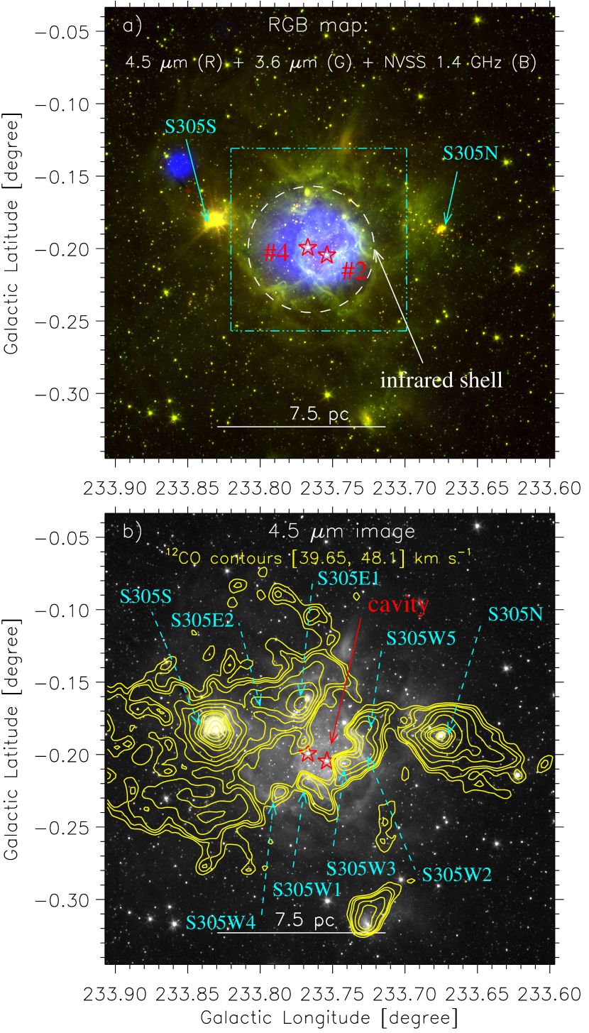
Figure 1.— a) Three-color composite image (red, Spitzer 4.5 $\mu$m; green, Spitzer 3.6 $\mu$m; blue, NVSS 1.4 GHz) of the region around S305 (selected area $\sim$18^′.7 $\times$ 18^′.7 centered at l = 233$\arcdeg$.75; b = $-$0$\arcdeg$.19). An extended shell-like feature is highlighted by a big broken circle (in white). A dotted-dashed box (in cyan) encompasses the area shown in Figure 2a. b) Overlay of the FUGIN ¹²CO(J =1$-$0) gas on the Spitzer 4.5 $\mu$m image. The ¹²CO integrated velocity range is from 39.65 to 48.1 km s^-1 (1$\sigma$ $\sim$2.2 K km s^-1). The ¹²CO contours (in yellow) are 19.5, 22.5, 25, 32, 40, 50, 63, 70, 75, 85, 95, and 105 K km s^-1. A cavity area is indicated by an arrow (in red). Several SCUBA2 850 $\mu$m continuum clumps (from Sreenilayam et al., 2014) are labeled in the figure (see Figure 5 in their paper). In each panel, the positions of previously known two massive O9.5V (#2) and O8.5V (#4) stars are marked by stars, and a scale bar referring to 7.5 pc (at a distance of 3.7 kpc) is shown.

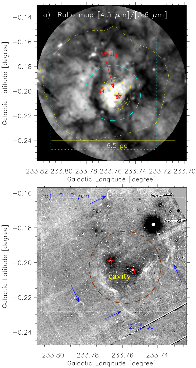
Figure 2.— a) Overlay of the NVSS radio continuum contours (in yellow) on the Spitzer ratio map of 4.5 $\mu$m/3.6 $\mu$m emission of an area highlighted by a dotted-dashed box in Figure 1a. The NVSS contours are shown with the levels of 2.3, 100, 110, 120, 130, 135, and 140 mJy beam^-1. A dotted box (in cyan) encompasses the area shown in Figure 2b. b) Continuum-subtracted H₂ image at 2.12 $\mu$m (in gray-scale) of an area highlighted by a dotted box in Figure 2a. Arrows and a dashed circle indicate the detections of the H₂ emission. A dotted-dashed box (in yellow) encompasses the area shown in Figures 3a, 3b, 3c, and 3d. The ratio map and the H₂ image are smoothened using a Gaussian function with radius of four pixels. In each panel, the positions of previously known two massive O9.5V (#2) and O8.5V (#4) stars are marked by stars, and a dashed circle highlights the immediate surroundings of massive stars (see text for more details).

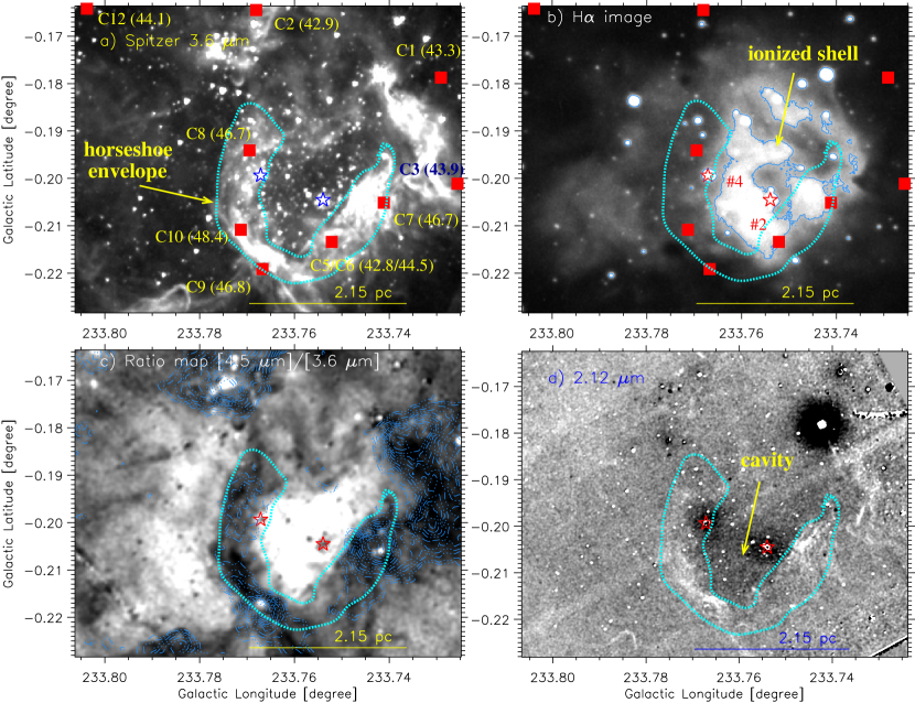
Figure 3.— a) Gray-scale Spitzer 3.6 $\mu$m image of an area highlighted by a broken box in Figure 2b. The positions of observed molecular clumps (from Azimlu & Fich, 2011) are highlighted by filled squares, which are also labeled in the figure. The radial velocity of the molecular gas (in km s^-1) toward each clump (from Azimlu & Fich, 2011) is also indicated in the figure. b) Gray-scale H$\alpha$ image of the same area as shown in in Figure 3a. A solid contour (in dodger blue) shows an ionized shell traced in the H$\alpha$ image. Filled squares are the same as shown in Figure 3a. c) The panel shows the Spitzer ratio map of 4.5 $\mu$m/3.6 $\mu$m emission (see also Figure 2a). The ratio map is also overlaid with the contours (in dodger blue) of the JCMT SCUBA2 continuum emission at 850 $\mu$m (see also Figure 5b). d) Continuum-subtracted H₂ image at 2.12 $\mu$m (in gray-scale; see also Figure 2b). An arrow shows the gas and dust deficient region, which is referred to as cavity. In each panel, the positions of previously known two massive O9.5V (#2) and O8.5V (#4) stars are marked by stars, and a scale bar referring to 2.15 pc (at a distance of 3.7 kpc) is marked. In all panels, a dotted curve (in cyan) indicates walls of a cavity.

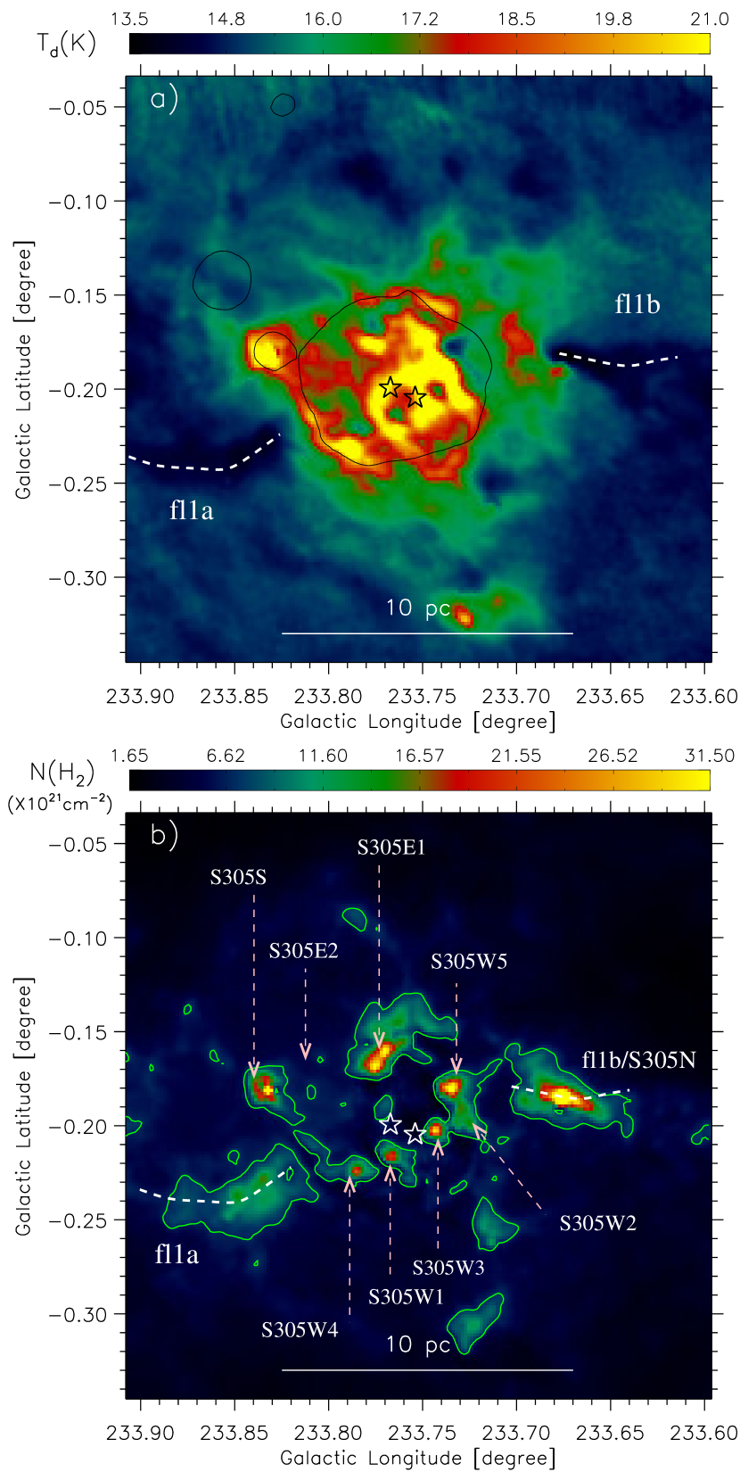
Figure 4.— a) Overlay of the NVSS radio continuum contour (at 2.3 mJy beam^-1) on the Herschel temperature map of the selected region around S305. b) Herschel column density ($N(\mathrm{H}_{2})$) map. The $N(\mathrm{H}_{2})$ contour (in green) is also shown with a level of 6.85 $\times$ 10²¹ cm^-2. Several SCUBA2 850 $\mu$m continuum clumps (from Sreenilayam et al., 2014) are labeled in the figure (see also Figure 1b). In both panels, stars show the positions of two massive O-type stars, and two broken curves (in white) highlight both ends of an elongated filament (i.e., fl1a and fl1b). In each panel, the scale bar referring to 10 pc (at a distance of 3.7 kpc) is shown.

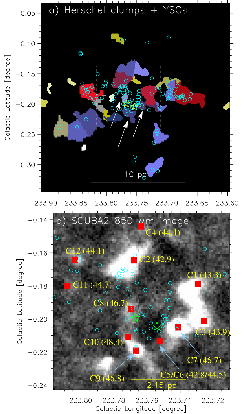
Figure 5.— a) Distribution of YSOs (see cyan circles) against the boundaries of the Herschel clumps. Different colors are utilized to distinguish the clumps. All these results are taken from Pandey et al. (2020) (see Figures 12 and 13 in their paper). Arrows indicate the locations of the Herschel clumps seen toward the horseshoe envelope. b) JCMT SCUBA2 continuum emission map at 850 $\mu$m of an area highlighted by a dashed box in Figure 5a. The positions of 12 molecular clumps (from Azimlu & Fich, 2011) are highlighted by filled squares, which are also labeled in the figure. Circles show the position of YSOs. The radial velocity of the molecular gas toward each clump (from Azimlu & Fich, 2011) is also indicated in the figure (see also Figure 3a).

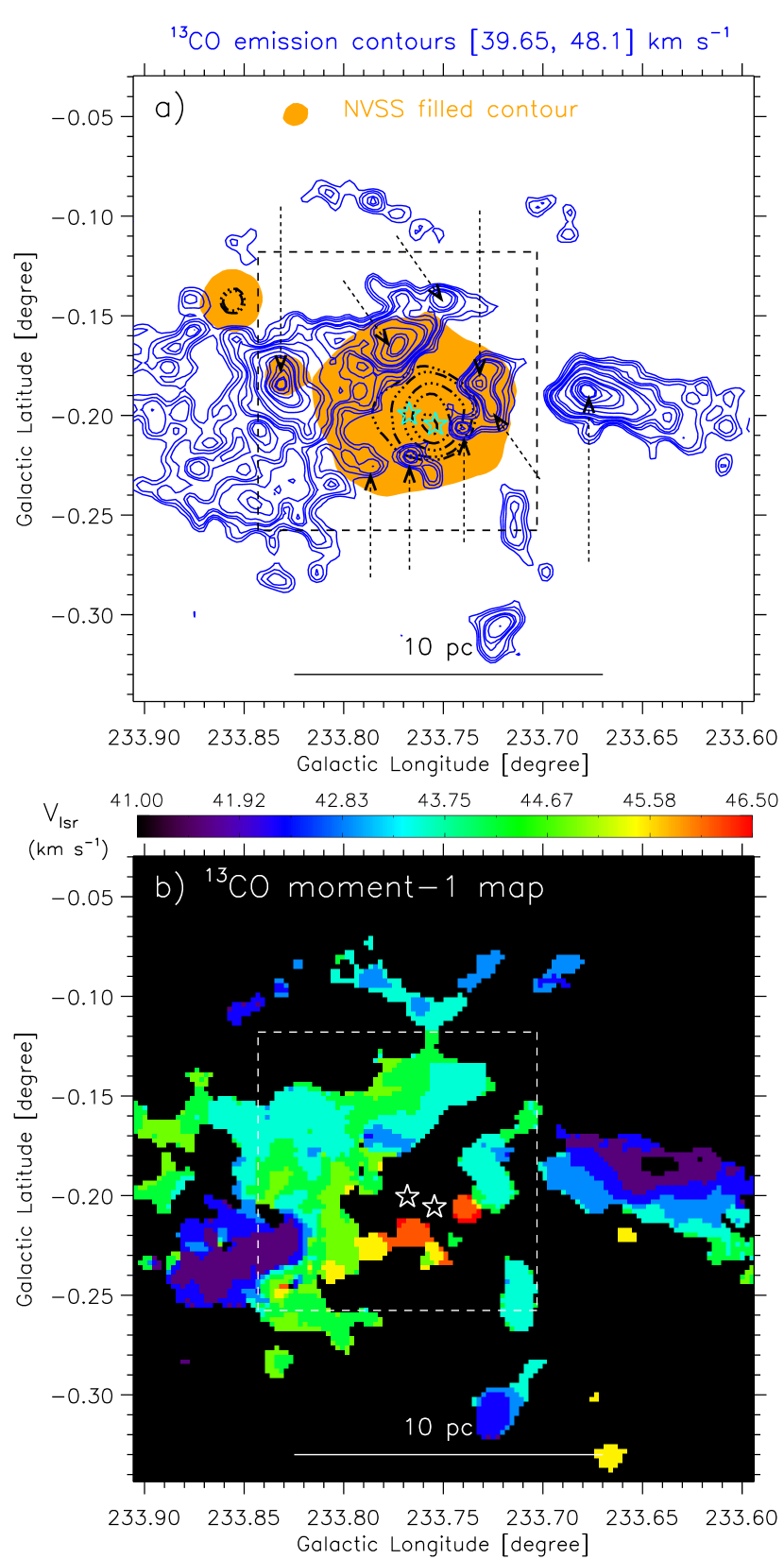
Figure 6.— a) Overlay of the FUGIN ¹³CO(J=1$-$0) emission on the filled NVSS contour map (at 2.3 mJy beam^-1; in orange). The ¹³CO integrated velocity range is from 39.65 to 48.1 km s^-1 (1$\sigma$ $\sim$0.85 K km s^-1). The ¹³CO contours (in blue) are 3.6, 4.3, 5, 6.2, 6.7, 7.5, 9, 10, 13, 16, 17.3, 20, 22, 24, and 24.6 K km s^-1. We also show in broken-line black contours the 50, 60, 85, 110, and 135 mJy beam^-1 flux levels at 1.4 GHz. Several molecular condensations surrounding massive stars are highlighted by black arrows (see also Figure 1b). b) Intensity-weighted mean velocity (moment-1) map of ¹³CO. In each panel, stars show the positions of two massive O-type stars, and the scale bar referring to 10 pc (at a distance of 3.7 kpc) is displayed.

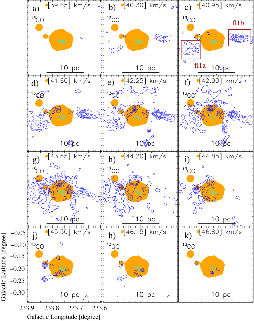
Figure 7.— Velocity channel contours of ¹³CO emission. The velocity of molecular emission is marked in each panel (in km s^-1). The contour levels of ¹³CO are presented with the levels of 1, 2, 3, 4, 5.5, and 6.5 K km s^-1. In panel “c”, solid boxes highlight both ends of the filament (i.e., fl1a and fl1b) traced in the Herschel column density map. In each panel, the NVSS filled contour is shown in the background with a level of 2.3 mJy beam^-1 (see also Figure 6a). In all panels, stars show the positions of two massive O-type stars.

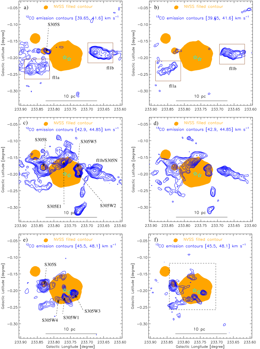
Figure 8.— Left panels (i.e., a, c, e): Velocity channel contours of ¹²CO emission at different velocity intervals. In panel “a”, the contours of ¹²CO are 5.5, 7, 8, 9.5, 10.5, 14, 18, 22, 24, and 26 K km s^-1. In panel “c”, the contours of ¹²CO are 13.8, 15, 17, 18.5, 21.5, 23.5, 26, 29, 33, 38, 40, 43, and 49 K km s^-1. In panel “e”, the contours of ¹²CO are 8.5, 11, 13, 14.2, 18, 21, 25, 29, 36, 40, and 45 K km s^-1. Right panels (i.e., b, d, f): Velocity channel contours of ¹³CO emission at different velocity intervals. In panel “b”, the contours of ¹³CO are 1.6, 1.95, 2.6, 3, 4, 5, 6, and 6.6 K km s^-1. In panel “d”, the contours of ¹³CO are 3, 3.5, 4.3, 5.5, 6.8, 8.3, 10, 12, 12.8, and 14 K km s^-1. In panel “f”, the contours of ¹³CO are 1.8, 2.4, 3.2, 4, 4.8, 6, 7.3, 8.8, and 9.8 K km s^-1. In panel “f”, a dashed box (in black) encompasses the area shown in Figures 9a, 9b, and 9c. In each panel, the NVSS filled contour is shown in the background with a level of 2.3 mJy beam^-1 (see also Figure 6a). In panels “a” and “b”, solid boxes represent both ends of the filament (i.e., fl1a and fl1b). In all panels, stars show the positions of two massive O-type stars. The velocity interval of molecular emission (in km s^-1) is indicated in each panel.

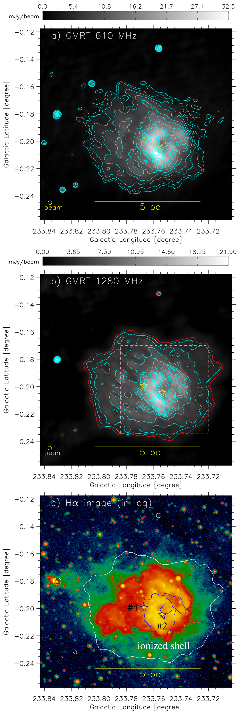
Figure 9.— a) Overlay of the GMRT 610 MHz continuum contours on the 610 MHz gray scale map (resolution $\sim$ 10^′′ $\times$ 10^′′; see dashed box in Figure 8f). The GMRT 610 MHz continuum contour levels (in cyan) are 2.2, 3, 4.5, 6.5, 9.5, 12, 15, 16.5, 18, 20, 21.3, 24, 25.5, 27, 29, and 31 mJy beam^-1 (with $\sigma\sim 0.46$ mJy beam^-1). b) Overlay of the GMRT 1280 MHz continuum contours on the 1280 MHz gray scale map (resolution $\sim$ 10^′′ $\times$ 10^′′). The GMRT 1280 MHz continuum contour levels (in cyan) are 3, 4, 6, 8, 9, 10, 11, 12, 13, 14, 15, 16, 17, and 18 mJy beam^-1 (with $\sigma$ $\sim$0.74 mJy beam^-1). The GMRT 1280 MHz continuum level at 2.5 mJy beam^-1 is shown with a red contour. A pink dashed box encompasses the area shown in Figures 11a, 11b, 11c, and 11d. c) Overlay of the GMRT 1280 MHz continuum contours (at 2.5 and 10.5 mJy beam^-1) on the H$\alpha$ image. In all panels, stars show the positions of two massive O-type stars (see also Figure 1a).

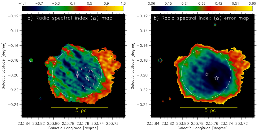
Figure 10.— a) GMRT spectral index map (resolution $\sim$10^′′) of S305 generated for pixels above 3$\sigma$ level in the 610 and 1280 MHz bands. The GMRT 1280 MHz continuum emission is also shown by a dotted-dashed contour at 10.5 mJy beam^-1. Regions with non-thermal $\alpha$ are greenish-blue, while regions consistent with thermal emission are red-yellow. b) GMRT spectral index error map of S305. In both panels, stars show the positions of two massive O-type stars (see also Figure 1a), and a big circle (in white) highlights the central region of S305.

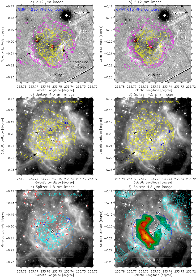
Figure 11.— a) Overlay of the GMRT 1280 MHz continuum contours (in magenta and yellow) on the continuum subtracted H₂ image at 2.12 $\mu$m (see a dashed box in Figure 9b and also Figure 2b). The contour levels in magenta are 7.5, 8, 9, and 9.8 mJy beam^-1, while the yellow contours are 10.5, 11, 12, 13, 14, 15, 16, 17, 18, and 18.5 mJy beam^-1. b) Overlay of the GMRT 610 MHz continuum contours (in magenta and yellow) on the continuum subtracted H₂ image at 2.12 $\mu$m. The magenta contour levels are 10.5, 11.5, 13.5, 14.5, and 15.5 mJy beam^-1, while the yellow ones are 16.5, 18, 20.5, 23, 25, 26, 29, and 31 mJy beam^-1. c) Overlay of the GMRT 1280 MHz continuum contours (in yellow) on the Spitzer 4.5 $\mu$m image (see Figure 11a). d) Overlay of the GMRT 610 MHz continuum contours (in yellow) on the Spitzer 4.5 $\mu$m image (see Figure 11b). e) The panel is the same as in Figure 11c, but it is overlaid with the positions of YSOs (see small red circles; from Pandey et al., 2020). The GMRT 1280 MHz continuum contours (in cyan) are shown with the levels of 11, 12, 13, 14, 15, 16, 17, 18, and 18.5 mJy beam^-1. f) The panel is the same as in Figure 11e, but it is overlaid the $N(\mathrm{H}_{2})$ contours (in cyan). The $N(\mathrm{H}_{2})$ contours (in cyan) are presented with the levels of (7.0, 8.0, 9.0, 10.0, 11.0, 13.0, 15.0, 17.0, 19.0, 21.0, 26.0, and 28.5) $\times$ 10²¹ cm^-2 (see also Figure 4b). The GMRT 1280 MHz continuum emission is displayed by filled contours. In panels “c” and “d”, four selected radio peaks are labeled (“A–D”). In panels “c” and “e”, the position of a point-like source toward each radio peak is shown by an upside down triangle. In the last two panels, a big circle (extension $\sim$2.15 pc) highlights a ring-like radio morphology around a massive O9.5V (#2) star. In all panels, stars show the positions of two massive O-type stars (see also Figure 1a).

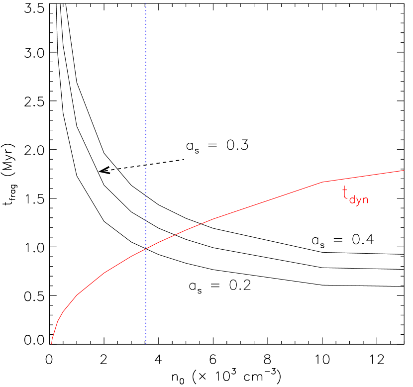
Figure 12.— Dynamical time (red curve) and fragmentation timescale (black curves) as a function of the initial density of the ambient medium. The fragmentation timescale is computed for three values of sound speeds of neutral gas ($a_{s}$ = 0.2 , 0.3, and 0.4 km s^-1). A dotted vertical line is shown at density of 3530 cm^-3.

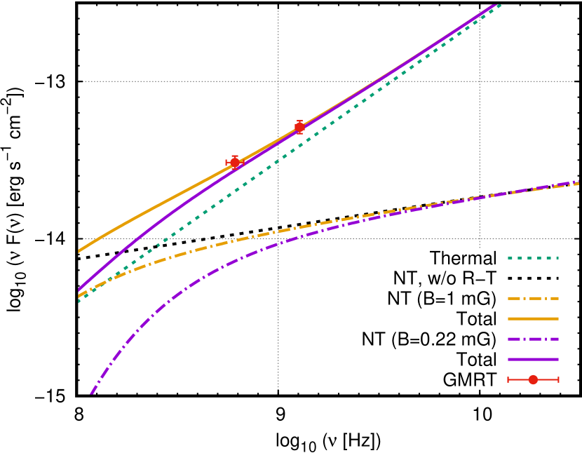
Figure 13.— Observed spectral energy distribution of S305 at radio frequencies. We fit the spectrum as a composite spectrum of a thermal component from the ionized gas plus a non-thermal (NT) component from locally-accelerated relativistic electrons. We show the emission model for extreme scenarios of a high magnetic field ($B\approx 1$ mG) and a low magnetic field ($B\approx 0.22$ mG). For comparison, we also show the synchrotron component without accounting for the Razin-Tsytovich effect (dotted black line; see Sect. 4.2 for details).

References

- Azimlu & Fich (2011) Azimlu, M., Fich, M. 2011, AJ, 141. 43-49
- Balser et al. (2011) Balser, D. S., Rood, R. T., Bania, T. M., and Anderson, L. D. 2011, ApJ, 738, 27
- Baug et al. (2015) Baug, T., Ojha, D. K., Dewangan, L. K., et al. 2015, MNRAS, 454, 4335
- Benjamin et al. (2003) Benjamin, R. A.,Churchwell, E., Babler, B. L., et al. 2003, PASP, 115, 953
- Bertoldi (1989) Bertoldi, F. 1989, ApJ, 346, 735
- Bihr et al. (2016) Bihr, S. , Johnston, K. G., Beuther, H., et al. 2016, A&A, 588, 97
- Binder et al. (2018) Binder, B. A. & Povich, M. S. 2018, ApJ, 864, 136
- Bisbas et al. (2009) Bisbas, T. G., Wünsch, R., Whitworth, A. P., & Hubber, D. A. 2009, A&A, 497, 649
- Brand et al. (2011) Brand, J., Massi, F., Zavagno, A., Deharveng, L., & Lefloch, B. 2011, A&A, 527, 62
- Chini & Wink (1984) Chini, R., and Wink, J. E. 1984, A&A, 139, L5
- Condon et al. (1998) Condon, J. J., Cotton, W. D., Greisen, E. W., et al. 1998, AJ, 115, 1693
- Dale et al. (2007) Dale, J. E., Clark, P. C., & Bonnell, I. A. 2007, MNRAS, 377, 535
- Dale et al. (2015) Dale, J. E., Haworth, T. J., Bressert, E. 2015, MNRAS, 450, 1199
- Deharveng et al. (2003) Deharveng, L., Lefloch, B., Zavagno, A., et al 2003, A&A, 408, 25L
- Deharveng et al. (2005) Deharveng, L., Zavagno, A., & Caplan, J. 2005, A&A, 433, 565
- Deharveng et al. (2006) Deharvengm L., Leflochm B., Massim F., et al. 2006, A&A, 458, 191
- Deharveng et al. (2008) Deharveng, L., Lefloch, B., Kurtz, S., et al. 2008, A&A, 482, 585
- Deharveng et al. (2010) Deharveng, L., Schuller, F., Anderson, L. D., et al. 2010, A&A, 523, 6
- Dewangan & Anandarao (2011) Dewangan, L. K., & Anandarao, B. G. 2011, MNRAS, 414, 1526
- Dewangan et al. (2012) Dewangan, L. K., Ojha, D. K., Anandarao, B. G., Ghosh, S. K., & Chakraborti, S. 2012, ApJ, 756, 151
- Dewangan et al. (2015) Dewangan, L. K., Ojha, D. K., Grave, J. M. C., & Mallick, K. K. 2015, MNRAS, 446, 2640
- Dewangan et al. (2016) Dewangan, L. K., Ojha, D. K., Luna, A., et al. 2016, ApJ, 819, 66
- Dewangan et al. (2017) Dewangan, L. K., Ojha, D. K., Zinchenko, I., Janardhan, P., & Luna, A. 2017, ApJ, 834, 22
- Dougherty et al. (2003) Dougherty, S. M., Pittard, J. M., Kasian, L., Coker, R. F., Williams, P. M., & Lloyd, H. M. 2003, A&A, 409, 217
- Dyson & Williams (1980) Dyson, J. E., & Williams, D. A. 1980, Physics of the interstellar medium, New York, Halsted Press, 204 p
- Elmegreen & Lada (1977) Elmegreen, B. G., & Lada, C. J. 1977, ApJ, 214, 725
- Elmegreen (1998) Elmegreen, B. G. 1998, in ASP Conf. Ser. 148, Origins, ed. C. E. Woodward, J. M. Shull, & H. A. Thronson, Jr. (San Francisco, CA: ASP), 150
- Evans et al. (2009) Evans, N. J., II, Dunham, M. M., Jrgensen, J. K., et al. 2009, ApJS, 181, 321
- Fransson & Björnsson (1998) Fransson, C., & Björnsson, C. 1998, ApJ, 509, 861
- Freeney-Johansson et al. (2019) Freeney-Johansson, A., Purser, S. J. D., Ray, T. P., et al. 2019, ApJL, 885, 7
- Hou & Han (2014) Hou, L. G. & Han, J. L. 2014, A&A 569, 125
- Inoue (2001) Inoue, A. K. 2001, AJ, 122, 1788
- Inoue et al. (2001) Inoue, A. K., Hirashita, H., & Kamaya, H. 2001, ApJ, 555, 613
- Kwan (1997) Kwan, J. 1997, ApJ, 489, 284
- Lefloch & Lazareff (1994) Lefloch, B., & Lazareff, B. 1994, A&A, 289, 559
- Longair (1992) Longair, M. S. 1992, High energy astrophysics. Vol.1: Particles, photons and their detection, 436
- Mallick et al. (2012) Mallick, K. K., Ojha, D. K., Samal, M. R., et al. 2012, ApJ, 759, 48
- Mallick et al. (2013) Mallick, K. K., Kumar, M. S. N., Ojha, D. K., et al. 2013, ApJ, 779, 113
- Marcote et al. (2015) Marcote, B., Ribó, M., Paredes, J. M., & Ishwara-Chandra, C. H. 2015, MNRAS, 451, 59
- Marsh et al. (2015) Marsh, K. A., Whitworth, A. P., & Lomax, O. 2015, MNRAS, 454, 4282
- Marsh et al. (2017) Marsh, K. A., Whitworth, A. P., Lomax, O., et al. 2017, MNRAS, 471, 2730
- Matsakis et al. (1976) Matsakis, D. N., Evans, N. J., II, Sato, T., & Zuckerman, B. 1976, AJ, 81, 172
- Melrose (1980) Melrose, D. B. 1980, Plasma astrohysics. Nonthermal processes in diffuse magnetized plasmas - Vol.1: The emission, absorption and transfer of waves in plasmas; Vol.2: Astrophysical applications
- Molinari et al. (2010a) Molinari, S., Swinyard, B., Bally, J., et al., 2010a, A&A, 518, L100
- Molinari et al. (2010b) Molinari, S., Swinyard, B., Bally, J., et al., 2010b, PASP, 122, 314
- Nandakumar et al. (2016) Nandakumar, G., Veena, V. S., Vig, S., et al. 2016, AJ, 152, 146
- Navarete et al. (2015) Navarete, F., Damineli, A., Barbosa, C. L., & Blum, R. D. 2015, MNRAS, 450, 4364
- Padovani et al. (2019) Padovani, M., Marcowith, A., Sánchez-Monge, Á., Meng, F., & Schilke, P. 2019, A&A, 630, A72
- Panagia (1973) Panagia, N. 1973, AJ, 78, 929
- Pandey et al. (2020) Pandey, R., Sharma, Saurabh, Panwar, N., Dewangan, L. K., Ojha, D. K. et al.; 2020, ApJ; astroph ref: arXiv:2001.04722
- Parker et al. (2005) Parker, Q. A., Phillipps, S., Pierce, M. J., et al. 2005, MNRAS, 362, 689
- Prajapati et al. (2019) Prajapati, P., Tej, A., del Palacio, S., et al. 2019, ApJL, 884, 49
- Russeil et al. (1995) Russeil, D., Georgelin, Y. M., Georgelin, Y. P., Le Coarer, E., and Marcelin, M. 1995, A&AS, 114, 557
- Rybicki & Lightman (1979) Rybicki, G. B., and Lightman, A. P. 1979, Radiative processes in astrophysics
- Sreenilayam et al. (2014) Sreenilayam, G., Fich, M., Ade, P., et al. 2014, AJ, 147, 3
- Tan et al. (2014) Tan, J. C., Beltrán, M. T., Caselli, P., et al. 2014, in Protostars and Planets VI, ed. H. Beuther et al. (Tucson, AZ: Univ. Arizona Press), 149
- Veena et al. (2016) Veena, V. S., Vig, S., Tej, A., et al. 2016, MNRAS, 456, 2425
- Vogt & Moffat (1975) Vogt, N., and Moffat, A. F. J. 1975, A&A, 45, 405
- Umemoto et al. (2017) Umemoto, T., Minamidani, T., Kuno, N., et al. 2017 PASJ, 69, 78
- Whitney et al. (2011) Whitney, B., Benjamin, R., Meade, M., et al. 2011, BAAS, 43, 241.16
- Whitworth et al. (1994) Whitworth, A. P., Bhattal, A. S., Chapman, S. J., Disney, M. J., & Turner, J. A. 1994, MNRAS, 268, 291
- Williams et al. (1994) Williams, J. P., de Geus, E. J., & Blitz, L. 1994, ApJ, 428, 693
- Xu et al. (2017) Xu, Jin-Long, Xu, Y., Yu, N., et al. 2017, ApJ, 849, 140
- Zavagno et al. (2006) Zavagno, A., Deharveng, L., Comeron, F., et al. 2006, A&A, 446, 171
- Zavagno et al. (2007) Zavagno, A., Pomares, M., Deharveng, L., et al. 2007, A&A, 472, 835
- Zavagno et al. (2010) Zavagno, A., Russeil, D., Motte, F., et al. 2010, A&A, 518, L81
- Zinnecker & Yorke (2007) Zinnecker, H., & Yorke, H. W. 2007, ARA&A, 45, 481