mFI-PSO: A Flexible and Effective Method
in Adversarial Image Generation for
Deep Neural Networks

Abstract

Deep neural networks (DNNs) have achieved great success in image classification, but can be very vulnerable to adversarial attacks with small perturbations to images. To improve adversarial image generation for DNNs, we develop a novel method, called mFI-PSO, which utilizes a Manifold-based First-order Influence measure for vulnerable image and pixel selection and the Particle Swarm Optimization for various objective functions. Our mFI-PSO can thus effectively design adversarial images with flexible, customized options on the number of perturbed pixels, the misclassification probability, and the targeted incorrect class. Experiments demonstrate the flexibility and effectiveness of our mFI-PSO in adversarial attacks and its appealing advantages over some popular methods.

I Introduction

Deep neural networks (DNNs) have exhibited exceptional performance in image classification [1, 2, 3] and thus are widely used in various real-world applications including face recognition [4], self-driving cars [5], biomedical image processing [6], among many others [7]. Despite these successes, DNN classifiers can be easily attacked by adversarial examples with perturbations imperceptible to human vision [8, 9, 10]. This motivates the hot research in adversarial attacks and defenses of DNNs [11, 12].

Existing adversarial attacks can be categorized into white-box, gray-box, and black-box attacks. Adversaries in white-box attacks have the full information of their targeted DNN model, whereas their knowledge is limited to model structure in gray-box attacks and only to model’s input and output in black-box attacks. For instance, popular algorithms for white-box attacks include the fast gradient sign method (FGSM) [9], the projected gradient descent (PGD) method [13], the Carlini and Wagner (CW) attack [14], the Jacobian-based saliency map attack (JSMA) [15], DeepFool [16], among many others [8, 17].

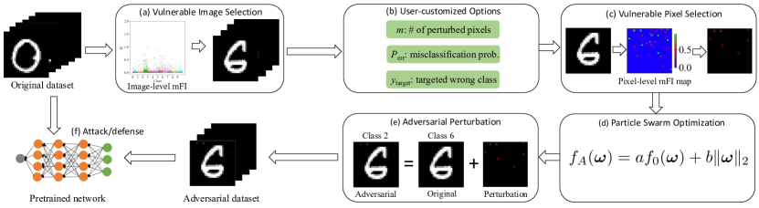
Figure 1: Flowchart of our mFI-PSO method.

In this paper, we propose a simple yet efficient method for white-box adversarial image generation for DNN classifiers. For generating an adversarial example of a given image, our method provides user-customized options on the number of perturbed pixels, misclassification probability, and targeted incorrect class. To the best of our knowledge, this is the first approach rendering all the three desirable options.

The freedom to specify the number of perturbed pixels allows users to conduct attacks at various pixel levels such as one-pixel [10], few-pixel [15], and all-pixel [18] attacks. In particular, we adopt a recent manifold-based first-order influence (mFI) measure [19] to efficiently locate the most vulnerable pixels to increase the attack success rate. Besides, to generate a high-quality adversarial image set, our method also utilizes the mFI measure to identify vulnerable images in a given dataset. In contrast with traditional Euclidean-space based measures such as Jacobian norm [20] and Cook’s local influence measure [21], the mFI measure captures the “intrinsic” change of the perturbed objective function [22, 23] and shows better performance in detecting vulnerable images and pixels.

Our method allows users to specify the misclassification probability for a targeted or nontargeted attack. The prespecified misclassification probability is rarely seen in existing approaches, which produce an adversarial example either near the model’s decision boundary [16, 24] or with unclear confidence [25]. For instance, the CW attack [14] uses a $\kappa$ parameter to control the confidence of an adversarial example, but the parameter is not the misclassification probability that is more user-friendly. In addition, the CW method does not provide the option to control the number of perturbed pixels.

Moreover, we tailor different loss functions accordingly to the above three desirable options and their combinations, and apply the particle swarm optimization (PSO) [26] to obtain the optimal perturbation. The PSO is a widely-used gradient-free method that is preferred over gradient-based methods in solving nonconvex or nondifferentiable problems [27, 28], and thus provides us much freedom to design various loss functions to meet users’ needs.

Our proposed method is named as mFI-PSO, based on its combination nature of the mFI measure and the PSO algorithm. Figure 1 illustrates the flowchart of our method.

We notice that two recent papers [29, 30] also applied PSO to craft adversarial images. However, we have intrinsic distinctions. First, the two papers focus on black-box attacks, but ours is white-box. Article [29] only studied all-pixel attacks; although article [30] considered few-pixel attacks but searched in random chunks to locate the vulnerable pixels, we use the mFI measure to directly discover those pixels. Moreover, targeted attacks are not considered in [30], and both papers cannot prespecify a misclassification probability for the generated adversarial example. Our mFI-PSO method is able to design arbitrary-pixel-level, confidence-specified, and/or targeted/nontargeted attacks.

Our contributions are summarized as follows:

• We propose a novel white-box method for adversarial image generation for DNN classifiers. It provides users with multiple options on pixel levels, confidence levels, and targeted classes for adversarial attacks.

• We innovatively adopt a mFI measure based on an “intrinsic” perturbation manifold to efficiently identify vulnerable images and pixels for adversarial perturbations.

• We design various different loss functions adaptive to user-customized specifications and apply the PSO, a gradient-free optimization, to obtain optimal perturbations.

• We demonstrate the flexibility and effectiveness of our mFI-PSO method in adversarial attacks via experiments on benchmark datasets and show its winning advantages over some commonly-used methods.

The Python code to implement the proposed mFI-PSO is available at https://github.com/BruceResearch/mFI-PSO.

II Method

II-A Manifold-based Influence Measure

Given an input image $\boldsymbol{x}$ and a DNN classifier $N$ with parameters $\boldsymbol{\theta}$, the prediction probability for class $y\in\{1,\dots,K\}$ is denoted by $P(y|\boldsymbol{x},\boldsymbol{\theta})=N_{\boldsymbol{\theta}}(y,\boldsymbol{x})$. Let $\boldsymbol{\omega}=(\omega_{1},\dots,\omega_{m})^{T}$ be a perturbation vector in an open set $\Omega\subseteq\mathbb{R}^{m}$, which can be imposed on any subvector of $(\boldsymbol{x}^{T},\boldsymbol{\theta}^{T})^{T}$. Let the prediction probability under perturbation $\boldsymbol{\omega}$ be $P(y|\boldsymbol{x},\boldsymbol{\theta},\boldsymbol{\omega})$ with $P(y|\boldsymbol{x},\boldsymbol{\theta},\boldsymbol{\omega}_{0})=P(y|\boldsymbol{x},\boldsymbol{\theta})$ and $\boldsymbol{\omega}_{0}\in\Omega$.

For sensitivity analysis of DNNs, article [19] recently has proposed a mFI measure to delineate the intrinsic perturbed change of the objective function on a Riemannian manifold. In contrast with traditional Euclidean-space based measures such as Jacobian norm [20] and Cook’s local influence measure [21], this perturbation-manifold based measure enjoys the desirable invariance property under diffeomorphic (e.g., scaling) reparameterizations of perturbations and has better numerical performance in detecting vulnerable images and pixels.

Let $f(\boldsymbol{\omega})$ be an objective function of interest, for example, the cross-entropy $f(\boldsymbol{\omega})=-\log P(y=y_{\text{true}}|\boldsymbol{x},\boldsymbol{\theta},\boldsymbol{\omega})$. The mFI measure at $\boldsymbol{\omega}=\boldsymbol{\omega}_{0}$ is defined by

$$\text{mFI}_{\boldsymbol{\omega}}(\boldsymbol{\omega}_{0})=[\partial_{\boldsymbol{\omega}}f(\boldsymbol{\omega}_{0})]\mathbf{G}^{\dagger}_{\boldsymbol{\omega}}(\boldsymbol{\omega}_{0})[\partial_{\boldsymbol{\omega}}f(\boldsymbol{\omega}_{0})]^{T},$$ (1)

where $\partial_{\boldsymbol{\omega}}=(\partial/\partial{\omega}_{1},\dots,\partial/\partial{\omega}_{m})$, $\mathbf{G}_{\boldsymbol{\omega}}(\boldsymbol{\omega})=\sum_{y=1}^{K}\partial_{\boldsymbol{\omega}}^{T}\ell(\boldsymbol{\omega}|y,\boldsymbol{x},\boldsymbol{\theta})\partial_{\boldsymbol{\omega}}\ell(\boldsymbol{\omega}|y,\boldsymbol{x},\boldsymbol{\theta})P(y|\boldsymbol{x},\boldsymbol{\theta},\boldsymbol{\omega})$ with $\ell(\boldsymbol{\omega}|y,\boldsymbol{x},\boldsymbol{\theta})=\log P(y|\boldsymbol{x},\boldsymbol{\theta},\boldsymbol{\omega})$, and $\mathbf{G}^{\dagger}_{\boldsymbol{\omega}}(\boldsymbol{\omega}_{0})$ is the pseudoinverse of $\mathbf{G}_{\boldsymbol{\omega}}(\boldsymbol{\omega}_{0})$. A larger value of $\text{mFI}_{\boldsymbol{\omega}}(\boldsymbol{\omega}_{0})$ indicates that the DNN model is more sensitive in $f(\boldsymbol{\omega})$ to local perturbation $\boldsymbol{\omega}$ around $\boldsymbol{\omega}_{0}$.

In (1), we can see that $\text{mFI}_{\boldsymbol{\omega}}(\boldsymbol{\omega}_{0})$ is an extension of the squared Jacobian norm $\|\mathbf{J}_{\boldsymbol{\omega}}(\boldsymbol{\omega}_{0})\|_{F}^{2}=\partial_{\boldsymbol{\omega}}f(\boldsymbol{\omega}_{0})[\partial_{\boldsymbol{\omega}}f(\boldsymbol{\omega}_{0})]^{T}$ that is corrected with $\mathbf{G}^{\dagger}_{\boldsymbol{\omega}}(\boldsymbol{\omega}_{0})$. When $\mathbf{G}_{\boldsymbol{\omega}}(\boldsymbol{\omega}_{0})=\mathbf{I}$, $\text{mFI}_{\boldsymbol{\omega}}(\boldsymbol{\omega}_{0})$ reduces to $\|\mathbf{J}_{\boldsymbol{\omega}}(\boldsymbol{\omega}_{0})\|_{F}^{2}$. Note that $\mathbf{G}_{\boldsymbol{\omega}}(\boldsymbol{\omega})$ is the metric tensor of the pseudo-Riemannian manifold $\mathcal{M}=\{P(y|\boldsymbol{x},\boldsymbol{\theta},\boldsymbol{\omega}):\boldsymbol{\omega}\in\Omega\}$. If $\mathbf{G}_{\boldsymbol{\omega}}(\boldsymbol{\omega})$ is positive definite, then it can define an inner product on $T_{\boldsymbol{\omega}}=span(\{\partial\ell(\boldsymbol{\omega}|y,\boldsymbol{x},\boldsymbol{\theta})/\partial\omega_{i}\}_{i=1}^{m})$ which is the tangent space of $\mathcal{M}$ at point $\boldsymbol{\omega}$, and thus can measure the distance of two points on $\mathcal{M}$. However, $\mathbf{G}_{\boldsymbol{\omega}}(\boldsymbol{\omega})$ is a singular matrix when the dimension of $\boldsymbol{\omega}$ is larger than the number of classes, i.e., $m>K$. The singularity of $\mathbf{G}_{\boldsymbol{\omega}}(\boldsymbol{\omega})$ indicates that $\partial\ell/\partial\omega_{1},\dots,\partial\ell/\partial\omega_{m}$, which span $T_{\boldsymbol{\omega}}$, are linearly dependent and thus some components of $\boldsymbol{\omega}$ are redundant. Therefore, $\boldsymbol{\omega}$ is transformed to a low-dimensional vector $\boldsymbol{\nu}$ by $\boldsymbol{\nu}=\mathbf{\Lambda}_{0}^{1/2}\mathbf{U}_{0}^{T}\boldsymbol{\omega}$, where $\mathbf{U}_{0}\in\mathbb{R}^{m\times r_{0}}$, with $r_{0}=\text{rank}(\mathbf{G}_{\boldsymbol{\omega}}(\boldsymbol{\omega}_{0}))$, and the diagonal matrix $\mathbf{\Lambda}_{0}$ form the compact singular value decomposition $\mathbf{G}_{\boldsymbol{\omega}}(\boldsymbol{\omega}_{0})=\mathbf{U}_{0}\mathbf{\Lambda}_{0}\mathbf{U}_{0}^{T}$. Then, $\mathcal{M}_{\boldsymbol{\nu}_{0}}=\{P(y|\boldsymbol{x},\boldsymbol{\theta},\boldsymbol{\nu}):\boldsymbol{\nu}\in B_{\boldsymbol{\nu}_{0}}\}$ is a Riemannian manifold with a positive-definite metric tensor $\mathbf{G}_{\boldsymbol{\nu}}(\boldsymbol{\nu})$ in some open ball $B_{\boldsymbol{\nu}_{0}}$ centered at $\boldsymbol{\nu}_{0}=\mathbf{\Lambda}_{0}^{1/2}\mathbf{U}_{0}^{T}\boldsymbol{\omega}_{0}$, and moreover, $\mathbf{G}_{\boldsymbol{\nu}}(\boldsymbol{\nu}_{0})=\mathbf{I}$. This indicates that $\partial\ell/\partial\nu_{1},\dots,\partial\ell/\partial\nu_{r_{0}}$ are a basis of the tangent space, $T_{\boldsymbol{\nu}}$, of $\mathcal{M}_{\boldsymbol{\nu}_{0}}$ at $\boldsymbol{\nu}$, and are an orthonormal basis of $T_{\boldsymbol{\nu}}$ at $\boldsymbol{\nu}=\boldsymbol{\nu}_{0}$. We can thus view $\boldsymbol{\nu}$ as the intrinsic representation of perturbation $\boldsymbol{\omega}$. Furthermore, we have that $\text{mFI}_{\boldsymbol{\omega}}(\boldsymbol{\omega}_{0})=[\partial_{\boldsymbol{\omega}}f(\boldsymbol{\omega}_{0})]\mathbf{G}^{\dagger}_{\boldsymbol{\omega}}(\boldsymbol{\omega}_{0})[\partial_{\boldsymbol{\omega}}f(\boldsymbol{\omega}_{0})]^{T}=[\partial_{\boldsymbol{\nu}}f(\boldsymbol{\nu}_{0})]\mathbf{G}^{-1}_{\boldsymbol{\nu}}(\boldsymbol{\nu}_{0})[\partial_{\boldsymbol{\nu}}f(\boldsymbol{\nu}_{0})]^{T}=\partial_{\boldsymbol{\nu}}f(\boldsymbol{\nu}_{0})[\partial_{\boldsymbol{\nu}}f(\boldsymbol{\nu}_{0})]^{T}=\|\mathbf{J}_{\boldsymbol{\nu}}(\boldsymbol{\nu}_{0})\|_{F}^{2},$ i.e., the measure $\text{mFI}_{\boldsymbol{\omega}}(\boldsymbol{\omega}_{0})$ is equal to the squared Jacobian norm $\|\mathbf{J}_{\boldsymbol{\nu}}(\boldsymbol{\nu}_{0})\|_{F}^{2}$ using the intrinsic perturbation $\boldsymbol{\nu}$. See [19] for the detailed derivation of the definition of $\text{mFI}_{\boldsymbol{\omega}}(\boldsymbol{\omega}_{0})$ in (1) from the Riemannian manifold $\mathcal{M}_{\boldsymbol{\nu}_{0}}$.

We shall apply the mFI measure to discover vulnerable images or pixels for adversarial perturbations. It is worth mentioning that [19] did not develop an optimization algorithm for adversarial attacks that incorporates their proposed mFI measure. We will connect the mFI measure to adversarial attacks by our devised optimizations that can be solved by the PSO algorithm.

II-B Particle Swarm Optimization

Since introduced by [26], the PSO algorithm has been successfully used in solving complex optimization problems in various fields of engineering and science [31, 32, 33]. Let $f_{A}$ be an objective function, which will be specified in Section II-C for adversarial scenarios. The PSO algorithm performs searching via a population (called swarm) of candidate solutions (called particles) by iterations to optimize the objective function $f_{A}$. Specifically, let

$$\boldsymbol{p}_{i,{\text{best}}}^{t} =\operatorname*{arg\,min}_{k=1,\dots,t}f_{A}(\boldsymbol{\omega}_{i}^{k}),\quad i\in\{1,2,\dots,N_{p}\},$$ (2)

$$\boldsymbol{g}_{\text{best}}^{t} =\operatorname*{arg\,min}_{i=1,\dots,N_{p}}f_{A}(\boldsymbol{p}_{i,{\text{best}}}^{t}),$$ (3)

where $\boldsymbol{\omega}_{i}^{k}=(\omega_{i1}^{k},\dots,\omega_{im}^{k})^{T}$ is the position of particle $i$ in an $m$-dimensional space at iteration $k$, $N_{p}$ is the total number of particles, and $t$ is the current iteration. The position, $\boldsymbol{\omega}_{i}^{t+1}$, of particle $i$ at iteration $(t+1)$ is updated with a velocity $\boldsymbol{v}_{i}^{t+1}=(v_{i1}^{t+1},\dots,v_{im}^{t+1})$ by

$$\boldsymbol{v}_{i}^{t+1} =w\boldsymbol{v}_{i}^{t}+c_{1}r_{1}(\boldsymbol{p}_{i,{\text{best}}}^{t}-\boldsymbol{\omega}_{i}^{t})+c_{2}r_{2}(\boldsymbol{g}_{\text{best}}^{t}-\boldsymbol{\omega}_{i}^{t}),$$ (4)

$$\boldsymbol{\omega}_{i}^{t+1} =\boldsymbol{\omega}_{i}^{t}+\boldsymbol{v}_{i}^{t+1},$$

where $w$ is the inertia weight, $c_{1}$ and $c_{2}$ are acceleration coefficients, and $r_{1}$ and $r_{2}$ are uniformly distributed random variables in the range $[0,1]$. Following [34], we fix $w=0.6$ and $c_{1}=c_{2}=2$. The movement of each particle is guided by its individual best known position and the entire swarm’s best known position.

The PSO is a widely-used gradient-free method that is more stable and efficient than gradient-based methods to solve nonconvex or nondifferentiable problems [27, 28]. This motivates us to adopt the PSO to optimize our various objective functions (in Section II-C), designed to meet different user’s requirements on adversarial images, which may not be convex or differentiable.

II-C Adversarial Image Generation

Given an image $\boldsymbol{x}$, we innovatively combine the mFI measure and the PSO to generate its adversarial image with user-customized options on the number of pixels for perturbation, the misclassification probability, and the targeted class to which the image is misclassified, denoted by $m$, $P_{\text{err}}$, and $y_{\text{target}}$, respectively.

Denote image $\boldsymbol{x}=(x_{1},\dots,x_{p})^{T}$. For an RGB image of $q$ pixels, we view the three channel components of a pixel as three separate pixels, so $p=3q$ here. We let the default value of $m=p$.

We first locate $m$ vulnerable pixels in $\boldsymbol{x}$ for perturbation, if $m$ is specified but the targeted pixels are not given by the user. We compute the mFI measure in (1) for each pixel $i\in\{1,\dots,p\}$ based on the objective function

$$f(\boldsymbol{\omega})=\begin{cases}-\log P(y_{\text{true}}|\boldsymbol{x},\boldsymbol{\theta},\boldsymbol{\omega}),&\text{if $y_{\text{target}}$ is not given},\\ -\log P(y_{\text{target}}|\boldsymbol{x},\boldsymbol{\theta},\boldsymbol{\omega}),&\text{otherwise},\end{cases}$$ (5)

where $\boldsymbol{\omega}=\Delta x_{i}$. Denote $x_{(i)}$ to be the pixel with the $i$-th largest mFI value. We use $x_{(1)},\dots,x_{(m)}$ as the $m$ pixels for adversarial attack and let perturbation $\boldsymbol{\omega}=(\omega_{1},\dots,\omega_{m})^{T}=(\Delta x_{(1)},\dots,\Delta x_{(m)})^{T}$.

We then apply the PSO in (2)–(4) to obtain an optimal value of $\boldsymbol{\omega}$ that minimizes the adversarial objective function

$$f_{A}(\boldsymbol{\omega})=af_{0}(\boldsymbol{\omega})+b\|\boldsymbol{\omega}\|_{2},\quad\omega_{i}\in\epsilon\cdot[0-x_{(i)},1-x_{(i)}],$$

where we assume $x_{(i)}\in[0,1]$, $\epsilon$ constrains the range of perturbation to guarantee the visual quality of the generated adversarial image compared to the original, $f_{0}(\boldsymbol{\omega})$ is a misclassification loss function, $\|\boldsymbol{\omega}\|_{2}$ represents the magnitude of perturbation, and $a$ and $b$ are prespecified weights. To ensure the misleading nature of the generated adversarial sample, $a\gg b$ is set to prioritize $f_{0}(\boldsymbol{\omega})$ over $\|\boldsymbol{\omega}\|_{2}$.

We design different $f_{0}(\boldsymbol{\omega})$ functions to meet different user-customized requirements on $\{m,P_{\text{err}},y_{\text{target}}\}$. If only $m$ is known, inspired by [35] and [36], we let the misclassification loss function be

$$f_{0}(\boldsymbol{\omega})=\begin{cases}\left|P(y_{1}|\boldsymbol{x},\boldsymbol{\theta},\boldsymbol{\omega})-P(y_{2}|\boldsymbol{x},\boldsymbol{\theta},\boldsymbol{\omega})\right|,&\text{if $y_{1}=y_{\text{true}}$},\\ 0,&\text{if $y_{1}\neq y_{\text{true}}$},\end{cases}$$

where $y_{k}$ is the label with the $k$-th largest prediction probability $P(y=y_{k}|\boldsymbol{x},\boldsymbol{\theta},\boldsymbol{\omega})$ from the trained DNN for the input image $\boldsymbol{x}$ added with perturbation $\boldsymbol{\omega}$. Since $y_{1}\neq y_{\text{true}}$ results in the minimum of $f_{0}(\boldsymbol{\omega})$, this loss function encourages PSO to yield a valid perturbation. If the $\boldsymbol{\omega}$-perturbed $\boldsymbol{x}$ is prespecified with a misclassification probability $P_{\text{err}}\geq 0.5$, we use the misclassification loss function

$$f_{0}(\boldsymbol{\omega})=\begin{cases}\left|P(y_{2}|\boldsymbol{x},\boldsymbol{\theta},\boldsymbol{\omega})-P_{\text{err}}\right|,\quad&\text{if $y_{1}=y_{\text{true}}$},\\ \left|P(y_{1}|\boldsymbol{x},\boldsymbol{\theta},\boldsymbol{\omega})-P_{\text{err}}\right|,\quad&\text{if $y_{1}\neq y_{\text{true}}$}.\end{cases}$$

If a targeted class $y_{\text{target}}$ is given, we choose the misclassification loss function

$$f_{0}(\boldsymbol{\omega})\\ {=}\begin{cases}\left|P(y_{1}|\boldsymbol{x},\boldsymbol{\theta},\boldsymbol{\omega}){-}P(y_{\text{target}}|\boldsymbol{x},\boldsymbol{\theta},\boldsymbol{\omega})\right|,&\text{if $y_{1}\neq y_{\text{target}}$},\\ 0,&\text{if $y_{1}=y_{\text{target}}$}.\end{cases}$$

Furthermore, if both $P_{\text{err}}$ and $y_{\text{target}}$ are provided, we use

$$f_{0}(\boldsymbol{\omega})\\ {=}\begin{cases}\left|P(y_{1}|\boldsymbol{x},\boldsymbol{\theta},\boldsymbol{\omega}){-}P(y_{\text{target}}|\boldsymbol{x},\boldsymbol{\theta},\boldsymbol{\omega})\right|,&\text{if $y_{1}\neq y_{\text{target}}$},\\ \left|P(y_{1}|\boldsymbol{x},\boldsymbol{\theta},\boldsymbol{\omega})-P_{\text{err}}\right|,&\text{if $y_{1}=y_{\text{target}}$}.\end{cases}$$

or equivalently $f_{0}(\boldsymbol{\omega})=\left|P(y_{\text{target}}|\boldsymbol{x},\boldsymbol{\theta},\boldsymbol{\omega})-P_{\text{err}}\right|$.

Our procedure for generating a customized adversarial image is illustrated in Figure 1 (b)-(e) and also summarized in Algorithm 1.

Algorithm 1 Adversarial image generation

1:Image and label $\{\boldsymbol{x},y_{\text{true}}\}$, number of perturbed pixels $m$, (optional) indices of perturbed pixels, (optional) misclassification probability $P_{\text{err}}$, (optional) targeted incorrect label $y_{\text{target}}$, hyperparameters $\{N_{p},a,b,\epsilon\}$ in PSO, and maximum iteration number $T$

2:If perturbed pixels are not specified, compute mFI by (1) and (5) for all pixels to locate the $m$ pixels for perturbation $\boldsymbol{\omega}$;

3:Initialize $N_{p}$ particles in PSO with positions $\{\{\boldsymbol{p}_{i,\text{best}}^{0}=\boldsymbol{\omega}_{i}^{0}\}_{i=1}^{N_{p}},\boldsymbol{g}_{\text{best}}^{0}\}$ and velocities $\{\boldsymbol{v}_{i}^{0}\}_{i=1}^{N_{p}}$;

4:Repeat

5: for particle $i=1,\dots,N_{p}$ do

6:  Update $\boldsymbol{v}_{i}^{t}$ and $\boldsymbol{\omega}_{i}^{t}$ by (4);

7:  Update $\boldsymbol{p}_{i,\text{best}}^{t}$ by (2);

8: end for

9: Update $\boldsymbol{g}_{\text{best}}^{t}$ by (3);

10:Until convergence or iteration $t=T$

11:Adversarial image $(\boldsymbol{x}+\text{zero-padded}~{}\boldsymbol{\omega})$, where $\boldsymbol{\omega}=\boldsymbol{g}_{\text{best}}^{t}$.

We now aim to create a set of adversarial images for a given trained DNN model. To include as many adversarial images as possible, one may not need to specify a value to $P_{\text{err}}$ in Algorithm 1. Note that Algorithm 1 may not have a feasible solution when given with restrictive parameters such as small $\epsilon$ or small $N_{p}$. To efficiently generate a batch of adversarial images, we first select a set of potentially vulnerable images by some modifications to Algorithm 1.

Specifically, given an image dataset $X=\{\boldsymbol{x}_{i}\}_{i=1}^{n}$, thresholds $\{\text{mFI}_{\text{img}},P_{\text{target}},$ $\text{mFI}_{\text{pixel}}\}$, optional $\{m,P_{\text{err}}\}$, and targeted incorrect labels $\{y_{i,\text{target}}\}_{i=1}^{n}$ (if not given, $y_{i,\text{target}}=y_{i,2}$ the label with the second largest prediction probability), we first find $\widetilde{X}$, the set of all correctly classified images that have image-level mFI (with $\boldsymbol{\omega}=\Delta\boldsymbol{x}_{i}$) $\geq\text{mFI}_{\text{img}}$ and prediction probability $P(y_{i,\text{target}}|\boldsymbol{x}_{i},\boldsymbol{\theta})\geq P_{\text{target}}$. For each image in set $\widetilde{X}$, we generate its adversarial image by Algorithm 1 with $m$, if not specified, being the number of pixels with mFI $\geq\text{mFI}_{\text{pixel}}$, optional misclassification probability $P_{\text{err}}$, and $y_{\text{target}}=y_{i,\text{target}}$. These generated adversarial images form an adversarial dataset. The algorithm to generate such an adversarial dataset is detailed in Algorithm 2.

Algorithm 2 Adversarial dataset generation

1:Image set $X=\{\boldsymbol{x}_{i}\}_{i=1}^{n}$ and labels $\{y_{i,\text{true}}\}_{i=1}^{n}$, thresholds $\{\text{mFI}_{\text{img}},P_{\text{target}},$ $\text{mFI}_{\text{pixel}}\}$, optional $\{m,P_{\text{err}}\}$, targeted incorrect labels $\{y_{i,\text{target}}\}_{i=1}^{n}$ (if not given, let $y_{i,\text{target}}=y_{i,2}$), and hyperparameters $\{N_{p},a,b,\epsilon,T\}$ in Algorithm 1

2:For each correctly classified $\boldsymbol{x}_{i}\in X$, compute the image-level mFI (denoted by $\text{mFI}_{i}$) by (1) with $\boldsymbol{\omega}=\Delta{\boldsymbol{x}_{i}}$ and $f(\boldsymbol{\omega})=-\log P(y=y_{i,\text{true}}|\boldsymbol{x}_{i},\boldsymbol{\theta},\boldsymbol{\omega})$;

3:Determine $\widetilde{X}=\{\boldsymbol{x}_{i}\in X:\text{mFI}_{i}\geq\text{mFI}_{\text{img}},$ $P(y_{i,\text{target}}|\boldsymbol{x}_{i},\boldsymbol{\theta})\geq P_{\text{target}}\}$;

4:For each $\boldsymbol{x}_{i}\in\widetilde{X}$, generate its adversarial image $\boldsymbol{x}_{i}^{a}$ by Algorithm 1 with $m$, if not given, being # of pixels with mFI $\geq\text{mFI}_{\text{pixel}}$, optional $P_{\text{err}}$, and $y_{\text{target}}=y_{i,\text{target}}$.

5:Adversarial dataset $\widetilde{X}^{a}=\{\boldsymbol{x}_{i}^{a}\}_{i=1}^{|\widetilde{X}|}$

III Experiments

We conduct experiments on the two benchmark datasets MNIST and CIFAR10 using the ResNet32 model [2]. Data augmentation is used, including random horizontal and vertical shifts up to 12.5% of image height and width for both datasets, and additionally random horizontal flip for CIFAR10. We train the ResNet32 on MNIST and CIFAR10 for 80 and 200 epochs, respectively. For each dataset, we randomly select 1/5 of training images as the validation set to monitor the training process. Table I shows the prediction accuracy of our trained ResNet32 for the two datasets.

We first showcase the proposed mFI-PSO method in Section III-A and then compare it with some widely used methods in Section III-B.

TABLE I: Classification accuracy (in %) of originally trained ResNet32.

MNIST/CIFAR10
Training (n=60k/50k)		Test (n=10k/10k)
99.76/98.82		99.25/91.28

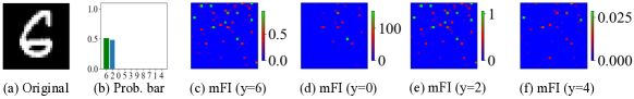
Figure 2: Pixel-level mFI maps of an MNIST image for different target classes.

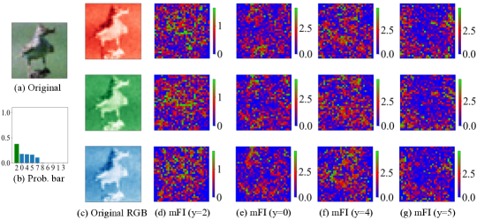
Figure 3: Pixel-level mFI maps of a CIFAR10 image’s RGB channels for different target classes. Class labels: (0, 1, 2, 3, 4, 5, 6, 7, 8, 9) = (plane, car, bird, cat, deer, dog, frog, horse, ship, truck).

III-A Illustration of the proposed mFI-PSO

We first consider two images with easy visual detection and large image-level mFI in MNIST and CIFAR10, shown in Figures 2-3 with predictive probability graphs and pixel-level mFI maps. The probability bar graphs imply candidate misclassification classes that can be used as $y_{\text{target}}$. The mFI maps indicate the vulnerability of each pixel to local perturbation and are useful to locate pixels for attack.

We evaluate the performance of Algorithm 1 (see Figure 1 (b)-(e)) in generating adversarial examples of the two images according to different requirements on $m$, $P_{\text{err}}$ and $y_{\text{target}}$. Figures 4-5 show the generated adversarial images with corresponding perturbation maps. Perturbations 1-3 consider the settings with $m=1,3,7$, respectively, and with no specifications to $P_{\text{err}}$ and $y_{\text{target}}$. For Perturbations 4-6, we only specify $P_{\text{err}}=0.5,0.75,0.99$, respectively, assign no value to $y_{\text{target}}$, and tune $m$ being the number of pixels with mFI $\geq\text{mFI}_{\text{pixel}}\in\{0.1,1\}$ and $N_{p}\in\{200,500,1000\}$ to obtain feasible solutions from PSO. Perturbations 7-9 are prespecified with $y_{\text{target}}=0,2,4$ for MNIST, and $0,4,5$ for CIFAR10, respectively, $m$ being the number of pixels with mFI $\geq 0.1$, and no value for $P_{\text{err}}$. The generated adversarial images have visually negligible differences from the originals and satisfy the prespecified requirements.

We now consider using Algorithm 2 to generate adversarial datasets. Figure 6 shows the Manhattan plots of image-level mFIs for correctly classified images. Based on the figure, for both MNIST and CIFAR10, we generate three adversarial datasets by selecting vulnerable images with image-level $\text{mFI}\geq\text{mFI}_{\text{img}}=0.2,0.1,0.01$, respectively (see Figure 1(a)). For all the sets, we set $P_{\text{target}}=0.2$ and $\text{mFI}_{\text{pixel}}=0.01$ in Algorithm 2; following [37] we set the bound of the max absolute value (i.e., the $\ell_{\infty}$ norm) of perturbations $\epsilon=0.15$ for pixel values converted onto $[0,1]$. Table II shows that the success rate of our mFI-PSO attack is enhanced as the threshold $\text{mFI}_{\text{img}}$ increases, and it is 100% when $\text{mFI}_{\text{img}}=0.2$ and is above 96.5% for MNIST and 92.5% for CIFAR10 even when $\text{mFI}_{\text{img}}$ is small as 0.01.

III-B Comparison with Related Methods

We compare the proposed mFI-PSO with five commonly-used methods, including FGSM [9], PGD [13], JSMA [15], $\ell_{\infty}$-norm CW (CW_∞) [14], and DeepFool [16]. A brief summary of the five existing methods can be found in [12]. None of the five methods can include all of the aforementioned three desirable user-customized options for crafting adversarial images. Moreover, none of them consider the perturbation intrinsically from the Riemannian manifold. In particular, similar to our pixel-level mFI map, a saliency map but based on the Jacobian matrix is utilized in the JSMA. However, as shown in [19], the mFI measure outperforms the Jacobian information in detecting vulnerable images and pixels.

We implement the five previous methods in Python using the Adversarial Robustness Toolbox (ART) from https://github.com/Trusted-AI/adversarial-robustness-toolbox. Letting pixel values transform onto $[0,1]$, following [37] we set the bound of the $\ell_{\infty}$ norm of perturbations $\epsilon=0.15$ for FGSM, PGD, CW_∞, and our mFI-PSO, but JSMA and DeepFool do not have a similar parameter to bound the magnitude of perturbations. Our mFI-PSO (Algorithm 2) is set with the same parameters as in Section III-A and the other methods are based on the default settings of the ART package. All methods are not specified with targeted classes.

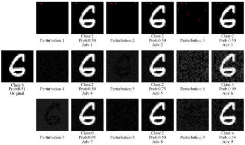
Figure 4: Adversarial examples of an MNIST image. Perturbations 1-3 are set with $m=1,3,7$, respectively; Perturbations 4-6 are with $P_{\text{err}}=0.5,0.75,0.99$, respectively; Perturbations 7-9 are with $y_{\text{target}}=0,2,4$, respectively. Perturbation maps are followed by adversarial images.

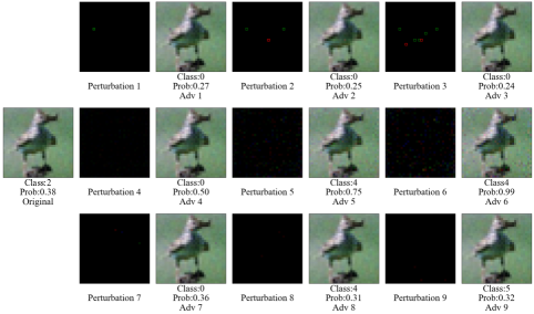
Figure 5: Adversarial examples of a CIFAR10 image. Perturbations 1-3 are set with $m{=}1,3,7$ attacked pixels (framed in the attacked channel’s color), respectively. Perturbations 4-6 are set with $P_{\text{err}}{=}0.5,0.75,0.99$, respectively. Perturbations 7-9 are set with $y_{\text{target}}{=}0,4,5$, respectively. Perturbation maps are followed by adversarial images.

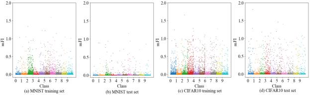
Figure 6: Manhattan plots of image-level mFIs for correctly classified images.

TABLE II: Attack success rates (in %) on correctly classified images with different image-level mFI thresholds ($\text{mFI}_{\text{img}}$)
for originally trained ResNet32.

	MNIST				CIFAR10
mFI${}_{\text{img}}$ value	0.2	0.1	0.01		0.2	0.1	0.01
CC’ed Tr./Ts.	(n=189/46)	(n=413/84)	(n=1876/325)		(n=356/229)	(n=693/385)	(n=2562/1008)
mFI-PSO	100/100	100/100	96.54/97.54		100/100	97.26/94.81	92.55/92.66
FGSM	77.78/89.13	82.08/91.67	81.82/90.46		100/100	97.40/98.96	53.16/64.19
PGD	99.47/100	99.76/100	98.61/98.38		100/100	97.98/99.74	58.70/68.35
CW∞	10.05/100	10.9/100	9.22/97.54		79.21/76.86	65.95/63.64	33.33/42.16
JSMA	0/0	0/0	0.053/1.53		63.20/60.34	65.95/57.92	57.92/64.48
	(100)/(100)	(100)/(100)	(100)/(100)		(100)/(100)	(100)/(100)	(100)/(100)
DeepFool	0.53/54.34	1.45/69.04	1.33/32.62		60.34/44.96	23.09/27.79	6.25/10.62
	(92.06)/(56.52)	(94.19)/(70.24)	(95.20)/(90.46)		(100)/(100)	(100)/(100)	(100)/(100)

• Note: The preset bound of the $\ell_{\infty}$ norm of perturbations is $\epsilon=0.15$ for pixel values converted onto $[0,1]$. JSMA and DeepFool do not have the parameter $\epsilon$, and their success rates without the $\ell_{\infty}$-norm bound are given in the parentheses. Tr. = training data, Ts. = test data, CC’ed = correctly classified.

TABLE III: Classification results of adversarially fine-tuned ResNet32.

MNIST/CIFAR10
Fine-tuned by Tr.	Accuracy in % on	Accuracy in % on	n of CC’ed Ts.
(n=60k/50k)+Adv. Tr. of	Ts. (n=10k/10k)	Adv. Ts.	with mFI$\geq$0.01
mFI-PSO (n=1811/2371)	99.78/91.63	93.06(n=317)/65.42(n=934)	132/441
FGSM (n=1535/1362)	99.65/91.77	84.69(n=294)/71.72(n=647)	169/570
PGD (n=1850/1504)	99.66/91.43	82.35(n=323)/71.55(n=689)	163/603
CW∞ (n=173/777)	99.72/91.54	93.38(n=317)/72.24(n=425)	199/615
JSMA (n=1876/2562)	99.68/91.68	91.38(n=325)/75.79(n=1008)	153/551
DeepFool (n=1786/2556)	99.60/91.77	85.03(n=294)/24.80(n=1002)	368/800

• Note: The adversarial training and test sets for each method are selected with image-level mFI $\geq 0.01$. Adv. = adversarial, Tr. = training data, Ts. = test data, CC’ed = correctly classified.

TABLE IV: Attack success rate (in %) on adversarially fine-tuned ResNet32.

MNIST/CIFAR10
	Correctly classified test images (with mFI$\geq$0.01) by the fine-tuned network of
Attacked	mFI-PSO	FGSM	PGD	CW∞	JSMA	DeepFool
by	(n=132/441)	(n=169/570)	(n=163/603)	(n=199/615)	(n=153/551)	(n=368/800)
mFI-PSO	44.06/98.87	91.72/99.47	90.80/99.50	96.48/99.19	91.50/98.37	90.52/97.75
FGSM	60.61/29.02	81.82/29.47	52.76/29.68	81.91/30.73	56.87/33.21	83.70/35.25
PGD	89.39/32.43	100/30.88	98.16/30.35	94.47/31.38	99.35/32.76	94.57/34.63
CW∞	30.30/23.13	38.46/24.91	33.74/25.21	31.66/23.58	37.91/30.13	36.96/32.50
JSMA	0/24.49	0/43.68	0/46.10	0/43.42	0/40.29	0/72.13
	(98.48/96.60)	(100/96.32)	(98.48/98.34)	(100/96.91)	(100/96.91)	(100/97.63)
DeepFool	15.91/5.90	10.06/4.91	14.11/5.80	12.27/5.04	10.45/5.63	9.51/8.13
	(87.88/88.21)	(89.35/91.40)	(89.57/89.88)	(87.94/91.54)	(91.53/88.93)	(91.30/90.13)

• Note: The preset bound of the $\ell_{\infty}$ norm of perturbations is $\epsilon=0.15$ for pixel values converted onto $[0,1]$. JSMA and DeepFool do not have parameter $\epsilon$, and their success rates without the $\ell_{\infty}$-norm bound are given in parentheses.

We first investigate the success rates of the six attack methods. We compare their attacks on the three subsets of MNIST or CIFAR10 consisting of correctly classified images with mFI $\geq\text{mFI}_{\text{img}}=0.2,0.1,0.01$, respectively. We consider these vulnerable images rather than all correctly classified images due to the slow attack speed, e.g., of JSMA. Table II reports the attack results. The mFI measure indeed benefits the success of our mFI-PSO attack. Moreover, our mFI-PSO achieves the highest attack success rate on the subsets with threshold $\text{mFI}_{\text{img}}=0.2,0.1$ for MNIST and those with $\text{mFI}_{\text{img}}=0.2,0.01$ for CIFAR10, and also has a high rate comparable to the best on the other two subsets. In particular, our mFI-PSO wins with large margins ($\geq 24\%$) on the subset of CIFAR10 with $\text{mFI}_{\text{img}}=0.01$. In contrast, CW_∞ has imbalanced performance on all the three MNIST subsets with low success rates ($\approx 10\%$) on training data but high rates ($>97.5\%$) on test data. Both JSMA and DeepFool have low success rates on these selected images if with the constraint on the magnitude of perturbations.

We then compare the six methods in adversarially fine-tuning the newtork to build more robust classifiers. For each method, the originally trained ResNet32 is additionally trained, with 30 epochs for MNIST and 80 epochs for CIFAR10, on the combined set of original training data and its adversarial dataset from the subset with $\text{mFI}\geq 0.01$. For JSMA and DeepFool, we use their adversarial datasets including the images perturbed over the 0.15 $\ell_{\infty}$-norm bound. We randomly select 1/5 of the original training data and 1/5 of the adversarial dataset as the validation set for the fine tuning. Six fine-tuned ResNet32 models are obtained for each of MNIST and CIFAR10. Table III shows the classification results of each method’s fine-tuned model on the original test data and on its own adversarial data from test images with $\text{mFI}\geq 0.01$. All fine-tuned networks perform slightly better than the originally trained network in accuracy on the original test data, and have a large improvement on corresponding adversarial datasets with accuracy over 82% for MNIST and 65% (except DeepFool with 24.8%) for CIFAR10. For more fair comparison, the table lists the sample size of vulnerable test images with $\text{mFI}\geq 0.01$ for each fine-tuned network. Our mFI-PSO dramatically reduces the sample size from 325 and 1008 to 132 and 441 for MNIST and CIFAR10, respectively, ranking the best among the six methods.

All adversarially fine-tuned networks are further attacked by all the six methods. Table IV shows the attack results for each fine-tuned network on its correctly classified test images that are vulnerable with $\text{mFI}\geq 0.01$. The network fine-tuned by our mFI-PSO generally exhibits the best defense performance over the other five networks, with most of the lowest success rates of the six attack methods and with comparable results to the best rates on its unwon items. Moreover, for the other five fine-tuned networks, our mFI-PSO attack still has high success rates over 90% on both MNIST and CIFAR10, but the other five attacks have poor success rates less than 72.2% (and below 46.2% except JSMA) on CIFAR10, and CW_∞, JSMA and DeepFool have rates below 38.5% on MNIST. For the network fine-tuned by mFI-PSO for CIFAR10, the defense against mFI-PSO is not clearly seen on its test subset of $\text{mFI}\geq 0.01$, but it is observed from the aforementioned dramatic reduced sample size (from 1008 to 441) of the vulnerable test images that have $\text{mFI}\geq 0.01$. We also use mFI-PSO to attack on the test subsets with $\text{mFI}\geq 0.01$ from the original network but correctly classified by the corresponding fine-tuned networks. Enhanced defense against mFI-PSO is observed with an attack success rate 45.51% for the mFI-PSO fine-tuned network, in contrast to the worse rates between 60.83% and 65.05% for the other five networks.

IV Conclusion

This paper introduced a novel method called mFI-PSO for adversarial image generation for DNN classifiers by accounting for the user specified number of perturbed pixels, misclassification probability, and/or targeted incorrect class. We used a mFI measure based on an “intrinsic” perturbation manifold to efficiently detect the vulnerable images and pixels to increase the attack success rate. We designed different misclassification loss functions to meet various user’s specifications and obtained the optimal perturbation by the PSO algorithm. Experiments showed good performance of our approach in generating customized adversarial samples and associated adversarial fine-tuning for DNNs and its better performance in most studied cases over some widely-used methods.

References

- [1] A. Krizhevsky, I. Sutskever, and G. E. Hinton, “Imagenet classification with deep convolutional neural networks,” in Conference on Neural Information Processing Systems, 2012, pp. 1097–1105.
- [2] K. He, X. Zhang, S. Ren, and J. Sun, “Deep residual learning for image recognition,” in CVPR, 2016, pp. 770–778.
- [3] G. Huang, Z. Liu, L. Van Der Maaten, and K. Q. Weinberger, “Densely connected convolutional networks,” in CVPR, 2017, pp. 4700–4708.
- [4] Y. Sun, D. Liang, X. Wang, and X. Tang, “Deepid3: Face recognition with very deep neural networks,” arXiv:1502.00873, 2015.
- [5] M. Bojarski, D. Del Testa, D. Dworakowski, B. Firner, B. Flepp, P. Goyal, L. D. Jackel, M. Monfort, U. Muller, J. Zhang, X. Zhang, J. Zhao, and K. Zieba, “End to end learning for self-driving cars,” arXiv:1604.07316, 2016.
- [6] C. Lyu and H. Shu, “A two-stage cascade model with variational autoencoders and attention gates for mri brain tumor segmentation,” in International MICCAI Brainlesion Workshop, 2021, pp. 435–447.
- [7] M. M. Najafabadi, F. Villanustre, T. M. Khoshgoftaar, N. Seliya, R. Wald, and E. Muharemagic, “Deep learning applications and challenges in big data analytics,” J. Big Data, vol. 2, no. 1, pp. 1–21, 2015.
- [8] C. Szegedy, W. Zaremba, I. Sutskever, J. Bruna, D. Erhan, I. Goodfellow, and R. Fergus, “Intriguing properties of neural networks,” arXiv:1312.6199, 2013.
- [9] I. J. Goodfellow, J. Shlens, and C. Szegedy, “Explaining and harnessing adversarial examples,” arXiv:1412.6572, 2014.
- [10] J. Su, D. V. Vargas, and K. Sakurai, “One pixel attack for fooling deep neural networks,” IEEE TEVC, vol. 23, no. 5, pp. 828–841, 2019.
- [11] R. R. Wiyatno, A. Xu, O. Dia, and A. de Berker, “Adversarial examples in modern machine learning: A review,” arXiv:1911.05268, 2019.
- [12] K. Ren, T. Zheng, Z. Qin, and X. Liu, “Adversarial attacks and defenses in deep learning,” Engineering, vol. 6, no. 3, pp. 346–360, 2020.
- [13] A. Madry, A. Makelov, L. Schmidt, D. Tsipras, and A. Vladu, “Towards deep learning models resistant to adversarial attacks,” arXiv:1706.06083, 2017.
- [14] N. Carlini and D. Wagner, “Towards evaluating the robustness of neural networks,” in IEEE Symp. Secur. Priv., 2017, pp. 39–57.
- [15] N. Papernot, P. McDaniel, S. Jha, M. Fredrikson, Z. B. Celik, and A. Swami, “The limitations of deep learning in adversarial settings,” in IEEE European Symposium on Security and Privacy, 2016.
- [16] S.-M. Moosavi-Dezfooli, A. Fawzi, and P. Frossard, “Deepfool: a simple and accurate method to fool deep neural networks,” in CVPR, 2016, pp. 2574–2582.
- [17] A. Kurakin, I. Goodfellow, and S. Bengio, “Adversarial examples in the physical world,” arXiv:1607.02533, 2016.
- [18] S.-M. Moosavi-Dezfooli, A. Fawzi, O. Fawzi, and P. Frossard, “Universal adversarial perturbations,” in CVPR, 2017, pp. 1765–1773.
- [19] H. Shu and H. Zhu, “Sensitivity analysis of deep neural networks,” in AAAI Conference on Artificial Intelligence, 2019, pp. 4943–4950.
- [20] R. Novak, Y. Bahri, D. A. Abolafia, J. Pennington, and J. Sohl-Dickstein, “Sensitivity and generalization in neural networks: an empirical study,” in International Conference on Learning Representations, 2018.
- [21] R. D. Cook, “Assessment of local influence,” Journal of the Royal Statistical Society Series B, vol. 48, no. 2, pp. 133–155, 1986.
- [22] H. Zhu, J. G. Ibrahim, S. Lee, and H. Zhang, “Perturbation selection and influence measures in local influence analysis,” Annals of Statistics, vol. 35, no. 6, pp. 2565–2588, 2007.
- [23] H. Zhu, J. G. Ibrahim, and N. Tang, “Bayesian influence analysis: a geometric approach,” Biometrika, vol. 98, no. 2, pp. 307–323, 2011.
- [24] A. Nazemi and P. Fieguth, “Potential adversarial samples for white-box attacks,” arXiv:1912.06409, 2019.
- [25] A. Nguyen, J. Yosinski, and J. Clune, “Deep neural networks are easily fooled: High confidence predictions for unrecognizable images,” in CVPR, 2015, pp. 427–436.
- [26] J. Kennedy and R. Eberhart, “Particle swarm optimization,” in International Conference on Neural Networks, vol. 4, 1995, pp. 1942–1948.
- [27] V. G. Gudise and G. K. Venayagamoorthy, “Comparison of particle swarm optimization and backpropagation as training algorithms for neural networks,” in IEEE Swarm Intell. Symp., 2003, pp. 110–117.
- [28] B. Warsito, H. Yasin, and A. Prahutama, “Particle swarm optimization versus gradient based methods in optimizing neural network,” Journal of Physics: Conference Series, vol. 1217, no. 1, 2019.
- [29] Q. Zhang, K. Wang, W. Zhang, and J. Hu, “Attacking black-box image classifiers with particle swarm optimization,” IEEE Access, vol. 7, pp. 158 051–158 063, 2019.
- [30] R. Mosli, M. Wright, B. Yuan, and Y. Pan, “They might not be giants: Crafting black-box adversarial examples with fewer queries using particle swarm optimization,” arXiv:1909.07490, 2019.
- [31] R. Poli, “Analysis of the publications on the applications of particle swarm optimisation,” J. Artif. Evol. Appl., vol. 2008, p. 685175, 2008.
- [32] R. Eberhart and Y. Shi, “Particle swarm optimization: developments, applications and resources,” in IEEE CEC, vol. 1, 2001, pp. 81–86.
- [33] Y. Zhang, S. Wang, and G. Ji, “A comprehensive survey on particle swarm optimization algorithm and its applications,” Mathematical Problems in Engineering, vol. 2015, p. 931256, 2015.
- [34] G. Xu, Q. Cui, X. Shi, H. Ge, Z.-H. Zhan, H. P. Lee, Y. Liang, R. Tai, and C. Wu, “Particle swarm optimization based on dimensional learning strategy,” Swarm Evol. Comput., vol. 45, pp. 33–51, 2019.
- [35] D. Meng, “Generating deep learning adversarial examples in black-box scenario,” Electronic Design Engineering, vol. 26, pp. 164–173, 2018.
- [36] D. Meng and H. Chen, “Magnet: a two-pronged defense against adversarial examples,” in ACM SIGSAC CCS, 2017, pp. 135–147.
- [37] A. Dabouei, S. Soleymani, F. Taherkhani, J. Dawson, and N. M. Nasrabadi, “Exploiting joint robustness to adversarial perturbations,” in CVPR, 2020, pp. 1122–1131.