Sorbonne Université, UMR 7589, LPTHE, F-75005, Paris, France
& CNRS, UMR 7589, LPTHE, F-75005, Paris, France

The Minor problem, namely the study of the spectrum of a principal submatrix of a Hermitian matrix taken at random on its orbit under conjugation, is revisited, with emphasis on the use of orbital integrals and on the connection with branching coefficients in the decomposition of an irreducible representation of ${\rm U}(n)$, resp. ${\rm SU}(n)$, into irreps of ${\rm U}(n-1)$, resp. ${\rm SU}(n-1)$.

1 Introduction

What we call the Minor problem deals with the following question: given an $n$-by-$n$ Hermitian matrix of given spectrum, what can be said about the eigenvalues of one of its $(n-1)\times(n-1)$ principal submatrices? This question has been thoroughly studied and answered by many authors [1, 2, 3, 4]. As several other such questions, this problem of classical linear algebra has a counterpart in the realm of representation theory [5, 6, 7], namely the determination of branching coefficients of an irreducible representation (irrep) of ${\rm U}(n)$, resp. ${\rm SU}(n)$, into irreps of ${\rm U}(n-1)$, resp. ${\rm SU}(n-1)$. The aim of this note is to review these questions and to make explicit the link, by use of orbital integrals. It is thus in the same vein as recent works on the Horn [8, 9, 10, 11, 12] or Schur-Horn [13] problems.

This paper is organized as follows. In sect. 2, I review the classical Minor problem and recall how it may be rephrased in terms of ${\rm U}(n)$ orbital integrals. This suggests a modification, that will be turn out to be natural for the case of ${\rm SU}(n)$. Sect. 3 is devoted to the issue of branching coefficients for the embeddings ${\rm U}(n-1)\subset{\rm U}(n)$ and ${\rm SU}(n-1)\subset{\rm SU}(n)$. While the former is treated by means of Gelfand–Tsetlin triangles and does not give rise to multiplicities, as well known since Weyl [14], the latter requires a new technique. This is where the modified integral introduced in sect. 2 proves useful and is shown to provide an expression of branching coefficients, see Theorem 2, which is the main result of this paper. The use of that formula as for the behaviour of branching coefficients under stretching, i.e., dilatation of the weights, is briefly discussed in the last subsection.

2 The classical problem

2.1 Notations and classical results

Let us fix notations: If $A$ is an $n\times n$ Hermitian matrix with known eigenvalues $\alpha_{1}\geq\ldots\geq\alpha_{n}$, what can be said about the eigenvalues $\beta_{1}\geq\beta_{2}\geq\ldots\geq\beta_{n-1}$ of one of its principal $(n-1)\times(n-1)$ minor submatrix (“minor” in short)?
A first trivial observation is that if we are interested in the statistics of the $\beta$’s as $A$ is taken randomly on its ${\rm U}(n)$ orbit ${\mathcal{O}}_{\alpha}$, the choice of the minor among the $n$ possible ones is immaterial, since a permutation of rows and columns of $A$ gives another matrix of the orbit.
A second, less trivial, observation is that the $\beta$’s are constrained by the celebrated Cauchy–Rayleigh interlacing Theorem:

$$\alpha_{1}\geq\beta_{1}\geq\alpha_{2}\geq\beta_{2}\geq\ldots\beta_{n-1}\geq\alpha_{n}\,.$$ (1)

For proofs, see for example [15, 4]

If $A$ is chosen at random on its orbit ${\mathcal{O}}_{\alpha}$, and uniformly in the sense of the ${\rm U}(n)$ Haar measure, what is the probability distribution (PDF) of the $\beta$’s ? This question has been answered by Baryshnikov [1], see also [3, 4]. We first observe that the problem is invariant under a global shift of all $\alpha$’s and all $\beta$’s by a same constant: indeed a translation of $A$ by $a\,\mathbb{I}_{n}$ shifts by $a$ all its eigenvalues as well as all the eigenvalues of any of its principal minors.
Let $\Delta$ denote the Vandermonde determinant: $\Delta_{n}(\alpha)=\prod_{1\leq i<j\leq n}(\alpha_{i}-\alpha_{j})$ and likewise for $\Delta_{n-1}(\beta)$.

Theorem 1 (Baryshnikov[1]).

The PDF of the $\beta$’s on its support (1) is given by

$$P(\beta\,|\,\alpha)=(n-1)!\frac{\Delta_{n-1}(\beta)}{\Delta_{n}(\alpha)}\,.$$ (2)

This result may also be recovered in terms of orbital integrals. Let

$${\mathcal{H}}^{(n)}_{\alpha}(X)=\int_{{\rm U}(n)}dUe^{{\rm tr\,}U\alpha U^{\dagger}X}$$ (3)

where $X\in H_{n}$, the space of $n\times n$ Hermitian matrices, $dU$ is the normalized Haar measure on ${\rm U}(n)$, and $\alpha$ stands here for the diagonal matrix ${\rm diag\,}(\alpha_{i})$. In terms of the eigenvalues $x_{i}$ of $X$, we write this orbital integral as ${\mathcal{H}}^{(n)}(\alpha;x)$.

The orbit ${\mathcal{O}}_{\alpha}$ carries a unique probabilistic measure, the orbital measure $\mu_{\alpha}(dA)$, $A\in{\mathcal{O}}_{\alpha}$, whose Fourier transform is ${\mathcal{H}}^{(n)}_{\alpha}(\mathrm{i\,}X)$

$$\mathbb{E}(e^{\mathrm{i\,}{\rm tr\,}AX})=\int_{{\mathcal{O}}_{\alpha}}e^{\mathrm{i\,}{\rm tr\,}AX}\mu_{\alpha}(dA)=\int_{{\rm U}(n)}dUe^{\mathrm{i\,}{\rm tr\,}U\alpha U^{\dagger}X}={\mathcal{H}}^{(n)}_{\alpha}(\mathrm{i\,}X)\,.$$

Let $\Pi$ be the projector of $H_{n}$ into $H_{n-1}$ that maps $A\in H_{n}$ onto its upper $(n-1)\times(n-1)$ minor submatrix $B$. According to the observation that the Fourier transform of the projection of the orbital measure is the restriction of the Fourier transform [4], the characteristic function of $B$ is $\phi_{B}(Y)=\phi_{A}(X_{0})$, with $X_{0}=\Pi(X)=\begin{pmatrix}Y&0\\ 0&0\end{pmatrix}\in H_{n}$, $Y\in H_{n-1}$, from which the PDF of $B$ is obtained by inverse Fourier transform

$$P(B|A)=\frac{1}{(2\pi)^{(n-1)^{2}}}\int_{H_{n-1}}dYe^{-\mathrm{i\,}{\rm tr\,}YB}\int_{{\rm U}(n)}dUe^{\mathrm{i\,}{\rm tr\,}U\alpha U^{\dagger}X_{0}}\,.$$

After reduction to eigenvalues,

$$P(\beta\,|\,\alpha)=\frac{(n-1)!}{(2\pi)^{n-1}(\prod_{1}^{n-1}p!)^{2}}\ \Delta_{n-1}^{2}(\beta)\int_{\mathbb{R}^{n-1}}dx\,\Delta_{n-1}^{2}(x){\mathcal{H}}^{(n)}(\alpha;\mathrm{i\,}(x,0)){\mathcal{H}}^{(n-1)}(\beta;\mathrm{i\,}x)^{*}\,.$$ (4)

(In physicist’s parlance, this is the overlap of the two orbital integrals.) Here and below, for $x\in\mathbb{R}^{n-1}$, $(x,0)$ denotes the corresponding vector in $\mathbb{R}^{n}$.

Making use of the explicit expressions known for ${\mathcal{H}}^{(n)}(\alpha;x)$ [16, 17], we find

$$\!\!\!\!\!\!\!\!\!P(\beta\,|\,\alpha)\!\!\! = \!\!\!C\ \Delta_{n-1}^{2}(\beta)\int_{\mathbb{R}^{n-1}}dx\Delta_{n-1}^{2}(x)\frac{\det\left(e^{\mathrm{i\,}\alpha_{i}(x,0)_{j}}\right)_{i,j=1,\cdots,n}}{\Delta_{n}(\alpha)\Delta_{n}((x,0))}\frac{\det\left(e^{-\mathrm{i\,}\beta_{i}x_{j}}\right)_{i,j=1,\cdots,n-1}}{\Delta_{n-1}(\beta)\Delta_{n-1}(x)}$$ (5)

$$= \!\!\!\frac{1}{(2\pi\mathrm{i\,})^{n-1}}\ \frac{\Delta_{n-1}(\beta)}{\Delta_{n}(\alpha)}\int_{\mathbb{R}^{n-1}}\frac{d^{n-1}x}{x_{1}x_{2}\cdots x_{n-1}}\det e^{\mathrm{i\,}\alpha_{i}(x,0)_{j}}\,\det e^{-\mathrm{i\,}\beta_{i}x_{j}}$$ (6)

since the prefactor reads

$$C=\frac{{(n-1)!}\prod_{1}^{n-1}p!\,\prod_{1}^{n-2}p!\ \mathrm{i\,}^{-n(n-1)/2+(n-1)(n-2)/2}}{(2\pi)^{n-1}(\prod_{1}^{n-1}p!)^{2}}=\frac{1}{(2\pi\mathrm{i\,})^{n-1}}$$

and since $\Delta_{n}((x,0))=(\prod_{i=1}^{n-1}x_{i})\Delta_{n-1}(x)$. Let’s write $P(\beta\,|\,\alpha)=\frac{\Delta_{n-1}(\beta)}{\Delta_{n}(\alpha)}{\mathcal{K}}(\alpha;\beta)$, hence

$${\mathcal{K}}(\alpha;\beta) = \frac{(n-1)!}{(2\pi)^{n-1}(\prod_{1}^{n-1}p!)^{2}}\ \Delta_{n}(\alpha)\Delta_{n-1}(\beta)\int_{\mathbb{R}^{n-1}}dx\Delta_{n-1}^{2}(x){\mathcal{H}}^{(n)}(\alpha;\mathrm{i\,}(x,0)){\mathcal{H}}^{(n-1)}(\beta;\mathrm{i\,}x)^{*}$$ (7)

$$= \frac{1}{(2\pi\mathrm{i\,})^{n-1}}\int_{\mathbb{R}^{n-1}}\frac{d^{n-1}x}{x_{1}x_{2}\cdots x_{n-1}}\det\big{(}e^{\mathrm{i\,}\alpha_{i}(x,0)_{j}}\big{)}_{\scriptscriptstyle 1\leq i,j\leq n}\,\det\big{(}e^{-\mathrm{i\,}\beta_{i}x_{j}}\big{)}_{\scriptscriptstyle 1\leq i,j\leq n-1}$$

in analogy with the introduction of the “volume functions” in the Horn and Schur problems [10, 11, 13]. The function ${\mathcal{K}}(\alpha;\beta)$ is then, as in these similar cases, a linear combination of products of Dirichlet integrals: $\mathrm{PP}\int\frac{e^{\mathrm{i\,}\alpha t}}{t}=\mathrm{i\,}\pi\varepsilon(\alpha)$, with $\varepsilon$ the sign function. Thus ${\mathcal{K}}(\alpha;\beta)$ must be a piecewise constant function, supported by the product of intervals given by the interlacing theorem (1).

By making use of the integral form of the Binet–Cauchy formula, (see [4]), namely

$$\int_{\mathbb{R}^{k}}\det(f_{i}(t_{j}))_{\scriptscriptstyle{1\leq i,j\leq k}}\ \det(g_{i}(t_{j}))_{\scriptscriptstyle 1\leq i,j\leq k}=k!\det\left(\int_{R}f_{i}(t)g_{j}(t)\right)_{\scriptscriptstyle 1\leq i,j\leq k}\,,$$

with here $k=n-1$, $f_{i}(t)=\frac{1}{t}(e^{\mathrm{i\,}\alpha_{i}t}-e^{\mathrm{i\,}\alpha_{n}t})$, $g_{i}(t)=e^{-\mathrm{i\,}\beta_{i}t}$, we find

$${\mathcal{K}}(\alpha;\beta) = \frac{(n-1)!}{(2\pi\mathrm{i\,})^{n-1}}\det\int_{\mathbb{R}}\frac{dt}{t}(e^{\mathrm{i\,}(\alpha_{i}-\beta_{j})t}-e^{\mathrm{i\,}(\alpha_{n}-\beta_{j})t})$$ (8)

$$= \frac{(n-1)!}{2^{n-1}}\,\det\big{(}\varepsilon(\alpha_{i}-\beta_{j})-\varepsilon(\alpha_{n}-\beta_{j})\big{)}_{1\leq i,j\leq n-1}$$ (9)

$$= \frac{(n-1)!}{2^{n-1}}\det\begin{pmatrix}\varepsilon(\alpha_{1}-\beta_{1})&\cdots&\varepsilon(\alpha_{1}-\beta_{n-1})&1\\ \varepsilon(\alpha_{2}-\beta_{1})&\cdots&\varepsilon(\alpha_{2}-\beta_{n-1})&1\\ \vdots&&&\vdots\\ \varepsilon(\alpha_{n}-\beta_{1})&\cdots&\varepsilon(\alpha_{n}-\beta_{n-1})&1\end{pmatrix}\,.$$ (10)

Equ. (9) just reproduces a result by Olshanksi [3], since the difference $\big{(}\varepsilon(\alpha_{i}-\beta_{j})-\varepsilon(\alpha_{n}-\beta_{j})\big{)}$ appearing there is nothing else than twice the characteristic function of the interval $[\alpha_{n},\alpha_{i}]$, denoted $M_{2}(\beta_{j};\alpha_{n},\alpha_{i})$ in [4]. Finally, it may be shown that the determinant in (10) equals $2^{n-1}$ times the characteristic function of (1), so that the piecewise constant function ${\mathcal{K}}$ is just $(n-1)!$ on its support, in agreement with (2), see [3, 4].

Remark. The previous considerations extend to projections of matrix $A$ onto a smaller minor $k\times k$ submatrix, see [2, 3, 4].

2.2 A modified integral

In this section, we introduce a modification of the integral (7) that will be suited in our later study of ${\rm SU}(n)$ branching rules. We first change variables in ${\mathcal{K}}$, introducing the spacings $\gamma_{i}=\beta_{i}-\beta_{n-1}$, $i=1,\cdots,n-2$ and rewrite (7) as

$${\mathcal{K}}(\alpha;\beta)=\frac{1}{(2\pi\mathrm{i\,})^{n-1}}\int_{\mathbb{R}^{n-1}}\frac{d^{n-1}x}{x_{1}x_{2}\cdots x_{n-1}}e^{-\mathrm{i\,}\beta_{n-1}\sum_{j=1}^{n-1}x_{j}}\,\det\big{(}e^{\mathrm{i\,}\alpha_{i}(x,0)_{j}}\big{)}_{\scriptscriptstyle 1\leq i,j\leq n}\,\det\big{(}e^{-\mathrm{i\,}\gamma_{i}x_{j}}\big{)}_{\scriptscriptstyle 1\leq i,j\leq n-1}\,,$$

where by convention $\gamma_{n-1}=0$. We then integrate over $\beta_{n-1}$ (while introducing a $1/(n-1)!$ prefactor for later convenience), and define

$$\!\!\!\!\!\widebar{\mathcal{K}}(\alpha;\gamma)\!\!\! := \!\!\!\frac{1}{(n-1)!}\int d\beta_{n-1}{\mathcal{K}}(\alpha;\gamma+\beta_{n-1})$$

$$= \!\!\!\frac{(2\pi)}{(n-1)!(2\pi\mathrm{i\,})^{n-1}}\int_{\mathbb{R}^{n-1}}\frac{d^{n-1}x}{x_{1}x_{2}\cdots x_{n-1}}\ \delta\Big{(}\sum_{1}^{n-1}x_{j}\Big{)}\det\big{(}e^{\mathrm{i\,}\alpha_{i}(x,0)_{j}}\big{)}_{\scriptscriptstyle 1\leq i,j\leq n}\,\det\big{(}e^{-\mathrm{i\,}\gamma_{i}x_{j}}\big{)}_{\scriptscriptstyle 1\leq i,j\leq n-1}\,.$$

Remark. Although it depends only on the spacings $\gamma$, the function $\widebar{\mathcal{K}}$ is not directly related to the PDF of the spacings in the original Minor problem. Its introduction is rather motivated by its connection with the $\mathfrak{su}(n)$ Lie algebra, see below sect. 3.2.

Thus integrating ${\mathcal{K}}$ over $\beta_{n-1}$ amounts to considering a modified integral, where in (7) we integrate on the $(n-2)$-dimensional hyperplane $\sum_{i=1}^{n-1}x_{i}=0$. Hence an alternative definition of $\widebar{\mathcal{K}}$ is

$$\widebar{\mathcal{K}}(\alpha;\gamma)=\frac{\Delta_{n}(\alpha)\Delta_{n-1}(\gamma)}{(2\pi)^{n-2}(\prod_{1}^{n-1}p!)^{2}}\int_{\mathbb{R}^{n-1}}dx\,\delta\Big{(}\sum_{1}^{n-1}x_{j}\Big{)}\,\Delta_{n-1}^{2}(x){\mathcal{H}}^{(n)}(\alpha;\mathrm{i\,}(x,0)){\mathcal{H}}^{(n-1)}(\gamma;\mathrm{i\,}x)^{*}\,,$$ (12)

an expression that we use later in sect. 3.2. A more explicit expression is

$$\!\!\!\!\!\widebar{\mathcal{K}}(\alpha;\gamma)={\textstyle\frac{2\pi}{(2\pi\mathrm{i\,})^{n-1}(n-1)!}}\ \int_{\sum_{1}^{n-1}\!\!x_{i}=0}\ \,\frac{dx}{x_{1}x_{2}\cdots x_{n-1}}\det\left({\scriptstyle e^{\mathrm{i\,}\alpha_{i}x_{1}},e^{\mathrm{i\,}\alpha_{i}x_{2}},\cdots,e^{\mathrm{i\,}\alpha_{i}x_{n-1}},1}\right)_{\scriptscriptstyle 1\leq i\leq n-1}\,\det\big{(}e^{-\mathrm{i\,}\gamma_{i}x_{j}}\big{)}_{\scriptscriptstyle 1\leq i,j\leq n-1}$$ (13)

and we note that, because of the constraint $\sum_{i=1}^{n-1}x_{i}=0$, this expression is invariant by a global shift of all $\alpha_{i}$. We may use that invariance to choose $\alpha_{n}=0$, a choice that will be natural in the application to ${\rm SU}(n)$ representations. We conclude that $\widebar{\mathcal{K}}(\alpha,{\gamma})$ is a function of two sets of variables, a $n$-plet $\alpha$ with $\alpha_{n}=0$, and a $(n-1)$-plet ${\gamma}$ with ${\gamma}_{n-1}=0$. As is clear from (2.2), $\widebar{\mathcal{K}}$ may be extended to a function of the unordered $\alpha$’s and ${\gamma}$’s, odd under the action of the symmetric group ${\mathcal{S}}_{n}$, i.e., the ${\rm SU}(n)$ Weyl group, acting on $\alpha$ by $w(\alpha)_{i}=\alpha_{w(i)}-\alpha_{w(n)}$, $i=1,\cdots,n$, $w\in{\mathcal{S}}_{n}$, and likewise odd under the action of ${\mathcal{S}}_{n-1}$ on ${\gamma}_{i}$, $i=1,\cdots,n-1$.

Expanding the two determinants and using once again the Dirichlet integrals $\mathrm{PP}\int\frac{e^{\mathrm{i\,}at}}{t^{r}}=\mathrm{i\,}\pi\frac{(\mathrm{i\,}a)^{r-1}}{(r-1)!}\varepsilon(a)$, one finds that $\widebar{\mathcal{K}}(\alpha;{\gamma})$, a combination of convoluted box splines, is a piece-wise linear function of differentiability class $C^{0}$. Its support is the polytope defined by the inequalities (recall that by convention $\alpha_{n}=0$)

$$\max_{1\leq i\leq n-1}(\alpha_{i+1}-{\gamma}_{i})\leq\min_{1\leq i\leq n-1}(\alpha_{i}-{\gamma}_{i})$$ (14)

that guarantee that there exist $\beta_{n-1}$ satisfying the simultaneous inequalities (1), i.e.,

$$\alpha_{i+1}\leq\beta_{i}={\gamma}_{i}+\beta_{n-1}\leq\alpha_{i}\,,\ \mathrm{for\ all}\ i=1,\cdots,n-1\,.$$ (15)

The maximal value (in the dominant sector) of $\widebar{\mathcal{K}}$, for fixed $\alpha$, is readily derived from (2.2), where we are integrating the function ${\mathcal{K}}/(n-1)!$ equal to 1 on its support, over $\beta_{n-1}$, subject to the $n-1$ conditions (15), hence

$$\max_{{\gamma}}\widebar{\mathcal{K}}(\alpha;{\gamma})=\min_{1\leq i\leq n-1}(\alpha_{i}-\alpha_{i+1})\,.$$ (16)

Let $\epsilon_{w}$ denote the signature of permutation $w\in{\mathcal{S}}_{n}$. For $n=3$ the function $\widebar{\mathcal{K}}$ reads

$$\widebar{\mathcal{K}}(\alpha;{\gamma}) = \frac{1}{2}\Big{(}\left|\alpha_{1}-{\gamma}_{1}\right|-\left|\alpha_{1}-\alpha_{2}-{\gamma}_{1}\right|-\left|\alpha_{2}-{\gamma}_{1}\right|\Big{)}-({\gamma}_{1}\mapsto-{\gamma}_{1})$$

$$= \frac{1}{2}\sum_{w\in{\mathcal{S}}_{3}}\epsilon_{w}|w(\alpha)_{1}-{\gamma}_{1}|$$

which is an odd continuous function of ${\gamma}_{1}$, vanishing for ${\gamma}_{1}\notin(-\alpha_{1},\alpha_{1})$, constant and equal to its extremum value $\pm\min(\alpha_{1}-\alpha_{2},\alpha_{2})$ for $|{\gamma}_{1}|\in[\min(\alpha_{1}-\alpha_{2},\alpha_{2}),\max(\alpha_{1}-\alpha_{2},\alpha_{2}))$, and linear in between, see Fig. 1.
For $n=4$, let $w(\bar{\alpha})_{i}=\alpha_{w(i)}-\alpha_{w(n)}$,

$$\psi(\alpha;{\gamma}):=\varepsilon(\alpha_{1}-{\gamma}_{1})\Big{(}|\alpha_{2}-{\gamma}_{2}|-|\alpha_{3}-{\gamma}_{2}|-|\alpha_{1}-\alpha_{2}-{\gamma}_{1}+{\gamma}_{2}|+|\alpha_{1}-\alpha_{3}-{\gamma}_{1}+{\gamma}_{2}|\Big{)}$$ (18)

then

$$\widebar{\mathcal{K}}(\alpha;{\gamma})=\frac{1}{8}\sum_{w\in{\mathcal{S}}_{4}}\epsilon_{w}\psi(w(\alpha);{\gamma})$$ (19)

$\widebar{\mathcal{K}}(\alpha;{\gamma})$ has a support in the dominant sector defined by the inequalities

$$(\alpha_{2}-\alpha_{3})\leq{\gamma}_{1}\leq\alpha_{1}\,,\qquad 0\leq{\gamma}_{2}\leq\alpha_{2}\,,\qquad 0\leq{\gamma}_{1}-{\gamma}_{2}\leq\alpha_{1}-\alpha_{3}\,,$$ (20)

and a maximal value equal to $\min(\alpha_{1}-\alpha_{2},\alpha_{2}-\alpha_{3},\alpha_{3})$. Its graph has an Aztec pyramid shape, see Fig. 2.

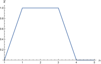
Figure 1: The $\widebar{\mathcal{K}}$ function for $n=3$, $\alpha=\{4,1,0\}$ and ${\gamma}_{1}\geq{\gamma}_{2}=0$.

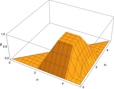
Figure 2: The $\widebar{\mathcal{K}}$ function for $n=4$ and $\alpha=\{5,3,1,0\}$, in the ${\gamma}_{1}\geq{\gamma}_{2}\geq{\gamma}_{3}=0$ sector.

3 The “quantum” problem

In this section, we consider the restriction of the group ${\rm U}(n)$, resp. ${\rm SU}(n)$, to its subgroup ${\rm U}(n-1)$, resp. ${\rm SU}(n-1)$, and the ensuing decomposition of their representations. For definiteness, the restriction of ${\rm SU}(n)$ to ${\rm SU}(n-1)$ we have in mind results from projecting out the simple root $\boldsymbol{\alpha}_{n-1}$ in the dual of the Lie algebra $\mathfrak{su}(n)$, and likewise for ${\rm U}(n)$.

3.1 Gelfand–Tsetlin patterns

Just like in the cases of the Horn or of the Schur problem, the Minor problem is the classical counterpart of a “quantum” problem in representation theory. Given a highest weight (h.w.) irreducible representation (irrep) $V^{(n)}_{\alpha}$ of ${\rm U}(n)$, which irreps $V^{(n-1)}_{\beta}$ of ${\rm U}(n-1)$ occur and with which multiplicities, in the restriction of ${\rm U}(n)$ to ${\rm U}(n-1)$? That problem too is well known, is important in physical applications (see for example [18, 19]), and may be solved by a variety of methods. Here we first recall how to make use of Gelfand–Tsetlin triangles, i.e., triangular patterns

$$\begin{array}[]{rlcrlcrlcrlcrl}x_{1}^{(n)}=\alpha_{1}&\cdots&&\cdots&&\cdots&x_{n}^{(n)}=\alpha_{n}\\ &x_{1}^{(n-1)}&\cdots&&\cdots&x_{n-1}^{(n-1)}&\\ &&\ddots&&\mathinner{\mkern 2.0mu\raise 1.0pt\hbox{.}\mkern 3.0mu\raise 4.0pt\hbox{.}\mkern 1.0mu\raise 7.0pt\hbox{.}}&&&\\ &&&x_{1}^{(1)}&&&\end{array}$$

subject to the inequalities

$$x_{i}^{(j+1)}\geq x_{i}^{(j)}\geq x_{i+1}^{(j+1)}\ ,\qquad{1\leq i,j\leq n-1}\,.$$ (21)

In the present context, the $\alpha$’s denote the lengths of the rows of the Young diagram associated with the irrep $V^{(n)}_{\alpha}$. The number of solutions of the inequalities (21) gives the dimension of the irrep

$$\dim(V^{(n)}_{\alpha})=\#\{x_{i}^{(j)}|\mathrm{solutions\ of\ }(\ref{GTineq})\}\,.$$

The values $\beta_{i}=x_{i}^{(n-1)}$, $1\leq i\leq n-1$, appearing in the second row of the triangle give the lengths of rows of the Young diagrams of the possible representations $V^{(n-1)}_{\beta}$ of ${\rm U}(n-1)$. Given those numbers, the number of solutions $x_{i}^{(j)}$, $1\leq i,j\leq n-2$ satisfying (21) is the dimension of the representation of ${\rm U}(n-1)$. Thus we have the sum-rule

$$\dim(V^{(n)}_{\alpha}) = \#\{x_{i}^{(j)}|\mathrm{solutions\ of\ }(\ref{GTineq}),\ x^{(n)}=\alpha\}\$$

$$= \sum_{\beta}\#\{x_{i}^{(j)}|\mathrm{solutions\ of\ }(\ref{GTineq}),\,\ x^{(n)}=\alpha,\,\ x^{(n-1)}=\beta\}\ =\sum_{\beta}\dim(V^{(n-1)}_{\beta})\,,$$

which is consistent with the multiplicity 1 of each $V^{(n-1)}_{\beta}$ appearing in the decomposition, a classical result in representation theory [14, 20, 21], see also chapter 8 in [22]. Thus one sees that the $\beta$’s satisfy the inequalities (1) and one may say that the branching coefficient, equal to 0 or 1, is given

$$\mathrm{br}_{\alpha}(\beta)=K(\alpha;\beta)$$ (23)

with the convention that the discontinuous function ${\mathcal{K}}$ is assigned the value $1$ throughout its support, including its boundaries.

Going from ${\rm U}(n)$ to ${\rm SU}(n)$, we have to restrict to Young diagrams with less than $n$ rows, or equivalently, to reduce Young diagrams with $n$ rows by deleting all columns of height $n$. Starting from an irrep of ${\rm SU}(n)$, we apply to it the procedure above, and then remove the columns of height $n-1$.

Example in ${\rm SU}(3)$. Take for $\alpha$ the adjoint representation, i.e., $\alpha=\{2,1,0\}$. The possible $\beta$ satisfying (1) are written in red in what follows

$$2\geq{\color[rgb]{1,0,0}2}\geq 1\geq{\color[rgb]{1,0,0}1}\geq 0 \quad{\rm i.e.,\/}\ \beta=\{2,1\}\equiv\{1,0\}$$ (24)

$$2\geq{\color[rgb]{1,0,0}1}\geq 1\geq{\color[rgb]{1,0,0}1}\geq 0 \quad{\rm i.e.,\/}\ \beta=\{1,1\}\equiv\{0,0\}$$ (25)

$$2\geq{\color[rgb]{1,0,0}2}\geq 1\geq{\color[rgb]{1,0,0}0}\geq 0 \quad{\rm i.e.,\/}\ \beta=\{2,0\}$$ (26)

$$2\geq{\color[rgb]{1,0,0}1}\geq 1\geq{\color[rgb]{1,0,0}0}\geq 0 \quad{\rm i.e.,\/}\ \beta=\{1,0\}$$ (27)

where two $\beta$ are regarded as equivalent if their Young diagrams differ by a number of columns of height $n-1=2$. Hence in ${\rm SU}(2)\subset{\rm SU}(3)$, we write

$$\mathrm{br}_{\alpha}(\beta)=1,2,1\quad\mathrm{for}\ \beta=\{0,0\},\ \{1,0\},\ \{2,0\}$$ (28)

and we check the sum-rule on dimensions: $8=1+2\times 2+3$. Note that removing columns of height $n-1$ in the Young diagram associated with $\beta$ amounts to focusing on spacings between the $\beta$’s, which points to the relevance of our function $\widebar{\mathcal{K}}$.

To summarize, in the “quantum”, ${\rm U}(n)$-representation theoretic, problem, the $\beta$’s are the integer points interlacing the $\alpha$’s and come with multiplicity 1, while in the ${\rm SU}(n)$ case, non trivial multiplicities may occur and the interlacing property no longer applies. In the next subsection, we show that the latter multiplicities are given by the function $\widebar{\mathcal{K}}$ of sect. 2.2.

3.2 A $\widebar{\mathcal{K}}-\mathrm{br}$ relation

The multiplicities occurring in the ${\rm SU}(n-1)\subset{\rm SU}(n)$ problem may be expressed in terms of characters by the integral

$$\mathrm{br}_{\alpha}({\gamma})=\int Dt\,\chi^{(n)}_{\alpha}(e^{\mathrm{i\,}(t,0)})\big{(}\chi^{(n-1)}_{\gamma}(e^{\mathrm{i\,}t})\big{)}^{*}$$ (29)

which computes the projection of the ${\rm SU}(n)$ character $\chi^{(n)}_{\alpha}$ restricted to the Cartan torus of ${\rm SU}(n-1)$ onto the ${\rm SU}(n-1)$ character $\chi^{(n-1)}_{\gamma}$. There, $Dt$ stands for the Haar measure on the Cartan torus $\mathbb{T}_{n-1}$ of ${\rm SU}(n-1)$

$$Dt=\frac{|\widehat{\Delta}_{n-1}(e^{\mathrm{i\,}t})|^{2}}{(2\pi)^{n-2}(n-1)!}dt$$

where we use the notations

$$\widehat{\Delta}_{n-1}(e^{\mathrm{i\,}t}):=\prod_{\boldsymbol{\alpha}>0}\big{(}e^{\mathrm{i\,}\langle\boldsymbol{\alpha},t\rangle/2}-e^{-\mathrm{i\,}\langle\boldsymbol{\alpha},t\rangle/2}\big{)}\,,\qquad\mathrm{and}\qquad\Delta_{n-1}(t):=\prod_{\boldsymbol{\alpha}>0}\langle\boldsymbol{\alpha},t\rangle\,,$$

$\boldsymbol{\alpha}$ the positive roots of $\mathfrak{su}(n-1)$, and $dt$ is the Lebesgue measure on $\mathbb{T}_{n-1}$.

Theorem 2.

The branching coefficient, that gives the multiplicity of the irrep of ${\rm SU}(n-1)$ of h.w. ${\gamma}$ in the decomposition of the irrep of ${\rm SU}(n)$ of h.w. $\alpha$, is

$$\mathrm{br}_{\alpha}({\gamma})=\widebar{\mathcal{K}}(\alpha+\rho_{n};{\gamma}+\rho_{n-1})$$ (30)

with $\rho_{n}$ the Weyl vector of the algebra $\mathfrak{su}(n)$, and $\rho_{n-1}$ that of $\mathfrak{su}(n-1)$.

Proof. We recall Kirillov’s relation between a ${\rm SU}(n)$ character and the orbital integral:

$$\chi^{(n)}_{\alpha}(e^{\mathrm{i\,}t})=\dim V_{\alpha}\frac{\Delta_{n}(\mathrm{i\,}t)}{\widehat{\Delta}_{n}(e^{\mathrm{i\,}t})}{\mathcal{H}}^{(n)}({\alpha+\rho_{n}}\,;\mathrm{i\,}t)$$ (31)

with $\dim V_{\alpha}=\frac{\Delta_{n}(\alpha+\rho_{n})}{\Delta_{n}(\rho)}$. Plugging in (12) the expression (31) and the analogous one for $\mathfrak{su}(n-1)$ leads to

$$\!\!\!\!\!\widebar{\mathcal{K}}(\alpha+\rho_{n};{\gamma}+\rho_{n-1})\!\!\! = \!\!\!\frac{\Delta_{n}(\alpha+\rho_{n})\Delta_{n-1}({\gamma}+\rho_{n-1})}{(2\pi)^{n-2}(\prod_{1}^{n-1}p!)^{2}}\int_{\mathbb{R}^{n-2}}\!\!\!\!\!\!dt\,\Delta_{n-1}^{2}(t){\mathcal{H}}^{(n)}({\alpha+\rho_{n}};\mathrm{i\,}(t,0)){\mathcal{H}}^{(n-1)}({{\gamma}+\rho_{n-1}};\mathrm{i\,}t)^{*}$$

$$= \frac{\prod_{p=1}^{n-1}p!\prod_{p=1}^{n-2}p!}{(2\pi)^{n-2}(\prod_{1}^{n-1}p!)^{2}}\int_{\mathbb{R}^{n-2}}\!\!\!dt\,\Delta_{n-1}^{2}(t)\frac{\widehat{\Delta}_{n}(e^{\mathrm{i\,}(t,0)})\widehat{\Delta}_{n-1}(e^{\mathrm{i\,}t})^{*}}{\Delta_{n}(\mathrm{i\,}(t,0))\Delta_{n-1}(\mathrm{i\,}t)^{*}}\chi^{(n)}_{\alpha}(e^{\mathrm{i\,}(t,0)})\chi^{(n-1)}_{\gamma}(e^{\mathrm{i\,}t})^{*}$$

$$= \frac{\mathrm{i\,}^{-(n-1)}}{(2\pi)^{n-2}(n-1)!}\int_{\mathbb{R}^{n-2}}\!\!\!dt\,|\widehat{\Delta}_{n-1}(e^{\mathrm{i\,}t})|^{2}\chi^{(n)}_{\alpha}(e^{\mathrm{i\,}(t,0)})\chi^{(n-1)}_{\gamma}(e^{\mathrm{i\,}t})^{*}\frac{\Delta_{n-1}(t)}{\Delta_{n}((t,0))}\frac{\widehat{\Delta}_{n}(e^{\mathrm{i\,}(t,0)})}{\widehat{\Delta}_{n-1}(e^{\mathrm{i\,}t})}$$

$$= \mathrm{i\,}^{-(n-1)}\,\int_{\mathbb{T}_{n-1}}\!\!\!Dt\,\sum_{\delta\in 2\pi Q^{\vee}}\chi^{(n)}_{\alpha}(e^{\mathrm{i\,}(t+\delta,0)})\chi^{(n-1)}_{\gamma}(e^{\mathrm{i\,}(t+\delta)})^{*}\frac{\Delta_{n-1}(t+\delta)}{\Delta_{n}((t+\delta,0))}\frac{\widehat{\Delta}_{n}(e^{\mathrm{i\,}(t+\delta,0)})}{\widehat{\Delta}_{n-1}(e^{\mathrm{i\,}(t+\delta)})}$$

where the integration is now carried out on the Cartan torus of ${\rm SU}(n-1)$, $\mathbb{T}_{n-1}=\mathbb{R}^{n-2}/(2\pi Q^{\vee})$, $Q^{\vee}$ the $(n-2)$-dimensional coroot lattice of ${\rm SU}(n-1)$, which is, in the present simply laced case, isomorphic to the root lattice. Only the ratio $\frac{\Delta_{n-1}(t+\delta)}{\Delta_{n}((t+\delta,0))}$ depends on $\delta$ and the summation can be carried out with the result that

$$\mathrm{i\,}^{-(n-1)}\frac{\widehat{\Delta}_{n}(e^{\mathrm{i\,}(t,0)})}{\widehat{\Delta}_{n-1}(e^{\mathrm{i\,}t})}\sum_{\delta\in 2\pi Q^{\vee}}\frac{\Delta_{n-1}(t+\delta)}{\Delta_{n}((t+\delta,0))}=1\,.$$ (32)

Indeed, if we write $(t,0)$ in the $\mathfrak{su}(n)$ root basis: $(t,0)=\sum_{j=1}^{n-2}a_{j}\boldsymbol{\alpha}_{j}$ (with no component on $\boldsymbol{\alpha}_{n-1})$,

$$\frac{\widehat{\Delta}_{n}(e^{\mathrm{i\,}(t,0)})}{\widehat{\Delta}_{n-1}(e^{\mathrm{i\,}t})}=-(2\mathrm{i\,})^{n-1}\sin\frac{a_{1}}{2}\left(\prod_{i=1}^{n-3}\sin\frac{a_{i+1}-a_{i}}{2}\right)\,\sin\frac{a_{n-2}}{2}\,,$$ (33)

(on which it is clear that it is invariant under $a_{i}\mapsto a_{i}+p_{i}(2\pi)$, $p_{i}\in\mathbb{Z}$), while

$$\frac{\Delta_{n}((t,0))}{\Delta_{n-1}(t)}=-{a_{1}}\left(\prod_{i=1}^{n-3}(a_{i+1}-a_{i})\right)\,{a_{n-2}}$$ (34)

and the identity (32) follows from a repeated use of

$$\sum_{p=-\infty}^{\infty}\frac{1}{(a+2\pi p)(b-a-2\pi p)}=\frac{1}{2b}\,\frac{\sin\frac{b}{2}}{\sin\frac{a}{2}\sin\frac{b-a}{2}}\,$$

in the telescopic product (34). $\Box$

Remark. The proof above follows closely similar proofs in [10, 13] that relate the classical Horn or Horn–Schur problems to the computation of Littlewood–Richardson or Kostka coefficients. However, in contrast with those cases, here the r.h.s is a single term, rather than a linear combination involving a convolution.

Together with the results of the end of sect. 2.2, Theorem 2 has immediate consequences:

Corollary 1.

The number of irreps of ${\rm SU}(n-1)$ appearing in the decomposition of the irrep of ${\rm SU}(n)$ of h.w. $\alpha$ (with $\alpha_{n}=0$) is equal to the number of integer points in the polytope defined by the inequalities (14), where $\alpha$ is changed into $\alpha+\rho_{n}$, namely

$$\#\{{\gamma}\in\mathbb{Z}_{+}^{n-1}\ |\ {\gamma}_{1}\geq\cdots\geq{\gamma}_{n-1}\geq 0\ ,\quad\max_{1\leq i\leq n-1}(\alpha_{i+1}+n-i-1-{\gamma}_{i})\leq\min_{1\leq i\leq n-1}(\alpha_{i}+n-i-{\gamma}_{i})\}\,.$$

Here as before, the $\alpha_{i}$ are the Young coordinates of the h.w. $\alpha$, i.e., , the lengths of the rows of its Young diagram.

On the other hand, eq. (30) together with (16) gives the maximal value of a branching coefficient of a given $\alpha$

$$\max_{{\gamma}}\mathrm{br}_{\alpha}({\gamma})=\min_{i}((\alpha+\rho_{n})_{i}-(\alpha+\rho_{n})_{i+1})=\min_{i}(\alpha_{i}-\alpha_{i+1})+1$$ (35)

and note that $\alpha_{i}-\alpha_{i+1}$ is just the $i$-th Dynkin component of the weight $\alpha$.

Corollary 2.

The largest multiplicity (branching coefficient) that occurs in the branching of an irrep of ${\rm SU}(n)$ of h.w. $\alpha$ into irreps of ${\rm SU}(n-1)$ is 1 plus the smallest Dynkin component of $\alpha$.

Examples. Take $n=3$ and the example considered in sect. 3.1. $\alpha=\{2,1,0\}$, i.e., $(1,1)$ in Dynkin components, $\alpha+\rho_{3}=\{4,2,0\}$, ${\gamma}\in\{\{0,0\},\,\{1,0\},\,\{2,0\}\},\ {\gamma}+\rho_{2}\in\{\{1,0\},\,\{2,0\},\,\{3,0\}\}$, one finds with the formula (2.2): $\widebar{\mathcal{K}}(\alpha+\rho_{3};{\gamma}+\rho_{2})=1,2,1$ in agreement with (28).
For $n=4$, take $\alpha=\{6,4,3,0\}$, i.e., $(2,1,3)$ in Dynkin components, one finds the following decomposition into 18 ${\rm SU}(3)$ weights

$$\{6,4,3,0\}\!\!\!\!\! = \!\!\!\!\!(1,3)_{2}\oplus(1,2)_{2}\oplus(1,1)_{2}\oplus(1,0)_{1}\oplus(0,4)_{1}\oplus(0,3)_{1}\oplus(0,2)_{1}\oplus(0,1)_{1}\oplus(2,3)_{2}\qquad$$

$$\!\!\!\!\!\oplus(2,2)_{2}\oplus(2,1)_{2}\oplus(2,0)_{1}\oplus(1,4)_{1}\oplus(3,3)_{1}\oplus(3,2)_{1}\oplus(3,1)_{1}\oplus(3,0)_{1}\oplus(2,4)_{1}$$

in terms of Dynkin components, and with the multiplicity appended as a subscript.

3.3 Stretching

The relation (30) is also well suited for the study of the behaviour of branching coefficients under “stretching”. From (35) we learn that the growth is at most linear

$$\mathrm{br}_{s\alpha}(s{\gamma})\leq s\min(\alpha_{i}-\alpha_{i+1})+1\,.$$

For example, for $n=3$, with Dynkin components, $\mathrm{br}_{(s,s)}(s)=s+1$ since

$$\mathrm{br}_{(s,s)}(s)=\widebar{\mathcal{K}}(\{2s+2,s+1,0\};\{s+1,0\})=(s+1)\widebar{\mathcal{K}}(\{2,1,0\};\{1,0\})=s+1$$

while for $\mathrm{br}_{(s,s)}(s-1)$ or $\mathrm{br}_{(s,s)}(2s)$, we are not probing the function on its plateau and its behaviour is not always linear in $s$:

$$\widebar{\mathcal{K}}(\{2s+2,s+1,0\};\{{\gamma}_{1},0\})=\begin{cases}{\gamma}_{1}&\mathrm{if}\quad 0\leq{\gamma}_{1}\leq s+1\\ 2(s+1)-{\gamma}_{1}&\mathrm{if}\quad s+1\leq{\gamma}_{1}\leq 2(s+1)\end{cases}$$

whence $\mathrm{br}_{(s,s)}(s-1)=\widebar{\mathcal{K}}(\{2s+2,s+1,0\};\{s,0\})=s$ and $\mathrm{br}_{(s,s)}(2s)=\widebar{\mathcal{K}}(\{2s+2,s+1,0\};\{2s+1,0\})=1$.

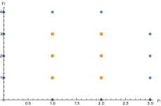
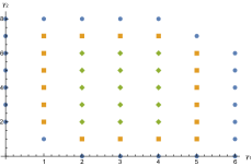
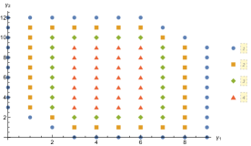
Figure 3: Weights in the ${\gamma}$-plane (in Dynkin components) appearing in the decomposition of the weight $\alpha=s\{6,4,3,0\}\equiv s(2,1,3)$ of ${\rm SU}(4)$, for $s=1,2,3$. Markers of different colours code for multiplicities from 1 to 4.

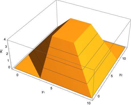
Figure 4: The $\widebar{\mathcal{K}}$ function for $n=4$, $\alpha+\rho_{4}=\{21,14,10,0\}=3\{6,4,3,0\}+\{3,2,1,0\}$ and ${\gamma}_{1},{\gamma}_{2}$ are Dynkin components. The cross-sections at altitude $1,2,3,4$ match the successive layers of multiplicities in Fig. 3, right.

Similar behaviours occur for branching coefficients in higher rank cases, due to the linear growth of the maximal value (16). For ${\rm SU}(3)\subset{\rm SU}(4)$, the points of increasing multiplicity form a matriochka pattern, see Fig. 3, in a way already encountered in the Littlewood–Richardson coefficients of ${\rm SU}(3)$, [23]. This pattern just reproduces the cross-sections of increasing altitude of the Aztec pyramid of Fig. 4.

References

- [1] Yu. Baryshnikov, GUEs and queues, Probab. Theory Relat. Fields 119 (2001) 256–274
- [2] Yu.A. Neretin, Rayleigh triangles and non-matrix interpolation of matrix beta-integrals, Sbornik, Mathematics 194 (2003) 515–540
- [3] G. Olshanski, Projection of orbital measures, Gelfand–Tsetlin polytopes, and splines, Journal of Lie Theory 23 (2013) 1011–1022
- [4] J. Faraut, Rayleigh theorem, projection of orbital measures, and spline functions, Adv. Pure Appl. Math. 6 (2015) 261–283
- [5] G.J. Heckman, Projections of Orbits and Asymptotic Behavior of Multiplicities for Compact Connected Lie Groups, Invent. Math. 67 (1982), 333–356
- [6] V. Guillemin, E. Lerman and S. Sternberg, Symplectic Fibrations and Multiplicity Diagrams, Cambridge Univ. P. 1996
- [7] M. Duflo and M. Vergne, Kirillov’s formula and Guillemin–Sternberg conjecture, Comptes-rendus Académie des Sciences 349 (2011) 1213-1217, http://arxiv.org/abs/1110.0987
- [8] J.-B. Zuber, Horn’s problem and Harish-Chandra’s integrals. Probability distribution functions, Ann. Inst. Henri Poincaré Comb. Phys. Interact., 5 (2018), 309-338, http://arxiv.org/abs/1705.01186
- [9] R. Coquereaux and J.-B. Zuber, Ann. Inst. Henri Poincaré Comb. Phys. Interact. 5 (2018) 339-386, http://arxiv.org/abs/1706.02793
- [10] R. Coquereaux, C. McSwiggen and J.-B. Zuber, On Horn’s Problem and its Volume Function, Commun. Math. Phys. 376 (2020) 2409–2439, https://doi.org/10.1007/s00220-019-03646-7, http://arxiv.org/abs/1904.00752
- [11] R. Coquereaux, C. McSwiggen and J.-B. Zuber, Revisiting Horn’s Problem, Dedicated to the memory of Vladimir Rittenberg, J. Stat. Mech. (2019) 094018 , https://doi.org/10.1088/1742-5468/ab3bc2, http://arxiv.org/abs/1905.09662
- [12] C. McSwiggen, Box splines, tensor product multiplicities and the volume function, http://arxiv.org/abs/1909.12278
- [13] R. Coquereaux and J.-B. Zuber, On Schur problem and Kostka numbers, to appear in B. Dubrovin’s memorial volume, Proceedings of Symposia in Pure Mathematics (PSPUM), AMS, http://arxiv.org/abs/2001.08046
- [14] H. Weyl, The Theory of Groups and Quantum Mechanics, Methuen and Co., Ltd., London, 1931, reprinted Dover Publications, Inc., New York, 1950.
-
[15]
https://fr.wikipedia.org/wiki/Th%C3%A9or%C3%A8me_min-max_de_Courant-Fischer
Steve Fisk, A very short proof of Cauchy’s interlace theorem for eigenvalues of Hermitian matrices, Amer. Math. Monthly, 112 (2005) 118, http://arxiv.org/abs/math/0502408 - [16] Harish-Chandra, Differential Operators on a Semisimple Algebra, Amer. J. Math. 79 (1957), 87–120
- [17] C. Itzykson and J.-B. Zuber, The planar approximation II, J. Math. Phys. 21 (1980), 411–421
- [18] H. Georgi, Lie algebras in particle physics, Benjamin 1982
- [19] P. Di Francesco, P. Mathieu and D. Sénéchal, Conformal Field Theory, Springer 1996
- [20] F. D. Murnaghan, The Theory of Group Representations, Johns Hopkins Press, Baltimore 1938
- [21] D.P. Zhelobenko, The classical groups. Spectral analysis of their finite-dimensional representations, Russian Math. Surveys 17 (1962), 1 9
- [22] R. Goodman and N.R. Wallach, Symmetries, Representations and Invariants, Graduate Texts in Mathematics, Springer 2009
- [23] R. Coquereaux and J.-B. Zuber, Conjugation properties of tensor product multiplicities, J. Phys. A: Math. Theor. 47 (2014) 455202, http://arxiv.org/abs/1405.4887