Learning DAGs without imposing acyclicity

Abstract

We explore if it is possible to learn a directed acyclic graph (DAG) from data without imposing explicitly the acyclicity constraint. In particular, for Gaussian distributions, we frame structural learning as a sparse matrix factorization problem and we empirically show that solving an $\ell_{1}$-penalized optimization yields to good recovery of the true graph and, in general, to almost-DAG graphs. Moreover, this approach is computationally efficient and is not affected by the explosion of combinatorial complexity as in classical structural learning algorithms.

1 Introduction

A vast literature exists on learning DAGs from data. Usually algorithms are classified as constrained based or score based (Scutari et al., 2019). Score-based methods optimize some score function over the space of DAGs, usually employing some heuristic such as greedy search. Constraint-based methods, such as the PC algorithm (Spirtes et al., 1993; Colombo and Maathuis, 2014), use instead conditional independence testing to prune edges from the graph and apply sets of rules to direct some of the remaining edges and find an estimate of the Markov equivalence class (Chickering, 1995). Recently, Zheng et al. (2018, 2020) proposed the use of optimization techniques to estimate DAG structures by writing the acyclicity condition of a directed graph as a smooth constraints for the weighted adjacency matrix. All the methods available in the literature for structure recovery of DAGs impose somehow the acyclicity condition. We propose instead to consider the estimation of DAGs as a general sparse matrix-factorization problem for the inverse covariance matrix arising from linear structural equation models (Drton, 2018; Spirtes, 1995; Richardson, 1997). We estimate such sparse matrix-factorization solving an $\ell_{1}$-penalized minus log-likelihood minimization using a straightforward proximal gradient method. The proposed method takes inspiration from optimization-based algorithms for structure recovery such as the graphical lasso (Friedman et al., 2007) and especially the method proposed in Varando and Hansen (2020) where covariance matrices are parametrized as solutions of, eventually sparse, Lyapunov equations. In Section 4 we perform a simulation study and observe that the proposed method is competitive with classical approaches from the literature on the recovery of the true graph, while being generally faster.

A fortran implementation of the method, together with examples of its usage within R and python, is available at github.com/gherardovarando/nodag.

2 Linear structural equation models

A linear structural equation model (SEM) with independent Gaussian noise is a statistical model for a $p$-dimensional random vector $X$ defined as the solution of

$$X=\Lambda^{t}X+\epsilon,$$ (1)

where we assume that $\epsilon$ is a $p$-dimensional zero-mean independent Gaussian noise and $\Lambda\in\mathbb{R}^{p\times p}$. If $I-\Lambda$ is invertible, equation (1) implies the covariance parametrization (Drton, 2018)

$$\operatorname{Var}(X)=(I-\Lambda)^{-t}\Omega(I-\Lambda)^{-1}$$ (2)

where $\Omega=\operatorname{Var}(\epsilon)$ is a diagonal positive definite matrix. The connection between Gaussian Bayesian networks and the system of equations (1) is immediate if we assume that the matrix $\Lambda$ has a sparsity structure compatible with a given directed acyclic graph ${G}$.

Inverting equation 2 we obtain the factorization of the inverse covariance matrix as

$$\operatorname{Var}(X)^{-1}=(I-\Lambda)\Omega^{-1}(I-\Lambda)^{t}=AA^{t},$$ (3)

with $A=(I-\Lambda){\Omega}^{-{1}/{2}}$ having the same off-diagonal sparsity pattern as $\Lambda$.

Parametrizing the multivariate Gaussian distribution with the inverse covariance matrix, we can define the linear structural equation model with independent Gaussian noise, and associate graph ${G}$, as the family of normal distributions $\mathcal{N}(\mu,\Sigma)$ with $\Sigma^{-1}$ in

$$\mathcal{M}_{{G}}=\left\{AA^{t}\text{ s.t. }A\in\mathbb{R}^{p\times p}\text{ invertible and }A_{ij}=0\text{ if }i\not\rightarrow j\text{ in }{G}\right\}$$

In particular when the graph ${G}$ is acyclic the set of inverse covariance matrices $\mathcal{M}_{G}$ corresponds to Gaussian Bayesian network models.

2.1 Markov equivalence classes

It is known that in general is not possible to recover completely the graph $G$ from observational data, since different graphs give rise to the same statistical model, in which case we say that the two graphs are equivalent (Heckerman et al., 1994). The equivalence classes obtained considering the quotient of the space of directed graphs with respect to the above equivalence are called Markov equivalence classes. In particular, if the graph $G$ is a DAG its Markov equivalence class consists of all DAGs having the same skeleton and exactly the same v-structures (Andersson et al., 1997; Heckerman et al., 1994). A completely partially directed acyclic graph (CPDAG) can be used to represent the Markov equivalence class for DAGs (Andersson et al., 1997). A CPDAG is a partially directed graph where directed edges represent edges that have the same directions in all DAGs belonging to the Markov class, while undirected edges are drawn where there exists DAGs in the Markov equivalence class with different directions for a given edge.

3 Structure recovery

Considering the factorization of the precision matrix (3) it is immediate to consider the following minimization problem for the $\ell_{1}$-penalized minus log-likelihood

$$\begin{array}[]{ll}\text{minimize }&-2\log\det(A)+\operatorname{trace}(A^{t}\hat{R}A)+\lambda||A||_{1}\\ \text{subject to }&A\in\mathbb{R}^{p\times p}\text{ invertible}\end{array},$$ (4)

where $\hat{R}$ is the empirical correlation matrix estimated from the data.

Solving the above problem, we estimate a sparse factorization of the inverse covariance matrix and the estimated graph can be read directly from the non-zero entries of the minimizer.

Remark 1

The proposed structural estimation is a general estimation for linear SEM, including models with cycles. We focus on the recovery of DAGs mainly because the literature on learning acyclic graphs is more extense and more methods are available.

3.1 Solving the optimization

Various methods can be used to solve problem (4), we present here a very simple approach using a proximal gradient method (Bach et al., 2012; Parikh and Boyd, 2014) similar to the algorithm proposed in Varando and Hansen (2020).

The proximal gradient is a method applicable to minimization problems where the objective function has a decomposition into a sum of two functions of which one is differentiable. In particular, the objective function of problem (4) can be written as $f(A)+g(A)$ where $f(A)=-2\log\det(A)+\operatorname{trace}(A^{t}\hat{R}A)$ and $g(A)=||A||_{1}$, with $f$ differentiable.

The proximal gradient algorithm consists of iterations of the form

$$A^{(k)}=\mathcal{S}_{s\lambda}\left(A^{(k)}-s\nabla f\right)$$

where the soft-thresholding $\mathcal{S}_{t}(A)_{ij}=\operatorname{sign}(A_{ij})\left(|A_{ij}|-t\right)_{+}$ is the proximal operator for the $\ell_{1}$-penalization and $\nabla f(A)=2\hat{R}A-2A^{-1}$. At each iteration the step size $s$ is selected using the line search proposed in Beck and Tabulle (2010).

A complete description of the algorithm and its implementation is given in the Appendix A.

Example 1

We simulate $1000$ synthetic observations from a Gaussian Bayesian network with associated DAG given in Figure 1 (a). The graph estimated solving the optimization problem (4) is shown in Figure 1 (b). We can observe that all the v-structures in the true DAG are correctly recovered. Nevertheless, the estimated graph is not a valid DAG since it contains the directed cycle $7\leftrightarrow 8$.

Figure 1: True DAG (a) and estimated graph with $\lambda=0.2$ (b).

4 Simulations

We perform a simulation study to explore how the proposed method behaves with respect to the recovery of the true graph. Data is generated from Gaussian Bayesian networks with known structure similarly to Colombo and Maathuis (2014), in particular random DAGs with $p\in\{5,10,20,50,100\}$ nodes are generated with independent probability of edges $\frac{k}{p}$, $k=1,2,3,4$. Coefficients for the linear regression of each variable on its parents are independent realizations of a uniform distribution between $0.1$ and $1$, and the noise distribution is either standard Gaussian or exponential with rate parameter equal to $1$. For each combination of $p$, $k$ and noise distribution we generate $20$ DAGs and subsequently sample $n=100,1000,10000$ observations from the induced structural equation models.

We apply our proposed method (nodag) by solving the optimization problem (4) with $\lambda=0.1,0.2,0.3$. For comparison, we consider three classical structural-recovery algorithms: the order independent PC (Colombo and Maathuis, 2014), the greedy equivalent search (Chickering, 2003), and an hill-climbing search. The PC algorithm (pc) and the greedy equivalent search (ges) are implemented in the pcalg R package (Kalisch et al., 2012), while the hill-climbing search with tabu (tabu) is available in the bnlearn R package (Scutari, 2010). For the pc method we use the Gaussian conditional independence test via Fisher’s Z and various significance levels ($0.01$, $0.005$ and $0.001$). Both ges and tabu methods optimize the Bayesian information criterion, as default in their implementations. For the tabu we also fix the maximum cardinality of the parent set to $10$ to limit the computational complexity.

The pc algorithm and the greedy equivalent search estimate a representation of the Markov equivalence class while the hill-climbing search and the proposed nodag method estimate a directed graph.

4.1 Results

Similarly to Colombo and Maathuis (2014) we evaluate the estimated graphs using the F1 score (f1), false positive rate (fpr) and true positive rate (tpr) with respect to the true skeleton recovery. Figure 2 shows the average metrics for the skeleton recovery for the different algorithms. We observe that the nodag method obtains, in general, comparable results to the literature algorithms, while performing clearly better in the small sample size with respect to skeleton recovery and slightly worse in the large sample size and small graphs.

Evaluating edge directions is more tricky, since different DAGs with the same skeleton can be Markov equivalent (see Section 2.1), and moreover algorithms can output estimated directed or partially directed graphs. We chose to report structural Hamming distance to both the true DAG (shd-graph) and the true CPDAG (shd-cpdag) in Figure 3. We can see that the proposed method is on average superior to other algorithms with respect to the recovery of the true DAG. As for the skeleton recovery, nodag performs worst in the large sample and small system dimensions. As we showed in Example 1 the graphs estimated by nodag have,sometimes, a double edge $i\leftrightarrow j$, and we have observed that this happens especially when the true CPDAG have the corresponding undirected edge $i-j$.

In general the value of the penalization coefficient $\lambda$ obtaining the optimal results is, as expected, dependent on the sample size, but on average it does not seem to be too much sensitive.

In Figure 4 we report the average execution time for the different methods. The nodag method is shown to outperform all the other methods from a computational speed prospective, especially for large sample and system sizes.

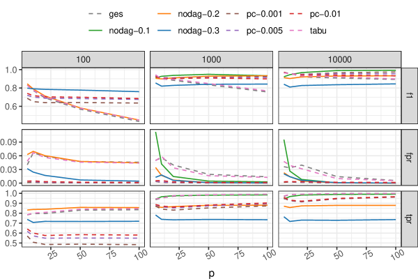
Figure 2: Average F1 score, true positive rate and false positive rate for the recovery of the skeleton. Different algorithms in different colours, the proposed nodag method with solid lines and algorithms from the literature dashed. Results for nodag-0.1 are not shown for $n=100$ to improve readability.

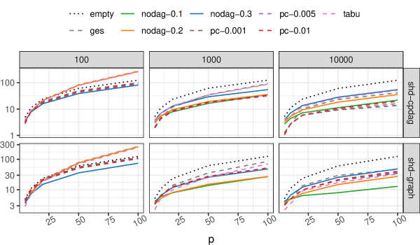
Figure 3: Average structural hamming distances with respect to the true CPDAG (shd-cpdag) and to the true DAG (shd-graph). Different algorithms in different colours, the proposed nodag method with solid lines and algorithms from the literature dashed. The distance with respect to the empty graph is shown with black dotted lines. Results for nodag-0.1 are not shown for $n=100$ to improve readability.

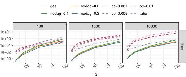
Figure 4: Average execution time for different algorithms (colours), the proposed nodag method with solid lines and algorithms from the literature dashed.

5 Protein signaling network

As an example of real-data application we consider the dataset from Sachs et al. (2005) largely used (Friedman et al., 2007; Meinshausen et al., 2016; Zheng et al., 2018; Varando and Hansen, 2020) in the graphical models and causal discovery literature.

Data consist of observations of phosphorylated proteins and phospholipids ($p=11$) from cells under different conditions ($n=7466$).

We estimate the graph representing the protein-signaling network with our nodag method with $\lambda=0.2$ (Figure 5). The nodag method estimates a graph without cycles and with $12$ edges of which $4$ are also present in the consensus network (Sachs et al., 2005). Tow estimated edges, jnk $\rightarrow$ pkc and mek $\rightarrow$ raf, appear with reversed direction in the consensus network while others (jnk $\rightarrow$ p38, akt $\rightarrow$ erk, akt $\rightarrow$ mek) appear in the graph estimated from other methods in the literature (Meinshausen et al., 2016; Varando and Hansen, 2020).

Figure 5: Graph estimated as the support of $A^{*}$ from solving the optimization problem (4) with $\lambda=0.2$. In blue edges that are present in the conventionally accepted network (Sachs et al., 2005).

6 Discussion

We have framed the problem of learning DAGs in the larger class of linear structural equation models and we have shown that a simple approach based on optimization techniques and without any acyclicity constraints is able to obtain similar recovery performances than state-of-the-art algorithms, see Figures 2 and 3.

The proposed nodag is also considerably faster than classical constraint-based and score-based methods (Figure 4). By avoiding the acyclicity constraint we are able to use a standard proximal gradient algorithm over a matrix $A\in\mathbb{R}^{p\times p}$ and thus the computational cost of the method depends only on the size of the system ($p$) and not on the sparsity level or the sample size.

Moreover, the output of the nodag method parametrizes the inverse covariance matrix and thus provides an estimation of the parameters of the model, contrary to constraint-based algorithms. In particular, from the estimation of the $A$ matrix is possible to recover an estimate of the coefficient matrix $\Lambda$ in equation (3).

6.1 Feature directions

The nodag method estimates linear SEM without acyclicity constraints and thus it would be interesting to empirically test its performance in the recovery of SEM with cycles.

As for lasso (Friedman et al., 2010), graphical lasso (Friedman et al., 2007) and other $\ell_{1}$-penalized methods (Varando and Hansen, 2020) it is straightforward to extend the method to estimate the regularization path for a sequence of decreasing $\lambda$ values and thus being able to perform data-driven selection for the regularization coefficient. The good computational complexity make it feasible to combine the proposed algorithm with stability selection methods Meinshausen and Bühlmann (2010) and, by not imposing acyclicity, it allows to simply average matrices estimated from bootstrapped or sub-sampled data.

Finally, from a strictly computational point of view, it would be interesting to explore ways to speed up both the computations and the convergence of Algorithm 1. The sparsity of matrix $A$ in Algorithm 1 could probably be used to speed up or avoid the computation of its LU decomposition, this would in turn decrease the cost-per-iteration. Accelerated gradient-like methods could be applied to improve the speed of convergence (Beck and Teboulle, 2009), thus reducing the number of iterations needed to converge.

6.2 Reproducibility

The code and instructions to reproduce the examples, the simulation study and the real-world application are available at https://github.com/gherardovarando/nodag_experiments.

Acknowledgments

This work was supported by VILLUM FONDEN (grant 13358).

Appendix A Algorithm implementation

Algorithm 1 details the pseudocode of the proposed proximal method to solve problem 4. Each iteration of the algorithm consists basically in the gradient computation and the line search loop where the gradient descent and the proximal operator are applied for decreasingly small step sizes until the descent and the Beck and Tabulle (2010) conditions are met. The algorithm terminates when the difference of the objective function computed in the last two iterations is less than a specified tolerance ($\varepsilon$) or when the maximum number of iterations ($M$) has been reached. The LU factorization of $A$, used to compute both the log-determinant and the inverse, is performed with the LAPACK implementation Anderson et al. (1999) using partial pivoting.

The fortran code implementing algorithm 1 is available at github.com/gherardovarando/nodag.

Algorithm 1 Proximal gradient algorithm for minimization of $\ell_{1}$-penalized minus log-likelihood

0:  $\hat{R}$ the empirical correlation matrix,     $M\in\mathbb{N}$, $\varepsilon>0,\lambda>0,\alpha\in(0,1)$

1:  initialize $k=0$, $A=L=U=I$

2:  $f=\sum_{i=1}^{p}\hat{R}_{ii}$

3:  $g=0$

4:  repeat

5:     increase iteration counter $k=k+1$

6:     compute $A^{-1}$ using the LU decomposition

7:     obtain the gradient ${D}=2\hat{R}A-2A^{-1}$

8:     copy $A$ into $A^{\prime}$

9:     $f^{\prime}=f$, $g^{\prime}=g$

10:     $s=1$

11:     loop

12:        ${A}={A^{\prime}}-sD$

13:        soft thresholding $A$ at level $s\lambda$

14:        $L,U=$ LU decomposition of $A$

15:        compute $\hat{R}A$

16:        $f=-2\sum_{i=1}^{p}\log(U_{ii})+\sum_{i,j=1}^{p}A_{ij}\left(\hat{R}A\right)_{ij}$

17:        $g=\lambda||A||_{1}$

18:        $\nu=\sum_{i,j}^{p}\frac{1}{2s}(A_{ij}-A^{\prime}_{ij})^{2}+(A_{ij}-A_{ij}^{\prime})D_{ij}$

19:        if $f\leq f^{\prime}+\nu$ and $f+g\leq f^{\prime}+g^{\prime}$ then

20:           break

21:        else

22:           $s=\alpha s$

23:        end if

24:     end loop

25:     $\delta=(f^{\prime}+g^{\prime}-f-g)$

26:  until $k>M$ or $\delta<\varepsilon$

26:  $A$, $f$, $\delta$, $k$

References

- Anderson et al. [1999] E. Anderson, Z. Bai, C. Bischof, S. Blackford, J. Demmel, J. Dongarra, J. Du Croz, A. Greenbaum, S. Hammarling, A. McKenney, and D. Sorensen. LAPACK Users’ Guide. Society for Industrial and Applied Mathematics, Philadelphia, PA, third edition, 1999.
- Andersson et al. [1997] Steen A. Andersson, David Madigan, and Michael D. Perlman. A characterization of Markov equivalence classes for acyclic digraphs. Ann. Statist., 25(2):505–541, 04 1997.
- Bach et al. [2012] Francis Bach, Rodolphe Jenatton, Julien Mairal, and Guillaume Obozinski. Optimization with sparsity-inducing penalties. Found. Trends Mach. Learn., 4(1):1–106, 2012. ISSN 1935-8237.
- Beck and Tabulle [2010] A. Beck and M. Tabulle. Gradient-based algorithms with applications to signal recovery problems. In D. Palomar and Y. Eldar, editors, Convex Optimization in Signal Processing and Communications, pages 42–88. Cambridge University Press, 2010.
- Beck and Teboulle [2009] Amir Beck and Marc Teboulle. A fast iterative shrinkage-thresholding algorithm for linear inverse problems. SIAM Journal on Imaging Sciences, 2(1):183–202, 2009.
- Chickering [1995] David Maxwell Chickering. A transformational characterization of equivalent Bayesian network structures. In Proceedings of the Eleventh Conference on Uncertainty in Artificial Intelligence, UAI’95, page 87–98, San Francisco, CA, USA, 1995. Morgan Kaufmann Publishers Inc.
- Chickering [2003] David Maxwell Chickering. Optimal structure identification with greedy search. Journal of Machine Learning Research, 3:507–554, 2003.
- Colombo and Maathuis [2014] Diego Colombo and Marloes H. Maathuis. Order-independent constraint-based causal structure learning. Journal of Machine Learning Research, 15(116):3921–3962, 2014.
- Drton [2018] Mathias Drton. Algebraic problems in structural equation modeling. In The 50th Anniversary of Gröbner Bases, pages 35–86, Tokyo, Japan, 2018. Mathematical Society of Japan.
- Friedman et al. [2007] J. Friedman, T. Hastie, and R. Tibshirani. Sparse inverse covariance estimation with the graphical lasso. Biostatistics, 9(3):432–441, 12 2007.
- Friedman et al. [2010] J. Friedman, T. Hastie, and R. Tibshirani. Regularization paths for generalized linear models via coordinate descent. Journal of Statistical Software, 33(1):1–22, 2010.
- Heckerman et al. [1994] David Heckerman, Dan Geiger, and David M. Chickering. Learning Bayesian networks: The combination of knowledge and statistical data. In Ramon Lopez [de Mantaras] and David Poole, editors, Uncertainty Proceedings 1994, pages 293 – 301. Morgan Kaufmann, San Francisco (CA), 1994.
- Kalisch et al. [2012] Markus Kalisch, Martin Mächler, Diego Colombo, Marloes H. Maathuis, and Peter Bühlmann. Causal inference using graphical models with the R package pcalg. Journal of Statistical Software, 47(11):1–26, 2012.
- Meinshausen and Bühlmann [2010] N. Meinshausen and P. Bühlmann. Stability selection. Journal of the Royal Statistical Society: Series B (Statistical Methodology), 72(4):417–473, 2010.
- Meinshausen et al. [2016] N. Meinshausen, A. Hauser, J. M. Mooij, J. Peters, P. Versteeg, and P. Bühlmann. Methods for causal inference from gene perturbation experiments and validation. Proceedings of the National Academy of Sciences, 113(27):7361–7368, 2016.
- Parikh and Boyd [2014] N. Parikh and S. Boyd. Proximal algorithms. Found. Trends Optim., 1(3):127–239, 2014.
- Richardson [1997] Thomas Richardson. A characterization of markov equivalence for directed cyclic graphs. International Journal of Approximate Reasoning, 17(2):107 – 162, 1997. Uncertainty in AI (UAI’96) Conference.
- Sachs et al. [2005] K. Sachs, O. Perez, D. Pe’er, D. A. Lauffenburger, and G. P. Nolan. Causal protein-signaling networks derived from multiparameter single-cell data. Science, 308(5721):523–529, 2005.
- Scutari [2010] Marco Scutari. Learning bayesian networks with the bnlearn R package. Journal of Statistical Software, 35(3):1–22, 2010. doi: 10.18637/jss.v035.i03.
- Scutari et al. [2019] Marco Scutari, Catharina Elisabeth Graafland, and José Manuel Gutiérrez. Who learns better Bayesian network structures: Accuracy and speed of structure learning algorithms. International Journal of Approximate Reasoning, 115:235 – 253, 2019.
- Spirtes [1995] Peter Spirtes. Directed cyclic graphical representations of feedback models. In Proceedings of the Eleventh Conference on Uncertainty in Artificial Intelligence, 02 1995.
- Spirtes et al. [1993] Peter Spirtes, Clark Glymour, and Richard Scheines. Causation, Prediction, and Search, volume 81. 01 1993.
- Varando and Hansen [2020] Gherardo Varando and Niels Ricchard Hansen. Graphical continuous Lyapunov models. Submitted, 2020.
- Zheng et al. [2018] Xun Zheng, Bryon Aragam, Pradeep Ravikumar, and Eric P. Xing. DAGs with NO TEARS: Continuous Optimization for Structure Learning. In Advances in Neural Information Processing Systems, 2018.
- Zheng et al. [2020] Xun Zheng, Chen Dan, Bryon Aragam, Pradeep Ravikumar, and Eric P. Xing. Learning sparse nonparametric DAGs. In International Conference on Artificial Intelligence and Statistics, 2020.