Bayesian optimization for modular black-box systems with switching costs
Abstract
Most existing black-box optimization methods assume that all variables in the system being optimized have equal cost and can change freely at each iteration. However, in many real-world systems, inputs are passed through a sequence of different operations or modules, making variables in earlier stages of processing more costly to update. Such structure induces a dynamic cost from switching variables in the early parts of a data processing pipeline. In this work, we propose a new algorithm for switch-cost-aware optimization called Lazy Modular Bayesian Optimization (LaMBO). This method efficiently identifies the global optimum while minimizing cost through a passive change of variables in early modules. The method is theoretically grounded which achieves a vanishing regret regularized with switching cost. We apply LaMBO to multiple synthetic functions and a three-stage image segmentation pipeline used in a neuroimaging task, where we obtain promising improvements over existing cost-aware Bayesian optimization algorithms. Our results demonstrate that LaMBO is an effective strategy for black-box optimization capable of minimizing switching costs.
1 Introduction
Bayesian optimization (BO) [Snoek et al., 2012, Srinivas et al., 2010, Mockus et al., 1978] is a popular technique that is used to optimize unknown black-box systems. Such systems arise in a wide range of applications ranging from robotics [Berkenkamp et al., 2016] and sensor networks [Garnett et al., 2010], to hyperparameter tuning in machine learning [Bergstra et al., 2011, Frazier, 2018]. In the black-box setting, the underlying function that maps variables to a reward (loss) is unknown and is instead queried. BO methods find ways to tackle this challenging setting by approximating the unknown function with a Gaussian process (GP) [Rasmussen, 2003] and updating this belief on the fly to decide which sample to generate next.
Unfortunately, when trying to optimize a complex black-box system, the cost of generating a sample can often be prohibitive. Here, costs could represent the amount of time, energy, or resources required to generate a black-box sample (i.e., test a new hyperparameter parameter configuration of interest). To account for costs to update different variables, or overall cost constraints, a wide range of different cost-aware and multi-resolution sampling strategies ranging from batch optimization [González et al., 2016, Kathuria et al., 2016], multi-fidelity model [Kandasamy et al., 2016, 2017], multi-objective optimization [Abdolshah et al., 2019], to dynamic programming [Lam and Willcox, 2017, Lam et al., 2016] have been developed over the past decade.
While the underlying black-box function that we want to optimize may be unknown, many real-world systems have costs with specific structure that are known ahead of time. An important yet simple abstraction of many systems encountered in practice is that they process their inputs through a sequence of modules, where the outputs from one module to the next are chained together. For instance, in many scientific applications like genomics [Davis-Turak et al., 2017] and neuroimaging [Abraham et al., 2014, Johnson et al., 2019], generating an output (sample) often involves running high-dimensional inputs through multiple stages (modules) of processing, and each module has unique hyperparameters that must be optimized. When making updates in these types of sequential systems, it becomes much more costly to update a variable at an earlier stage of processing because we must take into account the fact that all operations in subsequent stages must be rerun. Not only does this sequential structure affect the cost, but it also gives rise to switching costs, where the cost depends on which variables are modified between consecutive iterations. However, most of these methods are agnostic to additional information about the structure of the underlying costs in the system, and thus are too aggressive in changing variables across modules.
In light of these motivations, we introduce a new algorithm for black-box optimization called Lazy Modular Bayesian Optimization (LaMBO). This method leverages modular and sequential structure in a system to reduce overall cumulative costs during optimization. To quantify the cost of switching in these cases, we model the cost of each query as the aggregation of cost needed to rerun modules from the first step where a variable must be updated. By encouraging the optimization method to be lazy, analytically we show that LaMBO achieves a sublinear rate in a notion of switching-cost regularized regret. We also empirically evaluate the performance of the proposed method by applying LaMBO to a number of synthetic datasets and neuroimaging problem where the aim is to tune a modular pipeline for 3D reconstruction of neuroanatomical structures from slices of 2D images [Lee et al., 2019, Johnson et al., 2019]. Our empirical results show that hyperparameters in this three-stage system can be optimized to optimality jointly over multiple modules within 1.4 hours compared with 5.6 hours obtained from the best of the alternatives. These results point to the fact that leveraging system structure, and dynamic switching costs, can be advantageous for optimizing multi-stage black-box systems.
Summary of Contributions.
The contributions of this work are as follows: (i) In Section 3, we formulate a novel Bayesian optimization problem with switching-cost constraints, and propose the algorithm LaMBO to solve the problem in systems with modular structure. To the best of our knowledge, this is the first attempt to leverage modular system structure in the design of a cost-efficient algorithm for black-box optimization. (ii) In Section 4, we establish theoretical guarantees of LaMBO by proving a regularized regret bound taking switching-cost consumption into consideration using techniques from both the multi-armed bandit and Bayesian optimization literature. (iii) In Section 5, we apply our method to synthetic functions and to a 3D brain-image-segmentation task. We empirically demonstrate that the method can efficiently solve switch-cost-aware optimization across modular compositions of functions.
2 Background and Related Work
2.1 Bayesian Optimization
Black-box optimization methods aim to find the global minimum of an unknown function with only a few queries. Let and be the optimal function value and optimizer, respectively. Standard algorithms seek to produce a sequence of inputs that result in (potentially) noisy observations such that will approach the optimal value quickly. A common choice to measure performance of a candidate algorithm is the cumulative regret:
| (1) |
Among the many different approaches for black-box optimization, BO is a celebrated probabilistic method whose statistical inferences are tractable and theoretically grounded. It uses a Gaussian process (GP) prior on the distribution of the unknown function , which is characterized by a mean function and a kernel function . Let , , and represent the noise variance. In this case, we can update the posterior with simple closed-form formulas:
| (2) |
Common classes of selection algorithms that use a BO framework include the: Upper Confidence Bound (UCB) [Srinivas et al., 2010], Expected-Improvement (EI) [Mockus, 1982], and entropy search [Wang and Jegelka, 2017] algorithms. At the heart of all of these methods is the design of an acquisition function that is used to select the next evaluation point, i.e., . The acquisition function allows flexibility in trading-off between exploration and exploitation and are constructed using the posterior statistics. In this paper, we will adopt the UCB acquisition function due to its simplicity and success in both theory and practice. The GP-UCB acquisition function is given by
| (3) |
where is a design parameter that controls the amount of exploration in the algorithm.
2.2 Slowly Moving Bandit Algorithm
To incorporate switching costs into a BO sampling strategy, we adopt [Koren et al., 2017b] on solving a multi-armed bandit problem with switching costs. In this setting, optimization is formulated into a arm-selection problem where optimal variables (arms) are selected from a set to minimize an unknown loss function . At each iteration , we can query an oracle to measure the loss (inverse reward) by pulling arm . In the switch-cost-aware case, there is a cost metric which incurs cost when switching between arms from to . The objective is to minimize a linear combination of the loss and switching cost. In [Koren et al., 2017b], the authors propose the slowly moving bandit algorithm (SMB) to tackle the problem with a general cost metric. Here, we extend the idea to the setting of black-box optimization.
SMB is based on a multiplicative update strategy [Auer et al., 2002] that encodes the cost of switching between arms in a tree; each arm is a leaf and the cost to switch from one arm to another is encoded in the distance from their corresponding leafs in the tree. At each iteration , SMB chooses an arm according to a probability distribution conditioned on the level of the tree (the root is level ) selected at the last iteration. We will make the sampling distribution precise momentarily. The distribution is then updated with a standard multiplicative update rule , where is the learning rate and is the estimated loss. Compared with basic bandit algorithms, there are two key modifications in SMB. First, it uses conditional sampling to encourage slow switching. This constrains the arm selection to be the close to the previous choice, where distance is embedded in the tree’s structure. Formally, an arm is drawn according to the following conditional distribution , where is a random level chosen at previous iteration, and denotes the leaves (arms) that belong to the subtree rooted at level which has as one of its leaves. This ensures that remains in some small subtree as in the previous iteration. Second, to utilize the classic multiplicative method, SMB makes sure that in average the conditional sampling is equivalent to direct sampling by modifying the loss estimators as,
| (4) | ||||
| (5) |
where is an unmodified loss estimator for algorithms without switching cost, and are i.i.d. uniform random variables in . For the purpose of self-contained, we include the pseudo-code of SMB in Supp. D.
2.3 Related work
The closest framework to ours in Bayesian optimization is the cost-aware Bayesian optimization, where instead of trying to minimize a function using the fewest samples, the methods strive to find the optimizer with least cumulative cost. The most standard method [Snoek et al., 2012, Lee et al., 2020] measures the acquisition function in the unit of the cost , where denotes the cost function and is some trade-off parameter. Another approach is to impose explicit cumulative budget constraints [Lam et al., 2016, Lam and Willcox, 2017], where the authors have used dynamic programming-based approaches. While many of these algorithms have proposed cost-efficient optimization strategies under static costs, the scenario with the switching cost where deviating from a previous action induces larger costs, has not been well-understood in the literature.
Multi-fidelity strategies [Kandasamy et al., 2017, Poloczek et al., 2017, Wu et al., 2020, McLeod et al., 2017] are also popular choices in which the decision maker is allowed to choose an additional fidelity parameter that controls the accuracy and the cost for function evaluations. In the sense that across subsequent resolutions there are correlations or structure in the costs of different parameters. On the surface, it seems our problem can be easily cast under the framework. However, as the dependencies on the accuracy of function approximation to variables in different modules are non-separable, one can not map a module to a fidelity. Another cost efficient BO approach similar to our work is process constrained BO [Vellanki et al., 2017], where some variables are not allowed to change due to constraints from physical system. CA-MOBO [Abdolshah et al., 2019] is also a cost-aware strategy which uses the framework of multi-objective optimization. It generalizes the UCB method to multi-dimensional outputs seeking a sweet spot in the trade-off between cost consumption and optimization accuracy. Our work differs from theirs as we are allowed to probe variables anytime but may incur different cost when changing sets of variables in different modules, and we consider costs arising from switching variables.
The switching cost optimization has been studied in multi-armed bandit literature [Kalai and Vempala, 2005, Koren et al., 2017a, b, Dekel et al., 2014, Feldman et al., 2016]. However, the arms are assumed to be uncorrelated, while in our work we assume strong dependency and leverage it by using Gaussian surrogate to explore multi-arms simultaneously.
3 Lazy Modular Bayesian Optimization (LaMBO)
A key assumption underlying this work is that the black-box system of interest has a modular structure, where the overarching system can be decomposed into a sequence of different sets of operations, each with a distinct set of variables that need to be optimized (Figure 1).
3.1 Problem Setup
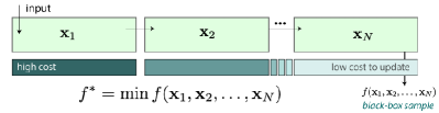
Let denote the variables in the module, and let denote the set of variables across all modules. Our main goal is to propose a cost-efficient algorithm that finds the optimizer for a black-box function,
The function is unknown to us, but when a set of variables are input into the system, this generates a noisy output , where is -sub-Gaussian. To ensure that our model of the cost reflects the modular structure of the system, we make the following assumptions: (i) running the module incurs cost , (ii) a module needs to be run only if variables in some modules earlier than it in the pipeline has been changed from previous iteration. We will also assume that , as any update requires updating variables in the last module, is negligible and equal to . Under the above modeling assumptions, the total cost incurred at iteration is equal to,
| (6) |
where is an indicator that equals to when any variable in modules before the module have been changed from the previous iteration. We refer to the quantity as the movement cost. In our image analysis pipeline experiment (Section 5.2), costs can be thought of as the amount of time or the amount of compute required to re-run a specific module and all of the subsequent modules that follow. In this case, our goal is to perform an end-to-end optimization on the system to maximize the accuracy on a validation set, which can be measured with an f1-score or some other measure of the accuracy of the segmented output.
To trade-off between cost efficiency and functional optimality, we define the movement regret as,
| (7) |
serves as a regularizer which is added to the standard definition of the cumulative regret. In general, the function value and the cost are measured in different units, so should depend on the scales of data.
3.2 Algorithm
This section we provide the descriptions of the steps in the proposed algorithm 1 named Lazy Modular Bayesian Optimization (LaMBO).
Step 1) Modular Structure Embedding Phase.
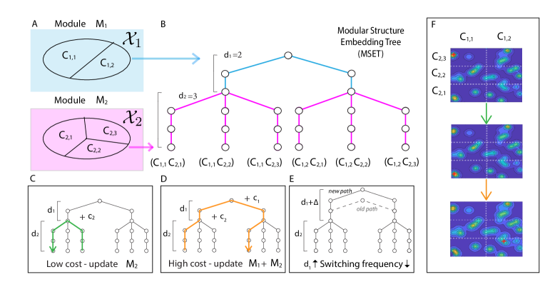
To visualize our algorithmic approach, we point the reader to Figure 2. In the first stage of our optimization procedure, we need to encode the switching costs associated with the system of interest. To do this, we take inspiration from the SMB algorithm described in Section 2.2 to encode the cost to switch variables using a tree-based approach (Figure 2B). We start by linking each arm with a region (subset) of variable space. The regions are flexible and can be partitioned in different ways, but should reflect the modular structure in the system. Thus, we choose to partition the variable space of each module separately. Specifically, defines a partition for the module, where . We require these sets to be disjoint for . Thus, when selecting an arm, we select a joint region of the first modules111We exclude the last module from partitioning procedure since the cost of changing parameters in the last module is the minimum cost per iteration, and can be changed freely at each iteration., i.e., .
Next, we represent the arms in a tree to encode the cost of switching between any two variable subsets. Intuitively, we want to build a tree that encodes the cost of switching between any two sets of hyperparameters (arms) in terms of the shortest path between these two leaves in the tree. Specifically, in Line of Algorithm 1, we call a subroutine ConstructMSET which returns a tree (modular structure embedding tree, MSET), given a partitioning of the variables across all modules and depth parameters , where is the depth of the mth module. The partition and modular specification define the leaves of the tree and the depth parameters control the probability of switching, with higher depth in a module corresponding to lower switching probability (more laziness). In our example ( Figure 2B) , the tree consists of two parts (colored with blue and red) divided by the first forks, the upper portion corresponds to the partition of the first module, while the lower portion corresponds to the partition of the second module. In this case, the depth in the second module is set to 3 to reflect higher relative costs between the two modules and encourage lazy switching behavior.
Step 2) Optimization Phase.
Now the remaining task is to devise a strategy for arm selection and estimate the local optimum within its corresponding variable subset. We propose to use SMB for region (arm) selection, and then use a BO strategy to search within the selected region (Line ). The parameters of SMB and BO are updated at each iteration (Line ). Unfortunately, direct application of BO changes all variables across each iteration, which typically incurs maximum cost. Hence, we propose an alternative lazy strategy: when the same variable subset is selected in an early module, we will use the results from the previous iteration rather than updating the outputs from this lazy module. This means that we do not need to rerun the module and thus can minimize the overall cost. Specifically, let be the arm we’ve selected and be its associated variable region. We propose to search for a block-wise update that minimizes the loss as follows:
| (8) |
where is the first module that has a variable region that differs from the previous iteration , and is a BO acquisition function.
3.3 Empirical construction of MSET
A crucial part of algorithm is the design of the subroutine ConstructMSET, which involves partitioning the variables in each module, and setting the depth parameters (’s). From our experiments, we observe that simple bisection aligned with coordinates yields good partition on many synthetic data and on our neural data. For a MSET with leaves with the partition, LaMBO requires solving local BO optimization problems per iteration. Hence initially, we partition each variable space of module to two subsets only, and abandon subsets when their arm selection probability is below some threshold after consecutive iterations. In our experiments, we always set the threshold to be , where denotes the number of leaves of MSET. After that, we further divide the remaining subsets again to increase the resolution. This procedure could be iterated upon further although we typically do not go beyond two stages of refinement. To avoid trapping in the local optimum, we also refresh the arm-selection probability and update the kernel hyperparameters simultaneously every iterations.
In our implementation, we set the depth parameter to be or when could be estimated in prior. Empirically, we found that the performance is quite robust when for the different cost ratios in both synthetic and real experiments we tested. To avoid accumulating cost too fast in early stages of LaMBO, we record the number of times that variable changes in the first module and dynamically increase the first depth parameters by every iterations when the the number has increased beyond ( of the cycle) during the period. In all experiments, we have found this simple add-on perform on par or better than fixing depth parameters through an entire run.
4 Algorithmic Analysis
In this section, we analyze the performance of Algorithm 1 from two perspectives: 1. Optimization accuracy and 2. Cost efficiency. Our main result, which is stated in Theorem 1, shows that LaMBO achieves sublinear movement regret when the parameters of the input tree are set properly using the cost structure of the system.
Our results are presented in terms of maximum information gain defined below.
Definition 1. Maximum Information Gain. Let be defined in the domain . The observation of at any is given by the model , . For any set , let and denote the set of function values and observations at points in , and denote the Shannon Mutual Information. The Maximum Information Gain is defined by
Analytical bounds on of common kernels are provided in Supp. A.2. To proceed with our analysis, we make the following assumption on the objective function.
Assumption 1. The function is -Lipschitz, non-negative, and has a bounded norm in the reproducing kernel Hilbert space .
Note that our assumption is not too stringent since for any function in a Hilbert space defined above, can be estimated by ; for instance, for exponential kernel since .
4.1 Optimization Accuracy
Our first lemma concerns the optimization capability of LaMBO under a common definition of regret, . Note that we choose to represent it in expectation instead of a probability bound for notational compactness. Conversion to one another is straightforward by common technique like Markov inequality.
Lemma 1.
Ordinary Regret Bound. Suppose the learning rate of the LaMBO is set to be , where is the depth of the MSET, then the expected cumulative regret of LaMBO is:
Remark 1.
By treating modules as arms, a natural comparison is the result of SMB in [Koren et al., 2017b] where . As the arms are represented as leaves of a binary tree with depth , we must have , which shows that the regret bound we have is upper bounded by the result of SMB. The equality holds when the tree is complete. On the other hand, the gap between us could be potentially large. The key to this improvement is by leveraging arm correlation; by using Gaussian surrogate, each sample gives the information of not only the pulled arm itself, but also that of infinitely many others.
4.2 Analysis of Cost Efficiency
Next, we analyze the cost incurred by adopting LaMBO. The following lemma shows that LaMBO is capable of accumulating sublinear cost. The result also gives an explicit recipe of choosing parameters of MSET from theory. Below we provide a sketch of the achievable rate and defer the detailed forms of parameters to Supp. A.1.
Lemma 2.
Cumulative Switching Cost. For sufficiently large , there exists depth parameters of the MSET such that LaMBO accumulates movement cost
Remark 2.
A striking implication of Lemma 2 is that even with nonconstant cost , the cumulative cost could still be sublinear as long as .
Finally combining the above two lemmas leads to our concluding theorem, which shows that a simple partition strategy, along with proper selection of the depth parameters , gives sublinear movement regret defined in (7). Without additional information about how to partition each module, the simplest way to partition the space is uniformly. Hence in the analysis we adopt an uniform partition strategy characterized by , where denotes the Euclidean diameter of the partitioned subset .
Now we present a sketch of our main theoretical result where a proof and detailed constants could be found in Supp. A.1.
Theorem 1.
Movement Regret Bound. For , let denote the dimension of . Suppose for all , , we set , . The MSET has uniform partition of each with diameters , where the depth parameters are chosen according to Lemma 2, and UCB acquisition function is used. Then LaMBO achieves the expected movement regret
Remark 3.
Comparisons to moving bandit algorithm: A black-box optimization strategy blind to switch cost usually has , and thus obtain a linear movement regret . For switch-cost-aware alternatives, the closest result on moving regret is Theorem in [Koren et al., 2017b]. However, their result relies on the Lispchitz property of the movement metric, which does not hold in our setting as the cost from changing variables in modules is not even continuous. By leveraging arms correlation with BO and adapting a lazy arm selection strategy, we extend their result by achieving a sublinear rate.
5 Experiments
In this section, we start by testing LaMBO on benchmark synthetic functions used in other studies [Vellanki et al., 2017, Kirschner et al., 2019]. Following this, we apply LaMBO to tune a multi-stage neuroimaging pipeline that reconstructs 3D images from segmented 2D images.
Experimental setup.
For simplicity, we used the squared exponential kernel and initialized it using random samples before starting the inference procedure. In our experiments, the functions are normalized by their maximized absolute value for clear comparisons, the regularization parameter is fixed to , the UCB parameter is set each iteration as , and the learning rate is set to . The sampling noise is assumed to be independent Gaussian with standard deviation . For construction of MSET, we test on the simplest case where and partition the variable space in each module into 2 sets aligned with a random coordinate. Some practical and detailed discussions on the hyperparameter choices and partition strategies are deferred to Supp. B. The curves on synthetic data and real data were computed by averaging across and simulations, respectively. We compare LaMBO with common baselines GP-UCB [Srinivas et al., 2010], GP-EI [Močkus, 1975], Max-value entropy search [Wang and Jegelka, 2017], random sampling, and three cost-aware strategies: EIpu [Snoek et al., 2012], CA-MOBO [Abdolshah et al., 2019], and CArBO [Lee et al., 2020]. To adapt the cost-aware strategies to our setting, we update the cost function at each iteration to be to the switching cost defined in Eqn. (6) in Section 3.
5.1 Experiments on synthetic functions
For synthetic benchmarks, we selected a number of common functions used to test algorithms in the literature. However, unlike our real data examples that have clear modular structure due to the different sets of operations performed at different stages, the variables in synthetic test functions do not readily admit a modular structure. Thus to simulate a -module or -module scenario, we divide the variables in each function into different groups to create effective modules.
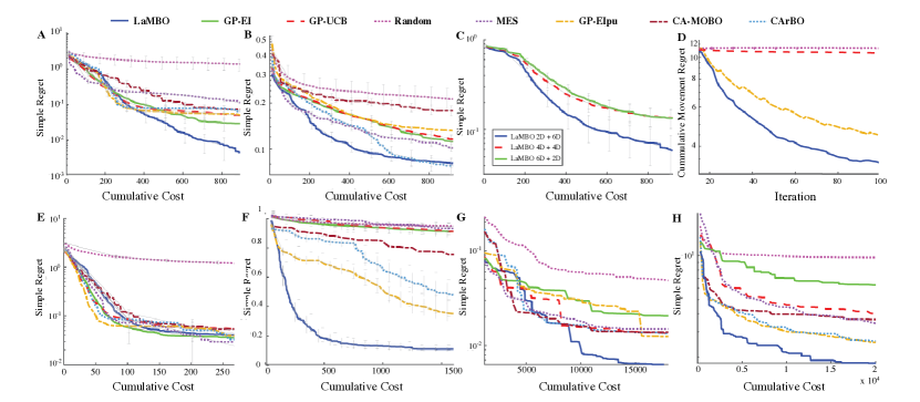
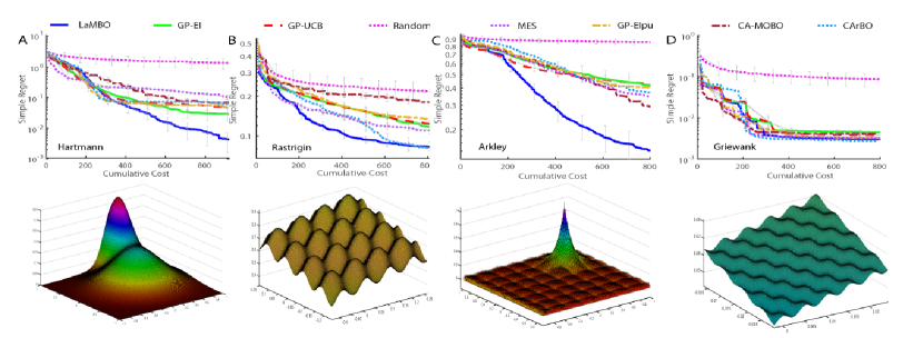
In Figure 3 (A-D), we compare the methods on synthetic functions in a two-module setting with a cost ratio of to . In (A-B), we show the results for two different synthetic functions Hartmann and Rastrigin, respectively (more experiments on synthetic functions could be found in Supp. E). In (C), we study the impact of splitting variables into sets of different dimensions with function Ackley 8D, a synthetic function with a sharp global optimum surrounded with multiple local ones. The result suggests LaMBO is stable among different variable configurations in modules. Under the same setting as in (A), we verify our regret analysis by plotting the cumulative movement regret curve in (D), and study the performance of the different approaches when the cost is . The former shows that LaMBO minimizes the averaged movement regret of (7) better than cost-aware and unaware baselines. The later shows that LaMBO performs better when the cost ratio between modules is large while on par with alternative when the ratio is . (F) explores the -module setting of Ackley 8D (), with the cost . In this case, we found that it performs even better than its -module counterpart in Figure reffig:synsupp, suggesting LaMBO’s applicability in pipeline with many modules.
Overall, we find that LaMBO outperforms other approaches and really shines when the cost of earlier modules is much larger (as seen in (A) vs. (E)). When we track the optimization trajectory, we observe that LaMBO performs similarly to other methods early on, but with further iterations, LaMBO starts to outperform the alternatives. This could be explained by inaccurate estimation of the function at early stages, and the fact that aggressive input changes could outperform the more conservative or lazy strategy used in LaMBO. However, as more samples are gathered, LaMBO demonstrates more power in terms of its cost efficiency by being lazy in variable switching.
5.2 Application to a multi-stage neuroimaging pipeline
Segmentation and identification of neural structures of interest (e.g., cell bodies, axons, or vasculature) is an important problem in connectomics and other applications of brain mapping [Helmstaedter et al., 2013, Oh et al., 2014, Dyer et al., 2017]. However, when dealing with large datasets, transfer can be challenging, and thus workflows must be re-optimized for each new dataset [Johnson et al., 2020]. Here, we consider the optimization of a relatively common three-stage pipeline, consisting of a pre-processing (image enhancement via denoising and contrast normalization), semantic segmentation for pixel-level prediction (via an U-net architecture), and a post-processing operation (to reconstruct a 3D volume). For comparison, we also consider a simplified pipeline without the pre-processing. To optimize this pipeline, we use a publicly available X-ray microCT dataset [Prasad et al., 2020] to set up the experiments in both a two-module (no pre-processing) and full three-module version of the pipeline.
In the first module, a pre-processing operation is performed where we tune a contrast parameter and denoising parameter. In the second module we train an U-Net, where in this case we tune the learning rate and batch size. The third module is in charge of post-processing and generates 3D reconstructions from the U-Net output; the hyperparameters in this module include a label purity score, cell opening size, and a shape parameter to determine whether uncertain components are either cells or blood vessels. Details of search space for each module are described in Supp. 5.2). The cost of the experiment is the aggregate recorded clock time for generating an output after changing a variable in a specific module. To test LaMBO on the problem, we gathered an offline data set consisting of different hyperparameters obtained by exhaustive search.
In the two-module case (Figure 3G), we observe a transition effect; when enough cost has been spent, LaMBO starts to increase its gap in performance over other methods. In the three-module case (Figure 3H) the advantage is even more pronounced, where the transition happens earlier. Quantitatively it shows that to get close to the optimum (within 5%), LaMBO can achieve this result in only 25% of the time required by the best alternative approach (1.4 vs. 5.6 hours).
6 Discussion
This paper addresses a real-world problem of system optimization that is encountered in a variety of scientific disciplines. Increasingly, as we expand the size of datasets in different domains, we need automated solutions to quickly apply advanced machine learning systems to new datasets and re-optimize systems in an end-to-end manner. To tackle this problem, we introduced a new algorithm for Bayesian optimization that leverages known modular structure in an otherwise black-box system to minimize the overall cost required for global optimization. We showed how to leverage structure in such systems by incorporating a lazy switching strategy with Bayesian optimization. In the future, we would like to generalize our method to the case where both the function and switching costs are unknown, and extend to more complex cost hierarchies.
Acknowledgements
This work was supported by the NIH award 1R24MH114799-01 and awards IIS-1755871 and CCF-1740776 from the NSF.
References
- Abdolshah et al. [2019] Majid Abdolshah, Alistair Shilton, Santu Rana, Sunil Gupta, and Svetha Venkatesh. Cost-aware multi-objective bayesian optimisation. arXiv preprint arXiv:1909.03600, 2019.
- Abraham et al. [2014] Alexandre Abraham, Fabian Pedregosa, Michael Eickenberg, Philippe Gervais, Andreas Mueller, Jean Kossaifi, Alexandre Gramfort, Bertrand Thirion, and Gaël Varoquaux. Machine learning for neuroimaging with scikit-learn. Frontiers in neuroinformatics, 8:14, 2014.
- Alon et al. [2015] Noga Alon, Nicolo Cesa-Bianchi, Ofer Dekel, and Tomer Koren. Online learning with feedback graphs: Beyond bandits. In Annual Conference on Learning Theory, volume 40. Microtome Publishing, 2015.
- Auer et al. [2002] Peter Auer, Nicolo Cesa-Bianchi, and Paul Fischer. Finite-time analysis of the multiarmed bandit problem. Machine learning, 47(2-3):235–256, 2002.
- Azar et al. [2014] Mohammad Gheshlaghi Azar, Alessandro Lazaric, and Emma Brunskill. Online stochastic optimization under correlated bandit feedback. In ICML, pages 1557–1565, 2014.
- Bergstra et al. [2011] James Bergstra, Rémi Bardenet, Yoshua Bengio, and Balázs Kégl. Algorithms for hyper-parameter optimization. In Proceedings of the 24th International Conference on Neural Information Processing Systems, NIPS’11, page 2546–2554, Red Hook, NY, USA, 2011. Curran Associates Inc. ISBN 9781618395993.
- Berkenkamp et al. [2016] Felix Berkenkamp, Angela P Schoellig, and Andreas Krause. Safe controller optimization for quadrotors with gaussian processes. In 2016 IEEE International Conference on Robotics and Automation (ICRA), pages 491–496. IEEE, 2016.
- Buades et al. [2011] Antoni Buades, Bartomeu Coll, and Jean-Michel Morel. Non-local means denoising. Image Processing On Line, 1:208–212, 2011.
- Chowdhury and Gopalan [2017] Sayak Ray Chowdhury and Aditya Gopalan. On kernelized multi-armed bandits. In Proceedings of the 34th International Conference on Machine Learning - Volume 70, ICML’17, pages 844–853. JMLR.org, 2017. URL http://dl.acm.org/citation.cfm?id=3305381.3305469.
- Davis-Turak et al. [2017] Jeremy Davis-Turak, Sean M Courtney, E Starr Hazard, W Bailey Glen Jr, Willian A da Silveira, Timothy Wesselman, Larry P Harbin, Bethany J Wolf, Dongjun Chung, and Gary Hardiman. Genomics pipelines and data integration: challenges and opportunities in the research setting. Expert review of molecular diagnostics, 17(3):225–237, 2017.
- Dekel et al. [2014] Ofer Dekel, Jian Ding, Tomer Koren, and Yuval Peres. Bandits with switching costs: T 2/3 regret. In Proceedings of the forty-sixth annual ACM symposium on Theory of computing, pages 459–467, 2014.
- Dyer et al. [2017] Eva L Dyer, William Gray Roncal, Judy A Prasad, Hugo L Fernandes, Doga Gürsoy, Vincent De Andrade, Kamel Fezzaa, Xianghui Xiao, Joshua T Vogelstein, Chris Jacobsen, et al. Quantifying mesoscale neuroanatomy using x-ray microtomography. Eneuro, 4(5), 2017.
- Feldman et al. [2016] Michal Feldman, Tomer Koren, Roi Livni, Yishay Mansour, and Aviv Zohar. Online pricing with strategic and patient buyers. In Advances in Neural Information Processing Systems, pages 3864–3872, 2016.
- Frazier [2018] Peter I Frazier. A tutorial on bayesian optimization. arXiv preprint arXiv:1807.02811, 2018.
- Garnett et al. [2010] R. Garnett, M. A. Osborne, and S. J. Roberts. Bayesian optimization for sensor set selection. In Proceedings of the 9th ACM/IEEE International Conference on Information Processing in Sensor Networks, IPSN ’10, page 209–219, New York, NY, USA, 2010. Association for Computing Machinery. ISBN 9781605589886. 10.1145/1791212.1791238. URL https://doi.org/10.1145/1791212.1791238.
- González et al. [2016] Javier González, Zhenwen Dai, Philipp Hennig, and Neil Lawrence. Batch bayesian optimization via local penalization. In Artificial intelligence and statistics, pages 648–657, 2016.
- Helmstaedter et al. [2013] Moritz Helmstaedter, Kevin L Briggman, Srinivas C Turaga, Viren Jain, H Sebastian Seung, and Winfried Denk. Connectomic reconstruction of the inner plexiform layer in the mouse retina. Nature, 500(7461):168–174, 2013.
- Johnson et al. [2019] Erik C Johnson, Miller Wilt, Luis M Rodriguez, Raphael Norman-Tenazas, Corban Rivera, Nathan Drenkow, Dean Kleissas, Theodore J LaGrow, Hannah Cowley, Joseph Downs, et al. Toward a reproducible, scalable framework for processing large neuroimaging datasets. BioRxiv, page 615161, 2019.
- Johnson et al. [2020] Erik C Johnson, Miller Wilt, Luis M Rodriguez, Raphael Norman-Tenazas, Corban Rivera, Nathan Drenkow, Dean Kleissas, Theodore J LaGrow, Hannah P Cowley, Joseph Downs, et al. Toward a scalable framework for reproducible processing of volumetric, nanoscale neuroimaging datasets. GigaScience, 9(12):giaa147, 2020.
- Kalai and Vempala [2005] Adam Kalai and Santosh Vempala. Efficient algorithms for online decision problems. Journal of Computer and System Sciences, 71(3):291–307, 2005.
- Kandasamy et al. [2016] Kirthevasan Kandasamy, Gautam Dasarathy, Junier B Oliva, Jeff Schneider, and Barnabás Póczos. Gaussian process bandit optimisation with multi-fidelity evaluations. In Advances in Neural Information Processing Systems, pages 992–1000, 2016.
- Kandasamy et al. [2017] Kirthevasan Kandasamy, Gautam Dasarathy, Jeff Schneider, and Barnabás Póczos. Multi-fidelity bayesian optimisation with continuous approximations. In Proceedings of the 34th International Conference on Machine Learning-Volume 70, pages 1799–1808. JMLR. org, 2017.
- Kathuria et al. [2016] Tarun Kathuria, Amit Deshpande, and Pushmeet Kohli. Batched gaussian process bandit optimization via determinantal point processes. In Advances in Neural Information Processing Systems, pages 4206–4214, 2016.
- Kirschner et al. [2019] Johannes Kirschner, Mojmír Mutnỳ, Nicole Hiller, Rasmus Ischebeck, and Andreas Krause. Adaptive and safe bayesian optimization in high dimensions via one-dimensional subspaces. arXiv preprint arXiv:1902.03229, 2019.
- Koren et al. [2017a] Tomer Koren, Roi Livni, and Yishay Mansour. Multi-armed bandits with metric movement costs. In I. Guyon, U. V. Luxburg, S. Bengio, H. Wallach, R. Fergus, S. Vishwanathan, and R. Garnett, editors, Advances in Neural Information Processing Systems 30, pages 4119–4128. Curran Associates, Inc., 2017a.
- Koren et al. [2017b] Tomer Koren, Roi Livni, and Yishay Mansour. Bandits with movement costs and adaptive pricing. In Satyen Kale and Ohad Shamir, editors, Proceedings of the 2017 Conference on Learning Theory, volume 65 of Proceedings of Machine Learning Research, pages 1242–1268, Amsterdam, Netherlands, 07–10 Jul 2017b. PMLR. URL http://proceedings.mlr.press/v65/koren17a.html.
- Lam and Willcox [2017] Remi Lam and Karen Willcox. Lookahead bayesian optimization with inequality constraints. In Advances in Neural Information Processing Systems, pages 1890–1900, 2017.
- Lam et al. [2016] Remi Lam, Karen Willcox, and David H Wolpert. Bayesian optimization with a finite budget: An approximate dynamic programming approach. In Advances in Neural Information Processing Systems, pages 883–891, 2016.
- Lee et al. [2020] Eric Hans Lee, Valerio Perrone, Cedric Archambeau, and Matthias Seeger. Cost-aware bayesian optimization, 2020.
- Lee et al. [2019] Kisuk Lee, Nicholas Turner, Thomas Macrina, Jingpeng Wu, Ran Lu, and H Sebastian Seung. Convolutional nets for reconstructing neural circuits from brain images acquired by serial section electron microscopy. Current opinion in neurobiology, 55:188–198, 2019.
- McLeod et al. [2017] Mark McLeod, Michael A Osborne, and Stephen J Roberts. Practical bayesian optimization for variable cost objectives. arXiv preprint arXiv:1703.04335, 2017.
- Mockus [1982] J. Mockus. The bayesian approach to global optimization. In R. F. Drenick and F. Kozin, editors, System Modeling and Optimization, pages 473–481, Berlin, Heidelberg, 1982. Springer Berlin Heidelberg. ISBN 978-3-540-39459-4.
- Močkus [1975] Jonas Močkus. On bayesian methods for seeking the extremum. In Optimization techniques IFIP technical conference, pages 400–404. Springer, 1975.
- Mockus et al. [1978] Jonas Mockus, Vytautas Tiesis, and Antanas Zilinskas. The application of bayesian methods for seeking the extremum. Towards global optimization, 2(117-129):2, 1978.
- Oh et al. [2014] Seung Wook Oh, Julie A Harris, Lydia Ng, Brent Winslow, Nicholas Cain, Stefan Mihalas, Quanxin Wang, Chris Lau, Leonard Kuan, Alex M Henry, et al. A mesoscale connectome of the mouse brain. Nature, 508(7495):207–214, 2014.
- Poloczek et al. [2017] Matthias Poloczek, Jialei Wang, and Peter Frazier. Multi-information source optimization. In Advances in Neural Information Processing Systems, pages 4288–4298, 2017.
- Prasad et al. [2020] JA Prasad, AH Balwani, E Johnson, JD Miano, V Sampathkumar, V de Andrade, M Du, R Vescovi, C Jacobsen, D Gursoy, N Kasthuri, and EL Dyer. A three-dimensional thalamocortical dataset for characterizing brain heterogeneity. under review in Nature Scientific Data, 2020.
- Rasmussen [2003] Carl Edward Rasmussen. Gaussian processes in machine learning. In Summer School on Machine Learning, pages 63–71. Springer, 2003.
- Snoek et al. [2012] Jasper Snoek, Hugo Larochelle, and Ryan P Adams. Practical bayesian optimization of machine learning algorithms. In Advances in neural information processing systems, pages 2951–2959, 2012.
- Srinivas et al. [2010] Niranjan Srinivas, Andreas Krause, Sham Kakade, and Matthias Seeger. Gaussian process optimization in the bandit setting: No regret and experimental design. In Proceedings of the 27th International Conference on International Conference on Machine Learning, ICML’10, pages 1015–1022, USA, 2010. Omnipress. ISBN 978-1-60558-907-7. URL http://dl.acm.org/citation.cfm?id=3104322.3104451.
- [41] S. Surjanovic and D. Bingham. Virtual library of simulation experiments: Test functions and datasets. Retrieved February 3, 2020, from http://www.sfu.ca/~ssurjano.
- Vellanki et al. [2017] Pratibha Vellanki, Santu Rana, Sunil Gupta, David Rubin, Alessandra Sutti, Thomas Dorin, Murray Height, Paul Sanders, and Svetha Venkatesh. Process-constrained batch bayesian optimisation. In Advances in Neural Information Processing Systems, pages 3414–3423, 2017.
- Wang and Jegelka [2017] Zi Wang and Stefanie Jegelka. Max-value entropy search for efficient bayesian optimization. In Proceedings of the 34th International Conference on Machine Learning-Volume 70, pages 3627–3635. JMLR. org, 2017.
- Wang et al. [2014] Ziyu Wang, Babak Shakibi, Lin Jin, and Nando Freitas. Bayesian multi-scale optimistic optimization. In Artificial Intelligence and Statistics, pages 1005–1014. PMLR, 2014.
- Wu et al. [2020] Jian Wu, Saul Toscano-Palmerin, Peter I Frazier, and Andrew Gordon Wilson. Practical multi-fidelity bayesian optimization for hyperparameter tuning. In Uncertainty in Artificial Intelligence, pages 788–798. PMLR, 2020.
Supplementary Materials
Appendix A Technical Preliminaries and Proofs
A.1 Proofs of Theoretical Results
Lemma 3.
(Theorem of [Chowdhury and Gopalan, 2017]). Let be a function lying in the RKHS of kernel such that with input dimension . Assume the process of observation noise is -sub-gaussian. Then setting
we have the following holds with probability at least ,
where are given by the formula
Lemma 4.
(Lemma 4 of [Chowdhury and Gopalan, 2017]). Suppose we sample the objective function at then the sum of standard deviations is bounded by,
Our first goal is to prove Lemma 1.
Lemma 1.
Suppose the learning rate of the LaMBO is set to be , where is the depth of the MSET, then the expected cumulative regret of LaMBO is:
Remark 4.
We can compare the result with SMB in [Koren et al., 2017b] where . Note that ours is a lower bound of it as . They could potentially have a large gap between them in terms of order. This performance improvement is due to our loss estimator adapted to arm correlation, whereas [Koren et al., 2017b] considers the pure bandit information.
Lemma 5.
For any sequence of , denote to be the solution of and assume for some constant , then there exists an such that LaMBO has the property
For the proof of 5 we follow the path in [Koren et al., 2017a]. Before we start the proof of Lemma 5, we will need Lemma 6, 7, 8, and 9.
Lemma 6.
| (9) |
In particular, if then for all .
Proof.
The last statement is trivial from definition. We will prove Eq. (6) by induction on . Since by Eq. (8) and the UCB is upper bounded by , the statement holds for . Now assume it holds for . Then firstly,
Secondly, applying Jensen’s inequality, we have
where the second inequality is followed by the induction assumption. Therefore the proof is complete by mathematical induction. ∎
Lemma 7.
For all and the followings hold:
-
•
For all we have
(10) -
•
With probability at least , we have that .
Proof.
The proof of the second property is identical to Lemma 8 in [Koren et al., 2017a] and is thus omitted . Now we prove the first property. Note that we only need to prove
| (11) |
We will again use the mathematical induction to prove the above statement. The initial case holds trivially. Now assume the statement is true for . Then for ,
where the last equality follows from the induction assumption. On the other hand,
where the last equality follows from the independence between and . Hence we have
| (12) |
Now if . Let be the subtree such that then by the tower rule for expectation we have
Therefore,
| (13) |
By (12), (13) now holds for every possible value of , so we must have
which completes the proof by induction. ∎
Lemma 8.
For all , we have .
Proof.
Lemma 9.
[Alon et al., 2015]. Let and be real vectors such that then a sequence of probability vectors defined by and for all ,
have the property that
for any .
Now we are ready to prove Lemma 5.
Proof.
Next we prove Lemma 2 in the main text.
Lemma 2.
For sufficient large , suppose for that the parameters of an MSET are chosen recursively,
| (17) |
Then LaMBO results in cumulative costs
| (18) |
Proof.
The proof follows by showing firstly that the movement cost is dominated by a HST metric, and secondly that under the tree metric the cumulative cost is bounded by the quantity in the lemma. To define the HST metric formally, let us introduce the following terminology in accordance to [Koren et al., 2017b]. Given , be nodes in the MSET , let LCA() be their least common ancestor node. Then the scaled HST metric is defined as follows:
| (19) |
Under this metric, the cost incurred from changing variables in the module is
Then the condition of dominance over the original cost is, for ,
Rearrangements of these linear inequalities yield the solution for to as
| (20) |
Under the condition in Eq. (A.1), the cost incurred from the HST metric Eq. (19) is larger than our original cost. Hence, an upper bound for the cost incurred from the metric will also bound our cumulative cost.
Now we bound the cumulative cost under this HST metric. Observe and belongs to the same subtree on level of the tree with probability at least , therefore we have
| (21) |
On the other hand, the condition of admits a non-negative solution of for sufficient large . This condition implies an upper bound on . Finally, combining this upper bound of with Eq. (A.1) completes the proof. ∎
Now we are in the last stage of proving Theorem 1.
Theorem 1.
For , let denote the dimension of and suppose for all , we set , , and we have an MSET with a uniform partition of each with diameters , where the depth parameters follows from Lemma 2. Then LaMBO achieves the expected movement regret
Proof.
We first bound the ordinary regret. Choose . Then, with probability , we have
| (22) |
where (a) follows from Lemma 3 and (b) from the fact that for some and that is -Lipschitz.
Note that when the above inequality fails it only contributes to cumulative regret in expectation by , so we can ignore this term in later calculation.
Now, taking expectation on both sides of Eq. (A.1) yields
where (c) follows from Lemma 4, (d) from that , and (e) from Lemma 5 where for .
On the other hand, the cumulative movement cost by Lemma 2 is
| (23) |
From Eq. (23), we plug in , and .
Then, we have
and
which completes the proof. ∎
A.2 Bounds on the maximum mutual information for common kernels
The following lists known bounds of the maximum mutual information for common kernels [Srinivas et al., 2010]:
-
•
, for linear kernel.
-
•
, for Squared Exponential kernel.
-
•
for Matérn kernels with ,
where is the dimension of input space.
Appendix B Practical considerations and implementation details
B.1 Details on model selection
Below we detail the extensions we use in the experiments to improve the algorithm’s performance.
Restart with Epochs: A plausible strategy is to refresh the arm-selection probability every iterations to escape from local optimum. In our implementation we choose as the default value.
Adaptive Resolution Increase: In experiments, a simple extension allows LaMBO to discard the arms that have probability of selection being less than a threshold ( in our implementation), and partition each remaining subset into subsets. We found that combining this with restart can accelerate the optimization in many cases.
Update of Kernel: We choose RBF kernel and Mátern class. As commonly found in practice, we update our kernel hyperparameters every iterations based on the maximum likelihood estimation.
Aggressive learning rate: Our experiments show that constant learning rate usually outperforms the rate suggested by the theory.
B.2 Further design of MSET and partition strategies
Construction of MSET:
A crucial part of algorithm is in the construction of the MSET, which involves partitioning the variables in each module, and setting the depth parameters (’s). For a MSET with leaves to choose from, LaMBO requires solving local BO optimization problems per iteration. Hence initially, we partition each variable space of module to two subsets only, and abandon subsets when their arm selection probability is below some threshold. In our experiments, we always set it to be , where denotes the number of leaves of MSET. After that, we further divide the remaining subsets again to increase the resolution. This procedure could be iterated upon further although we typically do not go beyond two stages of refinement.
In our implementation, we set the depth parameter to be or when could be estimated in prior. Empirically, we found that the performance is quite robust when for the different cost ratios in both synthetic and real experiments we tested. To avoid accumulating cost too fast in early stages of LaMBO, we record the number of times that variable changes in the first module and dynamically increase the first depth parameters by every iterations when the the number has increased beyond ( of the cycle) during the period. In all experiements, we have found this simple add-on perform on par or better than fixing depth parameters through an entire run.
Partitioning method:
Although LaMBO achieves theoretical guarantees with a uniform partition, such a partition does not fully leverage the structure of the function. For this reason, the computational complexity can be very large for high-dimensional problems. On the other hand, we observe from our experiments that simple bisection aligned with coordinates yields good performance on many synthetic data and on our neural data. To further improve the performance, we adopt the multi-scale optimization strategy [Wang et al., 2014, Azar et al., 2014], which adaptively increases the partition resolution through iterations. Practically it has often leads to more computational savings, which involves partitioning more finely in regions that have high rewards. A simple version of this strategy is also employed in our experiments where regions are discarded with probability of selection being below some threshold (typically ) and the remaining regions are further partitioned with increasing resolution. Another remedy is to use domain specific information to help restrict the search space or define the hierarchy in the MSET. The generality of the MSET makes it possible to use expert or prior knowledge to constrain switching between specific sets of variables that may be implausible. For instance, in our study of application in neuroscience, there are certain combinations of parameters that would violate certain size constraints related to the underlying biology that could be incorporated into the design of the MSET.
Appendix C Further details on the neuroimaging experiments
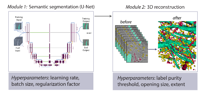
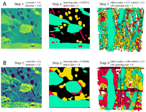
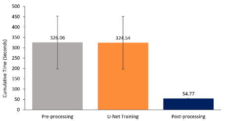
Figure S1 illustrates the scheme of our brain-imaging experiment without pre-processing. In this brain mapping pipeline, we varied the U-Net training hyperparameters and the 3D reconstruction post-processing hyperparameters. In the first module (U-Net training), we optimized the learning rate and batch size for the U-Net. In the second module, we applied post-processing operations to the U-Net output 3D reconstructions, including label purity , cell opening size , and a shape parameter (extent) to determine whether uncertain components are either cells or blood vessels .
We also performed a 3-module experiment by adding a pre-processing before U-Net training. We varied the pre-processing hyperparameters, U-Net training hyperparameters, and 3D reconstruction post-processing hyperparameters. In the pre-processing, we used a contrast parameter and denoising parameter (regularization strength in Non-Local Means [Buades et al., 2011]), and in the second module (U-Net training), we varied the learning rate and batch size . During the third module (post-processing of 3D reconstructions), we varied label purity , cell opening size , and extent . In our experiments, we define the cost to be the aggregate recorded clock time for generating an output after changing a variable in a specific module (see Figure S2, right). To test LaMBO on the problem, we gathered a data set consisting of combinations of hyperparameters by exhaustive search.
Appendix D Pseudo-code for the Slowing Moving Bandit Algorithm
For completeness, we include a pseudo-code for slowly moving bandit algorithm below.
Appendix E Further Experiments on Synthetic Functions
The synthetic functions used in the experiment are taken from [Surjanovic and Bingham, ] and [Kandasamy et al., 2016]. We use linear transformation to normalize all the function to the range .
We compare LaMBO with other BO algorithms on four synthetic functions, (A) Hartmann 6D, (B) Rastrigin 6D, (C) Ackley 8D, and (D) Griewank 6D. The plots on the top shows the regret performance, the plots on the button show their surface. We observe when objective have multiple local optimum comparable with the global one, LaMBO has comparable performance with the alternative. However, LaMBO performs significantly better than the baselines when the objective has a sharper global optimum. Unlike deterministic decision rule proposed in the alternatives, LaMBO has randomized decision rule and does not rely on the GP regression alone, which allows it to have more incentive for exploration.
Hartmann 6D function:
The function is , where
and the domain is .
Ackley 8D function:
where the domain is .
Rastrigin 6D function:
where the domain is .
Griewank 6D function:
where the domain is .