An Improved LSHADE-RSP Algorithm with the Cauchy Perturbation: iLSHADE-RSP
Abstract
A new method for improving the optimization performance of a state-of-the-art differential evolution (DE) variant is proposed in this paper. The technique can increase the exploration by adopting the long-tailed property of the Cauchy distribution, which helps the algorithm to generate a trial vector with great diversity. Compared to the previous approaches, the proposed approach perturbs a target vector instead of a mutant vector based on a jumping rate. We applied the proposed approach to LSHADE-RSP ranked second place in the CEC 2018 competition on single objective real-valued optimization. A set of 30 different and difficult optimization problems is used to evaluate the optimization performance of the improved LSHADE-RSP. Our experimental results verify that the improved LSHADE-RSP significantly outperformed not only its predecessor LSHADE-RSP but also several cutting-edge DE variants in terms of convergence speed and solution accuracy.
keywords:
Artificial Intelligence , Evolutionary Algorithm , Differential Evolution , Mathematical Optimization1 Introduction
A population-based metaheuristic optimization method called evolutionary algorithms (EAs) is designed based on Darwin’s theory of natural selection. EAs generate a set of initial candidate solutions and update them iteratively with artificially designed evolutionary operators. As compared to traditional search algorithms, EAs are global, robust, and can be applied to any problem.
It is important to establish a balance between exploration and exploitation to improve the optimization performance of EAs. Matej et al. [1] stated that “Exploration is the process of visiting entirely new regions of a search space, whilst exploitation is the process of visiting those regions of a search space within the neighborhood of previously visited points.” If an EA has too strong exploration, it might not be beneficial from existing candidate solutions [2]. On the other hand, if an EA has too strong exploitation, the probability of finding an optimal solution might be decreased [2]. Many researchers have investigated a number of approaches for balancing the two cornerstones [1].
Differential evolution (DE) proposed by Storn and Price [3, 4] is one of the most successful EAs to deal with mathematical optimization. DE distributes its candidate solutions over the search boundaries of an optimization problem and updates them iteratively with vector difference based evolutionary operators. DE has two main advantages over other EAs: 1) it has a simple structure and a few control parameters, and 2) the effectiveness of DE has been demonstrated on various real-world problems [5, 6]. Among numerous DE variants, L-SHADE variants [7, 8, 9, 10, 11, 12, 13, 14, 15, 16, 17, 18] frequently perform very well on various optimization problems. LSHADE-RSP [17] was recently proposed and ranked second place in the CEC 2018 competition on single objective real-valued optimization.
Although LSHADE-RSP has shown excellent performance, it has the following problem: LSHADE-RSP uses a rank-based selective pressure scheme, which increases the greediness and boosts the convergence speed. However, it may cause premature convergence in which all the candidate solutions fall into the local optimum of an optimization problem and cannot escape from there [19, 20, 21, 22]. Although LSHADE-RSP uses a setting for increasing the number of best individuals in an effort to mitigate the problem, it may not be sufficient. In other words, LSHADE-RSP may fail to achieve exploration and exploitation.
In this paper, we proposed a new method for improving the optimization performance of LSHADE-RSP. The technique perturbs a target vector with the Cauchy distribution based on a jumping rate, which helps the algorithm to generate a trial vector with great diversity. Therefore, the technique can increase the probability of finding an optimal solution by adopting the long-tailed property of the Cauchy distribution. In the literature of DE, some researchers have demonstrated the effectiveness of using the Cauchy distribution in the phase of the recombination [23, 24, 25, 26, 27]. The novelty of the proposed approach lies in the perturbation of a target vector instead of a mutant vector. We named the combination of LSHADE-RSP and the proposed approach as iLSHADE-RSP.
We carried out experiments to evaluate the optimization performance of the proposed algorithm on the CEC 2017 test suite [28]. Our experimental results verify that the proposed algorithm significantly outperformed not only its predecessor LSHADE-RSP but also several state-of-the-art DE variants in terms of convergence speed and solution accuracy.
The rest of this paper is organized as follows: We introduce the background of this paper in Section 2. In Section 3, we review the relevant literature to know, especially for L-SHADE variants. In Section 4, the details of the proposed algorithm is explained. We describe the experimental setup in Section 5. We present the experimental results and discussion in Section 6. Finally, we conclude this paper in Section 7.
2 Background
2.1 Differential Evolution
Since it was introduced, DE [3, 4] has received much attention because of simplicity and applicability. At the beginning of an optimization process, DE generates a set of initial candidate solutions as follows.
| (1) |
where denotes a population at generation . Each candidate solution denoted by is a -dimensional vector. DE updates the candidate solutions iteratively with vector difference based evolutionary operators, such as mutation, crossover, and selection, to search for the global optimum of an optimization problem. The mutation and crossover operators create a set of offspring, and the selection operator creates a population for the next generation by comparing the fitness value of a candidate solution and that of its corresponding offspring. DE returns the current best solution when it reaches the maximum number of generations or function evaluations .
2.1.1 Initialization
At the beginning of an optimization process, DE distributes its candidate solutions over the search boundaries of an optimization problem with the initialization operator. Each candidate solution is initialized as follows.
| (2) |
where and denote the lower and upper search boundaries of an optimization problem, respectively. Also, denotes a uniformly distributed random number between .
2.1.2 Mutation
A mutant vector is created in the mutation operator. The six frequently used classical mutation strategies are listed as follows.
-
1.
DE/rand/1:
-
2.
DE/rand/2:
-
3.
DE/best/1:
-
4.
DE/best/2:
-
5.
DE/current-to-best/1:
-
6.
DE/current-to-rand/1:
where , , , , denote mutually different random indices within , which are also different from . Moreover, denotes the current best candidate solution. Furthermore, denotes a scaling factor, and denotes a uniformly distributed random number between .
2.1.3 Crossover
A trial vector is created in the crossover operator. The binomial crossover frequently used creates a trial vector as follows.
| (3) |
where denotes a random index within . Also, denotes a crossover rate. The exponential crossover creates a trial vector as follows.
| (4) |
where denotes a random index within , and denotes the number of elements, which can be calculated as follows.
DO { }
WHILE ( AND )
Also, denotes the modulo of .
2.1.4 Selection
DE creates a population for the next generation with the selection operator. The selection operator compares the fitness value of a candidate solution () and that of its corresponding offspring () and picks the better one in terms of solution accuracy as follows.
| (5) |
where denotes an optimization problem to be minimized.
2.2 Analysis of Cauchy Distribution
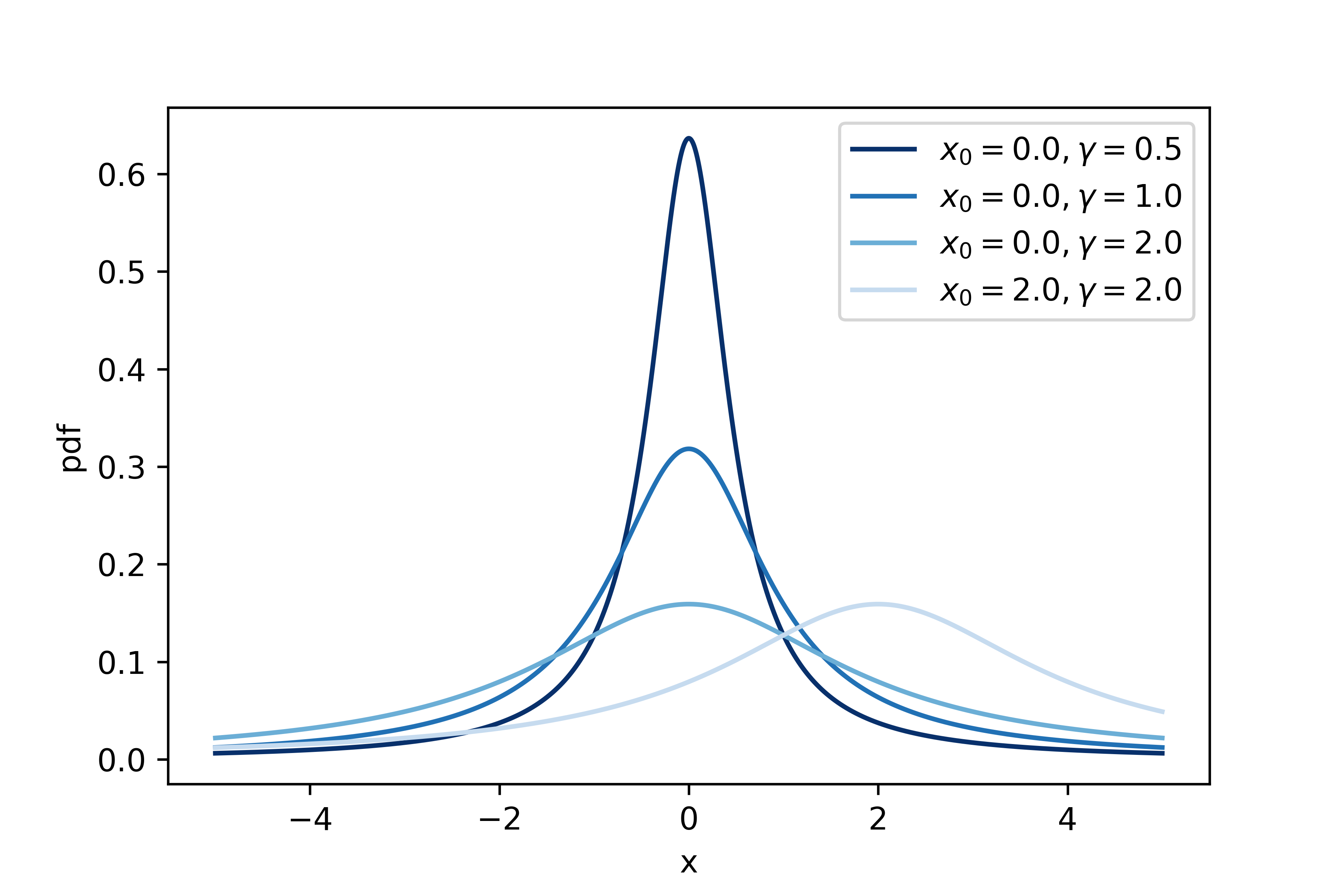
The Cauchy distribution is a family of continuous probability distributions, which is stable and has a probability density function (PDF), which can be expressed analytically. As compared to the Gaussian distribution, the Cauchy distribution has a higher peak and a longer tail. The Cauchy distribution has two parameters: the location parameter and the scale parameter . The Cauchy distribution has a short and wide PDF if the scale parameter is high, while a tall and narrow PDF if the scale parameter is low. The PDF of the Cauchy distribution with and can be defined as follows.
| (6) |
Additionally, the cumulative distribution function of the Cauchy distribution with and can be defined as follows.
| (7) |
Fig. 1 shows the four different PDFs of the Cauchy distribution.
3 Literature Review
Since it was introduced, many researchers have developed new methods for DE, such as
- 1.
- 2.
- 3.
- 4.
Among numerous DE variants, L-SHADE variants [7, 8, 9, 10, 11, 12, 13, 14, 15, 16, 17, 18] frequently perform very well on various optimization problems. JADE [7] proposed by Zhang and Sanderson is considered to be the origin of L-SHADE variants. JADE uses a new mutation strategy DE/current-to-best/1 with an external archive. The new mutation strategy is the generalization of a classical mutation strategy DE/current-to-best/1, and the external archive supplies the progress of an evolutionary process. These modifications improve the exploration of the algorithm. JADE also uses a learning process-based adaptive parameter control to adjust the control parameters and automatically. In the experiments, JADE outperformed several algorithms, including jDE [29], SaDE [38], and PSO [59].
Tanabe and Fukunaga proposed SHADE [8], an enhancement to JADE. The main difference between SHADE and JADE is that SHADE utilizes historical memories, which store the average of successfully evolved individuals’ control parameters and to adjust the control parameters and automatically. In the experiments, SHADE outperformed several algorithms, including CoDE [40], EPSDE [39], and dynNP-DE [30]. Tanabe and Fukunaga later proposed L-SHADE [9], an enhancement to SHADE. The main difference between L-SHADE and SHADE is that L-SHADE utilizes linear population size reduction (LPSR), which gradually reduces the population size as a linear function to establish a balance between exploration and exploitation. In the experiments, L-SHADE outperformed several algorithms, including NBIPOP-CMA-ES [60] and iCMAES-ILS [61].
Brest et al. proposed an improved version of L-SHADE called iL-SHADE [10]. iL-SHADE updates historical memories and by calculating the average of old and new values. iL-SHADE also gradually reduces the value of DE/current-to-best/1 as a linear function. iL-SHADE was ranked third place in the CEC 2016 competition on single objective real-valued optimization. Brest et al. later proposed an improved version of iL-SHADE called jSO [11]. jSO uses a new mutation strategy DE/current-to-best-w/1, which assigns a lower scaling factor at the early stage of an evolutionary process and a higher scaling factor at the late stage of an evolutionary process. jSO was ranked second place in the CEC 2017 competitions on single objective real-valued optimization.
Awad et al. proposed LSHADE-EpSin [12] based on L-SHADE, which utilizes a new ensemble sinusoidal approach for tuning the scaling factor in an adaptive manner. The new ensemble sinusoidal approach is the combination of two sinusoidal waves whose objective is to establish a balance between exploration and exploitation. LSHADE-EpSin also utilizes a random walk at the late stage of an evolutionary process. Awad et al. proposed L-SHADE [13] based on L-SHADE, which utilizes a new crossover operator based on covariance matrix adaptation with Euclidean neighborhood for rotation invariance. Awad et al. later proposed LSHADE-EpSin [14], which is the combination of LSHADE-EpSin and L-SHADE with two major modifications: 1) a new ensemble sinusoidal approach with a learning process-based adaptive parameter control and 2) a new crossover operator based on covariance matrix adaptation with Euclidean neighborhood for rotation invariance. Finally, Awad et al. proposed EsDE-NR [15] based on LSHADE-EpSin, which gradually reduces the population size with a niching-based approach.
Mohamed et al. proposed LSHADE-SPACMA [16], an enhancement to L-SHADE, which is a hybrid algorithm between LSHADE-SPA [16] and a modified version of CMA-ES [62]. LSHADE-SPA uses a new semi-parameter control for tuning the scaling factor in an adaptive manner. The modified version of CMA-ES undergoes the phase of the crossover, which improves the exploration of the algorithm.
Yet et al. propose mL-SHADE [18], an enhancement to L-SHADE, in which three major modifications are made: 1) a terminal value for the control parameter is excluded, 2) a polynomial mutation strategy is included, and 3) a perturbation for historical memories is included. These modifications improve the exploration of the algorithm.
4 Proposed Algorithm
This section describes an improved LSHADE-RSP called iLSHADE-RSP, which employs a modified recombination operator, which calculates a perturbation of a target vector with the Cauchy distribution.
4.1 Mutation Strategy
The proposed algorithm uses a new mutation strategy DE/current-to-best/r [17]. The strategy is designed based on a rank-based selective pressure scheme [63], which proportionally selects two donor vectors and with respect to the fitness value. The higher the ranking of a candidate solution has, the more opportunity it will be selected. The strategy can be defined as follows.
-
1.
DE/current-to-best/r:
where
where denotes one of the top individuals with . Also, denotes a random donor vector from a population based on rank-based probabilities, and denotes a random donor vector from a population based on rank-based probabilities or from an external archive. The probability of the th individual being selected can be calculated as follows.
| (8) |
where
| (9) |
where denotes a rank greediness factor. Additionally, LSHADE-RSP uses a setting for increasing the number of best individuals, which can be calculated as follows.
| (10) |
4.2 Linear Population Size Reduction
The proposed algorithm uses linear population size reduction (LPSR) [9] to establish a balance between exploration and exploitation. The idea behind LPSR is to use a higher population size at the beginning of an optimization process and gradually reduce it as a linear function. At the end of each generation, LPSR calculates the population size for the next generation as follows.
| (11) |
where and denote the initial and final population sizes, respectively. If the next population size is smaller than the current one , the worst candidate solutions with respect to the fitness value are discarded. For the initial and final population sizes, LSHADE-RSP uses and .
4.2.1 Adaptive Parameter Control
The proposed algorithm uses a learning process-based adaptive parameter control [11] to adjust the control parameters and automatically. Each candidate solution has its control parameters and . At each generation, the control parameters and are calculated as follows.
| (12) |
| (13) |
where and denote the Cauchy and Gaussian distributions, respectively. Also, and denote randomly selected values from historical memories and , respectively. The scaling factor is recalculated if or truncated to 1 if . The crossover rate is first truncated to . After that, the crossover rate is modified as follows.
The historical memories and store the successfully evolved candidate solutions’ control parameters. The capacity of the historical memories is . At the beginning of an optimization process, all the entries, except the last one, of the memory are initialized to 0.3. Similarly, all the entries, except the last one, of the memory are initialized to 0.8. The last entry of the memories and always keep 0.9 during the optimization process. After the selection operator, the successfully evolved candidate solutions’ control parameters are stored in and . Then, one of the entries of the memories is updated as follows.
| (14) |
| (15) |
where denotes the weighted Lehmer mean, which takes into consideration the improvement in fitness values between candidate solutions and their corresponding offspring.
4.3 Cauchy Perturbation
LSHADE-RSP [17] uses a rank-based selective pressure scheme, which tends to select higher ranking candidate solutions as donor vectors. Therefore, the scheme can increase the greediness, which can boost the convergence speed. However, the scheme may decrease the solution accuracy because of premature convergence in which all the candidate solutions fall into the local optimum of an optimization problem and cannot escape from there [19, 20, 21, 22]. Although LSHADE-RSP uses a setting for increasing the number of best individuals, it may not be sufficient to compensate for the increased greediness.
To improve the exploration property of EAs, many researchers have developed new methods. Among them, using a long-tailed stable distribution, such as the Cauchy or Lévy distribution, in the phase of the recombination is one of the popular ones. By using a long-tailed stable distribution, EAs can generate candidate solutions over large distances, which can improve the exploration property. In the literature of DE, some researchers have demonstrated the effectiveness of using a long-tailed stable distribution in the phase of the recombination [26, 27, 25]. This motivated us to devise a modified recombination operator for LSHADE-RSP.
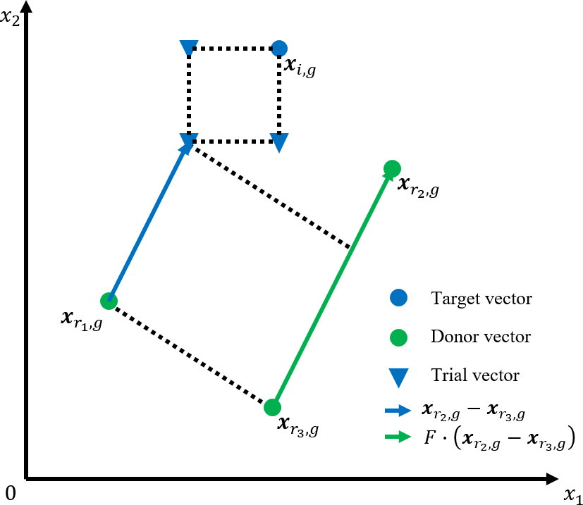
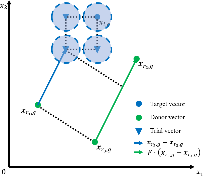
The idea behind the modified recombination operator is simple. When creating a trial vector, the operator first perturbs a target vector with the Cauchy distribution. After that, the operator creates a trial vector by recombining the perturbed target vector and its corresponding mutant vector. Therefore, a much different trial vector can be created by adopting the long-tail property of the Cauchy distribution. The novelty of the proposed approach lies in the perturbation of a target vector instead of a mutant vector. Fig. 2 illustrates the behavior of the modified recombination operator with DE/rand/1/bin.
As we mentioned earlier, the modified recombination operator is an extension of the recombination operator of LSHADE-RSP. The original operator can be defined as follows.
| (16) |
where denotes the th component of one of the top individuals with . Also, denotes the th component of a random donor vector from a population based on rank-based probabilities, and denotes the th component of a random donor vector from a population based on rank-based probabilities or from an external archive. The modified operator can be defined as follows.
| (17) |
where denotes the Cauchy distribution.
The proposed algorithm alternately applies one of the two recombination operators according to the jumping rate . When creating a trial vector, the proposed algorithm applies the original operator if a random number is higher than or equal to the rate. Otherwise, the proposed algorithm applies the modified operator. Algorithm 1 shows the pseudo-code of the proposed algorithm.
5 Experimental Setup
5.1 System Configuration
All the following experiments were performed on Windows 10 Pro 64 bit of a PC with AMD Ryzen Threadripper 2990WX @ 3.0GHz. The proposed and comparison algorithms were developed in the C++ programming language with Visual Studio 2019 64 bit.
5.2 Test Algorithms
We used the following test algorithms for the comparative analysis.
-
1.
iLSAHDE-RSP: the proposed algorithm.
-
2.
LSHADE-RSP [17]: ranked the second place in the CEC 2018 competition on single objective optimization.
-
3.
jSO [11]: ranked the second place in the CEC 2017 competition on single objective optimization.
-
4.
L-SHADE [9]: ranked the first place in the CEC 2014 competition on single objective optimization.
-
5.
SHADE [8]: ranked the fourth place in the CEC 2013 competition on single objective optimization.
-
6.
JADE [7]: the origin of L-SHADE variants.
-
7.
EDEV [46]: a multi-population-based DE variant.
-
8.
MPEDE [45]: a multi-population-based DE variant.
-
9.
CoDE [40]: a composite DE variant.
-
10.
EPSDE [39]: an ensemble DE variant.
-
11.
SaDE [38]: a self-adaptive DE variant.
-
12.
dynNP-DE [30]: a self-adaptive DE variant.
The algorithms are six L-SHADE variants, two multi-population-based DE variants, and four well-known classical DE variants. The proposed algorithm introduces the jumping rate . As shown in Section 6, the proposed algorithm works best with . The proposed algorithm uses in all the following experiments. Except for the jumping rate, the proposed algorithm uses the same values for the control parameters as its predecessor LSHADE-RSP.
5.3 Test Functions
To compare the proposed and comparison algorithms experimentally, we carried out experiments on the CEC 2017 test suite [28] in 10, 30, 50 and 100 dimensions. The CEC 2017 test suite has 30 different and difficult optimization problems, such as three unimodal test functions (-), seven simple multimodal test functions (-), ten expanded multimodal test functions (-), and ten hybrid composition test functions (-). A function is said to be unimodal if it has no local optima, while a function is said to be multimodal if it has multiple local optima.
According to the experimental setups of the test suite, the maximum number of function evaluations was set to . Moreover, the search boundaries of the test suite were set to . Furthermore, all the experimental results were obtained by 51 runs independently. For more detailed information, please refer to the following papers [28].
5.4 Performance Metrics
5.4.1 Function Error Value
The function error value (FEV) is utilized to assess the test algorithm’s accuracy. The FEV is the difference between the final best objective value of a test algorithm and the global optimum of an optimization problem, which can be defined as follows.
| (18) |
where denotes an objective function. Also, and denote the final best objective value and the global optimum, respectively.
5.4.2 Statistical Test
We utilized the Wilcoxon rank-sum test and the Friedman test with Hochberg’s post hoc for the comparative analysis. The former is used to test the statistical significance of two test algorithms, while the latter is used to test the statistical significance of multiple test algorithms [64].
6 Experimental Results and Discussion
| iLSHADE-RSP | LSHADE-RSP | jSO | L-SHADE | SHADE | JADE | EDEV | |
| MEAN (STD DEV) | MEAN (STD DEV) | MEAN (STD DEV) | MEAN (STD DEV) | MEAN (STD DEV) | MEAN (STD DEV) | MEAN (STD DEV) | |
| F1 | 0.00E+00 (0.00E+00) | 0.00E+00 (0.00E+00) = | 0.00E+00 (0.00E+00) = | 0.00E+00 (0.00E+00) = | 0.00E+00 (0.00E+00) = | 0.00E+00 (0.00E+00) = | 0.00E+00 (0.00E+00) = |
| F2 | 0.00E+00 (0.00E+00) | 0.00E+00 (0.00E+00) = | 0.00E+00 (0.00E+00) = | 0.00E+00 (0.00E+00) = | 0.00E+00 (0.00E+00) = | 0.00E+00 (0.00E+00) = | 1.23E-09 (4.12E-09) = |
| F3 | 0.00E+00 (0.00E+00) | 0.00E+00 (0.00E+00) = | 0.00E+00 (0.00E+00) = | 0.00E+00 (0.00E+00) = | 0.00E+00 (0.00E+00) = | 0.00E+00 (0.00E+00) = | 0.00E+00 (0.00E+00) = |
| F4 | 0.00E+00 (0.00E+00) | 0.00E+00 (0.00E+00) = | 0.00E+00 (0.00E+00) = | 0.00E+00 (0.00E+00) = | 0.00E+00 (0.00E+00) = | 0.00E+00 (0.00E+00) = | 0.00E+00 (0.00E+00) = |
| F5 | 1.29E+00 (8.03E-01) | 1.29E+00 (9.39E-01) = | 1.83E+00 (8.74E-01) - | 2.46E+00 (9.21E-01) - | 2.64E+00 (7.38E-01) - | 3.48E+00 (8.39E-01) - | 4.68E+00 (9.38E-01) - |
| F6 | 2.91E-14 (5.02E-14) | 1.56E-14 (3.96E-14) = | 0.00E+00 (0.00E+00) + | 0.00E+00 (0.00E+00) + | 2.24E-15 (1.60E-14) + | 8.94E-14 (4.74E-14) - | 2.89E-12 (8.26E-12) - |
| F7 | 1.20E+01 (6.28E-01) | 1.18E+01 (4.92E-01) = | 1.21E+01 (6.40E-01) = | 1.20E+01 (7.14E-01) = | 1.29E+01 (7.39E-01) - | 1.37E+01 (8.66E-01) - | 1.54E+01 (1.28E+00) - |
| F8 | 1.56E+00 (8.02E-01) | 1.37E+00 (9.32E-01) = | 2.01E+00 (7.82E-01) - | 2.61E+00 (8.56E-01) - | 2.55E+00 (8.80E-01) - | 3.59E+00 (9.42E-01) - | 5.37E+00 (1.19E+00) - |
| F9 | 0.00E+00 (0.00E+00) | 0.00E+00 (0.00E+00) = | 0.00E+00 (0.00E+00) = | 0.00E+00 (0.00E+00) = | 0.00E+00 (0.00E+00) = | 0.00E+00 (0.00E+00) = | 0.00E+00 (0.00E+00) = |
| F10 | 4.01E+01 (7.47E+01) | 2.18E+01 (4.56E+01) = | 4.67E+01 (5.92E+01) = | 2.96E+01 (4.19E+01) = | 5.85E+01 (5.46E+01) - | 7.73E+01 (5.30E+01) - | 2.12E+02 (7.48E+01) - |
| F11 | 0.00E+00 (0.00E+00) | 0.00E+00 (0.00E+00) = | 0.00E+00 (0.00E+00) = | 1.01E-01 (4.11E-01) = | 7.72E-01 (8.91E-01) - | 2.36E+00 (6.89E-01) - | 2.11E+00 (6.85E-01) - |
| F12 | 3.55E-01 (2.09E-01) | 3.71E-01 (1.63E-01) = | 2.89E+00 (1.68E+01) = | 3.11E+01 (5.22E+01) - | 9.18E+01 (7.31E+01) - | 9.22E+01 (7.82E+01) - | 1.06E+02 (8.74E+01) - |
| F13 | 3.19E+00 (2.39E+00) | 3.25E+00 (2.39E+00) = | 2.91E+00 (2.46E+00) = | 3.74E+00 (2.14E+00) = | 3.39E+00 (2.44E+00) = | 4.32E+00 (3.06E+00) = | 5.75E+00 (2.06E+00) - |
| F14 | 1.95E-02 (1.39E-01) | 1.56E-01 (3.65E-01) = | 1.17E-01 (3.24E-01) = | 2.23E-01 (4.39E-01) - | 1.96E-01 (2.14E-01) - | 8.75E-01 (4.51E-01) - | 1.16E+00 (5.09E-01) - |
| F15 | 2.14E-01 (2.25E-01) | 2.00E-01 (2.26E-01) = | 3.46E-01 (1.94E-01) - | 1.57E-01 (2.01E-01) = | 2.50E-01 (1.46E-01) = | 4.72E-01 (1.91E-01) - | 6.73E-01 (3.17E-01) - |
| F16 | 5.12E-01 (2.51E-01) | 5.52E-01 (3.04E-01) = | 5.36E-01 (2.72E-01) = | 2.84E-01 (1.47E-01) + | 5.26E-01 (1.82E-01) = | 1.46E+00 (7.72E-01) - | 2.93E+00 (1.42E+00) - |
| F17 | 6.29E-01 (4.22E-01) | 6.49E-01 (4.42E-01) = | 3.59E-01 (3.22E-01) + | 1.29E-01 (1.43E-01) + | 3.69E-01 (2.07E-01) + | 5.02E-01 (2.31E-01) = | 1.85E+00 (7.46E-01) - |
| F18 | 1.78E-01 (1.96E-01) | 2.06E-01 (2.18E-01) = | 2.35E-01 (2.13E-01) = | 2.56E-01 (2.12E-01) = | 5.85E-01 (2.81E+00) = | 5.02E-01 (6.57E-01) - | 1.97E+00 (4.83E+00) - |
| F19 | 1.24E-02 (9.75E-03) | 1.03E-02 (1.05E-02) = | 1.03E-02 (1.19E-02) = | 8.84E-03 (9.37E-03) = | 6.01E-02 (2.12E-01) - | 4.75E-02 (2.27E-02) - | 1.29E-01 (9.10E-02) - |
| F20 | 4.22E-01 (1.63E-01) | 4.53E-01 (1.57E-01) = | 3.18E-01 (1.59E-01) + | 0.00E+00 (0.00E+00) + | 1.84E-02 (7.41E-02) + | 1.07E-07 (3.84E-07) + | 1.84E-02 (7.41E-02) + |
| F21 | 1.16E+02 (3.77E+01) | 1.16E+02 (3.76E+01) = | 1.36E+02 (4.98E+01) = | 1.41E+02 (5.07E+01) - | 1.27E+02 (4.29E+01) - | 1.51E+02 (4.88E+01) - | 1.13E+02 (3.47E+01) = |
| F22 | 1.00E+02 (0.00E+00) | 1.00E+02 (0.00E+00) = | 9.89E+01 (7.76E+00) = | 1.00E+02 (0.00E+00) = | 9.64E+01 (1.80E+01) = | 9.60E+01 (1.70E+01) = | 7.59E+01 (4.20E+01) + |
| F23 | 3.01E+02 (1.64E+00) | 2.95E+02 (4.22E+01) = | 3.02E+02 (1.74E+00) = | 3.03E+02 (1.56E+00) - | 3.03E+02 (1.59E+00) - | 3.05E+02 (1.47E+00) - | 3.06E+02 (1.31E+00) - |
| F24 | 2.49E+02 (1.16E+02) | 2.53E+02 (1.09E+02) = | 2.67E+02 (1.03E+02) = | 3.18E+02 (5.17E+01) - | 2.79E+02 (9.13E+01) = | 2.90E+02 (8.16E+01) - | 2.24E+02 (1.18E+02) = |
| F25 | 4.07E+02 (1.80E+01) | 4.00E+02 (8.82E+00) = | 4.09E+02 (1.94E+01) = | 4.12E+02 (2.13E+01) = | 4.17E+02 (2.27E+01) - | 4.18E+02 (2.28E+01) - | 4.07E+02 (1.82E+01) = |
| F26 | 3.00E+02 (0.00E+00) | 3.00E+02 (0.00E+00) = | 3.00E+02 (0.00E+00) = | 3.00E+02 (0.00E+00) = | 3.00E+02 (0.00E+00) = | 2.94E+02 (4.20E+01) = | 3.00E+02 (0.00E+00) = |
| F27 | 3.86E+02 (2.67E+00) | 3.90E+02 (4.28E-01) - | 3.90E+02 (3.85E-01) - | 3.90E+02 (4.01E-01) - | 3.90E+02 (1.40E+00) - | 3.89E+02 (5.66E-01) - | 3.89E+02 (9.00E-01) - |
| F28 | 3.08E+02 (3.92E+01) | 3.14E+02 (6.03E+01) = | 3.28E+02 (8.53E+01) = | 3.40E+02 (1.02E+02) = | 3.91E+02 (1.38E+02) - | 3.63E+02 (1.22E+02) = | 3.00E+02 (0.00E+00) = |
| F29 | 2.34E+02 (3.56E+00) | 2.34E+02 (2.97E+00) = | 2.36E+02 (3.19E+00) = | 2.34E+02 (2.54E+00) = | 2.43E+02 (6.32E+00) - | 2.44E+02 (5.07E+00) - | 2.49E+02 (5.39E+00) - |
| F30 | 3.84E+02 (3.29E+01) | 3.95E+02 (0.00E+00) - | 2.49E+04 (1.75E+05) - | 1.64E+04 (1.14E+05) - | 4.20E+02 (2.74E+01) - | 3.26E+04 (1.60E+05) - | 1.16E+03 (1.43E+03) - |
| +/=/- | 0/28/2 | 3/22/5 | 4/17/9 | 3/12/15 | 1/10/19 | 2/10/18 | |
| MPEDE | CoDE | EPSDE | SaDE | dynNP-DE | |||
| MEAN (STD DEV) | MEAN (STD DEV) | MEAN (STD DEV) | MEAN (STD DEV) | MEAN (STD DEV) | |||
| F1 | 1.72E+02 (4.59E+02) - | 3.18E-05 (2.96E-05) - | 0.00E+00 (0.00E+00) = | 9.18E+02 (2.22E+03) - | 0.00E+00 (0.00E+00) = | ||
| F2 | 1.88E-01 (1.34E+00) - | 2.33E-06 (1.68E-06) - | 4.77E-08 (1.17E-07) - | 1.12E-04 (5.93E-04) - | 1.39E-14 (9.55E-14) = | ||
| F3 | 3.87E-06 (2.51E-05) - | 4.27E-02 (7.38E-02) - | 0.00E+00 (0.00E+00) = | 8.14E-11 (4.00E-10) - | 0.00E+00 (0.00E+00) = | ||
| F4 | 4.19E-02 (2.81E-01) - | 3.43E-04 (1.97E-04) - | 0.00E+00 (0.00E+00) = | 7.57E-02 (5.28E-01) - | 1.72E-01 (1.90E-01) - | ||
| F5 | 8.21E+00 (1.53E+00) - | 8.32E+00 (1.72E+00) - | 4.25E+00 (1.17E+00) - | 4.12E+00 (1.01E+00) - | 6.41E+00 (3.56E+00) - | ||
| F6 | 5.56E-05 (2.25E-05) - | 8.05E-14 (5.25E-14) - | 0.00E+00 (0.00E+00) + | 1.34E-14 (3.71E-14) = | 0.00E+00 (0.00E+00) + | ||
| F7 | 1.99E+01 (1.63E+00) - | 2.10E+01 (3.05E+00) - | 1.54E+01 (1.45E+00) - | 1.62E+01 (1.30E+00) - | 2.18E+01 (5.34E+00) - | ||
| F8 | 8.60E+00 (2.26E+00) - | 9.12E+00 (1.89E+00) - | 4.66E+00 (1.30E+00) - | 4.63E+00 (1.12E+00) - | 7.19E+00 (3.61E+00) - | ||
| F9 | 7.52E-11 (8.70E-11) - | 0.00E+00 (0.00E+00) = | 0.00E+00 (0.00E+00) = | 9.86E-11 (6.50E-10) - | 0.00E+00 (0.00E+00) = | ||
| F10 | 4.06E+02 (9.26E+01) - | 4.02E+02 (1.18E+02) - | 1.79E+02 (8.55E+01) - | 1.70E+02 (8.52E+01) - | 2.90E+02 (2.61E+02) - | ||
| F11 | 3.41E+00 (6.36E-01) - | 5.61E-01 (6.85E-01) - | 1.80E+00 (1.06E+00) - | 2.19E+00 (1.35E+00) - | 3.25E-01 (4.67E-01) - | ||
| F12 | 3.64E+04 (1.20E+05) - | 2.03E+03 (1.09E+03) - | 2.22E+02 (2.07E+02) - | 8.25E+03 (2.49E+04) - | 1.15E+00 (3.00E+00) = | ||
| F13 | 1.03E+02 (9.72E+01) - | 8.48E+00 (3.12E+00) - | 5.32E+00 (2.76E+00) - | 4.16E+00 (3.43E+00) = | 2.08E+00 (2.33E+00) = | ||
| F14 | 1.08E+01 (2.33E+00) - | 6.52E-05 (2.81E-04) - | 3.03E-01 (3.94E-01) - | 4.96E-01 (5.37E-01) - | 4.68E-01 (5.75E-01) - | ||
| F15 | 3.75E+00 (6.97E-01) - | 5.22E-01 (3.15E-01) - | 2.92E-01 (4.64E-01) = | 3.52E-01 (3.97E-01) = | 1.32E-01 (1.83E-01) = | ||
| F16 | 5.91E+00 (2.34E+00) - | 6.40E-01 (3.42E-01) = | 8.34E-01 (4.22E-01) - | 1.91E+00 (1.08E+00) - | 3.38E-01 (2.33E-01) + | ||
| F17 | 1.28E+01 (2.76E+00) - | 2.68E-01 (2.02E-01) + | 1.68E-01 (1.77E-01) + | 6.29E-01 (3.93E-01) = | 5.71E-01 (6.45E-01) + | ||
| F18 | 9.83E+01 (1.30E+02) - | 4.56E-01 (2.36E-01) - | 7.12E+00 (9.67E+00) - | 3.81E-01 (5.38E-01) - | 5.97E-02 (1.30E-01) + | ||
| F19 | 2.19E+00 (4.34E-01) - | 5.18E-02 (2.58E-02) - | 3.48E-03 (5.60E-03) = | 2.05E+01 (6.17E+00) - | 7.61E-03 (9.57E-03) + | ||
| F20 | 2.21E+00 (9.06E-01) - | 3.06E-02 (9.37E-02) + | 1.10E-01 (1.63E-01) + | 1.83E-02 (6.04E-02) + | 1.59E-01 (1.91E-01) + | ||
| F21 | 1.24E+02 (3.00E+01) - | 1.46E+02 (5.54E+01) - | 1.61E+02 (5.34E+01) - | 1.33E+02 (4.63E+01) - | 1.21E+02 (4.29E+01) = | ||
| F22 | 9.83E+01 (1.19E+01) = | 8.16E+01 (4.07E+01) - | 9.07E+01 (2.86E+01) = | 9.70E+01 (1.52E+01) = | 7.54E+01 (4.29E+01) = | ||
| F23 | 3.09E+02 (1.72E+00) - | 3.09E+02 (2.25E+00) - | 3.06E+02 (1.48E+00) - | 3.06E+02 (1.18E+00) - | 3.06E+02 (2.06E+00) - | ||
| F24 | 2.65E+02 (8.54E+01) - | 2.83E+02 (1.03E+02) - | 3.10E+02 (6.99E+01) - | 2.23E+02 (1.10E+02) = | 2.23E+02 (1.17E+02) = | ||
| F25 | 4.03E+02 (1.46E+01) = | 4.00E+02 (9.02E+00) = | 4.20E+02 (2.29E+01) - | 4.08E+02 (1.87E+01) = | 3.98E+02 (0.00E+00) = | ||
| F26 | 3.00E+02 (0.00E+00) = | 3.00E+02 (0.00E+00) = | 3.00E+02 (0.00E+00) = | 3.00E+02 (0.00E+00) = | 3.00E+02 (0.00E+00) = | ||
| F27 | 3.89E+02 (5.02E-01) - | 3.88E+02 (1.03E+00) - | 3.90E+02 (1.75E+00) - | 3.90E+02 (7.79E-01) - | 3.89E+02 (9.23E-01) - | ||
| F28 | 3.00E+02 (0.00E+00) = | 3.00E+02 (0.00E+00) = | 3.31E+02 (8.95E+01) = | 3.01E+02 (5.85E+01) = | 3.00E+02 (0.00E+00) = | ||
| F29 | 2.55E+02 (6.25E+00) - | 2.50E+02 (6.93E+00) - | 2.46E+02 (3.72E+00) - | 2.42E+02 (9.24E+00) - | 2.31E+02 (2.76E+00) + | ||
| F30 | 4.34E+03 (4.90E+03) - | 1.03E+03 (5.21E+02) - | 3.27E+04 (1.60E+05) - | 6.82E+02 (6.40E+02) - | 4.01E+02 (8.43E+00) - | ||
| +/=/- | 0/4/26 | 2/5/23 | 3/9/18 | 1/9/20 | 7/13/10 |
The symbols “+/=/-” indicate that the corresponding algorithm performed significantly better (), not significantly better or worse (), or significantly worse () compared to iLSHADE-RSP using the Wilcoxon rank-sum test with significance level.
| Algorithm | Average ranking | z-value | p-value | Adj. p-value (Hochberg) | Sig. | Test statistics | |||
|---|---|---|---|---|---|---|---|---|---|
| 1 | iLSHADE-RSP | 4.15 | |||||||
| 2 | LSHADE-RSP | 4.42 | -2.86.E-01 | 7.75.E-01 | 7.75.E-01 | No | N | 30 | |
| 3 | jSO | 5.30 | -1.24.E+00 | 2.17.E-01 | 8.67.E-01 | No | Chi-Square | 76.90 | |
| 4 | L-SHADE | 5.23 | -1.16.E+00 | 2.45.E-01 | 7.34.E-01 | No | df | 11 | |
| 5 | SHADE | 6.12 | -2.11.E+00 | 3.46.E-02 | 1.73.E-01 | No | p-value | 5.85.E-12 | |
| 6 | JADE | 7.05 | -3.12.E+00 | 1.84.E-03 | 1.10.E-02 | Yes | Sig. | Yes | |
| 7 | EDEV | 7.35 | -3.44.E+00 | 5.87.E-04 | 4.11.E-03 | Yes | |||
| 8 | MPEDE | 9.97 | -6.25.E+00 | 4.15.E-10 | 4.57.E-09 | Yes | |||
| 9 | CoDE | 7.87 | -3.99.E+00 | 6.54.E-05 | 5.89.E-04 | Yes | |||
| 10 | EPSDE | 7.62 | -3.72.E+00 | 1.96.E-04 | 1.57.E-03 | Yes | |||
| 11 | SaDE | 7.90 | -4.03.E+00 | 5.62.E-05 | 5.62.E-04 | Yes | |||
| 12 | dynNP-DE | 5.03 | -9.49.E-01 | 3.43.E-01 | 6.85.E-01 | No |
| iLSHADE-RSP | LSHADE-RSP | jSO | L-SHADE | SHADE | JADE | EDEV | |
| MEAN (STD DEV) | MEAN (STD DEV) | MEAN (STD DEV) | MEAN (STD DEV) | MEAN (STD DEV) | MEAN (STD DEV) | MEAN (STD DEV) | |
| F1 | 1.67E-15 (4.62E-15) | 8.35E-16 (3.37E-15) = | 2.78E-16 (1.99E-15) = | 2.78E-16 (1.99E-15) = | 1.36E-14 (3.98E-15) - | 1.42E-14 (1.27E-29) - | 2.78E-16 (1.99E-15) = |
| F2 | 0.00E+00 (0.00E+00) | 0.00E+00 (0.00E+00) = | 0.00E+00 (0.00E+00) = | 2.78E-15 (8.53E-15) = | 5.59E-13 (1.01E-12) - | 3.61E-13 (5.66E-13) - | 1.05E+13 (6.16E+13) - |
| F3 | 2.56E-14 (2.85E-14) | 1.89E-14 (2.70E-14) = | 7.80E-15 (1.97E-14) + | 5.57E-15 (1.71E-14) + | 7.25E-14 (2.58E-14) - | 9.43E+03 (1.54E+04) - | 4.98E+03 (1.28E+04) = |
| F4 | 2.27E+01 (7.02E-01) | 5.86E+01 (5.74E-14) - | 5.86E+01 (5.74E-14) - | 5.87E+01 (7.70E-01) - | 3.62E+01 (2.98E+01) = | 4.88E+01 (2.39E+01) - | 5.16E+01 (2.09E+01) - |
| F5 | 7.89E+00 (2.38E+00) | 7.11E+00 (2.09E+00) = | 8.85E+00 (1.91E+00) = | 6.77E+00 (1.60E+00) = | 1.91E+01 (3.29E+00) - | 2.63E+01 (4.00E+00) - | 3.41E+01 (4.74E+00) - |
| F6 | 5.77E-08 (1.34E-07) | 6.04E-09 (2.71E-08) = | 7.38E-09 (2.77E-08) = | 2.69E-09 (1.92E-08) = | 2.41E-08 (1.53E-07) = | 2.38E-13 (4.70E-14) - | 1.29E-11 (6.60E-11) - |
| F7 | 4.08E+01 (3.42E+00) | 3.95E+01 (2.50E+00) + | 3.96E+01 (2.10E+00) + | 3.77E+01 (1.42E+00) + | 4.90E+01 (3.56E+00) - | 5.46E+01 (4.02E+00) - | 6.13E+01 (4.25E+00) - |
| F8 | 7.93E+00 (2.39E+00) | 7.38E+00 (2.28E+00) = | 8.85E+00 (2.36E+00) = | 7.24E+00 (1.59E+00) = | 2.08E+01 (2.86E+00) - | 2.64E+01 (3.83E+00) - | 3.17E+01 (5.62E+00) - |
| F9 | 0.00E+00 (0.00E+00) | 0.00E+00 (0.00E+00) = | 0.00E+00 (0.00E+00) = | 0.00E+00 (0.00E+00) = | 6.04E-14 (5.75E-14) - | 3.51E-03 (1.75E-02) = | 1.75E-03 (1.25E-02) = |
| F10 | 1.90E+03 (3.46E+02) | 1.92E+03 (3.31E+02) = | 1.64E+03 (3.36E+02) + | 1.49E+03 (1.51E+02) + | 1.78E+03 (2.79E+02) + | 1.92E+03 (2.15E+02) = | 2.40E+03 (3.23E+02) - |
| F11 | 3.41E+00 (5.57E+00) | 2.62E+00 (2.23E+00) = | 4.13E+00 (8.72E+00) = | 2.88E+01 (2.81E+01) - | 2.50E+01 (2.72E+01) - | 3.68E+01 (2.65E+01) - | 3.90E+01 (2.90E+01) - |
| F12 | 1.20E+02 (7.85E+01) | 9.51E+01 (7.16E+01) = | 2.17E+02 (1.14E+02) - | 1.06E+03 (3.76E+02) - | 1.42E+03 (7.73E+02) - | 1.15E+03 (3.87E+02) - | 1.45E+03 (1.21E+03) - |
| F13 | 1.80E+01 (4.92E+00) | 1.73E+01 (5.41E+00) = | 1.55E+01 (4.93E+00) + | 1.72E+01 (4.75E+00) = | 4.32E+01 (2.37E+01) - | 4.79E+01 (5.92E+01) - | 6.05E+01 (7.21E+01) - |
| F14 | 2.17E+01 (1.06E+00) | 2.15E+01 (1.23E+00) = | 2.24E+01 (1.21E+00) - | 2.16E+01 (1.24E+00) = | 3.10E+01 (6.52E+00) - | 7.30E+03 (1.27E+04) - | 3.46E+01 (1.44E+01) - |
| F15 | 1.08E+00 (7.50E-01) | 1.13E+00 (7.73E-01) = | 9.83E-01 (6.29E-01) = | 3.10E+00 (1.46E+00) - | 2.15E+01 (2.29E+01) - | 7.71E+02 (1.82E+03) - | 2.46E+01 (2.06E+01) - |
| F16 | 1.66E+01 (6.67E+00) | 2.87E+01 (4.35E+01) - | 7.32E+01 (7.71E+01) - | 6.25E+01 (7.43E+01) - | 3.09E+02 (1.34E+02) - | 3.83E+02 (1.45E+02) - | 4.73E+02 (1.10E+02) - |
| F17 | 3.89E+01 (7.18E+00) | 3.78E+01 (7.04E+00) = | 3.49E+01 (9.46E+00) + | 3.31E+01 (6.94E+00) + | 5.19E+01 (1.80E+01) - | 7.70E+01 (3.12E+01) - | 1.01E+02 (2.56E+01) - |
| F18 | 2.08E+01 (2.88E-01) | 2.08E+01 (2.89E-01) = | 2.08E+01 (4.08E-01) + | 2.19E+01 (1.07E+00) - | 9.82E+01 (7.62E+01) - | 1.58E+04 (4.77E+04) - | 2.12E+04 (6.72E+04) - |
| F19 | 3.31E+00 (6.06E-01) | 3.49E+00 (1.08E+00) = | 4.32E+00 (1.40E+00) - | 5.38E+00 (1.40E+00) - | 1.26E+01 (1.07E+01) - | 1.27E+03 (3.62E+03) - | 1.67E+01 (9.42E+00) - |
| F20 | 3.24E+01 (7.02E+00) | 3.38E+01 (9.50E+00) = | 3.04E+01 (8.54E+00) = | 4.10E+01 (8.81E+00) - | 7.80E+01 (5.02E+01) - | 1.21E+02 (6.10E+01) - | 1.31E+02 (5.58E+01) - |
| F21 | 2.08E+02 (2.36E+00) | 2.07E+02 (2.19E+00) = | 2.09E+02 (2.24E+00) - | 2.07E+02 (1.49E+00) + | 2.21E+02 (3.74E+00) - | 2.27E+02 (5.36E+00) - | 2.33E+02 (4.79E+00) - |
| F22 | 1.00E+02 (0.00E+00) | 1.00E+02 (0.00E+00) = | 1.00E+02 (0.00E+00) = | 1.00E+02 (0.00E+00) = | 1.00E+02 (0.00E+00) = | 1.45E+02 (3.18E+02) = | 1.00E+02 (0.00E+00) = |
| F23 | 3.50E+02 (3.29E+00) | 3.51E+02 (3.47E+00) = | 3.52E+02 (3.20E+00) - | 3.49E+02 (2.70E+00) = | 3.65E+02 (5.67E+00) - | 3.74E+02 (6.00E+00) - | 3.78E+02 (5.24E+00) - |
| F24 | 4.26E+02 (2.45E+00) | 4.27E+02 (2.10E+00) = | 4.26E+02 (2.43E+00) = | 4.26E+02 (1.67E+00) = | 4.37E+02 (4.98E+00) - | 4.40E+02 (4.50E+00) - | 4.44E+02 (4.80E+00) - |
| F25 | 3.79E+02 (0.00E+00) | 3.87E+02 (0.00E+00) - | 3.87E+02 (0.00E+00) - | 3.87E+02 (0.00E+00) - | 3.87E+02 (7.84E-01) - | 3.87E+02 (0.00E+00) - | 3.87E+02 (0.00E+00) - |
| F26 | 9.33E+02 (3.92E+01) | 9.38E+02 (3.77E+01) = | 9.35E+02 (3.60E+01) = | 9.28E+02 (3.69E+01) = | 1.12E+03 (1.53E+02) - | 1.18E+03 (1.43E+02) - | 1.27E+03 (6.27E+01) - |
| F27 | 4.79E+02 (6.51E+00) | 4.98E+02 (7.29E+00) - | 4.96E+02 (5.97E+00) - | 5.04E+02 (5.50E+00) - | 5.05E+02 (8.12E+00) - | 5.03E+02 (7.56E+00) - | 5.03E+02 (5.76E+00) - |
| F28 | 3.02E+02 (1.60E+01) | 3.04E+02 (2.23E+01) = | 3.04E+02 (2.23E+01) = | 3.30E+02 (4.86E+01) - | 3.42E+02 (5.80E+01) - | 3.42E+02 (5.91E+01) - | 3.39E+02 (5.59E+01) - |
| F29 | 4.14E+02 (2.72E+01) | 4.46E+02 (1.39E+01) - | 4.38E+02 (1.87E+01) - | 4.34E+02 (6.46E+00) - | 4.77E+02 (3.53E+01) - | 4.82E+02 (3.84E+01) - | 5.04E+02 (3.34E+01) - |
| F30 | 1.04E+03 (3.21E+02) | 1.97E+03 (1.10E+01) - | 1.97E+03 (1.05E+01) - | 1.98E+03 (4.71E+01) - | 2.14E+03 (1.66E+02) - | 2.35E+03 (1.36E+03) - | 2.55E+03 (2.81E+03) - |
| +/=/- | 1/23/6 | 6/13/11 | 5/12/13 | 1/3/26 | 0/3/27 | 0/4/26 | |
| MPEDE | CoDE | EPSDE | SaDE | dynNP-DE | |||
| MEAN (STD DEV) | MEAN (STD DEV) | MEAN (STD DEV) | MEAN (STD DEV) | MEAN (STD DEV) | |||
| F1 | 8.16E-02 (5.26E-01) = | 5.03E+00 (1.77E+00) - | 4.18E-15 (6.53E-15) = | 6.44E+02 (1.17E+03) - | 5.44E-04 (2.18E-03) - | ||
| F2 | 1.34E+13 (7.88E+13) - | 1.30E+22 (3.78E+22) - | 1.34E+12 (7.09E+12) - | 2.99E+16 (2.10E+17) - | 1.32E+11 (6.29E+11) - | ||
| F3 | 7.85E+03 (1.39E+04) = | 3.15E+04 (5.59E+03) - | 5.00E+03 (9.68E+03) - | 7.12E+03 (1.81E+04) - | 1.03E+01 (3.02E+01) - | ||
| F4 | 5.67E+01 (1.17E+01) - | 8.25E+01 (5.37E+00) - | 2.91E+01 (2.99E+01) = | 4.42E+01 (4.13E+01) = | 7.61E+01 (1.02E+01) - | ||
| F5 | 5.08E+01 (5.83E+00) - | 1.22E+02 (9.30E+00) - | 6.00E+01 (1.05E+01) - | 3.58E+01 (5.80E+00) - | 5.02E+01 (3.81E+01) - | ||
| F6 | 2.10E-13 (1.85E-13) = | 1.01E-04 (3.17E-05) - | 1.14E-13 (7.65E-29) = | 1.78E-13 (5.65E-14) = | 1.63E-06 (4.26E-06) - | ||
| F7 | 8.18E+01 (5.87E+00) - | 1.77E+02 (1.24E+01) - | 9.68E+01 (9.09E+00) - | 7.37E+01 (7.63E+00) - | 1.38E+02 (5.36E+01) - | ||
| F8 | 5.03E+01 (5.36E+00) - | 1.27E+02 (1.06E+01) - | 6.54E+01 (9.78E+00) - | 3.54E+01 (5.54E+00) - | 5.97E+01 (4.63E+01) - | ||
| F9 | 0.00E+00 (0.00E+00) = | 2.05E+02 (6.54E+01) - | 1.60E-01 (3.81E-01) - | 1.18E+00 (1.57E+00) - | 0.00E+00 (0.00E+00) = | ||
| F10 | 3.40E+03 (2.92E+02) - | 4.64E+03 (2.54E+02) - | 3.65E+03 (2.95E+02) - | 2.43E+03 (2.85E+02) - | 5.65E+03 (7.00E+02) - | ||
| F11 | 3.98E+01 (1.89E+01) - | 1.09E+02 (1.83E+01) - | 4.73E+01 (3.52E+01) - | 2.18E+01 (1.73E+01) - | 1.11E+01 (4.25E+00) - | ||
| F12 | 1.12E+03 (3.92E+02) - | 3.53E+06 (1.08E+06) - | 6.31E+03 (8.86E+03) - | 4.90E+04 (9.99E+04) - | 9.10E+03 (7.03E+03) - | ||
| F13 | 2.64E+04 (3.92E+04) - | 8.67E+02 (4.65E+02) - | 1.08E+03 (3.96E+03) - | 3.35E+03 (8.96E+03) - | 2.67E+01 (7.65E+00) - | ||
| F14 | 9.48E+03 (7.38E+03) - | 7.19E+01 (7.68E+00) - | 7.49E+01 (4.28E+01) - | 1.82E+03 (5.27E+03) = | 1.97E+01 (1.20E+01) = | ||
| F15 | 2.22E+04 (1.35E+04) - | 9.21E+01 (2.18E+01) - | 1.14E+02 (1.17E+02) - | 4.53E+03 (8.10E+03) - | 9.69E+00 (2.36E+00) - | ||
| F16 | 5.99E+02 (1.28E+02) - | 5.87E+02 (1.34E+02) - | 4.02E+02 (1.21E+02) - | 3.67E+02 (1.36E+02) - | 2.87E+02 (2.32E+02) - | ||
| F17 | 1.41E+02 (3.06E+01) - | 1.03E+02 (3.52E+01) - | 8.43E+01 (2.42E+01) - | 7.63E+01 (1.25E+01) - | 3.29E+01 (1.24E+01) + | ||
| F18 | 1.13E+05 (1.62E+05) - | 1.13E+04 (9.46E+03) - | 5.36E+02 (6.37E+02) - | 5.20E+04 (7.55E+04) - | 2.18E+01 (8.26E+00) - | ||
| F19 | 1.45E+04 (1.15E+04) - | 4.09E+01 (5.71E+00) - | 8.90E+01 (6.57E+01) - | 9.46E+02 (3.28E+03) - | 5.19E+00 (1.62E+00) - | ||
| F20 | 1.91E+02 (5.22E+01) - | 9.07E+01 (6.49E+01) - | 1.24E+02 (6.42E+01) - | 1.42E+02 (5.83E+01) - | 1.57E+01 (1.90E+01) + | ||
| F21 | 2.50E+02 (5.72E+00) - | 3.25E+02 (9.45E+00) - | 2.63E+02 (9.28E+00) - | 2.37E+02 (4.91E+00) - | 2.41E+02 (2.54E+01) - | ||
| F22 | 1.00E+02 (0.00E+00) = | 1.99E+02 (7.06E+02) = | 1.00E+02 (3.92E-01) = | 1.00E+02 (0.00E+00) = | 1.00E+02 (0.00E+00) = | ||
| F23 | 3.96E+02 (6.41E+00) - | 4.63E+02 (7.91E+00) - | 4.07E+02 (9.73E+00) - | 3.80E+02 (5.83E+00) - | 3.79E+02 (9.86E+00) - | ||
| F24 | 4.60E+02 (7.29E+00) - | 5.55E+02 (1.16E+01) - | 4.76E+02 (9.02E+00) - | 4.52E+02 (7.69E+00) - | 4.54E+02 (1.28E+01) - | ||
| F25 | 3.87E+02 (0.00E+00) - | 3.87E+02 (0.00E+00) - | 3.87E+02 (9.92E-01) - | 3.87E+02 (0.00E+00) - | 3.87E+02 (0.00E+00) - | ||
| F26 | 1.37E+03 (6.61E+01) - | 2.10E+03 (4.67E+02) - | 1.39E+03 (2.40E+02) - | 1.23E+03 (2.04E+02) - | 1.19E+03 (1.33E+02) - | ||
| F27 | 5.02E+02 (4.47E+00) - | 5.11E+02 (3.89E+00) - | 5.01E+02 (9.62E+00) - | 5.06E+02 (5.76E+00) - | 4.85E+02 (8.30E+00) - | ||
| F28 | 3.14E+02 (3.80E+01) = | 4.39E+02 (1.94E+01) - | 3.31E+02 (5.15E+01) - | 3.44E+02 (5.30E+01) - | 3.19E+02 (3.96E+01) - | ||
| F29 | 5.39E+02 (2.51E+01) - | 6.65E+02 (8.67E+01) - | 5.05E+02 (3.84E+01) - | 4.94E+02 (4.48E+01) - | 4.23E+02 (2.68E+01) - | ||
| F30 | 7.97E+03 (8.80E+03) - | 8.92E+03 (2.63E+03) - | 2.40E+03 (8.19E+02) - | 8.23E+03 (6.40E+03) - | 2.11E+03 (8.36E+01) - | ||
| +/=/- | 0/6/24 | 0/1/29 | 0/4/26 | 0/4/26 | 2/3/25 |
The symbols “+/=/-” indicate that the corresponding algorithm performed significantly better (), not significantly better or worse (), or significantly worse () compared to iLSHADE-RSP using the Wilcoxon rank-sum test with significance level.
| Algorithm | Average ranking | z-value | p-value | Adj. p-value (Hochberg) | Sig. | Test statistics | |||
|---|---|---|---|---|---|---|---|---|---|
| 1 | iLSHADE-RSP | 2.85 | |||||||
| 2 | LSHADE-RSP | 3.47 | -6.62.E-01 | 5.08.E-01 | 1.02.E+00 | No | N | 30 | |
| 3 | jSO | 3.40 | -5.91.E-01 | 5.55.E-01 | 5.55.E-01 | No | Chi-Square | 183.61 | |
| 4 | L-SHADE | 3.62 | -8.24.E-01 | 4.10.E-01 | 1.23.E+00 | No | df | 11 | |
| 5 | SHADE | 5.80 | -3.17.E+00 | 1.53.E-03 | 6.12.E-03 | Yes | p-value | 1.84.E-33 | |
| 6 | JADE | 7.50 | -4.99.E+00 | 5.89.E-07 | 3.53.E-06 | Yes | Sig. | Yes | |
| 7 | EDEV | 7.53 | -5.03.E+00 | 4.89.E-07 | 3.42.E-06 | Yes | |||
| 8 | MPEDE | 9.15 | -6.77.E+00 | 1.31.E-11 | 1.31.E-10 | Yes | |||
| 9 | CoDE | 10.90 | -8.65.E+00 | 5.28.E-18 | 5.81.E-17 | Yes | |||
| 10 | EPSDE | 8.80 | -6.39.E+00 | 1.64.E-10 | 1.48.E-09 | Yes | |||
| 11 | SaDE | 8.70 | -6.28.E+00 | 3.30.E-10 | 2.64.E-09 | Yes | |||
| 12 | dynNP-DE | 6.28 | -3.69.E+00 | 2.26.E-04 | 1.13.E-03 | Yes |
| iLSHADE-RSP | LSHADE-RSP | jSO | L-SHADE | SHADE | JADE | EDEV | |
| MEAN (STD DEV) | MEAN (STD DEV) | MEAN (STD DEV) | MEAN (STD DEV) | MEAN (STD DEV) | MEAN (STD DEV) | MEAN (STD DEV) | |
| F1 | 2.03E-14 (1.21E-14) | 1.50E-14 (5.25E-15) = | 1.61E-14 (6.97E-15) = | 1.48E-14 (2.78E-15) = | 6.18E-14 (1.02E-13) - | 6.34E-14 (1.46E-13) - | 4.40E-12 (2.60E-11) = |
| F2 | 9.75E-14 (3.30E-13) | 6.07E-14 (9.54E-14) = | 5.02E-14 (7.95E-14) = | 2.62E-14 (3.63E-14) + | 2.84E-09 (1.20E-08) - | 1.20E-09 (3.80E-09) - | 4.08E+27 (2.91E+28) - |
| F3 | 2.13E-13 (7.51E-14) | 1.30E-13 (3.61E-14) + | 1.21E-13 (4.36E-14) + | 1.32E-13 (3.70E-14) + | 2.82E-13 (1.04E-13) - | 3.18E+04 (4.44E+04) - | 1.74E+04 (4.16E+04) + |
| F4 | 4.76E+01 (4.52E+01) | 3.70E+01 (3.38E+01) - | 4.77E+01 (4.44E+01) - | 7.86E+01 (5.11E+01) - | 3.26E+01 (4.20E+01) = | 4.26E+01 (4.90E+01) = | 5.41E+01 (4.83E+01) = |
| F5 | 1.68E+01 (5.19E+00) | 1.45E+01 (3.54E+00) + | 1.81E+01 (3.92E+00) = | 1.29E+01 (2.45E+00) + | 4.48E+01 (6.17E+00) - | 5.44E+01 (7.50E+00) - | 6.25E+01 (7.84E+00) - |
| F6 | 7.10E-07 (1.04E-06) | 2.16E-07 (3.91E-07) + | 5.93E-07 (1.02E-06) = | 1.22E-04 (5.10E-04) + | 1.01E-05 (2.57E-05) - | 3.43E-13 (5.81E-14) + | 4.75E-13 (5.30E-13) + |
| F7 | 7.21E+01 (8.24E+00) | 7.04E+01 (5.54E+00) = | 6.95E+01 (4.66E+00) = | 6.41E+01 (2.04E+00) + | 9.40E+01 (6.54E+00) - | 1.02E+02 (7.24E+00) - | 1.14E+02 (8.62E+00) - |
| F8 | 1.71E+01 (5.65E+00) | 1.60E+01 (4.54E+00) = | 1.90E+01 (4.64E+00) - | 1.28E+01 (2.10E+00) + | 4.56E+01 (6.37E+00) - | 5.36E+01 (7.35E+00) - | 6.29E+01 (9.25E+00) - |
| F9 | 3.13E-14 (5.14E-14) | 4.47E-15 (2.23E-14) + | 1.34E-14 (3.71E-14) = | 1.79E-14 (4.19E-14) = | 4.99E-01 (5.22E-01) - | 1.14E+00 (1.20E+00) - | 1.03E+00 (1.08E+00) - |
| F10 | 4.16E+03 (6.32E+02) | 4.01E+03 (5.78E+02) = | 3.61E+03 (4.98E+02) + | 3.21E+03 (3.05E+02) + | 3.49E+03 (3.10E+02) + | 3.77E+03 (2.90E+02) + | 4.50E+03 (3.01E+02) - |
| F11 | 1.83E+01 (4.20E+00) | 2.32E+01 (3.51E+00) - | 2.78E+01 (2.97E+00) - | 4.90E+01 (7.59E+00) - | 1.01E+02 (2.69E+01) - | 1.34E+02 (3.48E+01) - | 9.08E+01 (2.58E+01) - |
| F12 | 1.50E+03 (3.25E+02) | 1.59E+03 (4.62E+02) = | 1.77E+03 (3.98E+02) - | 2.28E+03 (4.84E+02) - | 4.55E+03 (2.60E+03) - | 4.39E+03 (2.44E+03) - | 6.15E+03 (3.12E+03) - |
| F13 | 2.75E+01 (1.84E+01) | 3.07E+01 (2.01E+01) = | 3.20E+01 (2.24E+01) = | 5.78E+01 (3.16E+01) - | 3.65E+02 (2.69E+02) - | 2.87E+02 (1.77E+02) - | 5.45E+02 (1.06E+03) - |
| F14 | 2.37E+01 (2.08E+00) | 2.37E+01 (1.89E+00) = | 2.50E+01 (2.28E+00) - | 2.95E+01 (3.15E+00) - | 2.18E+02 (6.74E+01) - | 7.89E+03 (4.05E+04) - | 1.84E+02 (9.20E+01) - |
| F15 | 1.87E+01 (2.10E+00) | 2.07E+01 (2.02E+00) - | 2.32E+01 (2.51E+00) - | 4.10E+01 (9.71E+00) - | 3.27E+02 (1.12E+02) - | 3.05E+02 (1.42E+02) - | 1.86E+02 (8.93E+01) - |
| F16 | 3.15E+02 (1.44E+02) | 3.30E+02 (1.69E+02) = | 4.71E+02 (1.42E+02) - | 3.97E+02 (1.32E+02) - | 7.83E+02 (1.87E+02) - | 8.80E+02 (1.76E+02) - | 9.97E+02 (1.75E+02) - |
| F17 | 2.26E+02 (9.30E+01) | 2.73E+02 (1.14E+02) = | 3.16E+02 (1.11E+02) - | 2.33E+02 (6.86E+01) = | 5.06E+02 (1.20E+02) - | 6.44E+02 (1.34E+02) - | 6.94E+02 (1.04E+02) - |
| F18 | 2.29E+01 (1.48E+00) | 2.31E+01 (1.39E+00) = | 2.41E+01 (1.74E+00) - | 3.78E+01 (1.08E+01) - | 1.88E+02 (9.11E+01) - | 1.77E+02 (1.07E+02) - | 8.04E+04 (2.38E+05) - |
| F19 | 1.06E+01 (2.46E+00) | 1.03E+01 (2.15E+00) = | 1.37E+01 (2.69E+00) - | 2.38E+01 (6.74E+00) - | 1.37E+02 (4.17E+01) - | 9.19E+02 (3.40E+03) - | 1.04E+02 (5.16E+01) - |
| F20 | 1.30E+02 (5.18E+01) | 1.53E+02 (9.32E+01) = | 1.72E+02 (1.22E+02) = | 2.91E+02 (8.29E+01) - | 3.12E+02 (1.04E+02) - | 5.25E+02 (1.37E+02) - | 6.00E+02 (1.28E+02) - |
| F21 | 2.15E+02 (4.96E+00) | 2.15E+02 (4.60E+00) = | 2.19E+02 (2.98E+00) - | 2.14E+02 (2.60E+00) = | 2.45E+02 (6.61E+00) - | 2.53E+02 (8.65E+00) - | 2.63E+02 (1.05E+01) - |
| F22 | 1.67E+03 (2.19E+03) | 2.08E+03 (2.18E+03) = | 1.08E+03 (1.72E+03) = | 2.24E+03 (1.78E+03) - | 3.87E+03 (1.17E+03) - | 3.82E+03 (1.41E+03) - | 3.92E+03 (2.02E+03) - |
| F23 | 4.33E+02 (6.63E+00) | 4.31E+02 (6.16E+00) = | 4.31E+02 (6.55E+00) = | 4.30E+02 (3.54E+00) + | 4.67E+02 (8.56E+00) - | 4.78E+02 (9.98E+00) - | 4.91E+02 (1.19E+01) - |
| F24 | 5.09E+02 (4.29E+00) | 5.09E+02 (3.51E+00) = | 5.07E+02 (4.21E+00) = | 5.06E+02 (2.49E+00) + | 5.37E+02 (9.10E+00) - | 5.41E+02 (8.68E+00) - | 5.45E+02 (1.13E+01) - |
| F25 | 4.79E+02 (8.41E-01) | 4.80E+02 (0.00E+00) - | 4.81E+02 (3.26E+00) - | 4.85E+02 (1.37E+01) - | 5.30E+02 (3.71E+01) - | 5.27E+02 (3.41E+01) - | 5.18E+02 (3.02E+01) - |
| F26 | 1.13E+03 (4.85E+01) | 1.11E+03 (5.10E+01) = | 1.15E+03 (5.37E+01) - | 1.13E+03 (4.86E+01) = | 1.53E+03 (1.14E+02) - | 1.65E+03 (1.13E+02) - | 1.71E+03 (1.09E+02) - |
| F27 | 4.79E+02 (6.50E+00) | 5.15E+02 (1.42E+01) - | 5.08E+02 (8.94E+00) - | 5.31E+02 (1.67E+01) - | 5.47E+02 (1.87E+01) - | 5.60E+02 (2.98E+01) - | 5.57E+02 (2.86E+01) - |
| F28 | 4.53E+02 (7.30E+00) | 4.60E+02 (6.86E+00) - | 4.59E+02 (0.00E+00) - | 4.76E+02 (2.36E+01) - | 4.96E+02 (1.68E+01) - | 4.95E+02 (2.59E+01) - | 4.89E+02 (2.20E+01) - |
| F29 | 3.10E+02 (2.02E+01) | 3.73E+02 (1.76E+01) - | 3.73E+02 (1.50E+01) - | 3.54E+02 (1.07E+01) - | 4.74E+02 (7.32E+01) - | 4.76E+02 (8.27E+01) - | 5.09E+02 (8.52E+01) - |
| F30 | 5.48E+03 (6.12E+03) | 6.13E+05 (4.60E+04) - | 6.04E+05 (3.10E+04) - | 6.68E+05 (9.38E+04) - | 6.40E+05 (6.01E+04) - | 6.53E+05 (7.43E+04) - | 6.52E+05 (7.09E+04) - |
| +/=/- | 4/18/8 | 2/11/17 | 9/5/16 | 1/1/28 | 2/1/27 | 2/2/26 | |
| MPEDE | CoDE | EPSDE | SaDE | dynNP-DE | |||
| MEAN (STD DEV) | MEAN (STD DEV) | MEAN (STD DEV) | MEAN (STD DEV) | MEAN (STD DEV) | |||
| F1 | 5.85E-15 (7.06E-15) + | 1.60E+06 (6.66E+05) - | 1.57E-07 (6.34E-07) - | 1.05E+03 (2.10E+03) - | 3.66E+03 (3.85E+03) - | ||
| F2 | 1.77E+03 (1.26E+04) = | 2.48E+49 (5.70E+49) - | 7.43E+31 (2.73E+32) - | 9.25E+30 (5.12E+31) - | 1.32E+31 (7.65E+31) - | ||
| F3 | 2.47E+04 (4.05E+04) - | 1.02E+05 (1.08E+04) - | 6.49E+03 (1.04E+04) - | 7.48E+03 (2.03E+04) - | 4.13E+03 (2.06E+03) - | ||
| F4 | 7.28E+01 (4.50E+01) - | 2.57E+02 (2.15E+01) - | 6.68E+01 (4.85E+01) - | 6.15E+01 (5.48E+01) = | 7.49E+01 (5.21E+01) - | ||
| F5 | 9.51E+01 (9.36E+00) - | 3.11E+02 (1.59E+01) - | 1.91E+02 (1.99E+01) - | 8.30E+01 (9.65E+00) - | 1.68E+02 (1.14E+02) - | ||
| F6 | 1.78E-08 (7.52E-08) + | 2.13E-02 (5.50E-03) - | 1.14E-13 (7.65E-29) + | 3.21E-05 (1.53E-05) - | 9.63E-06 (9.04E-06) - | ||
| F7 | 1.53E+02 (1.01E+01) - | 4.22E+02 (1.42E+01) - | 2.42E+02 (1.45E+01) - | 1.51E+02 (1.89E+01) - | 3.36E+02 (5.43E+01) - | ||
| F8 | 9.75E+01 (9.73E+00) - | 3.11E+02 (1.59E+01) - | 1.88E+02 (1.46E+01) - | 8.70E+01 (1.06E+01) - | 1.91E+02 (1.18E+02) - | ||
| F9 | 3.69E-01 (6.34E-01) - | 2.22E+03 (4.67E+02) - | 2.29E+00 (4.36E+00) - | 4.73E+00 (1.04E+01) - | 2.12E-02 (6.92E-02) = | ||
| F10 | 6.40E+03 (3.83E+02) - | 9.70E+03 (3.04E+02) - | 8.47E+03 (5.81E+02) - | 4.93E+03 (4.41E+02) - | 1.12E+04 (4.21E+02) - | ||
| F11 | 6.93E+01 (1.05E+01) - | 2.09E+02 (1.89E+01) - | 1.18E+02 (6.24E+01) - | 1.97E+02 (1.22E+02) - | 3.76E+01 (5.95E+00) - | ||
| F12 | 9.67E+03 (7.94E+03) - | 7.03E+07 (1.58E+07) - | 1.09E+04 (1.95E+04) - | 2.95E+06 (2.14E+06) - | 9.27E+04 (5.88E+04) - | ||
| F13 | 4.86E+03 (1.91E+04) - | 4.02E+04 (3.01E+04) - | 4.64E+03 (5.64E+03) - | 2.36E+03 (3.80E+03) - | 1.52E+02 (1.52E+02) - | ||
| F14 | 3.96E+04 (5.60E+04) - | 2.38E+02 (1.03E+02) - | 3.18E+02 (2.11E+02) - | 5.51E+04 (7.61E+04) - | 3.95E+01 (7.35E+00) - | ||
| F15 | 6.54E+03 (1.06E+04) - | 1.82E+03 (9.54E+03) - | 3.57E+02 (1.70E+02) - | 1.65E+03 (3.16E+03) - | 2.86E+01 (4.16E+00) - | ||
| F16 | 1.16E+03 (2.21E+02) - | 1.50E+03 (2.56E+02) - | 8.75E+02 (2.08E+02) - | 9.91E+02 (2.18E+02) - | 9.11E+02 (3.49E+02) - | ||
| F17 | 9.01E+02 (1.21E+02) - | 9.28E+02 (1.60E+02) - | 7.05E+02 (1.54E+02) - | 6.18E+02 (1.40E+02) - | 6.99E+02 (3.36E+02) - | ||
| F18 | 1.65E+05 (3.38E+05) - | 2.66E+05 (2.14E+05) - | 1.52E+05 (4.32E+05) - | 1.79E+05 (3.79E+05) - | 8.54E+02 (7.48E+02) - | ||
| F19 | 4.40E+03 (6.08E+03) - | 1.66E+02 (5.10E+01) - | 4.08E+02 (1.97E+03) - | 2.35E+03 (4.26E+03) - | 1.23E+01 (2.78E+00) - | ||
| F20 | 7.18E+02 (1.17E+02) - | 6.95E+02 (1.57E+02) - | 4.77E+02 (1.32E+02) - | 5.26E+02 (1.39E+02) - | 3.99E+02 (2.32E+02) - | ||
| F21 | 2.96E+02 (9.02E+00) - | 5.13E+02 (1.59E+01) - | 3.98E+02 (1.87E+01) - | 2.79E+02 (1.17E+01) - | 3.62E+02 (1.14E+02) - | ||
| F22 | 3.72E+03 (3.32E+03) - | 9.69E+03 (2.45E+03) - | 6.89E+03 (3.85E+03) - | 4.10E+03 (2.41E+03) - | 4.49E+03 (5.53E+03) = | ||
| F23 | 5.15E+02 (1.06E+01) - | 7.36E+02 (1.62E+01) - | 6.12E+02 (1.87E+01) - | 5.09E+02 (1.09E+01) - | 4.98E+02 (5.91E+01) - | ||
| F24 | 5.69E+02 (1.17E+01) - | 8.38E+02 (1.67E+01) - | 6.67E+02 (2.22E+01) - | 5.81E+02 (1.73E+01) - | 5.58E+02 (4.26E+01) - | ||
| F25 | 5.32E+02 (3.01E+01) - | 5.81E+02 (1.82E+01) - | 5.33E+02 (4.07E+01) - | 5.32E+02 (3.39E+01) - | 4.82E+02 (1.19E+01) - | ||
| F26 | 1.85E+03 (9.48E+01) - | 4.16E+03 (1.54E+02) - | 2.75E+03 (1.74E+02) - | 1.97E+03 (1.46E+02) - | 1.60E+03 (1.63E+02) - | ||
| F27 | 5.35E+02 (1.74E+01) - | 5.64E+02 (2.53E+01) - | 6.04E+02 (6.61E+01) - | 5.43E+02 (2.60E+01) - | 5.06E+02 (7.95E+00) - | ||
| F28 | 4.86E+02 (2.46E+01) - | 4.79E+02 (1.56E+01) - | 4.92E+02 (1.99E+01) - | 4.81E+02 (2.38E+01) - | 4.59E+02 (0.00E+00) - | ||
| F29 | 5.38E+02 (7.40E+01) - | 1.04E+03 (1.34E+02) - | 5.62E+02 (9.08E+01) - | 4.83E+02 (9.23E+01) - | 3.80E+02 (1.19E+02) - | ||
| F30 | 6.76E+05 (1.18E+05) - | 7.20E+05 (6.89E+04) - | 6.67E+05 (7.95E+04) - | 6.21E+05 (5.58E+04) - | 5.95E+05 (1.68E+04) - | ||
| +/=/- | 2/1/27 | 0/0/30 | 1/0/29 | 0/1/29 | 0/2/28 |
The symbols “+/=/-” indicate that the corresponding algorithm performed significantly better (), not significantly better or worse (), or significantly worse () compared to iLSHADE-RSP using the Wilcoxon rank-sum test with significance level.
| Algorithm | Average ranking | z-value | p-value | Adj. p-value (Hochberg) | Sig. | Test statistics | |||
|---|---|---|---|---|---|---|---|---|---|
| 1 | iLSHADE-RSP | 2.47 | |||||||
| 2 | LSHADE-RSP | 2.63 | -1.79.E-01 | 8.58.E-01 | 8.58.E-01 | No | N | 30 | |
| 3 | jSO | 3.12 | -6.98.E-01 | 4.85.E-01 | 9.70.E-01 | No | Chi-Square | 220.47 | |
| 4 | L-SHADE | 3.73 | -1.36.E+00 | 1.74.E-01 | 5.21.E-01 | No | df | 11 | |
| 5 | SHADE | 6.07 | -3.87.E+00 | 1.10.E-04 | 4.41.E-04 | Yes | p-value | 4.12.E-41 | |
| 6 | JADE | 6.93 | -4.80.E+00 | 1.60.E-06 | 8.01.E-06 | Yes | Sig. | Yes | |
| 7 | EDEV | 7.43 | -5.34.E+00 | 9.55.E-08 | 6.69.E-07 | Yes | |||
| 8 | MPEDE | 8.80 | -6.80.E+00 | 1.02.E-11 | 8.19.E-11 | Yes | |||
| 9 | CoDE | 11.40 | -9.60.E+00 | 8.32.E-22 | 9.15.E-21 | Yes | |||
| 10 | EPSDE | 9.40 | -7.45.E+00 | 9.51.E-14 | 9.51.E-13 | Yes | |||
| 11 | SaDE | 8.93 | -6.95.E+00 | 3.75.E-12 | 3.37.E-11 | Yes | |||
| 12 | dynNP-DE | 7.08 | -4.96.E+00 | 7.08.E-07 | 4.25.E-06 | Yes |
| iLSHADE-RSP | LSHADE-RSP | jSO | L-SHADE | SHADE | JADE | EDEV | |
| MEAN (STD DEV) | MEAN (STD DEV) | MEAN (STD DEV) | MEAN (STD DEV) | MEAN (STD DEV) | MEAN (STD DEV) | MEAN (STD DEV) | |
| F1 | 9.60E-09 (1.39E-08) | 1.31E-10 (2.63E-10) + | 9.11E-11 (2.45E-10) + | 1.06E-12 (1.14E-12) + | 7.79E-10 (1.28E-09) + | 8.76E-10 (1.71E-09) + | 7.56E-10 (1.10E-09) + |
| F2 | 2.75E+04 (1.50E+05) | 6.12E+06 (4.09E+07) = | 9.20E+04 (5.55E+05) + | 3.54E+11 (1.35E+12) - | 7.28E+24 (5.18E+25) = | 1.52E+22 (1.08E+23) = | 2.33E+26 (1.67E+27) + |
| F3 | 8.60E-06 (7.87E-06) | 2.22E-06 (3.42E-06) + | 2.07E-06 (2.92E-06) + | 7.59E-07 (9.42E-07) + | 7.93E-02 (5.66E-01) + | 7.27E+04 (1.41E+05) + | 1.04E+05 (1.58E+05) + |
| F4 | 2.00E+02 (2.43E+01) | 2.00E+02 (9.41E+00) + | 1.92E+02 (2.46E+01) + | 1.90E+02 (2.20E+01) + | 6.31E+01 (6.52E+01) + | 8.91E+01 (7.17E+01) + | 6.99E+01 (6.67E+01) + |
| F5 | 3.73E+01 (1.26E+01) | 3.62E+01 (9.22E+00) = | 4.59E+01 (8.92E+00) - | 4.25E+01 (6.57E+00) - | 1.42E+02 (1.97E+01) - | 1.47E+02 (1.86E+01) - | 1.50E+02 (1.73E+01) - |
| F6 | 3.68E-05 (2.07E-05) | 2.74E-05 (1.90E-05) + | 1.61E-04 (4.63E-04) = | 7.59E-03 (5.44E-03) - | 3.91E-02 (3.69E-02) - | 1.11E-03 (2.99E-03) + | 1.90E-04 (7.53E-04) + |
| F7 | 1.57E+02 (2.10E+01) | 1.54E+02 (1.82E+01) = | 1.56E+02 (1.19E+01) = | 1.46E+02 (4.24E+00) + | 2.59E+02 (1.80E+01) - | 2.77E+02 (2.37E+01) - | 2.69E+02 (1.76E+01) - |
| F8 | 3.70E+01 (1.39E+01) | 3.53E+01 (9.66E+00) = | 4.63E+01 (7.40E+00) - | 4.37E+01 (4.86E+00) - | 1.42E+02 (2.07E+01) - | 1.45E+02 (1.91E+01) - | 1.49E+02 (1.59E+01) - |
| F9 | 7.02E-03 (2.43E-02) | 1.75E-03 (1.25E-02) = | 3.70E-02 (8.11E-02) = | 6.19E-01 (5.40E-01) - | 4.39E+01 (2.85E+01) - | 9.69E+01 (8.40E+01) - | 6.84E+01 (4.62E+01) - |
| F10 | 1.26E+04 (1.09E+03) | 1.26E+04 (1.05E+03) = | 1.14E+04 (1.17E+03) + | 1.07E+04 (4.65E+02) + | 9.87E+03 (5.09E+02) + | 1.01E+04 (5.77E+02) + | 1.15E+04 (5.17E+02) + |
| F11 | 7.96E+01 (3.04E+01) | 7.55E+01 (2.60E+01) = | 1.08E+02 (3.18E+01) - | 4.87E+02 (1.25E+02) - | 1.07E+03 (2.34E+02) - | 3.70E+03 (3.66E+03) - | 1.47E+03 (1.77E+03) - |
| F12 | 1.66E+04 (7.34E+03) | 1.35E+04 (5.12E+03) + | 1.80E+04 (7.60E+03) = | 1.99E+04 (8.47E+03) - | 2.14E+04 (1.20E+04) = | 2.20E+04 (2.38E+04) = | 2.67E+04 (2.55E+04) - |
| F13 | 1.28E+02 (3.83E+01) | 1.28E+02 (3.53E+01) = | 1.56E+02 (3.87E+01) - | 4.14E+02 (2.10E+02) - | 3.69E+03 (3.81E+03) - | 2.24E+03 (2.27E+03) - | 2.82E+03 (2.97E+03) - |
| F14 | 4.44E+01 (4.66E+00) | 4.53E+01 (6.15E+00) = | 6.12E+01 (9.03E+00) - | 2.51E+02 (3.72E+01) - | 5.68E+02 (1.87E+02) - | 6.37E+02 (2.20E+02) - | 9.39E+02 (2.12E+03) - |
| F15 | 1.10E+02 (2.66E+01) | 1.19E+02 (3.70E+01) = | 1.60E+02 (3.66E+01) - | 2.54E+02 (4.44E+01) - | 3.56E+02 (1.23E+02) - | 3.63E+02 (1.48E+02) - | 4.78E+02 (2.93E+02) - |
| F16 | 1.56E+03 (3.07E+02) | 1.70E+03 (3.45E+02) - | 1.83E+03 (3.42E+02) - | 1.70E+03 (2.47E+02) - | 2.39E+03 (3.55E+02) - | 2.53E+03 (3.23E+02) - | 2.94E+03 (3.18E+02) - |
| F17 | 1.09E+03 (2.75E+02) | 1.26E+03 (3.09E+02) - | 1.30E+03 (2.50E+02) - | 1.14E+03 (2.21E+02) = | 1.80E+03 (2.30E+02) - | 1.89E+03 (2.55E+02) - | 2.09E+03 (2.42E+02) - |
| F18 | 1.41E+02 (2.98E+01) | 1.47E+02 (2.98E+01) = | 1.83E+02 (3.16E+01) - | 2.34E+02 (4.76E+01) - | 1.65E+03 (1.10E+03) - | 1.96E+03 (1.29E+03) - | 2.60E+05 (9.85E+05) - |
| F19 | 6.06E+01 (9.24E+00) | 6.10E+01 (9.96E+00) = | 9.91E+01 (1.90E+01) - | 1.71E+02 (2.12E+01) - | 1.41E+03 (1.66E+03) - | 1.60E+03 (2.55E+03) - | 3.13E+02 (3.23E+02) - |
| F20 | 1.28E+03 (2.17E+02) | 1.66E+03 (4.26E+02) - | 1.60E+03 (3.16E+02) - | 2.02E+03 (2.10E+02) - | 1.70E+03 (2.50E+02) - | 2.10E+03 (2.77E+02) - | 2.39E+03 (2.04E+02) - |
| F21 | 2.56E+02 (1.33E+01) | 2.55E+02 (1.04E+01) = | 2.66E+02 (7.59E+00) - | 2.64E+02 (5.62E+00) - | 3.67E+02 (1.74E+01) - | 3.69E+02 (2.03E+01) - | 3.78E+02 (2.21E+01) - |
| F22 | 1.35E+04 (1.15E+03) | 1.31E+04 (1.15E+03) = | 1.22E+04 (1.08E+03) + | 1.15E+04 (4.97E+02) + | 1.08E+04 (1.61E+03) + | 1.13E+04 (5.93E+02) + | 1.28E+04 (5.52E+02) + |
| F23 | 5.61E+02 (8.82E+00) | 5.68E+02 (1.02E+01) - | 5.67E+02 (1.36E+01) - | 5.69E+02 (9.34E+00) - | 6.39E+02 (1.57E+01) - | 6.49E+02 (1.59E+01) - | 6.73E+02 (1.62E+01) - |
| F24 | 9.03E+02 (6.82E+00) | 9.02E+02 (7.36E+00) = | 9.02E+02 (1.02E+01) = | 9.08E+02 (7.84E+00) - | 1.01E+03 (2.91E+01) - | 1.02E+03 (2.35E+01) - | 1.03E+03 (2.47E+01) - |
| F25 | 7.13E+02 (3.64E+01) | 7.36E+02 (3.96E+01) - | 7.38E+02 (3.85E+01) - | 7.48E+02 (2.76E+01) - | 7.66E+02 (6.51E+01) - | 7.43E+02 (5.77E+01) - | 7.49E+02 (5.16E+01) - |
| F26 | 3.20E+03 (9.68E+01) | 3.19E+03 (9.06E+01) = | 3.29E+03 (1.02E+02) - | 3.28E+03 (8.52E+01) - | 4.61E+03 (2.92E+02) - | 4.51E+03 (2.63E+02) - | 4.58E+03 (2.43E+02) - |
| F27 | 5.65E+02 (1.34E+01) | 5.77E+02 (1.62E+01) - | 5.85E+02 (2.04E+01) - | 6.27E+02 (1.73E+01) - | 7.06E+02 (3.94E+01) - | 7.34E+02 (4.11E+01) - | 7.26E+02 (3.81E+01) - |
| F28 | 5.24E+02 (2.28E+01) | 5.23E+02 (2.14E+01) = | 5.28E+02 (2.50E+01) = | 5.23E+02 (2.04E+01) = | 5.30E+02 (4.03E+01) = | 5.31E+02 (4.76E+01) = | 5.30E+02 (3.81E+01) = |
| F29 | 1.11E+03 (2.24E+02) | 1.28E+03 (2.14E+02) - | 1.30E+03 (2.10E+02) - | 1.24E+03 (1.73E+02) - | 2.13E+03 (2.80E+02) - | 2.20E+03 (2.79E+02) - | 2.28E+03 (2.64E+02) - |
| F30 | 1.28E+03 (3.42E+02) | 2.33E+03 (1.96E+02) - | 2.29E+03 (1.09E+02) - | 2.42E+03 (1.54E+02) - | 2.69E+03 (2.73E+02) - | 4.11E+03 (1.88E+03) - | 3.92E+03 (1.69E+03) - |
| +/=/- | 5/17/8 | 6/6/18 | 6/2/22 | 5/3/22 | 6/3/21 | 7/1/22 | |
| MPEDE | CoDE | EPSDE | SaDE | dynNP-DE | |||
| MEAN (STD DEV) | MEAN (STD DEV) | MEAN (STD DEV) | MEAN (STD DEV) | MEAN (STD DEV) | |||
| F1 | 2.48E-14 (1.47E-14) + | 1.90E+08 (5.82E+07) - | 2.96E+00 (1.60E+01) - | 4.26E+03 (3.80E+03) - | 5.06E+03 (4.61E+03) - | ||
| F2 | 3.62E+07 (2.35E+08) + | 2.34E+126 (1.65E+127) - | 5.92E+99 (4.23E+100) - | 2.32E+58 (1.39E+59) - | 1.03E+72 (7.31E+72) - | ||
| F3 | 1.19E+05 (1.51E+05) - | 3.66E+05 (2.94E+04) - | 1.04E+05 (6.28E+04) - | 4.16E+04 (1.23E+05) - | 1.19E+05 (1.56E+04) - | ||
| F4 | 4.29E+01 (5.70E+01) + | 7.06E+02 (7.32E+01) - | 1.45E+02 (5.14E+01) + | 1.92E+02 (5.59E+01) = | 2.10E+02 (1.52E+01) = | ||
| F5 | 2.39E+02 (1.79E+01) - | 9.36E+02 (2.38E+01) - | 6.59E+02 (3.34E+01) - | 2.24E+02 (3.26E+01) - | 4.88E+02 (2.80E+02) - | ||
| F6 | 1.63E-02 (1.70E-02) - | 3.88E+00 (4.09E-01) - | 3.73E-04 (1.23E-03) + | 1.35E-04 (9.61E-04) + | 2.51E-04 (2.97E-04) - | ||
| F7 | 3.82E+02 (3.14E+01) - | 1.30E+03 (3.73E+01) - | 8.04E+02 (3.69E+01) - | 4.33E+02 (1.16E+02) - | 8.12E+02 (2.56E+01) - | ||
| F8 | 2.23E+02 (3.15E+01) - | 9.22E+02 (3.09E+01) - | 6.47E+02 (3.47E+01) - | 2.46E+02 (3.67E+01) - | 5.73E+02 (2.38E+02) - | ||
| F9 | 9.34E+00 (6.82E+00) - | 1.84E+04 (2.33E+03) - | 1.23E+03 (1.05E+03) - | 6.67E+02 (9.59E+02) - | 1.43E+00 (1.28E+00) - | ||
| F10 | 1.62E+04 (5.71E+02) - | 2.60E+04 (6.51E+02) - | 2.44E+04 (6.92E+02) - | 1.14E+04 (1.33E+03) + | 2.61E+04 (7.17E+02) - | ||
| F11 | 6.49E+02 (2.07E+02) - | 4.12E+03 (6.43E+02) - | 5.98E+02 (2.93E+02) - | 2.64E+03 (4.71E+03) - | 1.56E+02 (3.77E+01) - | ||
| F12 | 3.00E+04 (1.41E+04) - | 8.19E+08 (1.77E+08) - | 8.85E+04 (5.73E+04) - | 3.00E+06 (6.39E+06) - | 4.20E+05 (1.31E+05) - | ||
| F13 | 2.16E+03 (1.52E+03) - | 4.81E+05 (1.82E+05) - | 4.25E+03 (5.16E+03) - | 2.00E+03 (1.43E+03) - | 2.58E+03 (3.84E+03) - | ||
| F14 | 1.75E+05 (6.10E+05) - | 1.68E+05 (1.18E+05) - | 3.51E+03 (1.65E+04) - | 7.76E+05 (1.50E+06) - | 4.02E+02 (2.59E+02) - | ||
| F15 | 2.75E+02 (4.89E+01) - | 2.04E+04 (1.18E+04) - | 2.40E+03 (2.84E+03) - | 9.07E+02 (6.45E+02) - | 7.86E+02 (1.08E+03) - | ||
| F16 | 3.33E+03 (4.47E+02) - | 5.78E+03 (3.22E+02) - | 2.88E+03 (3.96E+02) - | 2.72E+03 (4.05E+02) - | 4.02E+03 (1.72E+03) - | ||
| F17 | 2.47E+03 (3.01E+02) - | 3.39E+03 (2.63E+02) - | 2.25E+03 (2.35E+02) - | 2.14E+03 (3.17E+02) - | 3.08E+03 (1.08E+03) - | ||
| F18 | 6.63E+04 (3.35E+05) - | 1.02E+07 (2.54E+06) - | 2.19E+06 (2.51E+06) - | 8.19E+05 (1.35E+06) - | 8.12E+04 (4.04E+04) - | ||
| F19 | 5.02E+02 (2.11E+03) - | 8.23E+04 (3.73E+04) - | 3.12E+03 (3.38E+03) - | 7.53E+02 (7.47E+02) - | 2.60E+03 (3.36E+03) - | ||
| F20 | 2.74E+03 (2.47E+02) - | 2.86E+03 (2.48E+02) - | 2.27E+03 (2.52E+02) - | 1.94E+03 (3.33E+02) - | 3.26E+03 (9.30E+02) - | ||
| F21 | 4.44E+02 (2.56E+01) - | 1.17E+03 (2.21E+01) - | 8.89E+02 (3.67E+01) - | 5.39E+02 (4.53E+01) - | 7.22E+02 (2.66E+02) - | ||
| F22 | 1.70E+04 (2.17E+03) - | 2.71E+04 (5.62E+02) - | 2.53E+04 (7.80E+02) - | 1.28E+04 (1.56E+03) + | 2.70E+04 (6.84E+02) - | ||
| F23 | 7.08E+02 (1.42E+01) - | 1.23E+03 (1.79E+01) - | 1.02E+03 (2.58E+01) - | 6.70E+02 (1.36E+01) - | 7.09E+02 (1.23E+02) - | ||
| F24 | 1.08E+03 (2.12E+01) - | 1.74E+03 (3.12E+01) - | 1.47E+03 (3.56E+01) - | 1.11E+03 (4.70E+01) - | 9.95E+02 (9.03E+01) - | ||
| F25 | 7.69E+02 (5.20E+01) - | 1.77E+03 (9.98E+01) - | 7.93E+02 (5.84E+01) - | 7.98E+02 (4.80E+01) - | 7.35E+02 (4.19E+01) - | ||
| F26 | 4.93E+03 (2.46E+02) - | 1.22E+04 (3.32E+02) - | 9.23E+03 (4.25E+02) - | 6.15E+03 (8.63E+02) - | 4.04E+03 (2.61E+02) - | ||
| F27 | 6.66E+02 (2.42E+01) - | 8.95E+02 (6.86E+01) - | 7.56E+02 (5.17E+01) - | 6.91E+02 (3.44E+01) - | 5.98E+02 (1.73E+01) - | ||
| F28 | 5.35E+02 (3.64E+01) = | 9.72E+02 (3.36E+01) - | 5.50E+02 (2.55E+01) - | 5.72E+02 (3.70E+01) - | 5.49E+02 (2.44E+01) - | ||
| F29 | 2.47E+03 (2.45E+02) - | 4.23E+03 (2.29E+02) - | 2.53E+03 (2.90E+02) - | 2.24E+03 (3.97E+02) - | 1.87E+03 (7.05E+02) - | ||
| F30 | 3.58E+03 (1.41E+03) - | 9.70E+04 (2.23E+04) - | 3.52E+03 (1.30E+03) - | 4.89E+03 (2.47E+03) - | 3.19E+03 (1.44E+03) - | ||
| +/=/- | 3/1/26 | 0/0/30 | 2/0/28 | 3/1/26 | 0/1/29 |
The symbols “+/=/-” indicate that the corresponding algorithm performed significantly better (), not significantly better or worse (), or significantly worse () compared to iLSHADE-RSP using the Wilcoxon rank-sum test with significance level.
| Algorithm | Average ranking | z-value | p-value | Adj. p-value (Hochberg) | Sig. | Test statistics | |||
|---|---|---|---|---|---|---|---|---|---|
| 1 | iLSHADE-RSP | 2.53 | |||||||
| 2 | LSHADE-RSP | 2.67 | -1.43.E-01 | 8.86.E-01 | 8.86.E-01 | No | N | 30 | |
| 3 | jSO | 3.33 | -8.59.E-01 | 3.90.E-01 | 7.80.E-01 | No | Chi-Square | 221.94 | |
| 4 | L-SHADE | 3.77 | -1.32.E+00 | 1.85.E-01 | 5.56.E-01 | No | df | 11 | |
| 5 | SHADE | 5.77 | -3.47.E+00 | 5.14.E-04 | 2.06.E-03 | Yes | p-value | 2.04.E-41 | |
| 6 | JADE | 6.67 | -4.44.E+00 | 9.00.E-06 | 4.50.E-05 | Yes | Sig. | Yes | |
| 7 | EDEV | 7.33 | -5.16.E+00 | 2.52.E-07 | 1.51.E-06 | Yes | |||
| 8 | MPEDE | 7.73 | -5.59.E+00 | 2.33.E-08 | 1.63.E-07 | Yes | |||
| 9 | CoDE | 11.87 | -1.00.E+01 | 1.18.E-23 | 1.29.E-22 | Yes | |||
| 10 | EPSDE | 9.63 | -7.63.E+00 | 2.41.E-14 | 2.41.E-13 | Yes | |||
| 11 | SaDE | 8.33 | -6.23.E+00 | 4.66.E-10 | 3.73.E-09 | Yes | |||
| 12 | dynNP-DE | 8.37 | -6.27.E+00 | 3.70.E-10 | 3.33.E-09 | Yes |
In this section, we present the experimental results and discussion on the CEC 2017 test suite in 10, 30, 50, and 100 dimensions.
6.1 Comparative Analysis
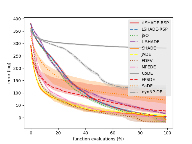
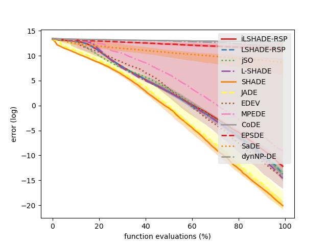
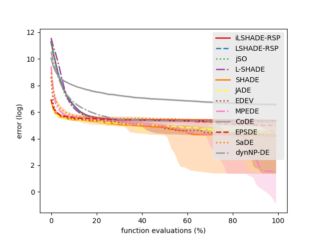
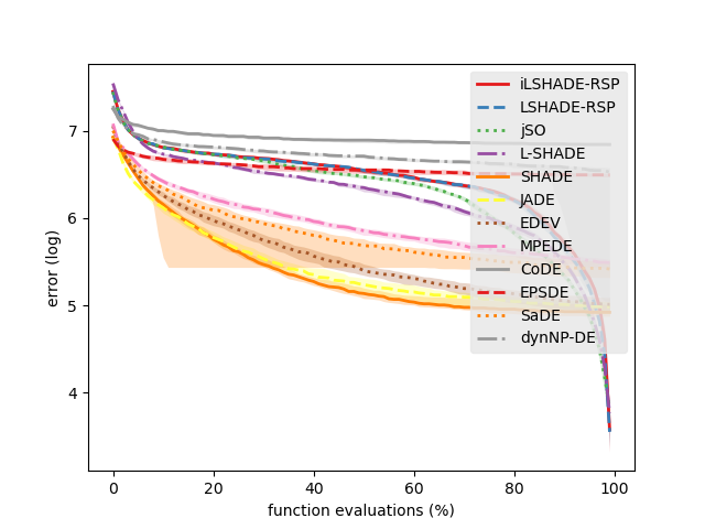
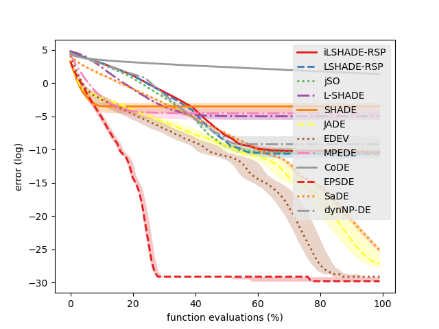
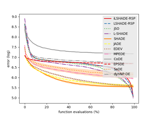
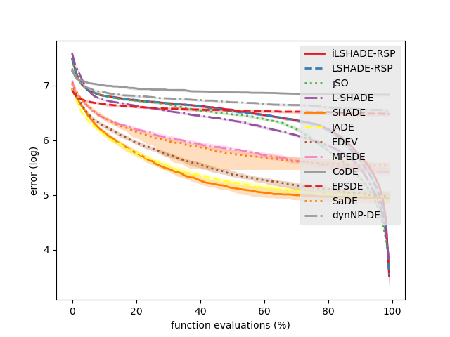
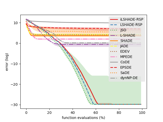
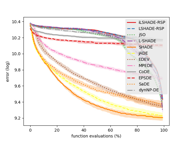
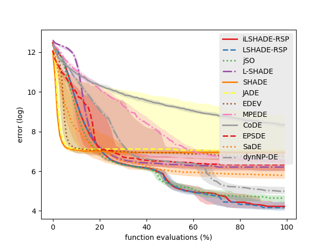
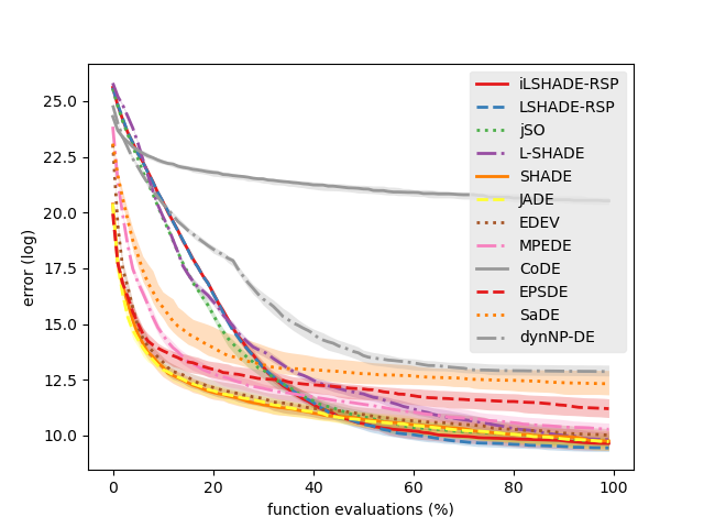
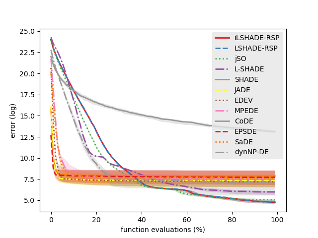
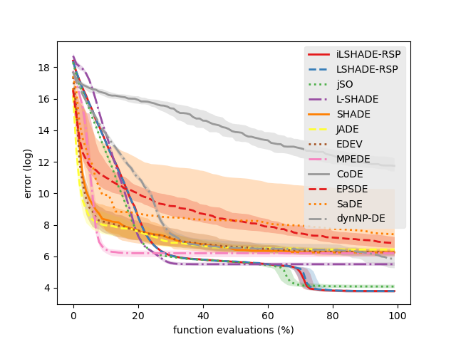
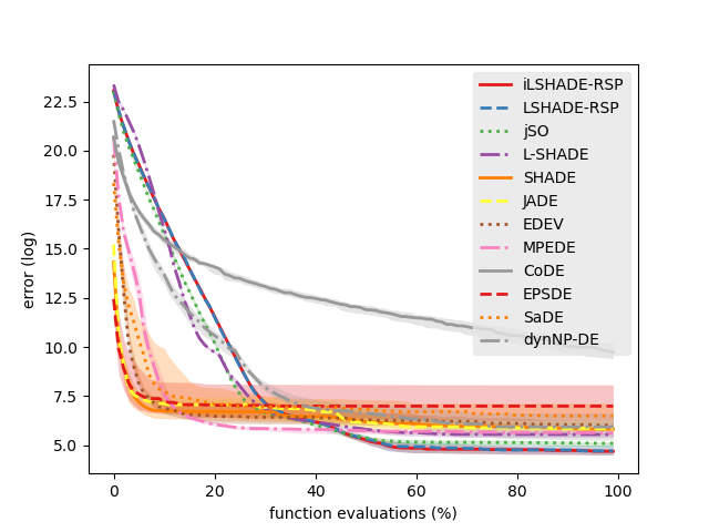
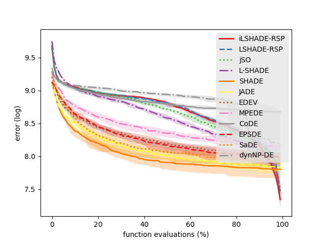
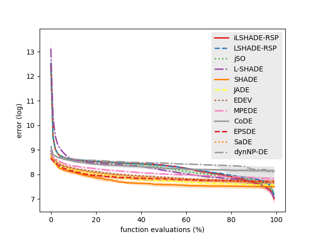
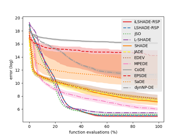
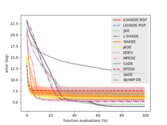
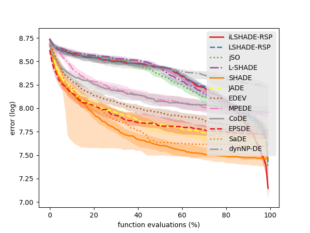
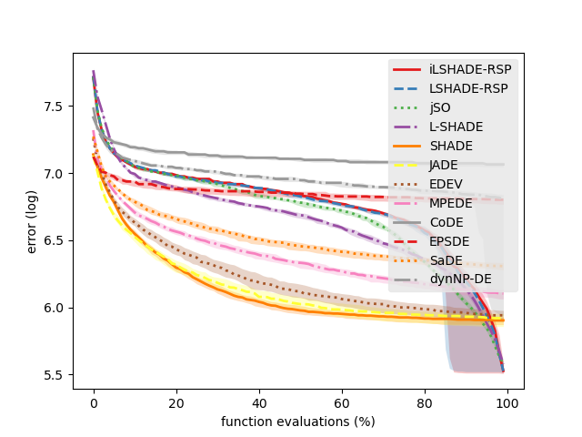
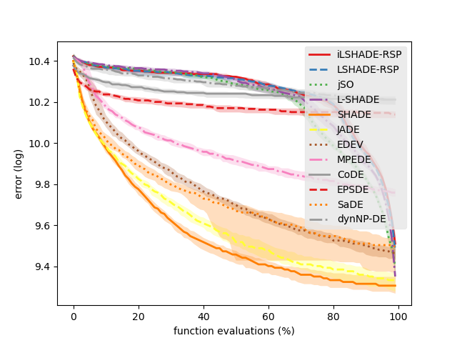
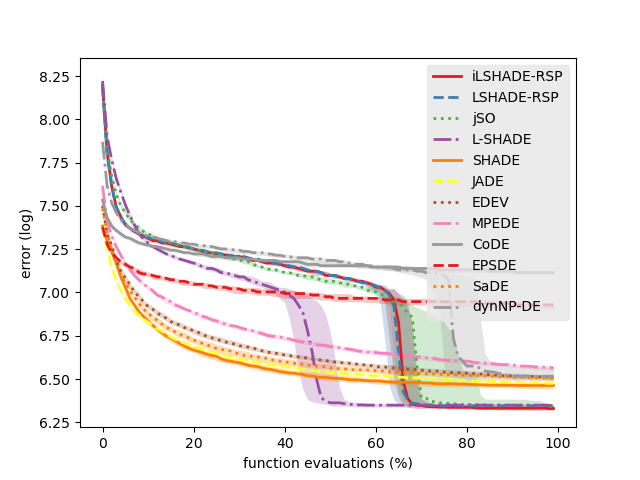
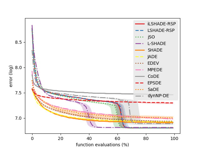
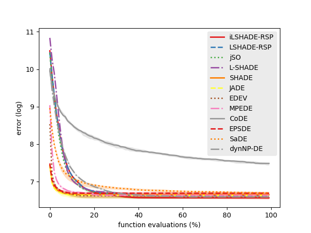
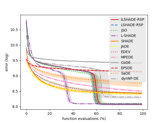
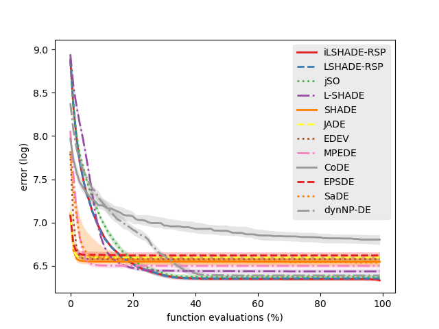
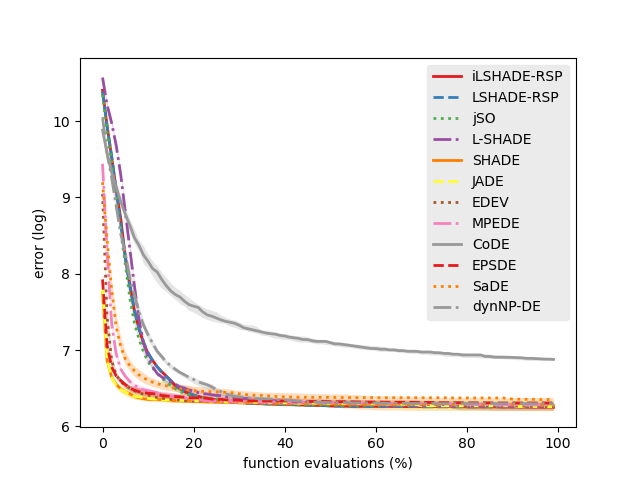
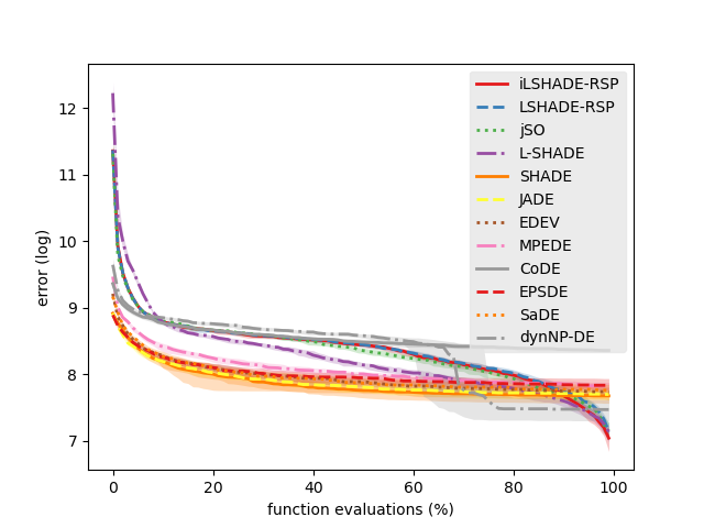
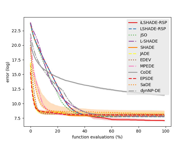
We present the comparative analysis of the test algorithms in this subsection. Tables 1, 3, 5, and 7 present the means and standard deviations of the FEVs of the test algorithms in 10, 30, 50, and 100 dimension, respectively. In the tables, the symbols “+”, “=”, and “-” denote that the corresponding algorithm has statistically better, similar or worse performance compared to the proposed algorithm, respectively. Moreover, Tables 2, 4, 6, and 8 present the results of the Friedman test with Hochberg’s post hoc in 10, 30, 50, and 100 dimension, respectively. Furthermore, Figs. 3, 4, 5, 6, and 7 provide the convergence graphs of the test algorithms in 100 dimension.
Table 1 presents the means and standard deviations of the FEVs of the test algorithms in 10 dimension, obtained by 51 independent runs. As can be seen from the table, the proposed algorithm performs better performance than all of the other test algorithms. Specifically, iLSHADE-RSP found significantly better solutions with lower FEVs than SHADE, JADE, EDEV, MPEDE, CoDE, EPSDE, and SaDE on more than 50 percent of the test functions. In particular, MPEDE and CoDE were significantly outperformed by iLSHADE-RSP on approximately 80 percent of the test functions. As compared to its predecessor LSHADE-RSP, the proposed algorithm considerably outperformed on 2 test functions and underperformed it on 0 test functions. In addition, Table 2 presents the Friedman test with Hochberg’s post hoc, which supports the comparative analysis in Table 1 where iLSHADE-RSP ranked the first among the test algorithms, and the outperformance over JADE, EDEV, MPEDE, CoDE, EPSDE, and SaDE was statistically significant.
The means and standard deviations of the FEVs of the proposed and comparison algorithms in 30 dimension are shown in Table 3, collected by 51 independent runs. As can be seen from the table, the proposed algorithm performs better performance than all of the other test algorithms. Specifically, iLSHADE-RSP found significantly better solutions with lower FEVs than SHADE, JADE, EDEV, MPEDE, CoDE, EPSDE, SaDE, and dynNP-DE on more than 80 percent of the test functions. In particular, JADE, EDEV, MPEDE, CoDE, EPSDE, and SaDE were not able to outperform iLSHADE-RSP on any of the test functions. As compared to its predecessor LSHADE-RSP, the proposed algorithm considerably outperformed on 6 test functions and underperformed it on 1 test functions. Additionally, Table 4 presents the Friedman test with Hochberg’s post hoc, which supports the comparative analysis in Table 3 where iLSHADE-RSP ranked the first among the test algorithms, and the outperformance over SHADE, JADE, EDEV, MPEDE, CoDE, EPSDE, SaDE, and dynNP-DE was statistically significant.
Table 5 presents the means and standard deviations of the FEVs of the test algorithms in 50 dimension, obtained by 51 independent runs. As can be seen from the table, the proposed algorithm performs better performance than all of the other test algorithms. Specifically, iLSHADE-RSP found significantly better solutions with lower FEVs than all of the other test algorithms except LSHADE-RSP on more than 50 percent of the test functions. In particular, SHADE, JADE, EDEV, MPEDE, CoDE, EPSDE, SaDE, and dynNP-DE were significantly outperformed by iLSHADE-RSP on approximately 90 percent of the test functions. As compared to its predecessor LSHADE-RSP, the proposed algorithm considerably outperformed on 8 test functions and underperformed it on 4 test functions. In addition, Table 6 presents the Friedman test with Hochberg’s post hoc, which supports the comparative analysis in Table 5 where iLSHADE-RSP ranked the first among the test algorithms, and the outperformance over SHADE, JADE, EDEV, MPEDE, CoDE, EPSDE, SaDE, and dynNP-DE was statistically significant.
The means and standard deviations of the FEVs of the proposed and comparison algorithms in 100 dimension are shown in Table 7, collected by 51 independent runs. As can be seen from the table, the proposed algorithm performs better performance than all of the other test algorithms. Specifically, iLSHADE-RSP found significantly better solutions with lower FEVs than all of the other test algorithms except LSHADE-RSP on more than 50 percent of the test functions. In particular, MPEDE, CoDE, EPSDE, SaDE, and dynNP-DE were significantly outperformed by iLSHADE-RSP on approximately 90 percent of the test functions. As compared to its predecessor LSHADE-RSP, the proposed algorithm considerably outperformed on 8 test functions and underperformed it on 5 test functions. Additionally, Table 8 presents the Friedman test with Hochberg’s post hoc, which supports the comparative analysis in Table 7 where iLSHADE-RSP ranked the first among the test algorithms, and the outperformance over SHADE, JADE, EDEV, MPEDE, CoDE, EPSDE, SaDE, and dynNP-DE was statistically significant.
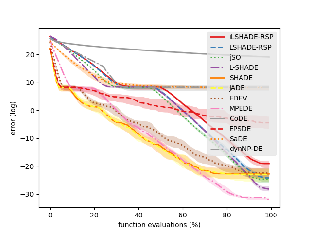
The convergence graphs of the proposed and comparison algorithms in 100 dimension are provided in Figs 3, 4, 5, 6, and 7. Each convergence graph provides the median and interquartile ranges (one-fourth and three-fourth) of the FEVs of the proposed and comparison algorithms. The first part of the convergence graphs ( - ) is given in Fig. 3. The second part of the convergence graphs ( - ) is given in Fig. 4. The third part of the convergence graphs ( - ) is given in Fig. 5. The fourth part of the convergence graphs ( - ) is given in Fig. 6. The last part of the convergence graphs ( - ) is given in Fig. 7. As can be seen from the figures, iLSHADE-RSP is competitive with the other test algorithms in terms of solution accuracy, especially for the test functions , - , - , and - . In particular, iLSHADE-RSP can escape from the local optimum of the test functions and , while the other test algorithms cannot.
6.2 Discussion of Comparative Analysis
We first discuss the comparative analysis between the proposed algorithm and each of the two state-of-the-art L-SHADE variants, LSHADE-RSP and jSO. After that, we discuss the experimental results with the proposed algorithm and the other test algorithms.
-
1.
The performance difference between the proposed algorithm and LSHADE-RSP is negligible in 10 dimension. The proposed algorithm has only two improvements against zero deteriorations. However, the performance difference is much different in 30, 50, and 100 dimensions. The proposed algorithm has six improvements against one deterioration in 30 dimension, eight improvements against four deteriorations in 50 dimension, and eight improvements against five deteriorations in 100 dimension. Additionally, we investigated the performance difference with respect to the characteristics of the test functions. We found out that the proposed algorithm has worse performance on the unimodal (-) and some of the simple multimodal test functions (-) but better performance on the expanded multimodal (-) and the hybrid composition test functions (-). In a word, the proposed algorithm performs better than LSHADE-RSP on more complicated optimization problems.
-
2.
The performance difference between the proposed algorithm and jSO is negligible in 10 dimension. The proposed algorithm has only five improvements against three deteriorations. However, the performance difference is much different in 30, 50, and 100 dimensions. The proposed algorithm has 11 improvements against six deteriorations in 30 dimension, 17 improvements against two deteriorations in 50 dimension, and 18 improvements against six deteriorations in 100 dimension. Additionally, we investigated the performance difference with respect to the characteristics of the test functions. We found out that the proposed algorithm has worse performance on the unimodal (-) and some of the simple multimodal test functions (-) but better performance on the expanded multimodal (-) and the hybrid composition test functions (-). In a word, the proposed algorithm performs better than jSO on more complicated optimization problems.
-
3.
The proposed algorithm found more significantly accurate solutions compared with the test algorithms, including L-SHADE, SHADE, JADE, EDEV, MPEDE, CoDE, EPSDE, SaDE, and dynNP-DE, in all the dimensions.
Note that, the experimental results with the proposed algorithm and LSHADE-RSP lend weight to the effectiveness of the modified recombination operator of the proposed algorithm, which can increase the probability of finding an optimal solution by adopting the long-tailed property of the Cauchy distribution, and thus, it can improve the optimization performance of LSHADE-RSP significantly.
| iLSHADE-RSP | ||||||||
|---|---|---|---|---|---|---|---|---|
| MEAN (STD DEV) | MEAN (STD DEV) | MEAN (STD DEV) | MEAN (STD DEV) | MEAN (STD DEV) | MEAN (STD DEV) | MEAN (STD DEV) | MEAN (STD DEV) | |
| F1 | 2.26E-14 (1.99E-14) | 1.56E-14 (6.51E-15) + | 1.61E-14 (6.36E-15) = | 1.98E-14 (2.12E-14) = | 2.65E-14 (3.32E-14) = | 2.92E-14 (2.82E-14) = | 3.90E-14 (4.52E-14) - | 6.05E-14 (9.22E-14) - |
| F2 | 8.13E-14 (2.21E-13) | 4.29E-14 (5.25E-14) = | 3.85E-13 (2.17E-12) = | 6.35E-14 (1.48E-13) = | 7.47E-14 (1.33E-13) = | 1.55E-13 (6.30E-13) = | 5.52E-14 (7.29E-14) = | 1.27E-13 (2.28E-13) = |
| F3 | 2.01E-13 (8.60E-14) | 1.39E-13 (4.14E-14) + | 1.66E-13 (5.98E-14) + | 1.73E-13 (5.43E-14) = | 2.47E-13 (9.49E-14) - | 2.91E-13 (1.24E-13) - | 4.28E-13 (1.84E-13) - | 4.87E-13 (2.28E-13) - |
| F4 | 6.83E+01 (5.32E+01) | 5.61E+01 (4.73E+01) = | 5.45E+01 (5.10E+01) = | 6.55E+01 (5.32E+01) = | 5.62E+01 (5.03E+01) + | 6.04E+01 (5.20E+01) + | 7.08E+01 (5.44E+01) + | 5.54E+01 (4.96E+01) + |
| F5 | 1.51E+01 (5.06E+00) | 1.50E+01 (3.86E+00) = | 1.49E+01 (3.78E+00) = | 1.52E+01 (4.47E+00) = | 1.56E+01 (4.96E+00) = | 1.60E+01 (5.66E+00) = | 1.53E+01 (5.10E+00) = | 1.65E+01 (5.35E+00) = |
| F6 | 9.98E-07 (1.80E-06) | 2.61E-07 (5.54E-07) + | 3.93E-07 (5.74E-07) = | 5.26E-07 (9.13E-07) = | 7.25E-07 (1.27E-06) = | 1.22E-06 (1.53E-06) - | 2.11E-06 (3.76E-06) - | 3.62E-06 (3.35E-06) - |
| F7 | 7.25E+01 (7.22E+00) | 6.96E+01 (5.97E+00) + | 7.15E+01 (5.70E+00) = | 7.11E+01 (6.27E+00) = | 7.37E+01 (8.33E+00) = | 7.55E+01 (7.89E+00) = | 7.63E+01 (9.80E+00) = | 7.60E+01 (1.00E+01) = |
| F8 | 1.62E+01 (4.46E+00) | 1.64E+01 (5.05E+00) = | 1.55E+01 (3.86E+00) = | 1.56E+01 (5.44E+00) = | 1.74E+01 (5.45E+00) = | 1.74E+01 (5.56E+00) = | 1.67E+01 (5.28E+00) = | 1.66E+01 (4.91E+00) = |
| F9 | 4.25E-14 (5.57E-14) | 6.71E-15 (2.71E-14) + | 2.24E-14 (4.57E-14) = | 2.24E-14 (4.57E-14) = | 3.58E-14 (5.34E-14) = | 4.69E-14 (5.67E-14) = | 4.47E-14 (5.62E-14) = | 5.81E-14 (5.76E-14) = |
| F10 | 4.23E+03 (5.00E+02) | 4.13E+03 (5.09E+02) = | 4.18E+03 (6.67E+02) = | 4.24E+03 (6.18E+02) = | 4.25E+03 (6.39E+02) = | 4.19E+03 (6.33E+02) = | 4.20E+03 (5.26E+02) = | 4.13E+03 (5.96E+02) = |
| F11 | 1.77E+01 (3.42E+00) | 1.97E+01 (4.26E+00) - | 1.75E+01 (3.65E+00) = | 1.74E+01 (4.07E+00) = | 1.82E+01 (3.28E+00) = | 1.87E+01 (2.67E+00) = | 1.82E+01 (2.74E+00) = | 1.89E+01 (2.76E+00) - |
| F12 | 1.42E+03 (4.59E+02) | 1.55E+03 (4.16E+02) = | 1.45E+03 (4.04E+02) = | 1.43E+03 (4.25E+02) = | 1.43E+03 (4.15E+02) = | 1.47E+03 (4.64E+02) = | 1.39E+03 (3.50E+02) = | 1.41E+03 (3.96E+02) = |
| F13 | 3.03E+01 (2.09E+01) | 2.38E+01 (1.68E+01) = | 2.91E+01 (2.44E+01) = | 2.90E+01 (2.34E+01) = | 2.99E+01 (2.42E+01) = | 2.83E+01 (1.93E+01) = | 3.09E+01 (1.73E+01) = | 3.03E+01 (1.91E+01) = |
| F14 | 2.36E+01 (1.88E+00) | 2.40E+01 (2.17E+00) = | 2.40E+01 (2.02E+00) = | 2.33E+01 (2.07E+00) = | 2.36E+01 (2.09E+00) = | 2.34E+01 (2.00E+00) = | 2.36E+01 (1.82E+00) = | 2.34E+01 (1.76E+00) = |
| F15 | 1.87E+01 (1.89E+00) | 1.91E+01 (1.86E+00) = | 1.97E+01 (1.61E+00) - | 1.88E+01 (1.63E+00) = | 1.88E+01 (2.48E+00) = | 1.83E+01 (1.72E+00) = | 1.84E+01 (2.14E+00) = | 1.84E+01 (1.71E+00) = |
| F16 | 2.94E+02 (1.29E+02) | 3.04E+02 (1.39E+02) = | 3.15E+02 (1.28E+02) = | 3.19E+02 (1.37E+02) = | 3.03E+02 (1.12E+02) = | 3.20E+02 (1.18E+02) = | 3.48E+02 (1.32E+02) - | 3.35E+02 (1.16E+02) - |
| F17 | 2.27E+02 (8.62E+01) | 2.34E+02 (9.75E+01) = | 2.42E+02 (1.06E+02) = | 2.47E+02 (9.24E+01) = | 2.29E+02 (8.94E+01) = | 2.30E+02 (8.92E+01) = | 2.36E+02 (1.06E+02) = | 2.47E+02 (9.12E+01) = |
| F18 | 2.26E+01 (1.27E+00) | 2.27E+01 (1.27E+00) = | 2.29E+01 (1.41E+00) = | 2.27E+01 (1.18E+00) = | 2.30E+01 (1.46E+00) = | 2.27E+01 (1.49E+00) = | 2.25E+01 (1.32E+00) = | 2.26E+01 (1.40E+00) = |
| F19 | 1.03E+01 (2.46E+00) | 1.13E+01 (2.01E+00) - | 1.06E+01 (2.31E+00) = | 1.04E+01 (2.85E+00) = | 1.06E+01 (2.12E+00) = | 1.10E+01 (2.26E+00) = | 1.07E+01 (2.43E+00) = | 1.10E+01 (2.35E+00) = |
| F20 | 1.18E+02 (4.79E+01) | 1.40E+02 (7.51E+01) = | 1.18E+02 (5.10E+01) = | 1.17E+02 (2.78E+01) = | 1.17E+02 (4.85E+01) = | 1.27E+02 (4.78E+01) = | 1.23E+02 (4.14E+01) = | 1.35E+02 (5.64E+01) - |
| F21 | 2.15E+02 (4.35E+00) | 2.15E+02 (4.13E+00) = | 2.15E+02 (3.70E+00) = | 2.16E+02 (5.24E+00) = | 2.16E+02 (4.93E+00) = | 2.17E+02 (5.49E+00) = | 2.15E+02 (5.17E+00) = | 2.17E+02 (4.96E+00) = |
| F22 | 1.86E+03 (2.25E+03) | 1.91E+03 (2.21E+03) = | 1.58E+03 (2.22E+03) = | 1.51E+03 (2.13E+03) = | 1.86E+03 (2.25E+03) = | 1.31E+03 (2.01E+03) = | 1.70E+03 (2.13E+03) = | 1.62E+03 (2.14E+03) = |
| F23 | 4.33E+02 (7.17E+00) | 4.31E+02 (5.46E+00) = | 4.33E+02 (6.28E+00) = | 4.33E+02 (7.21E+00) = | 4.32E+02 (6.43E+00) = | 4.32E+02 (6.17E+00) = | 4.33E+02 (6.92E+00) = | 4.33E+02 (6.58E+00) = |
| F24 | 5.09E+02 (4.10E+00) | 5.08E+02 (3.48E+00) = | 5.09E+02 (4.42E+00) = | 5.09E+02 (3.67E+00) = | 5.10E+02 (4.09E+00) = | 5.10E+02 (4.15E+00) = | 5.10E+02 (4.31E+00) = | 5.09E+02 (3.48E+00) = |
| F25 | 4.79E+02 (9.87E-01) | 4.80E+02 (1.41E+00) - | 4.80E+02 (7.77E-01) - | 4.80E+02 (8.57E-01) = | 4.79E+02 (8.08E-01) = | 4.79E+02 (9.61E-01) = | 4.79E+02 (9.51E-01) = | 4.79E+02 (7.84E-01) + |
| F26 | 1.13E+03 (4.73E+01) | 1.15E+03 (5.73E+01) = | 1.13E+03 (5.44E+01) = | 1.14E+03 (5.75E+01) = | 1.13E+03 (5.27E+01) = | 1.12E+03 (5.25E+01) + | 1.13E+03 (5.84E+01) = | 1.13E+03 (5.18E+01) = |
| F27 | 4.77E+02 (6.46E+00) | 4.89E+02 (9.29E+00) - | 4.83E+02 (9.11E+00) - | 4.78E+02 (5.88E+00) = | 4.79E+02 (7.93E+00) = | 4.75E+02 (5.64E+00) = | 4.74E+02 (5.90E+00) + | 4.74E+02 (8.15E+00) + |
| F28 | 4.52E+02 (3.37E-01) | 4.53E+02 (6.69E-01) - | 4.53E+02 (5.94E-01) - | 4.52E+02 (3.82E-01) = | 4.52E+02 (4.81E+00) = | 4.52E+02 (4.76E-01) + | 4.52E+02 (4.76E-01) + | 4.51E+02 (4.93E-01) + |
| F29 | 3.06E+02 (1.93E+01) | 3.28E+02 (3.69E+01) - | 3.17E+02 (2.52E+01) - | 3.12E+02 (2.03E+01) = | 3.04E+02 (2.04E+01) = | 2.99E+02 (1.75E+01) + | 3.01E+02 (1.84E+01) = | 2.99E+02 (1.61E+01) + |
| F30 | 4.19E+03 (5.95E+03) | 1.76E+04 (4.90E+04) - | 3.97E+03 (6.15E+03) = | 2.79E+03 (3.05E+03) = | 2.68E+03 (2.65E+03) = | 3.79E+03 (3.31E+03) = | 6.32E+03 (7.45E+03) = | 6.26E+03 (6.91E+03) - |
| +/=/- | 5/18/7 | 1/24/5 | 0/30/0 | 1/28/1 | 4/24/2 | 3/23/4 | 5/18/7 |
The symbols “+/=/-” indicate that the corresponding algorithm performed significantly better (), not significantly better or worse (), or significantly worse () compared to iLSHADE-RSP with using the Wilcoxon rank-sum test with significance level.
| iLSHADE-RSP | ||||||||
|---|---|---|---|---|---|---|---|---|
| MEAN (STD DEV) | MEAN (STD DEV) | MEAN (STD DEV) | MEAN (STD DEV) | MEAN (STD DEV) | MEAN (STD DEV) | MEAN (STD DEV) | MEAN (STD DEV) | |
| F1 | 2.03E-14 (1.43E-14) | 2.09E-14 (1.25E-14) = | 2.09E-14 (1.37E-14) = | 2.03E-14 (8.64E-15) = | 1.73E-14 (6.55E-15) = | 2.12E-14 (1.28E-14) = | 2.17E-14 (1.62E-14) = | 1.92E-14 (1.23E-14) = |
| F2 | 6.18E-14 (1.07E-13) | 4.21E-11 (3.00E-10) = | 1.29E-13 (6.31E-13) = | 1.67E-13 (7.37E-13) = | 1.25E-13 (3.92E-13) = | 4.51E-14 (9.51E-14) = | 1.59E-13 (5.81E-13) = | 4.46E-14 (4.84E-14) = |
| F3 | 2.29E-13 (6.66E-14) | 2.17E-13 (7.92E-14) = | 1.95E-13 (6.63E-14) + | 2.15E-13 (1.00E-13) = | 1.86E-13 (6.32E-14) + | 2.01E-13 (5.92E-14) + | 2.20E-13 (6.41E-14) = | 1.94E-13 (6.01E-14) + |
| F4 | 5.93E+01 (5.19E+01) | 7.70E+01 (5.40E+01) - | 6.12E+01 (5.24E+01) - | 6.44E+01 (5.28E+01) - | 5.09E+01 (4.67E+01) + | 6.34E+01 (5.08E+01) = | 7.00E+01 (5.30E+01) = | 5.28E+01 (4.87E+01) = |
| F5 | 1.50E+01 (5.08E+00) | 1.55E+01 (4.26E+00) = | 1.57E+01 (5.91E+00) = | 1.69E+01 (3.98E+00) - | 1.48E+01 (4.27E+00) = | 1.46E+01 (4.74E+00) = | 1.36E+01 (3.66E+00) = | 1.52E+01 (4.07E+00) = |
| F6 | 4.24E-07 (5.09E-07) | 4.60E-07 (6.69E-07) = | 5.48E-07 (8.21E-07) = | 7.05E-07 (1.02E-06) = | 5.25E-07 (7.93E-07) = | 6.85E-07 (1.32E-06) = | 4.05E-07 (4.82E-07) = | 7.64E-07 (1.27E-06) = |
| F7 | 7.33E+01 (8.29E+00) | 7.45E+01 (8.12E+00) = | 7.21E+01 (7.05E+00) = | 7.42E+01 (9.08E+00) = | 7.35E+01 (6.44E+00) = | 7.14E+01 (7.06E+00) = | 7.17E+01 (6.10E+00) = | 7.08E+01 (5.93E+00) = |
| F8 | 1.57E+01 (4.72E+00) | 1.61E+01 (4.59E+00) = | 1.57E+01 (5.85E+00) = | 1.74E+01 (5.91E+00) = | 1.53E+01 (4.67E+00) = | 1.43E+01 (4.37E+00) = | 1.46E+01 (4.78E+00) = | 1.54E+01 (3.97E+00) = |
| F9 | 4.02E-14 (5.50E-14) | 2.68E-14 (4.88E-14) = | 4.02E-14 (5.50E-14) = | 3.58E-14 (5.34E-14) = | 3.58E-14 (5.34E-14) = | 2.24E-14 (4.57E-14) = | 1.79E-14 (4.19E-14) = | 2.68E-14 (4.88E-14) = |
| F10 | 4.19E+03 (6.37E+02) | 4.66E+03 (6.18E+02) - | 4.55E+03 (6.74E+02) - | 4.34E+03 (5.03E+02) = | 3.92E+03 (6.17E+02) + | 3.81E+03 (6.12E+02) + | 3.94E+03 (5.35E+02) + | 3.74E+03 (6.22E+02) + |
| F11 | 1.84E+01 (3.32E+00) | 1.91E+01 (4.69E+00) = | 2.01E+01 (4.16E+00) - | 1.83E+01 (3.70E+00) = | 1.82E+01 (3.70E+00) = | 1.96E+01 (3.99E+00) = | 1.99E+01 (4.17E+00) = | 2.20E+01 (3.91E+00) - |
| F12 | 1.41E+03 (3.66E+02) | 1.08E+03 (3.01E+02) + | 1.26E+03 (4.28E+02) + | 1.45E+03 (4.26E+02) = | 1.44E+03 (3.63E+02) = | 1.54E+03 (3.89E+02) = | 1.57E+03 (3.42E+02) - | 1.32E+03 (3.84E+02) = |
| F13 | 2.49E+01 (1.69E+01) | 2.75E+01 (2.14E+01) = | 3.04E+01 (1.91E+01) = | 2.58E+01 (1.63E+01) = | 2.86E+01 (2.39E+01) = | 2.47E+01 (1.85E+01) = | 2.97E+01 (2.10E+01) = | 3.26E+01 (1.87E+01) - |
| F14 | 2.42E+01 (2.59E+00) | 2.37E+01 (2.06E+00) = | 2.45E+01 (1.95E+00) = | 2.37E+01 (2.22E+00) = | 2.36E+01 (1.95E+00) = | 2.36E+01 (1.93E+00) = | 2.36E+01 (2.21E+00) = | 2.34E+01 (1.99E+00) = |
| F15 | 1.80E+01 (1.55E+00) | 1.86E+01 (1.92E+00) = | 1.83E+01 (1.73E+00) = | 1.80E+01 (1.99E+00) = | 1.93E+01 (1.93E+00) - | 1.97E+01 (2.06E+00) - | 2.06E+01 (2.30E+00) - | 2.06E+01 (1.84E+00) - |
| F16 | 3.58E+02 (1.49E+02) | 3.37E+02 (1.49E+02) = | 3.48E+02 (1.26E+02) = | 3.10E+02 (1.28E+02) = | 3.22E+02 (1.42E+02) = | 3.03E+02 (1.14E+02) + | 3.16E+02 (1.28E+02) = | 3.20E+02 (9.99E+01) = |
| F17 | 2.59E+02 (1.06E+02) | 2.82E+02 (1.39E+02) = | 2.92E+02 (1.30E+02) = | 2.53E+02 (7.98E+01) = | 2.26E+02 (9.65E+01) = | 2.21E+02 (8.00E+01) = | 2.18E+02 (8.77E+01) + | 2.24E+02 (7.52E+01) = |
| F18 | 2.27E+01 (1.32E+00) | 2.29E+01 (1.49E+00) = | 2.30E+01 (1.37E+00) = | 2.28E+01 (1.40E+00) = | 2.29E+01 (1.71E+00) = | 2.27E+01 (1.40E+00) = | 2.32E+01 (1.36E+00) = | 2.25E+01 (1.04E+00) = |
| F19 | 1.04E+01 (2.15E+00) | 9.22E+00 (2.37E+00) + | 9.61E+00 (1.80E+00) = | 1.02E+01 (1.96E+00) = | 1.05E+01 (2.00E+00) = | 1.15E+01 (2.67E+00) = | 1.08E+01 (2.42E+00) = | 1.06E+01 (2.72E+00) = |
| F20 | 1.18E+02 (3.65E+01) | 1.88E+02 (1.17E+02) - | 1.53E+02 (6.84E+01) - | 1.34E+02 (7.27E+01) = | 1.06E+02 (3.39E+01) + | 1.14E+02 (3.91E+01) = | 1.11E+02 (3.58E+01) = | 1.01E+02 (1.78E+01) + |
| F21 | 2.15E+02 (5.23E+00) | 2.16E+02 (4.81E+00) = | 2.17E+02 (5.51E+00) = | 2.16E+02 (4.97E+00) = | 2.15E+02 (4.61E+00) = | 2.16E+02 (4.24E+00) = | 2.15E+02 (4.74E+00) = | 2.14E+02 (4.27E+00) = |
| F22 | 1.65E+03 (2.15E+03) | 1.73E+03 (2.34E+03) = | 1.61E+03 (2.18E+03) = | 1.74E+03 (2.28E+03) = | 1.80E+03 (2.24E+03) = | 1.37E+03 (2.00E+03) = | 1.24E+03 (1.91E+03) = | 1.08E+03 (1.83E+03) = |
| F23 | 4.34E+02 (6.62E+00) | 4.34E+02 (7.70E+00) = | 4.33E+02 (7.11E+00) = | 4.31E+02 (8.02E+00) = | 4.31E+02 (6.21E+00) + | 4.31E+02 (6.96E+00) = | 4.30E+02 (6.45E+00) + | 4.31E+02 (7.17E+00) = |
| F24 | 5.09E+02 (3.67E+00) | 5.09E+02 (4.60E+00) = | 5.09E+02 (3.73E+00) = | 5.09E+02 (4.74E+00) = | 5.08E+02 (3.49E+00) = | 5.09E+02 (3.75E+00) = | 5.10E+02 (3.62E+00) = | 5.09E+02 (3.63E+00) = |
| F25 | 4.80E+02 (1.20E+00) | 4.80E+02 (1.83E+00) - | 4.80E+02 (1.48E+00) - | 4.79E+02 (9.18E-01) = | 4.79E+02 (1.10E+00) = | 4.79E+02 (6.66E-01) = | 4.80E+02 (7.00E-01) - | 4.80E+02 (7.84E-01) - |
| F26 | 1.12E+03 (4.92E+01) | 1.14E+03 (5.97E+01) = | 1.13E+03 (5.17E+01) = | 1.13E+03 (4.77E+01) = | 1.13E+03 (5.25E+01) = | 1.13E+03 (4.12E+01) = | 1.13E+03 (6.13E+01) = | 1.13E+03 (5.02E+01) = |
| F27 | 4.79E+02 (6.08E+00) | 5.00E+02 (0.00E+00) - | 5.00E+02 (0.00E+00) - | 4.86E+02 (1.02E+01) - | 5.03E+02 (1.17E+01) - | 5.08E+02 (9.27E+00) - | 5.11E+02 (1.19E+01) - | 5.10E+02 (8.80E+00) - |
| F28 | 4.52E+02 (2.44E-01) | 4.99E+02 (5.23E-01) - | 4.97E+02 (1.89E+00) - | 4.52E+02 (5.05E-01) - | 4.52E+02 (3.25E-01) = | 4.52E+02 (3.11E-01) = | 4.53E+02 (4.40E-01) - | 4.54E+02 (6.70E+00) - |
| F29 | 3.15E+02 (2.82E+01) | 3.03E+02 (1.85E+01) + | 2.92E+02 (1.35E+01) + | 2.98E+02 (1.70E+01) + | 3.75E+02 (1.95E+01) - | 3.70E+02 (1.78E+01) - | 3.73E+02 (1.70E+01) - | 3.71E+02 (2.10E+01) - |
| F30 | 4.06E+03 (4.03E+03) | 5.75E+02 (1.42E+02) + | 1.05E+03 (3.43E+02) + | 3.93E+03 (2.93E+03) = | 4.08E+05 (5.34E+04) - | 5.54E+05 (5.52E+04) - | 5.89E+05 (3.07E+04) - | 5.98E+05 (2.60E+04) - |
| +/=/- | 4/20/6 | 4/19/7 | 1/25/4 | 5/21/4 | 3/23/4 | 3/20/7 | 3/19/8 |
The symbols “+/=/-” indicate that the corresponding algorithm performed significantly better (), not significantly better or worse (), or significantly worse () compared to iLSHADE-RSP with using the Wilcoxon rank-sum test with significance level.
6.3 Analysis of iLSHADE-RSP
6.3.1 Parameter Values for Jumping Rate
As we mentioned earlier, the proposed algorithm alternately applies one of the two recombination operators according to the jumping rate . The jumping rate determines the additional exploration of the proposed algorithm. If the jumping rate is too high, the modified recombination operator is applied too often, and thus, the proposed algorithm might not be beneficial from existing candidate solutions. On the other hand, if the jumping rate is too low, the modified recombination operator is applied too rarely, and thus, the additional exploration of the proposed algorithm might be negligible. We carried out experiments to find out appropriate parameter values for the jumping rate. Table 9 shows the means and standard deviations of the FEVs of the proposed algorithm with different parameter values for the jumping rate. As can be seen from the table, the parameter values can lead to satisfactory results.
6.3.2 Lévy Perturbation
As we mentioned earlier, the proposed algorithm employs a modified recombination operator, which calculates a perturbation of a target vector with the Cauchy distribution. The Cauchy distribution is a special case of the Lévy -stable distribution. Therefore, it is interesting to test the other cases of the Lévy -stable distribution for the modified recombination operator. The Lévy -stable distribution can be defined by the characteristic function, derived by Lévy [65] and Hall [66] as follows.
| (19) |
where
| (20) |
The Lévy -stable distribution denoted by has four parameters: the stability parameter , the skewness parameter , the scale parameter , and the location parameter . The Lévy -stable distribution has three special cases as follows.
-
1.
The Gaussian distribution: .
-
2.
The Cauchy distribution: .
-
3.
The Lévy distribution: .
The modified recombination operator, which calculates a perturbation of a target vector with the Lévy -stable distribution can be defined as follows.
| (21) |
We used Chambers-Mallows-Stuck method [67, 68, 69, 70] to generate Lévy -stable random numbers as follows.
Step 1. Generate a random number from the uniform distribution and a random number from the exponential distribution with mean 1.
Step 2. If then:
(22) where
(23)
(24)
Step 3. If then:
(25)
Step 4. If then:
(26) is .
Table 10 shows the means and standard deviations of the FEVs of the proposed algorithm with different stability parameters for the Lévy -stable distribution with the jumping rate . For simplicity’s sake, we only considered symmetric distributions. The Lévy -stable distribution has a short and wide PDF if the stability parameter is high, while a tall and narrow PDF if the stability parameter is low. As can be seen from the table, the parameter values can lead to satisfactory results. In other words, the modified recombination operator with from the Cauchy distribution () to the Lévy -stable distribution () works best for the proposed algorithm. We chose the Cauchy distribution for the modified recombination operator because generating Cauchy random numbers is much easier than generating Lévy -stable random numbers.
7 Conclusion
Differential evolution is a popular evolutionary algorithm for multidimensional real-valued functions. Like other evolutionary algorithms, it is important for differential evolution to establish a balance between exploration and exploitation to be successful. Recently, a state-of-the-art DE variant called LSHADE-RSP was proposed. Although it has shown excellent performance, the greediness of LSHADE-RSP may cause premature convergence in which all the candidate solutions fall into the local optimum of an optimization problem and cannot escape from there.
To mitigate the problem, we have devised a modified recombination operator for LSHADE-RSP, which perturbs a target vector with the Cauchy distribution. Therefore, the modified recombination operator can increase the probability of finding an optimal solution by adopting the long-tailed property of the Cauchy distribution. We called the resulting algorithm iLSHADE-RSP, which alternately applies the original and modified recombination operators according to a jumping rate.
The proposed algorithm has been tested on the CEC 2017 test suite in 10, 30, 50, and 100 dimensions. Our experimental results verify that the improved LSHADE-RSP significantly outperformed not only its predecessor LSHADE-RSP but also several cutting-edge DE variants in terms of convergence speed and solution accuracy. In particular, the proposed algorithm performs better than the comparison algorithms on more complicated optimization problems, such as expanded multimodal test functions and hybrid composition test functions, in all the dimensions.
Possible directions for future work include 1) testing the proposed algorithm for constrained optimization problems; 2) testing the proposed algorithm for large-scale optimization problems; 3) applying the proposed algorithm to various real-world problems.
Acknowledgement
This work was supported by the National Research Foundation of Korea(NRF) grant funded by the Korea government(MSIT) (No. NRF-2017R1C1B2012752). The correspondence should be addressed to Dr. Chang Wook Ahn.
References
- [1] M. Črepinšek, S.-H. Liu, M. Mernik, Exploration and exploitation in evolutionary algorithms: A survey, ACM computing surveys (CSUR) 45 (3) (2013) 1–33.
- [2] A. E. Eiben, C. A. Schippers, On evolutionary exploration and exploitation, Fundamenta Informaticae 35 (1-4) (1998) 35–50.
- [3] R. Storn, K. Price, Differential evolution–a simple and efficient heuristic for global optimization over continuous spaces, Journal of global optimization 11 (4) (1997) 341–359.
- [4] K. Price, R. M. Storn, J. A. Lampinen, Differential evolution: a practical approach to global optimization, Springer Science & Business Media, 2006.
- [5] S. Das, P. N. Suganthan, Differential evolution: A survey of the state-of-the-art, IEEE transactions on evolutionary computation 15 (1) (2010) 4–31.
- [6] S. Das, S. S. Mullick, P. N. Suganthan, Recent advances in differential evolution–an updated survey, Swarm and Evolutionary Computation 27 (2016) 1–30.
- [7] J. Zhang, A. C. Sanderson, JADE: adaptive differential evolution with optional external archive, IEEE Transactions on evolutionary computation 13 (5) (2009) 945–958.
- [8] R. Tanabe, A. Fukunaga, Success-history based parameter adaptation for differential evolution, in: 2013 IEEE congress on evolutionary computation, IEEE, 2013, pp. 71–78.
- [9] R. Tanabe, A. S. Fukunaga, Improving the search performance of shade using linear population size reduction, in: 2014 IEEE congress on evolutionary computation (CEC), IEEE, 2014, pp. 1658–1665.
- [10] J. Brest, M. S. Maučec, B. Bošković, iL-SHADE: Improved L-SHADE algorithm for single objective real-parameter optimization, in: 2016 IEEE Congress on Evolutionary Computation (CEC), IEEE, 2016, pp. 1188–1195.
- [11] J. Brest, M. S. Maučec, B. Bošković, Single objective real-parameter optimization: algorithm jSO, in: 2017 IEEE congress on evolutionary computation (CEC), IEEE, 2017, pp. 1311–1318.
- [12] N. H. Awad, M. Z. Ali, P. N. Suganthan, R. G. Reynolds, An ensemble sinusoidal parameter adaptation incorporated with L-SHADE for solving CEC2014 benchmark problems, in: 2016 IEEE congress on evolutionary computation (CEC), IEEE, 2016, pp. 2958–2965.
- [13] N. H. Awad, M. Z. Ali, P. N. Suganthan, R. G. Reynolds, A. M. Shatnawi, A novel differential crossover strategy based on covariance matrix learning with Euclidean neighborhood for solving real-world problems, in: 2017 IEEE Congress on Evolutionary Computation (CEC), IEEE, 2017, pp. 380–386.
- [14] N. H. Awad, M. Z. Ali, P. N. Suganthan, Ensemble sinusoidal differential covariance matrix adaptation with Euclidean neighborhood for solving CEC2017 benchmark problems, in: 2017 IEEE Congress on Evolutionary Computation (CEC), IEEE, 2017, pp. 372–379.
- [15] N. H. Awad, M. Z. Ali, P. N. Suganthan, Ensemble of parameters in a sinusoidal differential evolution with niching-based population reduction, Swarm and evolutionary computation 39 (2018) 141–156.
- [16] A. W. Mohamed, A. A. Hadi, A. M. Fattouh, K. M. Jambi, LSHADE with semi-parameter adaptation hybrid with CMA-ES for solving CEC 2017 benchmark problems, in: 2017 IEEE Congress on evolutionary computation (CEC), IEEE, 2017, pp. 145–152.
- [17] V. Stanovov, S. Akhmedova, E. Semenkin, LSHADE algorithm with rank-based selective pressure strategy for solving CEC 2017 benchmark problems, in: 2018 IEEE Congress on Evolutionary Computation (CEC), IEEE, 2018, pp. 1–8.
- [18] J.-F. Yeh, T.-Y. Chen, T.-C. Chiang, Modified L-SHADE for single objective real-parameter optimization, in: 2019 IEEE Congress on Evolutionary Computation (CEC), IEEE, 2019, pp. 381–386.
- [19] J. E. Baker, Adaptive selection methods for genetic algorithms, in: Proceedings of an International Conference on Genetic Algorithms and their applications, Hillsdale, New Jersey, 1985, pp. 101–111.
- [20] K. A. De Jong, Analysis of the behavior of a class of genetic adaptive systems, Tech. rep. (1975).
- [21] S. J. Louis, G. J. Rawlins, Syntactic analysis of convergence in genetic algorithms, in: Foundations of genetic algorithms, Vol. 2, Elsevier, 1993, pp. 141–151.
- [22] D. E. Goldberg, P. Segrest, Finite markov chain analysis of genetic algorithms, in: Proceedings of the second international conference on genetic algorithms, Vol. 1, 1987, p. 1.
- [23] T. J. Choi, J. Togelius, Y.-G. Cheong, Advanced Cauchy mutation for differential evolution in numerical optimization, IEEE Access 8 (2020) 8720–8734.
- [24] T. J. Choi, J. Togelius, Y.-G. Cheong, ACM-DE: Adaptive p-best Cauchy mutation with linear failure threshold reduction for differential evolution in numerical optimization, arXiv preprint arXiv:1907.01095.
- [25] H. Zhang, X. Lei, C. Wang, D. Yue, X. Xie, Adaptive grid based multi-objective Cauchy differential evolution for stochastic dynamic economic emission dispatch with wind power uncertainty, PloS one 12 (9).
- [26] M. Ali, M. Pant, Improving the performance of differential evolution algorithm using Cauchy mutation, Soft Computing 15 (5) (2011) 991–1007.
- [27] H. Qin, J. Zhou, Y. Lu, Y. Wang, Y. Zhang, Multi-objective differential evolution with adaptive Cauchy mutation for short-term multi-objective optimal hydro-thermal scheduling, Energy Conversion and Management 51 (4) (2010) 788–794.
- [28] N. Awad, M. Ali, J. Liang, B. Qu, P. Suganthan, Problem definitions and evaluation criteria for the CEC 2017 special session and competition on single objective real-parameter numerical optimization, Tech. Rep.
- [29] J. Brest, S. Greiner, B. Boskovic, M. Mernik, V. Zumer, Self-adapting control parameters in differential evolution: A comparative study on numerical benchmark problems, IEEE transactions on evolutionary computation 10 (6) (2006) 646–657.
- [30] J. Brest, M. S. Maučec, Population size reduction for the differential evolution algorithm, Applied Intelligence 29 (3) (2008) 228–247.
- [31] T. J. Choi, C. W. Ahn, J. An, An adaptive Cauchy differential evolution algorithm for global numerical optimization, The Scientific World Journal 2013.
- [32] M. Leon, N. Xiong, Adapting differential evolution algorithms for continuous optimization via greedy adjustment of control parameters, Journal of Artificial Intelligence and Soft Computing Research 6 (2) (2016) 103–118.
- [33] T. J. Choi, C. W. Ahn, An improved differential evolution algorithm and its application to large-scale artificial neural networks, in: Journal of Physics: Conference Series, Vol. 806, IOP Publishing, 2017, p. 012010.
- [34] T. J. Choi, C. W. Ahn, Adaptive -stable differential evolution in numerical optimization, Natural Computing 16 (4) (2017) 637–657.
- [35] P. Bujok, J. Tvrdík, Enhanced individual-dependent differential evolution with population size adaptation, in: 2017 IEEE congress on evolutionary computation (CEC), IEEE, 2017, pp. 1358–1365.
- [36] T. J. Choi, Y. Lee, Asynchronous differential evolution with self-adaptive parameter control for global numerical optimization, in: MATEC Web of Conferences, Vol. 189, EDP Sciences, 2018, p. 03020.
- [37] T. J. Choi, Y.-G. Cheong, C. W. Ahn, A performance comparison of crossover variations in differential evolution for training multi-layer perceptron neural networks, in: International Conference on Bio-Inspired Computing: Theories and Applications, Springer, 2018, pp. 477–488.
- [38] A. K. Qin, V. L. Huang, P. N. Suganthan, Differential evolution algorithm with strategy adaptation for global numerical optimization, IEEE transactions on Evolutionary Computation 13 (2) (2008) 398–417.
- [39] R. Mallipeddi, P. N. Suganthan, Q.-K. Pan, M. F. Tasgetiren, Differential evolution algorithm with ensemble of parameters and mutation strategies, Applied soft computing 11 (2) (2011) 1679–1696.
- [40] Y. Wang, Z. Cai, Q. Zhang, Differential evolution with composite trial vector generation strategies and control parameters, IEEE transactions on evolutionary computation 15 (1) (2011) 55–66.
- [41] T. J. Choi, C. W. Ahn, An adaptive Cauchy differential evolution algorithm with bias strategy adaptation mechanism for global numerical optimization., JCP 9 (9) (2014) 2139–2145.
- [42] T. J. Choi, C. W. Ahn, An adaptive differential evolution algorithm with automatic population resizing for global numerical optimization, in: Bio-Inspired Computing-Theories and Applications, Springer, 2014, pp. 68–72.
- [43] T. J. Choi, C. W. Ahn, An adaptive population resizing scheme for differential evolution in numerical optimization, Journal of Computational and Theoretical Nanoscience 12 (7) (2015) 1336–1350.
- [44] T. J. Choi, C. W. Ahn, An adaptive Cauchy differential evolution algorithm with population size reduction and modified multiple mutation strategies, in: Proceedings of the 18th Asia Pacific Symposium on Intelligent and Evolutionary Systems-Volume 2, Springer, 2015, pp. 13–26.
- [45] G. Wu, R. Mallipeddi, P. N. Suganthan, R. Wang, H. Chen, Differential evolution with multi-population based ensemble of mutation strategies, Information Sciences 329 (2016) 329–345.
- [46] G. Wu, X. Shen, H. Li, H. Chen, A. Lin, P. N. Suganthan, Ensemble of differential evolution variants, Information Sciences 423 (2018) 172–186.
- [47] T. J. Choi, C. W. Ahn, Adaptive Cauchy differential evolution with strategy adaptation and its application to training large-scale artificial neural networks, in: International Conference on Bio-Inspired Computing: Theories and Applications, Springer, 2017, pp. 502–510.
- [48] T. J. Choi, Y. Lee, Asynchronous differential evolution with strategy adaptation for global numerical optimization, in: Proceedings of the 2018 2nd High Performance Computing and Cluster Technologies Conference, 2018, pp. 15–18.
- [49] S. Rahnamayan, H. R. Tizhoosh, M. M. Salama, Opposition-based differential evolution, IEEE Transactions on Evolutionary computation 12 (1) (2008) 64–79.
- [50] H. Wang, Z. Wu, S. Rahnamayan, Enhanced opposition-based differential evolution for solving high-dimensional continuous optimization problems, Soft Computing 15 (11) (2011) 2127–2140.
- [51] S.-Y. Park, J.-J. Lee, Stochastic opposition-based learning using a beta distribution in differential evolution, IEEE transactions on cybernetics 46 (10) (2015) 2184–2194.
- [52] T. J. Choi, J. Togelius, Y.-G. Cheong, A fast and efficient stochastic opposition-based learning for differential evolution in numerical optimization, arXiv preprint arXiv:1908.08011.
- [53] T. J. Choi, J.-H. Lee, H. Y. Youn, C. W. Ahn, Adaptive differential evolution with elite opposition-based learning and its application to training artificial neural networks, Fundamenta Informaticae 164 (2-3) (2019) 227–242.
- [54] E. Mininno, F. Neri, F. Cupertino, D. Naso, Compact differential evolution, IEEE Transactions on Evolutionary Computation 15 (1) (2010) 32–54.
- [55] J.-h. Zhong, J. Zhang, SDE: a stochastic coding differential evolution for global optimization, in: Proceedings of the 14th annual conference on Genetic and evolutionary computation, 2012, pp. 975–982.
- [56] H. Wang, S. Rahnamayan, H. Sun, M. G. Omran, Gaussian bare-bones differential evolution, IEEE Transactions on Cybernetics 43 (2) (2013) 634–647.
- [57] R. D. Al-Dabbagh, F. Neri, N. Idris, M. S. Baba, Algorithmic design issues in adaptive differential evolution schemes: Review and taxonomy, Swarm and Evolutionary Computation 43 (2018) 284–311.
- [58] K. R. Opara, J. Arabas, Differential evolution: A survey of theoretical analyses, Swarm and evolutionary computation 44 (2019) 546–558.
- [59] I. C. Trelea, The particle swarm optimization algorithm: convergence analysis and parameter selection, Information processing letters 85 (6) (2003) 317–325.
- [60] T. Liao, T. Stuetzle, Benchmark results for a simple hybrid algorithm on the CEC 2013 benchmark set for real-parameter optimization, in: 2013 IEEE Congress on Evolutionary Computation, IEEE, 2013, pp. 1938–1944.
- [61] B. Lacroix, D. Molina, F. Herrera, Dynamically updated region based memetic algorithm for the 2013 CEC special session and competition on real parameter single objective optimization, in: 2013 IEEE Congress on Evolutionary Computation, IEEE, 2013, pp. 1945–1951.
- [62] N. Hansen, The CMA evolution strategy: a comparing review, in: Towards a new evolutionary computation, Springer, 2006, pp. 75–102.
- [63] W. Gong, Z. Cai, Differential evolution with ranking-based mutation operators, IEEE Transactions on Cybernetics 43 (6) (2013) 2066–2081.
- [64] J. Demšar, Statistical comparisons of classifiers over multiple data sets, Journal of Machine learning research 7 (Jan) (2006) 1–30.
- [65] P. Lévy, Sur les intégrales dont les éléments sont des variables aléatoires indépendantes, Annali della Scuola Normale Superiore di Pisa-Classe di Scienze 3 (3-4) (1934) 337–366.
- [66] P. Hall, A comedy of errors: the canonical form for a stable characteristic function, Bulletin of the London Mathematical Society 13 (1) (1981) 23–27.
- [67] J. M. Chambers, C. L. Mallows, B. Stuck, A method for simulating stable random variables, Journal of the american statistical association 71 (354) (1976) 340–344.
- [68] R. Weron, On the Chambers-Mallows-Stuck method for simulating skewed stable random variables, Statistics & Probability Letters 28 (2) (1996) 165–171.
- [69] R. Weron, et al., Correction to:” on the Chambers–Mallows–Stuck method for simulating skewed stable random variables”, Tech. rep., University Library of Munich, Germany (2010).
- [70] R. Weron, Computationally intensive value at risk calculations, Tech. rep., Papers/Humboldt-Universität Berlin, Center for Applied Statistics and … (2004).