Technical Report

Fast multipole methods for the evaluation of layer potentials with locally-corrected quadratures

Leslie Greengard
Courant Institute, NYU 2in Center for Computational Mathematics, Flatiron Institute
New York, NY, 10012 2in New York, NY 10010
greengard@cims.nyu.edu

Michael O’Neil
Courant Institute, NYU
New York, NY 10012
oneil@cims.nyu.edu

Manas Rachh
Center for Computational Mathematics, Flatiron Institute
New York, NY 10010
mrachh@flatironinstitute.org

Felipe Vico
Instituto de Telecomunicaciones y Aplicaciones Multimedia (ITEAM)
Universidad Polit‘ecnica de Valencia
Valencia, Spain 46022
felipe.vico@gmail.com

Abstract

While fast multipole methods (FMMs) are in widespread use for the rapid evaluation of potential fields governed by the Laplace, Helmholtz, Maxwell or Stokes equations, their coupling to high-order quadratures for evaluating layer potentials is still an area of active research. In three dimensions, a number of issues need to be addressed, including the specification of the surface as the union of high-order patches, the incorporation of accurate quadrature rules for integrating singular or weakly singular Green’s functions on such patches, and their coupling to the oct-tree data structures on which the FMM separates near and far field interactions. Although the latter is straightforward for point distributions, the near field for a patch is determined by its physical dimensions, not the distribution of discretization points on the surface.

Here, we present a general framework for efficiently coupling locally corrected quadratures with FMMs, relying primarily on what are called generalized Gaussian quadratures rules, supplemented by adaptive integration. The approach, however, is quite general and easily applicable to other schemes, such as Quadrature by Expansion (QBX). We also introduce a number of accelerations to reduce the cost of quadrature generation itself, and present several numerical examples of acoustic scattering that demonstrate the accuracy, robustness, and computational efficiency of the scheme. On a single core of an Intel i5 2.3GHz processor, a Fortran implementation of the scheme can generate near field quadrature corrections for between 1000 and 10,000 points per second, depending on the order of accuracy and the desired precision. A Fortran implementation of the algorithm described in this work is available at https://gitlab.com/fastalgorithms/fmm3dbie.

Keywords: Nyström method, Helmholtz, quadrature, fast multipole method.

1 Introduction

Over the last two decades, fast multipole methods (FMMs) and related hierarchical fast algorithms have become widespread for computing $N$-body interactions in computational chemistry, astrophysics, acoustics, fluid dynamics, and electromagnetics. In the time-harmonic, acoustic setting, a typical computation of interest is the evaluation of

$$F_{m}=\sum_{\begin{subarray}{c}n=1\\ n\neq m\end{subarray}}^{N}\sigma_{n}\,G_{k}(\bm{x}_{m},\bm{x}_{n})$$ (1.1)

where

$$G_{k}(\bm{x},\bm{y})=\frac{e^{ik|\bm{x}-\bm{y}|}}{4\pi|\bm{x}-\bm{y}|}$$ (1.2)

is the free-space Green’s function for the Helmholtz equation

$$\Delta u+k^{2}u=0.$$

Direct calculation of Equation 1.1 requires $\mathcal{O}(N^{2})$ operations, while the FMM requires $\mathcal{O}(N)$ work in the low frequency regime [1] and $\mathcal{O}(N\log N)$ work in the high frequency regime [2].

When solving boundary value problems for partial differential equations (PDEs) in three dimensions, such sums arise in the discretization of layer potentials defined on a surface $\Gamma$. These potentials take the form:

$$u(\bm{x})=\int_{\Gamma}K(\bm{x},\bm{x}^{\prime})\,\sigma(\bm{x}^{\prime})\,da(\bm{x}^{\prime}).$$ (1.3)

In (1.3), $K(\bm{x},\bm{x}^{\prime})$ is a Green’s function for the PDE of interest, such as (1.2) or one of its directional derivatives. As a result, the governing equation is automatically satisfied, and it remains only to enforce the desired boundary condition. With a suitable choice for the kernel $K(\bm{x},\bm{x}^{\prime})$, this often leads to a Fredholm integral equation of the form

$$\sigma(\bm{x})+\int_{\Gamma}K(\bm{x},\bm{x}^{\prime})\,\sigma(\bm{x}^{\prime})\,da(\bm{x}^{\prime})=f(\bm{x}),\qquad\text{for }\bm{x}\in\Gamma.$$ (1.4)

As we shall see below, this can be discretized with high-order accuracy using a suitable Nyström method [3, 4]

$$\sigma_{i}+w_{ii}\sigma_{i}+\sum_{j\neq i}w_{ij}\,K(\bm{x}_{i},\bm{x}_{j})\,\sigma_{j}\,=f(\bm{x}_{i}).$$ (1.5)

Here, $\bm{x}_{i}$ and $w_{ij}$ are the quadrature nodes and weights, respectively, while $\sigma_{i}$ is an approximation to the true value $\sigma(\bm{x}_{i})$. If the quadrature weights $w_{ij}$ did not depend on the target location, i.e. $w_{ij}=w_{j}$, then the above sum is a standard $N$-body calculation of the form (1.1).

Unfortunately, when the integral equation comes from a layer potential corresponding to an elliptic PDE, the kernel $K$ is typically singular or weakly singular so that simple high-order rules for smooth functions fail. Assuming the surface $\Gamma$ is defined as the union of many smooth patches $\Gamma_{j}$ (each with its own parameterization), high-order quadrature schemes require an analysis of the distance of the target $\bm{x}_{i}$ from each patch.

More precisely, for a given target location $\bm{x}_{i}$ on the boundary, the integral in (1.3) or (1.4) can be split into three pieces: a self-interaction integral, a near field integral, and a far field integral:

$$\int_{\Gamma}K(\bm{x}_{i},\bm{x}^{\prime})\,\sigma(\bm{x}^{\prime})\,da(\bm{x}^{\prime})=\int_{\text{Self}(\bm{x}_{i})}K(\bm{x}_{i},\bm{x}^{\prime})\,\sigma(\bm{x}^{\prime})\,da(\bm{x}^{\prime})\,+\\ \int_{\text{Near}(\bm{x}_{i})}K(\bm{x}_{i},\bm{x}^{\prime})\,\sigma(\bm{x}^{\prime})\,da(\bm{x}^{\prime})\,+\int_{\text{Far}(\bm{x}_{i})}K(\bm{x}_{i},\bm{x}^{\prime})\,\sigma(\bm{x}^{\prime})\,da(\bm{x}^{\prime}).$$ (1.6)

This splitting into target-dependent regions is essential for maintaining high-order accuracy. The region $\text{Self}(\bm{x}_{i})$ is simply the patch on which $\bm{x}_{i}$ itself lies. The integral over this patch involves a singular integrand (due to the kernel $K$). The Near field is defined precisely in Section 4, but consists of patches close enough to $\bm{x}_{i}$ such that the integrand is nearly singular even though it is formally smooth. The Far region consists of all other patches, sufficiently far from $\bm{x}_{i}$ such that high-order quadratures for smooth functions can be applied.

Definition 1.

Suppose that $\bm{x}_{i}$ is in the far field of a patch $\Gamma_{m}$, and that

$$\sum_{j=1}^{M}w_{j}\,K(\bm{x}_{i},\bm{s}_{j})\,\sigma_{j}\,\approx\int_{\Gamma_{m}}K(\bm{x}_{i},\bm{x}^{\prime})\,\sigma(\bm{x}^{\prime})\,da(\bm{x}^{\prime})$$ (1.7)

to the desired precision. Then $\bm{s}_{j}$ and $w_{j}$ will be referred to as the far field quadrature nodes and weights. Note that these are independent of $\bm{x}_{i}$.

A related task in the solution process is evaluating the computed solution $u(\bm{x})$ at target locations $\bm{x}$ which are off-surface, but possibly arbitrarily close to the surface. In this case as well, while the integrands are formally smooth, evaluating the integral presents a similar challenge owing to the nearly singular behavior of the integrand. The evaluation of the potential can still be split into two pieces in a similar manner: a near field integral and a far field integral

$$\int_{\Gamma}K(\bm{x},\bm{x}^{\prime})\,\sigma(\bm{x}^{\prime})\,da(\bm{x}^{\prime})=\int_{\text{Near}(\bm{x})}K(\bm{x},\bm{x}^{\prime})\,\sigma(\bm{x}^{\prime})\,da(\bm{x}^{\prime})\\ +\int_{\text{Far}(\bm{x})}K(\bm{x},\bm{x}^{\prime})\,\sigma(\bm{x}^{\prime})\,da(\bm{x}^{\prime}).$$ (1.8)

The strategy outlined above can be used for evaluating the contributions of the near and far regions for targets off-surface as well.

While methods exist for the Self and Near calculations, the use of a fast algorithm such as the FMM requires coupling these somewhat complicated quadrature schemes to the Cartesian oct-tree data structures that divide up space into a hierarchy of regular, adaptively refined cubes. Unfortunately, the surface patches $\Gamma_{m}$ of the domain boundary $\Gamma$ may be of vastly different sizes and do not, in general, conform to a spatial subdivision strategy based on the density of quadrature nodes as points in $\mathbb{R}^{3}$. That is, many patches (curvilinear triangles) $\Gamma_{j}$ are likely to cross leaf node boundaries in the oct-tree structure. If this were not the case, then far field interactions within the FMM could be handled by computing multipole expansions from entire patches, followed by direct calculation of the Self and Near quadratures (analogous to the direct, near neighbor calculations in a point-based FMM). Thus, one of the issues we address here concerns modifications of the FMM so that speed is conserved for far field interactions, but in a manner where the overhead for near field quadrature corrections is modest, even when the surface patches are nonuniform.

Furthermore, while we will restrict our attention here to Nyström-style discretizations, the same concerns must be addressed for collocation and Galerkin-type methods. Similar issues arise when coupling adaptive mesh refinement (AMR) data structures to complicated geometries using Cartesian cut-cell methods [5, 6, 7].

In the present paper, we develop an efficient algorithm which allows for the straightforward coupling of adaptive FMM data structures with locally corrected quadrature schemes. Our goal is to achieve $\mathcal{O}(N)$ or $\mathcal{O}(N\log N)$ performance for surfaces with $O(N)$ discretizations points, depending on whether one is in the low or high frequency regime, respectively. Moreover, we would like the constant implicit in this notation to be as close to the performance of point-based FMMs as possible. We will concentrate on the use of generalized Gaussian quadrature rules [8, 9, 10, 11] for the self interactions on curvilinear triangles, and adaptive integration for the Near region (nearly singular interactions). It is, perhaps, surprising that adaptive integration on surface patches can be competitive with other schemes such as Quadrature By Expansion (QBX), singularity subtraction, or coordinate transformations [12, 13, 14, 15, 16, 17, 18, 19]. The key is that we have developed a careful, precision and geometry-dependent hierarchy of interpolators on each patch, after which the adaptive integration step is inexpensive when amortized over all relevant targets. As a side-effect, our scheme also provides rapid access to entries of the fully discretized system matrix which is essential for fast direct solvers.

Remark 1.

Generalized Gaussian quadrature was already coupled to an FMM in [8], but the question of how to design a robust algorithm that is insensitive to large variation in triangle dimensions was not directly addressed. In some sense, the present paper is devoted to two separate issues raised in [8]: the first is to accelerate adaptive quadrature itself, and the second is to describe an FMM implementation that works for multi-scale discretizations.

Remark 2.

It is worth noting that most locally corrected quadrature schemes, such as Duffy transformations [20], are designed for a target that is mapped to the origin of a local coordinate system or the vertex of a triangular patch and, hence, are suitable only for self interactions as defined above. Near interactions are not addressed. An exception is Quadrature by Expansion (QBX) which provides a systematic, uniform procedure for computing layer potentials using only smooth quadratures and extrapolation [21, 16, 17]. These have been successfully coupled to FMMs in [17, 18]. Many aspects of the FMM modifications described here can be used in conjunction with QBX instead. Another exception is Erichsen-Sauter rules [15], which do include schemes for adjacent panels, but appear to be best suited for modest accuracy.

The paper is organized as follows: in Section 2, some basic facts regarding polynomial approximation and integration on triangles are presented. In Section 3, we describe the classical boundary integral equation for acoustic scattering from a sound-soft boundary, governed by the Helmholtz equation, as well as discretization and integration methods for curvilinear surfaces. Section 4 provides the algorithmic details involved in locally corrected quadrature schemes. The coupling of these quadrature schemes to FMMs is presented in Section 5, and numerical examples demonstrating the performance of the scheme are presented in Section 6. Finally, in Section 7, we discuss avenues for further research, and the application of our scheme to fast direct solvers.

2 Interpolation and integration on triangles

For the sake of simplicity, we assume that we are given a surface triangulation represented as a collection of charts $\bm{X}^{j}=\bm{X}^{j}(u,v)$, which map the standard right triangle

$$T_{0}=\{(u,v):u\geq 0\,,v\geq 0\,,u+v\leq 1\}\subset\mathbb{R}^{2}$$ (2.1)

to the surface patch $\Gamma_{j}$. All discretization and integration is done over $T_{0}$, incorporating the mapping function $\bm{X}^{j}$ and its derivatives as needed.

In this section, we summarize the basic polynomial interpolation and integration rules we will use for smooth functions $f:T_{0}\to\mathbb{R}$. A useful spectral basis is given by the orthogonal polynomials on $T_{0}$, known as Koornwinder polynomials [22]. They are described analytically by the formula:

$$K_{nm}(u,v)=c_{nm}\,(1-v)^{m}\,P_{n-m}^{(0,2m+1)}(1-2v)\,P_{m}\left(\frac{2u+v-1}{1-v}\right),\qquad m\leq n,$$ (2.2)

where $P_{n}^{(a,b)}$ is the Jacobi polynomial of degree $n$ with parameters $(a,b)$, $P_{m}$ is the Legendre polynomial of degree $m$, and $c_{nm}$ is a normalization constant such that

$$\int_{T_{0}}|K_{nm}(u,v)|^{2}\,du\,dv=1.$$ (2.3)

For convenience, our definition is slightly different from that in [22].

It is easy to see that there are $n_{p}=p(p+1)/2$ Koornwinder polynomials of total degree less than $p$. By a straightforward change of variables, and using the orthogonality relationships for Legendre and Jacobi polynomials, it is easy to show that

$$\int_{T_{0}}K_{nm}(u,v)\,K_{n^{\prime}m^{\prime}}(u,v)\,du\,dv=0,\qquad\text{for }n\neq n^{\prime}\text{ and }m\neq m^{\prime}.$$ (2.4)

The Koornwinder polynomials form a complete basis for $L^{2}(T_{0})$, and can easily be used to approximate smooth functions on $T_{0}$ to arbitrary precision.

2.1 Polynomial approximation and integration

As in standard spectral approximation methods for functions defined on intervals or tensor products of intervals [23], smooth functions $f$ defined on $T_{0}$ can be interpolated, approximated, and integrated using a Koornwinder polynomial basis.

To this end, suppose that $f$ is defined by a $p$th-order Koornwinder expansion with coefficients $c_{nm}$:

$$f(u,v)=\sum_{n=0}^{p-1}\sum_{m=0}^{n}c_{nm}\,K_{nm}(u,v).$$ (2.5)

Then, the square matrix $\bm{\mathsf{U}}$ that maps the $n_{p}$ coefficients in the above expansion to values of $f$ at a selection of $n_{p}$ interpolation nodes, denoted by $(u_{j},v_{j})\subseteq T_{0}$, has elements

$$\mathsf{U}_{nm,j}=K_{nm}(u_{j},v_{j}).$$ (2.6)

Let the matrix $\bm{\mathsf{V}}=\bm{\mathsf{U}}^{-1}$. Then $\bm{\mathsf{V}}$ maps values of $f$ at the interpolation nodes $(u_{j},v_{j})$ to coefficients in a Koornwinder polynomial expansion.

Suppose now that $f:T_{0}\to\mathbb{R}$ is an arbitrary smooth function (not necessarily a polynomial) and let the values of $f$ at the interpolation points be denoted by $f_{i}=f(u_{i},v_{i})$. Then, a $p$th-order approximation to $f$ is given by

$$f(u,v)\approx\sum_{n=0}^{p-1}\sum_{m=0}^{n}c_{nm}\,K_{nm}(u,v),$$ (2.7)

where

$$c_{nm}=\sum_{j=1}^{n_{p}}\mathsf{V}_{(nm),j}\,f_{j}.$$ (2.8)

We define the conditioning of the interpolation procedure as the condition number of the matrices $\bm{\mathsf{U}}$ or $\bm{\mathsf{V}}$. Much like interpolation operators on the interval, these matrices are not well-conditioned for arbitrary selections of nodes $(u_{j},v_{j})$, as we will briefly discuss in the next two sections.

An $n$-point quadrature rule for computing the integral of a function $f$ on $T_{0}$ is a collection of nodes and weights, $(u_{i},v_{i})$, $w_{i}$, $i=1,2,\ldots n$, such that

$$\int_{T_{0}}f(u,v)\,du\,dv =\int_{0}^{1}\int_{0}^{1-u}f(u,v)\,du\,dv$$ (2.9)

$$\approx\sum_{i=1}^{n}w_{i}\,f_{i},$$

where $f_{i}=f(u_{i},v_{i})$ is the value of $f$ at the $i$th quadrature node. The accuracy of such a quadrature rule is very dependent on the choice of the quadrature nodes; if the rule is to be exact for a selection of $n$ functions, then the values of $w_{i}$ are determined wholly by the selection of $(u_{i},v_{i})$. Since the node selection provides additional degrees of freedom, Gaussian-type quadrature rules are possible. On the triangle, a quadrature rule would be perfectly Gaussian if it integrated $3n$ functions exactly, since there are $3n$ parameters (the two coordinates of the nodes, and the weights). In one dimension, it is well-known that choosing the nodes as the roots of a suitable orthogonal polynomial leads to a perfect Gaussian rule [23]. In two dimensions, such perfect rules do not exist, but approximately Gaussian quadrature rules can be constructed.

2.2 High-order quadrature rules on the simplex $T_{0}$

First described in 2010 [24], what we will refer to as Xiao-Gimbutas quadratures are a set of Gaussian-like rules obtained through the solution of a nonlinear least-squares problem using Newton’s method. The resulting nodes are contained in the interior of $T_{0}$, and all the weights are positive. Various kinds of symmetry can also be specified. For a given $p>0$, these rules are designed to use the minimum number of nodes with positive weights so that the resulting quadrature rule is exact for all polynomials of total degree $<p$. As noted above, there are $n_{p}=p(p+1)/2$ such polynomials. While not perfect Gaussian rules, the Xiao-Gimbutas quadratures achieve remarkably high-order. A rule with 48 weights and nodes, for example, is exact for polynomials of degree 16, of which there are $n_{16}=136$. The rule has only $3\times 48=144$ free parameters.

For the sake of convenience we would like the quadrature nodes to serve as interpolation/approximation nodes as well. There are, however, far fewer Xiao-Gimbutas nodes than functions we would like to interpolate (namely $n_{p}$). Instead of using an even higher order Xiao-Gimbutas rule, with at least $n_{p}$ nodes, we choose an alternative quadrature scheme, introduced by Vioreanu and Rokhlin in 2014 [25]. The Vioreanu-Rokhlin nodes of order $p$, obtained via a similar optimization procedure, are a collection of $n_{p}$ nodes which can be used simultaneously for high-order polynomial interpolation, approximation, and integration on $T_{0}$. We refer the reader to [25] for a thorough discussion. For our purposes, it suffices to note that the interpolation operators computed using these nodes are extremely well-conditioned.

As a quadrature rule, the nodes and weights are Gaussian-like; they have positive weights and integrate more polynomials than there are nodes in the quadrature. For example, the Vioreanu-Rokhlin rule that interpolates polynomials of degree $p=16$, with $n_{16}=136$ nodes, integrates all $378$ polynomials of degree up to $p^{\prime}=27$. A perfect Gaussian rule would integrate $3n_{p}=408$ functions exactly. The relationship between the order of the interpolation scheme $p$ and the order of the quadrature $p^{\prime}$ is somewhat complicated, and obtained empirically [25].

3 Acoustic scattering from a sound-soft boundary

Let $\Omega$ be a bounded region in $\mathbb{R}^{3}$, with smooth boundary $\partial\Omega=\Gamma$. Given a function $f$ defined on $\Gamma$, a function $u$ defined in $\mathbb{R}^{3}\setminus\Omega$ is said to satisfy the exterior Dirichlet problem for the Helmholtz equation if

$$(\Delta+k^{2})\,u =0 \text{in }\mathbb{R}^{3}\setminus\Omega,$$ (3.1)

$$u =f \text{on }\Gamma,$$

$$\lim_{r\to\infty}\,r\left(\frac{\partial u}{\partial r}-iku\right) =0.$$

In acoustics, Dirichlet problems such as this arise when $\partial\Omega$ is sound-soft and $f=-u^{in}$, where $u^{in}$ is an impinging acoustic wave. A standard approach for solving the Dirichlet problem is to let

$$u=\mathcal{D}_{k}[\sigma]-ik\,\mathcal{S}_{k}[\sigma],$$ (3.2)

where $\sigma$ is an unknown density function defined on $\Gamma$. Here $\mathcal{S}$ and $\mathcal{D}$ are the single layer and double layer operators, respectively, given by

$$\mathcal{S}_{k}[\sigma](\bm{x}) =\int_{\Gamma}G_{k}(\bm{x},\bm{y})\,\sigma(\bm{y})\,da(\bm{y}),$$ (3.3)

$$\mathcal{D}_{k}[\sigma](\bm{x}) =\int_{\Gamma}\left(\bm{n}(\bm{y})\cdot\nabla_{\bm{y}}G_{k}(\bm{x},\bm{y})\right)\,\sigma(\bm{y})\,da(\bm{y}),$$ (3.4)

where $\bm{n}(\bm{y})$ is the outward normal at $\bm{y}\in\Gamma$, and $G_{k}(\bm{x},\bm{y})$ is given by (1.2). The representation (3.2) automatically satisfies the Helmholtz equation and the radiation condition in (3.1). Imposing the boundary condition, and using standard jump relations for layer potentials [26], we obtain the following second-kind integral equation along $\Gamma$ for the density $\sigma$:

$$\frac{1}{2}\sigma(\bm{x})+\mathcal{D}_{k}[\sigma](\bm{x})\textendash ik\mathcal{S}_{k}[\sigma](\bm{x})=f(\bm{x}),\qquad\bm{x}\in\Gamma.$$ (3.5)

This involves a slight abuse of notation: for $\bm{x}\in\Gamma$, $\mathcal{D}_{k}[\sigma](\bm{x})$ should be evaluated in the principal value sense.

When solving (3.5), the accurate evaluation of the layer potentials $\mathcal{S}_{k}[\sigma]$, $\mathcal{D}_{k}[\sigma]$ on $\Gamma$ is essential for either direct or iterative solvers. We will focus here on the evaluation of the single layer potential $\mathcal{S}[\sigma]$, assuming $\sigma$ is known. Only minor modifications are needed to address the double layer potential, as well as other scalar or vector-valued layer potentials that arise in electrostatics, elastostatics, viscous flow, or electromagnetics.

3.1 Surface parameterizations

While some simple boundaries (such as spheres, ellipsoids and tori) can be described by global parameterizations, in general it is necessary to describe a complicated surface $\Gamma$ as a collection of surface patches, each of which is referred to as a chart. The collection of charts whose union defines $\Gamma$ will be referred to as an atlas.

More precisely, we assume that the surface is the disjoint union of patches $\Gamma_{j}$

$$\Gamma=\cup_{j=1}^{N_{\textrm{patches}}}\,\Gamma_{j},$$ (3.6)

and that the patch $\Gamma_{j}$ is parameterized by a non-degenerate chart $\bm{X}^{j}:T_{0}\to\Gamma_{j}$, where $T_{0}$ is the standard simplex (2.1). Given these charts $\bm{X}^{j}$, a local coordinate system can be defined on patch $\Gamma_{j}$ by taking its partial derivatives. For this, we define

$$\bm{X}^{j}_{u}\equiv\frac{\partial\bm{X}^{j}}{\partial u},\qquad\bm{X}^{j}_{v}\equiv\frac{\partial\bm{X}^{j}}{\partial v},\qquad\bm{n}^{j}\equiv\bm{X}^{j}_{u}\times\bm{X}^{j}_{v}.$$ (3.7)

Finally, we assume that the triplet $\bm{X}^{j}_{u}$, $\bm{X}^{j}_{v}$, $\bm{n}^{j}$ forms a right-handed coordinate system with $\bm{n}^{j}$ pointing into the unbounded region $\mathbb{R}^{3}\setminus\Omega$. In general, these vectors are neither orthogonal nor of unit length. The area element on the patch $\Gamma_{j}$ is determined by the Jacobian $J^{j}$,

$$da(\bm{X}^{j}) =|\bm{X}^{j}_{u}\times\bm{X}^{j}_{v}|\,du\,dv$$ (3.8)

$$=J^{j}(u,v)\,du\,dv.$$

3.2 Discretization and integration

If $f$ is a function defined on $\Gamma$, then its integral can be decomposed as a sum over patches:

$$\int_{\Gamma}f(\bm{x})\,da(\bm{x}) =\sum_{j=1}^{N_{\textrm{patches}}}\int_{\Gamma_{j}}f(\bm{x})\,da(\bm{x})$$ (3.9)

$$=\sum_{j=1}^{N_{\textrm{patches}}}\int_{T_{0}}f\left(\bm{X}^{j}(u,v)\right)\,J^{j}(u,v)\,dudv$$

$$=\sum_{j=1}^{N_{\textrm{patches}}}\int_{u=0}^{1}\int_{v=0}^{1-u}f\left(\bm{X}^{j}(u,v)\right)\,J^{j}(u,v)\,dudv,$$

where the Jacobian is given in (3.8).

If, in addition, $f$ is smooth, then each of the integrals on $T_{0}$ in (3.9) can be approximated using Xiao-Gimbutas or Vioreanu-Rokhlin quadrature rules, as discussed in Section 2. Using the latter. we have

$$\int_{\Gamma}f(\bm{x})\,da(\bm{x})\approx\sum_{j=1}^{N_{\textrm{patches}}}\sum_{\ell=1}^{n_{p}}w_{\ell}\,f\left(\bm{X}^{j}(u_{\ell},v_{\ell})\right)\,J^{j}(u_{\ell},v_{\ell}),$$ (3.10)

where $n_{p}$ is the number of nodes in the quadrature, which varies depending on the desired order of accuracy.

For a patch $\Gamma_{j}$ and a target $\bm{x}$, however, the integrand appearing in $S_{k}[\sigma](\bm{x})$ is only smooth when $\bm{x}$ is in the far field. When $\bm{x}$ is either on $\Gamma_{j}$ or nearby, we will need to modify our quadrature approach, as described at the outset. Furthermore, in practice, we will only be given approximations of the charts $\bm{X}^{j}$ and the function $f$ (or the density $\sigma$) on each patch to finite order.

In what follows, we define a $p$th-order approximation as one for which the truncation error is $\mathcal{O}(h^{p})$, where $h$ is, say, the diameter of the patch $\Gamma_{j}$. For a scalar function $f$, it can be approximated to $p$th-order in $L^{2}(T_{0})$ using Koornwinder polynomials as

$$f(u,v)\approx\sum_{n+m<p}f_{nm}\,K_{nm}(u,v).$$ (3.11)

The coefficients $f_{nm}$ can be computed using the values-to-coefficients matrix $\bm{\mathsf{V}}$, as described in Section 2.1. The charts $\bm{X}^{j}$ will generally be approximated using a vector version of the above formula:

$$\bm{X}^{j}(u,v) \approx\sum_{n+m<p}\begin{pmatrix}x^{j}_{nm}\\ y^{j}_{nm}\\ z^{j}_{nm}\end{pmatrix}K_{nm}(u,v)$$ (3.12)

$$=\sum_{n+m<p}\bm{x}_{nm}^{j}\,K_{nm}(u,v)$$

It is important to note that even if the charts $\bm{X}^{j}$ are approximated to accuracy $\epsilon$, i.e.

$$\bm{X}^{j}(u,v)=\sum_{n+m<p}\bm{x}_{nm}^{j}\,K_{nm}(u,v)+\mathcal{O}(\epsilon),$$ (3.13)

it does not follow that the Jacobian $J^{j}$ will be evaluated to precision $\epsilon$ as well. The function $J^{j}$ is non-linear and usually requires a higher-order approximation than the individual components of the chart itself. This cannot be avoided unless analytic derivative information is provided for each patch $\Gamma_{j}$. This affects the accuracy of numerical approximations to surface integrals for a fixed set of patches (but not the asymptotic convergence rate).

Remark 3.

In the following, we use the same order of discretization for representing the layer potential densities $\sigma$ and the surface information, i.e. the charts $\bm{X}^{j}$ and their derivatives $\bm{X}^{j}_{u}$, and $\bm{X}^{j}_{v}$. While this choice is made for convenience of notation and software implementation, our approach to evaluating layer potentials extends in a straightforward manner to the case where different orders of discretization are used for representing the surface information and layer potentials densities.

4 Locally corrected quadratures

For a target location $\bm{x}\in\Gamma_{j}$, let us first consider the self interaction

$$\mathcal{S}_{\textrm{Self}}[\sigma](\bm{x})=\int_{\Gamma_{j}}G_{k}(\bm{x},\bm{y})\,\sigma(\bm{y})\,da(\bm{y}).$$ (4.1)

In [8, 9], the authors designed quadrature rules for exactly this purpose, under the assumption that $\sigma$ and $J^{j}$ are well-approximated by polynomials (and therefore representable by Koornwinder expansions). The quadrature schemes in these papers involve a rather intricate set of transformations but yield a set of precomputed tables which, when composed with the chart $\bm{X}^{j}$, yield the desired high-order accuracy. Briefly, for any $\bm{x}\in\Gamma_{j}$, and all $\sigma$ of the form $\sigma(u,v)=\sum_{nm}c_{nm}K_{nm}(u,v)$, there exist $N(\bm{x})$ nodes $(u_{\bm{x},\ell},v_{\bm{x},\ell})\in T_{0}$ and associated quadrature weights $w_{\bm{x},\ell}$, such that

$$\bigg{|}\int_{u=0}^{1}\int_{v=0}^{1-u}G_{k}(\bm{x},\bm{X}^{j}(u,v))\,\sigma(u,v)\,J^{j}(u,v)\,du\,dv\\ -\sum_{\ell=1}^{N(\bm{x})}G_{k}(\bm{x},\bm{X}^{j}(u_{\bm{x},\ell},v_{\bm{x},\ell}))\,\sigma(u_{\bm{x},\ell},v_{\bm{x},\ell})\,J^{j}(u_{\bm{x},\ell},v_{\bm{x},\ell})w_{\bm{x},\ell}\bigg{|}\leq\varepsilon\cdot\|\sigma\|_{\mathbb{L}^{2}(\Gamma_{j})}.$$ (4.2)

As mentioned in the introduction, in the original paper [8], which was focused on quadrature design, a simple coupling to FMMs was mentioned that relied on the underlying discretization being uniformly high-order. Near field interactions were done using on-the-fly adaptive integration. In their subsequent paper [9], this type of expensive adaptive integration was used for all non-self interactions (i.e. no FMM-type acceleration was used at all). Such an approach cannot be directly accelerated with standard FMMs since the effective quadrature weights are functions of both the source and target locations.

Recall that for $\bm{x}\in\mathbb{R}\setminus\Gamma$, we split the single layer potential $\mathcal{S}_{k}[\sigma](\bm{x})$ into two pieces:

$$\mathcal{S}_{k}[\sigma](\bm{x}) =\int_{\Gamma}G_{k}(\bm{x},\bm{y})\,\sigma(\bm{y})\,da(\bm{y})$$ (4.3)

$$=\sum_{\ell=1}^{N_{\textrm{patches}}}\int_{\Gamma_{\ell}}G_{k}(\bm{x},\bm{y})\,\sigma(\bm{y})\,da(\bm{y})=\mathcal{S}_{\textrm{Near}}[\sigma](\bm{x})+\mathcal{S}_{\textrm{Far}}[\sigma](\bm{x})\,,$$

and when $\bm{x}$ lies on the boundary, say on patch $\Gamma_{j}$, then the single layer potential $\mathcal{S}[\sigma](\bm{x})$ is split into three pieces:

$$\mathcal{S}_{k}[\sigma](\bm{x})=\mathcal{S}_{\textrm{Self}}[\sigma](\bm{x})+\mathcal{S}_{\textrm{Near}}[\sigma](\bm{x})+\mathcal{S}_{\textrm{Far}}[\sigma](\bm{x}),$$ (4.4)

where $\mathcal{S}_{\textrm{Self}}[\sigma](\bm{x})$ is defined in (4.1), and the near and far regions associated with a target and the corresponding definitions of $\mathcal{S}_{\textrm{Near}}[\sigma](\bm{x})$ and $\mathcal{S}_{\textrm{Far}}[\sigma](\bm{x})$ are described below.

For this, it turns out to be easier to first take the point of view of a patch rather than a target. Let $\bm{c}_{j}$ denote the centroid of the patch $\Gamma_{j}$,

$$\bm{c}_{j} =\int_{\Gamma_{j}}\bm{x}\,da(\bm{x})$$ (4.5)

$$=\int_{T_{0}}\bm{X}^{j}(u,v)\,du\,dv,$$

and let

$$R_{j}=\min_{R>0}\{R\mid\,\Gamma_{j}\subset B_{R}(\bm{c}_{j})\},$$ (4.6)

where $B_{R}(\bm{c}_{j})$ is the ball of radius $R$ centered at $\bm{c}_{j}$. That is, $B_{R_{j}}(\bm{c}_{j})$ is the ball of minimal radius containing the patch $\Gamma_{j}$. Letting $\eta>1$ be a free parameter for the moment, we define the near field of the patch $\Gamma_{j}$, denoted by $N_{\eta}(\Gamma_{j})$, to be the set of points that do not lie on $\Gamma_{j}$ but are within the ball $B_{\eta R_{j}}(\bm{c}_{j})$ (see Fig. 1). Thus,

$$N_{\eta}(\Gamma_{j})=\{\bm{x}\in\mathbb{R}^{3}\setminus\Gamma_{j}\mid\,d(\bm{c}_{j},\bm{x})\leq\eta R_{j}\}\,.$$ (4.7)

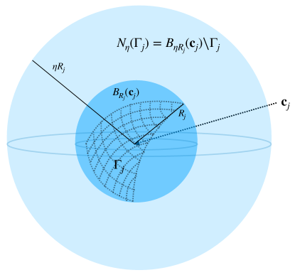
Figure 1: The smallest sphere containing surface patch $\Gamma_{j}$ centered at ${\bf c}_{j}$ and the near field region $N_{\eta}(\Gamma_{j})$. $\eta>1$ is a free parameter whose selection is based on the order of accuracy of the far field quadrature.

Given the collection of near field regions of the form $N_{\eta}(\Gamma_{j})$, let $T_{\eta}(\bm{x})$ denote the dual list: that is, the collection of patches $\Gamma_{j}$ for which the point $\bm{x}\in N_{\eta}(\Gamma_{j})$,

$$T_{\eta}(\bm{x})=\{\Gamma_{j}\mid\bm{x}\in N_{\eta}(\Gamma_{j})\}.$$ (4.8)

Similarly, for $\bm{x}\in\mathbb{R}^{3}\setminus\Gamma$, we denote the far field of $\bm{x}$ by

$$F_{\eta}(\bm{x})=\{\Gamma_{j}\mid\bm{x}\notin N_{\eta}(\Gamma_{j})\}.$$ (4.9)

When $\bm{x}\in\Gamma_{i}$ is a boundary point, we let

$$F_{\eta}(\bm{x})=\{\Gamma_{j},j\neq i\mid\bm{x}\notin N_{\eta}(\Gamma_{j})\}.$$ (4.10)

Then referring to the near-far split of the layer potential for targets off and on-surface described in Equation 4.3, and Equation 4.4, respectively, the near and far part of the layer potentials $\mathcal{S}_{\textrm{Near}}$, and $\mathcal{S}_{\textrm{Far}}$ are given by

$$\mathcal{S}_{\textrm{Near}}[\sigma](\bm{x})=\sum_{\Gamma_{\ell}\in T_{\eta}(\bm{x})}\int_{\Gamma_{\ell}}G_{k}(\bm{x},\bm{y})\,\sigma(\bm{y})\,da(\bm{y})$$ (4.11)

and

$$\mathcal{S}_{\textrm{Far}}[\sigma](\bm{x})=\sum_{\Gamma_{\ell}\in F_{\eta}(\bm{x})}\int_{\Gamma_{\ell}}G_{k}(\bm{x},\bm{y})\,\sigma(\bm{y})\,da(\bm{y}).$$ (4.12)

As noted in the beginning of the section, $\mathcal{S}_{\textrm{Self}}[\sigma](\bm{x})$ can be computed using the generalized Gaussian quadratures of [8, 9]. By virtue of their separation from the source patches, all of the integrands in $\mathcal{S}_{\textrm{Far}}$ are smooth and can be computed using either Vioreanu-Rokhlin or Xiao-Gimbutas quadrature rules, with weights that are independent of the target location $\bm{x}$. The accuracy of these rules, which is affected by the free parameter $\eta$, is discussed in Section 4.1.

It remains only to develop an efficient scheme for evaluating the integrals which define $\mathcal{S}_{\textrm{Near}}[\sigma]$. At present, there do not exist quadrature rules that are capable of simultaneously accounting for the singularity in the Green’s function and the local geometric variation in an efficient manner. The approach developed below involves a judicious combination of precomputation and a greedy, adaptive algorithm applied, for every target point $\bm{x}$, to each $\Gamma_{\ell}\in T_{\eta}(\bm{x})$. Once the near field quadratures have been computed, they can be saved using only $O(N)$ storage. When solving an integral equation iteratively, this can be used to accelerate subsequent applications of the integral operator.

Remark 4.

The evaluation of near field quadratures does not affect the overall complexity of computing layer potentials, assuming $\eta$ is not too large. This follows from the fact that, for each target $\bm{x}$, there are only $O(1)$ patches contained in $T_{\eta}(\bm{x})$. Thus, the cost of all near field contributions is of the order $O(N)$. Since there can be several patches in the near field, however, this computation tends to be the rate limiting step in the overall quadrature generation procedure.

Remark 5.

Without entering into a detailed literature review, it should be noted that coordinate transformation methods such as those in [12, 14, 15, 19] can also be used for computing near field interactions for surface targets. However, these methods don’t apply easily to off-surface evaluation. An alternative to our procedure is Quadrature by Expansion (QBX) [21, 16, 17, 18], which handles singular and nearly-singular integrals in a unified manner and (like the method of this paper) works both on and off surface. There are distinct trade-offs to be made in QBX-based schemes and the scheme presented here. In the end, the best method will be determined by accuracy, efficiency and ease of use. At present, we have found the adaptive quadrature approach to be the most robust and fastest in terms of overall performance.

4.1 Selecting the near field cutoff

In this section, we discuss the choice of the parameter $\eta$, which defines the near field for each patch (see Fig. 1). Once $\eta$ is fixed, accuracy considerations will determine whether the interpolation nodes used on each patch are sufficient for accurate calculation of the far field $\mathcal{S}_{\textrm{Far}}$, or whether we will need to increase the order of the far field quadrature.

As $\eta$ increases, the near field for each patch obviously grows, so that the number of targets for which we will apply specialized quadrature increases. Since we would like to store these near field quadratures for the purpose of repeated application of the integral operator, both the storage and CPU requirements also grow accordingly. On the other hand, as $\eta$ decreases, the integrand in $\mathcal{S}_{\textrm{Far}}$ becomes less smooth, and the number of quadrature nodes needed to achieve the desired precision in the far field will grow. If it exceeds the number of original nodes $n_{p}$ to achieve $p$th-order convergence, we will have to oversample the layer potential density $\sigma$. That is, we will have to interpolate $\sigma$ to a larger number of quadrature nodes. This increases the computational cost of evaluating the far field via the FMM. Balancing the cost of the near field and far field interactions sets the optimal value for $\eta$.

Based on extensive numerical experiments, we have found that for the highest order methods ($p>8$), $\eta=1.25$ works well. For orders of accuracy $4<p\leq 8$, we recommend $\eta=2$, and for the lowest orders of accuracy $p\leq 4$, we recommend $\eta=2.75$.

4.2 Oversampling via $p-$refinement

For a patch $\Gamma_{j}$, suppose that an order $q$ Vioreanu-Rokhlin quadrature rule is the smallest order quadrature rule which accurately computes the contribution of $\Gamma_{j}$ to all targets $\bm{x}\not\in N_{\eta}(\Gamma_{j})$ to the desired precision $\varepsilon$. Then, the oversampling factor for $\Gamma_{j}$ is defined as the ratio of $q(q+1)/(p(p+1))$. For a given $\eta$, rather than trying to estimate the oversampling factor needed for $\mathcal{S}_{\textrm{Far}}$ analytically, we compute the far field quadrature order $q$ needed for a specified precision numerically. For each patch $\Gamma_{j}$, we first identify the $10$ farthest targets in $N_{\eta}(\Gamma_{j})$. If the cardinality of $N_{\eta}(\Gamma_{j})$ is less than $20$, we choose the farthest $|N_{\eta}(\Gamma_{j})|/2$ targets from the list, and append $15$ randomly chosen targets on the boundary of the sphere $\partial B_{\eta R_{j}}(\bm{c}_{j})$. We denote this set of targets by $F(\Gamma_{j})$. For the $nm$-th Koornwinder polynomial $K_{nm}$, let

$$I^{j}_{nm}(\bm{x})=\int_{T_{0}}G_{k}(\bm{x},\bm{X}^{j}(u,v))\,K_{nm}(u,v)\,J^{j}(u,v)\,du\,dv,$$ (4.13)

and let $\tilde{I}^{j}_{nm,q}(\bm{x})$ denote the approximation to the integral computed using the $q$th-order Vioreanu-Rokhlin quadrature. Then, the far field order $q_{j}$ for patch $\Gamma_{j}$ is chosen according to the following criterion: $q_{j}$ is the smallest $q$ such that all of the integrals $\tilde{I}^{j}_{nm,q}(\bm{x})$, for $0\leq m\leq n\leq p$ and $\bm{x}\in F(\Gamma_{j})$, agree to a prescribed tolerance $\varepsilon d_{j}/\|\bm{\mathsf{V}}\|$ with the corresponding integrals obtained from using a $(q+1)$th-order Vioreanu-Rokhlin quadrature. Here, $d_{j}$ is given by

$$d_{j}=\min_{\ell=1\ldots n_{p}}\sqrt{J^{j}(u_{\ell},v_{\ell})w_{\ell}},$$ (4.14)

where $u_{\ell},v_{\ell}$ are the order $p$ Vioreanu-Rokhlin nodes and $w_{\ell}$ are the corresponding weights and $\|\bm{\mathsf{V}}\|$ is the operator norm of the values to interpolation matrix $\bm{\mathsf{V}}$ defined in Section 2.1. That is to say,

$$q_{j}=\min_{q}\text{ such that }\max_{\bm{x}\in F(\Gamma_{j})}\sqrt{\sum_{n+m<p}|\tilde{I}^{j}_{nm,q}(\bm{x})-\tilde{I}^{j}_{nm,q+1}(\bm{x})|^{2}}\leq\varepsilon\frac{d_{j}}{\|\bm{\mathsf{V}}\|}\,.$$ (4.15)

This seemingly arbitrary choice of scaling $\varepsilon$ allows us to obtain an estimate for the relative error of the contribution of $\Gamma_{j}$ to the layer potential in an $L^{2}$ sense, and will be clarified in the error analysis at the end of the section. It should be noted that $d_{j}$ scales proportionally to a linear dimension of $\Gamma_{j}$ (for example, like $R_{j}$).

On the other hand, if $\bm{x}\in\mathbb{R}^{3}\setminus N_{\eta}(\Gamma_{j})$, the kernel $G_{k}(\bm{x},\bm{X}^{j}(u,v))$ in the integrand of $I^{j}_{nm}(\bm{x})$ is smoother than the corresponding kernel for $\bm{x}\in F(\Gamma_{j})$. Thus, the above result also implies that for all $\bm{x}\in\mathbb{R}^{3}\setminus\Gamma_{j}$,

$$\sqrt{\sum_{n+m<p}\left|\tilde{I}^{j}_{nm,q}(\bm{x})-I^{j}_{nm}(\bm{x})\right|^{2}}\leq\varepsilon\frac{d_{j}}{\|\bm{\mathsf{V}}\|}\,.$$ (4.16)

However, for analyzing the error in evaluating the layer potential, we wish to obtain an estimate for the contribution of a discretized patch $\Gamma_{j}$ to the layer potential $\mathcal{S}_{k}[\sigma](\bm{x})$ denoted by $L_{j}(\bm{x})$,

$$L_{j}(\bm{x})=\int_{u=0}^{1}\int_{v=0}^{1-u}G_{k}(\bm{x},\bm{X}^{j}(u,v))\,\sigma(u,v)\,J^{j}(u,v)\,du\,dv\,.$$ (4.17)

Since the density $\sigma$ is known on patch $\Gamma_{j}$ through its samples $\sigma^{j}_{\ell}$ located at the Vioreanu-Rokhlin nodes, we have that

$$\sigma(u,v)=\sum_{n+m<p}s^{j}_{nm}\,K_{nm}(u,v),\qquad\text{where}\qquad s^{j}_{nm}=\sum_{\ell=1}^{n_{p}}V_{(nm),\ell}\,\sigma^{j}_{\ell},$$ (4.18)

with $\bm{\mathsf{V}}$ the values-to-coefficients matrix in (2.8). Inserting the above expression into (4.17) we have:

$$L_{j}(\bm{x}) =\sum_{n+m<p}s^{j}_{nm}\int_{u=0}^{1}\int_{v=0}^{1-u}G_{k}(\bm{x},\bm{X}^{j}(u,v))\,K_{nm}(u,v)\,J^{j}(u,v)\,du\,dv$$ (4.19)

$$=\sum_{n+m<p}s^{j}_{nm}\,I^{j}_{nm}(\bm{x})$$

$$=\sum_{\ell=1}^{n_{p}}\left(\sum_{n+m<p}V_{(nm),\ell}\,I^{j}_{nm}(\bm{x})\right)\sigma^{j}_{\ell}.$$

Suppose next that $\tilde{L}_{j,q_{j}}(\bm{x})$ denotes an approximation to $L_{j}(\bm{x})$, where each of the integrals $I_{nm}^{j}$ are replaced by $\tilde{I}_{nm,q_{j}}(\bm{x})$. Let $w_{j,\ell}=\sqrt{J^{j}(u_{\ell},v_{\ell})w_{\ell}}$, and let $\bm{\mathsf{W}}$ be the diagonal matrix whose entries are $w_{j,\ell}$, $\ell=1,2\ldots n_{p}$, and let $e_{nm}=I^{j}_{nm}(\bm{x})-\tilde{I}^{j}_{nm,q_{j}}(\bm{x})$, $n+m<p$. Then for all $\bm{x}\in\mathbb{R}^{3}\setminus N_{\eta}(\Gamma_{j})$, it follows that

$$|L_{j}(\bm{x})-\tilde{L}_{j,q_{j}}(\bm{x})| =\bm{e}^{T}\bm{\mathsf{V}}\bm{\mathsf{W}}^{-1}\bm{\mathsf{W}}\begin{bmatrix}\sigma^{j}_{1}\\ \vdots\\ \sigma^{j}_{n_{p}}\end{bmatrix}$$ (4.20)

$$\leq\frac{\varepsilon d_{j}}{\|\bm{\mathsf{V}}\|}\cdot\|\bm{\mathsf{V}}\|\cdot\|\bm{\mathsf{W}}^{-1}\|\sqrt{\sum_{\ell=1}^{n_{p}}|\sigma^{j}_{\ell}|^{2}w_{j,\ell}^{2}}$$

$$\leq\varepsilon\left(\|\sigma\|_{\mathbb{L}^{2}(\Gamma_{j})}+O(\varepsilon)\right)\,,$$

The last inequality follows from the fact that $\|\bm{\mathsf{W}}^{-1}\|=1/d_{j}$, and that

$$\sum_{\ell=1}^{n_{p}}|\sigma^{j}_{\ell}|^{2}w_{j,\ell}^{2}=\sum_{\ell=1}^{n_{p}}|\sigma^{j}_{\ell}|^{2}w_{\ell}J^{j}(u_{\ell},v_{\ell})=\int_{\Gamma_{j}}|\sigma(\bm{y})|^{2}\,da(\bm{y})+O(\varepsilon)\,.$$ (4.21)

Remark 6.

The same procedure as described above directly applies to the double layer potential with kernel $K(\bm{x},\bm{y})=\bm{n}(\bm{y})\cdot\nabla_{\bm{y}}G_{k}(\bm{x},\bm{y})$. For the normal derivative of the single layer potential, with kernel $K(\bm{x},\bm{y})=\bm{n}(\bm{x})\cdot\nabla_{\bm{x}}G_{k}(\bm{x},\bm{y})$, the procedure above can’t be applied since $\bm{n}(\bm{x})$ isn’t well-defined at off surface target points. However, the operator is simply the adjoint of the double layer, and therefore we use the same $q_{j}$ as estimated for that case.

Remark 7.

The $q_{j}$ computed in equation (4.15) will of course depend on the kernel $G_{k}$, and any normalization factors. The oversampling factors were computed based on the Green’s function $G_{k}(r)=e^{ikr}/(4\pi r)$.

Remark 8.

A simple calculation shows that

$$L_{j,q_{j}}=\sum_{\ell=1}^{n_{q_{j}}}G_{k}(\bm{x},\bm{X}^{j}(u_{\ell},v_{\ell}))J^{j}(u_{\ell},v_{\ell})w_{\ell}\tilde{\sigma}^{j}_{\ell}\,,$$ (4.22)

where $u_{\ell},v_{\ell}$ now are the order $q_{j}$ Vioreanu-Rokhlin nodes on $T_{0}$, $w_{\ell}$ the corresponding quadrature weights, and $\tilde{\sigma}^{j}_{\ell}$ is the interpolated density obtained by evaluating

$$\tilde{\sigma}^{j}_{\ell}=\sum_{n+m<p}s^{j}_{nm}K_{nm}(u_{\ell},v_{\ell})\,,$$ (4.23)

where $s^{j}_{nm}$ is defined in Equation 4.18. Since the same nodes $\bm{X}^{j}(u_{\ell},v_{\ell})$ on $\Gamma_{j}$ can be used for all $\bm{x}\in\mathbb{R}^{3}\setminus N_{\eta}(\Gamma_{j})$, the far part of the layer potential evaluation can be trivially coupled to fast multipole methods.

4.3 Near field quadrature

Finally, we turn our attention to the evaluation of $\mathcal{S}_{\textrm{Near}}[\sigma](\bm{x})$, for which the integrands are nearly-singular and we wish to develop a high performance variant of adaptive integration. Let us consider a patch $\Gamma_{j}\in T_{\eta}(\bm{x})$, and the integral $L_{j}(\bm{x})$ defined in Equation 4.17, which is also a near field integral for all $\bm{x}\in N_{\eta}(\Gamma_{j})$.

It follows from Equation 4.19 that

$$L_{j}(\bm{x}) =\sum_{\ell=1}^{n_{p}}\left(\sum_{n+m<p}V_{(nm),\ell}\,I^{j}_{nm}(\bm{x})\right)\sigma^{j}_{\ell}$$ (4.24)

$$=\sum_{\ell=1}^{n_{p}}a^{j}_{\ell}(\bm{x})\,\sigma^{j}_{\ell}.$$

The numbers $a^{j}_{\ell}(\bm{x})$ are the matrix entries which map the function values $\sigma^{j}_{\ell}$ on patch $\Gamma_{j}$ to the induced near field potential at location $\bm{x}$. If we approximate each $I^{j}_{nm}(\bm{x})$ by $\tilde{I}^{j}_{nm}(\bm{x})$ to precision $\frac{\varepsilon d_{j}}{\|\bm{\mathsf{V}}\|}$, then using the same error analysis as in Section 4.2, we have that

$$\left|\sum_{\ell=1}^{n_{p}}a^{j}_{\ell}(\bm{x})\,\sigma^{j}_{\ell}-\int_{u=0}^{1}\int_{v=0}^{1-u}G_{k}(\bm{x},\bm{X}^{j}(u,v))\,\sigma(u,v)\,J^{j}(u,v)\,du\,dv\right|\leq\varepsilon\|\sigma\|_{\mathbb{L}^{2}(\Gamma_{j})}\,.$$ (4.25)

We compute $\tilde{I}^{j}_{nm}(\bm{x})$ by adaptive integration on $T_{0}$. That is, for precision $\varepsilon$, we compute the integral on $T_{0}$ using $q$th-order Vioreanu-Rokhlin nodes, and compare it to the integral obtained by

1. marking the midpoint of each edge of $T_{0}$,

2. subdividing $T_{0}$ into $4$ smaller right triangles, which we will call its descendants, and

3. using $q$th order Vioreanu-Rokhlin nodes on each descendant.

The subdivision process is repeated until, for each triangle $T$, its contribution to the total integral agrees with the contribution computed using its descendants with an error less than $\varepsilon\cdot|T|/|T_{0}|$.

Done naively, this adaptive integration process dominates the cost of quadrature generation because of the large number of targets in $N_{\eta}(\Gamma_{j})$. Note, however, that as we vary $n,m$, for a fixed target $\bm{x}$, the integrand of $I^{j}_{nm}(\bm{x})$ includes the same kernel values $G(\bm{x},\bm{X}^{j}(u,v))$. Moreover, the adaptive grids generated for different targets have significant commonality. Thus, we can reuse the function values of $\bm{X}^{j}(u,v)$, $K_{nm}(u,v)$ and $J^{j}(u,v)$ if they have already been computed on any descendant triangle (see Fig. 2). The resulting scheme incurs very little increase in storage requirements; this significantly improves the overall performance.

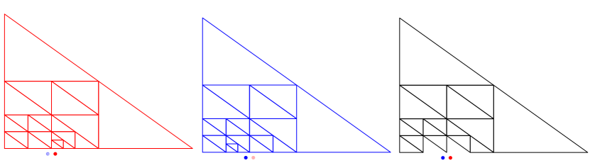
Figure 2: Adaptive integration grids used for the red target (left), blue target (center). The black grid (right) is the common set of triangles in both of the grids for which the function values of $\bm{X}^{j},K_{nm}$, and $J^{j}$ are reutilized.

Remark 9.

Adaptive integration often results in much greater accuracy than requested. With this in mind, we set $\varepsilon$ in the termination criterion to be somewhat larger than the precision requested. Our choice is based on extensive numerical experimentation and the full set of parameters used in our implementation is available at https://gitlab.com/fastalgorithms/fmm3dbie.

Remark 10.

To further improve the performance of computing $I^{j}_{nm}(\bm{x})$, we make use of two parameters: $\eta$ and $\eta_{1}<\eta$. We only use adaptive integration for the nearest targets, inside $N_{\eta_{1}}(\Gamma_{j})$. For targets $\bm{x}\in N_{\eta}(\Gamma_{j})\setminus N_{\eta_{1}}(\Gamma_{j})$, we use a single oversampled quadrature without any adaptivity. This is slightly more expensive in terms of function evaluations, but eliminates the branching queries of adaptive quadrature and allows the use of highly optimized linear algebra libraries. From extensive numerical experiments, we have found that $\eta_{1}=1.25$ provides a significant speedup.

4.4 Error Analysis

There are two sources of error in the computation of $\mathcal{S}_{k}[\sigma]$: the discretization error due to discretizing the charts $\bm{X}^{j}$ using order $p$ Vioreanu-Rokhlin nodes, and the quadrature error due to using different quadrature rules for evaluating integrals over the discretized patches. As shown in [3], the discretization error can be bounded by

$$\left|\mathcal{S}_{k}[\sigma](\bm{x})-\sum_{j=1}^{N_{\textrm{patches}}}\int_{u=0}^{1}\int_{v=0}^{1-u}G_{k}(\bm{x},\bm{X}^{j}(u,v))\sigma(u,v)J^{j}(u,v)\,du\,dv\right|\\ =\left|\mathcal{S}_{k}[\sigma](\bm{x})-\sum_{j=1}^{N_{\textrm{patches}}}L_{j}(\bm{x})\right|\leq Ch^{p},$$ (4.26)

where $h=\max_{j}R_{j}$, and some domain dependent constant $C$. For a given $\bm{x}\in\Gamma_{m}$, our method approximates the layer potential as

$$I(\bm{x})=\sum_{\ell=1}^{N(\bm{x})}G_{k}(\bm{x},\bm{X}^{m}(u_{\bm{x},\ell},v_{\bm{x},\ell}))\,\sigma(u_{\bm{x},\ell},v_{\bm{x},\ell})\,J^{m}(u_{\bm{x},\ell},v_{\bm{x},\ell})w_{\bm{x},\ell}\ +\\ \sum_{\Gamma_{j}\in N_{\eta}(\bm{x})}\sum_{\ell=1}^{n_{p}}a_{\ell}^{j}(\bm{x})\sigma^{j}_{\ell}\ +\sum_{\Gamma_{j}\in F_{\eta}(\bm{x})}\sum_{\ell=1}^{n_{q_{j}}}G_{k}(\bm{x},\bm{X}^{j}(u_{\ell,q_{j}},v_{\ell,q_{j}}))J^{j}(u_{\ell,q_{j}},v_{\ell,q_{j}})w_{\ell,q_{j}}\tilde{\sigma}^{j}_{\ell}\,,$$ (4.27)

which are approximations to $\mathcal{S}_{\textrm{Self}}$, $\mathcal{S}_{\textrm{Near}}$, and $\mathcal{S}_{\textrm{Far}}$ respectively. Here $(u_{\bm{x},\ell},v_{\bm{x},\ell}),w_{\bm{x},\ell}$ are the auxiliary nodes on the self patch, $a^{j}_{\ell}(\bm{x})$ are the near quadrature corrections computed via adpative integration, $\tilde{\sigma}^{j}_{\ell}$ is the oversampled density, and $(u_{\ell,q},v_{\ell,q}),w_{\ell,q}$, $\ell=1,2,\ldots n_{q}$ are the order $q$ Vioreanu-Rokhlin nodes on $T_{0}$. Using the estimates in Equations 4.2, 4.25 and 4.20, combined with Equation 4.26, we conclude that

$$\left|\mathcal{S}_{k}[\sigma](\bm{x})-I(\bm{x})\right|\leq Ch^{p}+\varepsilon\|\sigma\|_{\mathbb{L}^{2}(\Gamma)}\,.$$ (4.28)

Remark 11.

As shown in [3], the discretization error for evaluating $\mathcal{D}_{k}[\sigma]$ is $O(h^{p-1})$. The quadrature error analysis remains the same and we can evaluate $\mathcal{D}_{k}[\sigma](\bm{x})$ with accuracy $O(h^{p-1})+\varepsilon\|\sigma\|_{\mathbb{L}^{2}(\Gamma)}$.

5 Coupling quadratures to FMMs

For a complete description of three-dimensional FMMs applied to sums of the form (1.1), we refer the reader to the original papers [27, 2, 28, 29]. In order to understand the modifications needed for evaluating layer potentials, however, we will need to make reference to the adaptive oct-tree data structures on which the FMM is built. We briefly summarize that construction here.

5.1 Level-restricted, adaptive oct-trees

Suppose for the moment that we are given a collection of $N$ points, contained in a cube $C$. We will superimpose on $C$ a hierarchy of refinements as follows: the root of the tree is $C$ itself and defined as level 0. Level $l+1$ is obtained from level $l$ recursively by subdividing each cube at level $l$ into eight equal parts, so long as the number of points in that cube at level $l$ is greater than some specified parameter $s$. The eight cubes created in the above step are referred to as its children. Conversely, the box which was divided is referred to as their parent. When the refinement has terminated, $C$ is covered by disjoint childless boxes at various levels of the hierarchy (depending on the local density of the given points). These childless boxes are referred to as leaf nodes. For any box $D$ in the hierarchy, other boxes at the same level that touch $D$ are called its colleagues. For simplicity, we assume that the oct-tree satisfies a standard restriction - namely, that two leaf nodes which share a boundary point must be no more than one refinement level apart. In creating the adaptive data structure as described above, it is very likely that the level-restriction criterion is not met. Fortunately, assuming that the tree constructed to this point has $O(N)$ leaf nodes and that its depth is of the order $O(\log N)$, it is straightforward to enforce the level-restriction in a second step requiring $O(N\log N)$ effort with only a modest amount of additional refinement [30].

5.2 Precomputation

To reiterate, on input, we assume we are given a surface $\Gamma$ consisting of (curvilinear) triangles $\Gamma_{j}$,

$$\Gamma=\cup_{j=1}^{N_{\textrm{patches}}}\,\Gamma_{j},$$ (5.1)

each given to the desired order of accuracy $p$. Each $\Gamma_{j}$ is then discretized using $n_{p}$ points which are the images under the map $\bm{X}^{j}:T_{0}\to\mathbb{R}^{3}$ of the Vioreanu-Rokhlin nodes on the standard simplex $T_{0}$. We will refer to these as the discretization nodes, on which we assume that samples of the density $\sigma$ are known. The total number of such points is $N=N_{\textrm{patches}}\times n_{p}$. As above, we let $\bm{c}_{j}$ denote the centroid of the $j$th patch and $R_{j}$ the radius of the smallest sphere centered at $\bm{c}_{j}$ that contains $\Gamma_{j}$. We assume there are $N_{T}$ targets, which could be either the discretization nodes themselves, a collection of off-surface points, or both.

In coupling the FMM to local quadratures, we need to determine, for each surface patch, which targets are in its near field and what order Vioreanu-Rokhlin quadratures are needed for the far field computation. Both are controlled by the parameter $\eta$, as discussed in Section 4.1. The default value for $\eta$ is $2.75$, $2$, or $1.25$ depending on whether the desired order of accuracy is $p\leq 4$, $4<p\leq 8$ or $p>8$, respectively. The first step is to build an adaptive oct-tree based on the patch centroids $\{\bm{c}_{j}\}$ and the target locations, with one minor modification. That modification is to prevent triangle centroids associated with large triangles from propagating to fine levels during the tree construction. For this, suppose $\bm{c}_{j}$ is in some box, denoted $D(\bm{c}_{j})$ at level $l$, and let $d$ denote the linear dimension of $D(\bm{c}_{j})$. If $2\eta\,R_{j}>d$, then we leave the centroid associated with $D(\bm{c}_{j})$, while allowing smaller triangles and/or targets to be associated with the children. We will say that $\Gamma_{j}$ is tethered at level $l$.

The near field for each patch is now easy to determine. For each triangle $\Gamma_{j}$, let $D(\bm{c}_{j})$ denote the box to which the triangle centroid is associated - either a leaf node or the box at a coarser level $l$ if is tethered there. Clearly, if $D(\bm{c}_{j})$ is not a leaf box, then the near field region $B_{\eta R_{j}}(\bm{c}_{j})$ is contained within $D(\bm{c}_{j})$ and its colleagues. If $D(\bm{c}_{j})$ is a leaf box, then the near field region $B_{\eta R_{j}}(\bm{c}_{j})$ is contained within the union of $D(\bm{c}_{j})$, its colleagues, and leaf boxes which are larger in size than $D(\bm{c}_{j})$ and which share a boundary with $D(\bm{c}_{j})$. Scanning those colleagues, all targets $\bm{x}$ that do not lie on $\Gamma_{j}$ itself and satisfy the criterion

$$|\bm{x}-\bm{c}_{j}|<\eta R_{j}$$

are assigned to the near field list for $\Gamma_{j}$. One can then compute the near field quadratures using the method of Section 4.3 for each point in the target list. This requires storing a matrix of dimension $N_{near}(j)\times n_{p}$, where $N_{near}(j)$ is the size of the target list. We will denote this matrix by ${\cal N}_{j}$.

Assuming one wishes to evaluate the layer potential on surface, we also need to compute the self interactions for each triangle using the generalized Gaussian quadrature scheme of [8, 9], as described in Section 4. This requires storing an $n_{p}\times n_{p}$ matrix for each patch, which we will denote by ${\cal S}_{j}$.

Once the near field work has been carried out, the far field quadrature order $q_{j}$ is determined, as described in Section 4.2. One can then interpolate from the $n_{p}$ discretization nodes on $\Gamma_{j}$ to the $n_{q_{j}}$ quadrature nodes on $\Gamma_{j}$ using the Koornwinder basis for interpolation. We will denote by $N_{over}$ the total number of oversampled points used: $N_{over}=\sum_{i=1}^{N_{\textrm{patches}}}n_{q_{i}}$.

5.3 Fast evaluation of layer potentials

The simplest FMM-based scheme for evaluating a layer potential is to call the point-based FMM in the form (1.1), with $N_{over}$ sources and $N_{T}$ targets. For every target, if it is in the near field of patch $\Gamma_{j}$, one subtracts the contribution made in the naive, point-based FMM calculation from the $n_{q}$ oversampled points on that patch. The potential at the target can then be incremented by the appropriate, near field quadrature-corrected interactions, using the stored matrix ${\cal N}_{j}$. If the target is on surface (one of the discretization nodes on $\Gamma_{j}$ itself), the correct self interaction is obtained from the precomputed matrix ${\cal S}_{j}$.

We refer to the algorithm above as the subtract-and-add method. It has the drawback that it could suffer from catastrophic cancellation for dense discretizations with highly adaptive oct-trees since the near field point contributions within the naive FMM call are spurious and could be much greater in magnitude than the correct contributions. (In practice, we have not detected any such loss of accuracy, at least for single or double layer potentials.)

For readers familiar with the FMM, it is clear that one could avoid the need to compute and then subtract spurious contributions, by disabling the direct (near neighbor) interaction step in the FMM. When looping over the leaf nodes, for each source-target pair, one can first determine whether the source is on a patch for which the target is in the far field. If it is, carry out the direct interaction. If it is in the near field, omit the direct interaction. When the FMM step is completed, the subsequent processing takes place as before, but there is no need to subtract any spurious contributions.

It is, perhaps, surprising that the subtract-and-add method is faster in our current implementation, even though more flops are executed. This is largely because of the logical overhead and the bottlenecks introduced in loop unrolling and other compiler-level code optimizations.

Remark 12.

The adaptive oct-tree used in the point FMM is different from the one used for determining the near field of the patches. The latter is constructed based on centroid and target locations, while the point FMM oct-tree is constructed based on oversampled source and target locations. Thus, different termination criteria can be chosen for the construction of these oct-trees in order to optimize the performance of the separate tasks.

Since the additional processing required for evaluating layer potentials is decoupled from the algorithm used for accelerating the far field interactions, one could use any fast hierarchical algorithm like the FMM, an FFT-based scheme like fast Ewald summation, or a multigrid-type PDE solver.

6 Numerical examples

In this section, we illustrate the performance of our approach. For Examples 6.1, 6.2, and 6.3, we consider a twisted torus as the geometry (typical of stellarator design in plasma physics applications). The boundary $\Gamma$ is parameterized by $\bm{X}:[0,2\pi]^{2}\to\Gamma$ with

$$\bm{X}(u,v)=\sum_{i=-1}^{2}\sum_{j=-1}^{1}\delta_{i,j}\begin{bmatrix}\cos{v}\cos{((1-i)\,u+j\,v)}\\ \sin{v}\cos{((1-i)\,u+j\,v)}\\ \sin{((1-i)\,u+j\,v)}\end{bmatrix}\,,$$ (6.1)

where the non-zero coefficients are $\delta_{-1,-1}=0.17$, $\delta_{-1,0}=0.11$, $\delta_{0,0}=1$, $\delta_{1,0}=4.5$, $\delta_{2,0}=-0.25$, $\delta_{0,1}=0.07$, and $\delta_{2,1}=-0.45$. (See Fig. 3.)

The code was implemented in Fortran and compiled using the GNU Fortran 10.2.0 compiler. We use the point-based FMMs from the FMM3D package (https://github.com/flatironinstitute/FMM3D). All CPU timings in these examples were obtained on a laptop using a single core of an Intel i5 2.3 GHz processor.

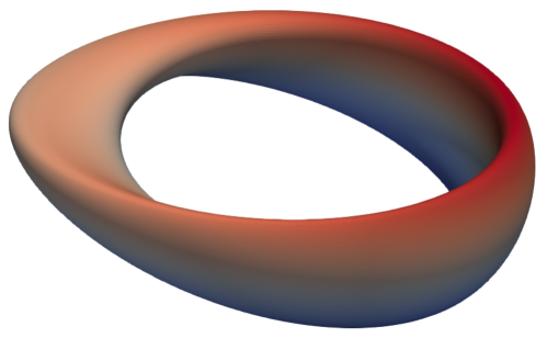
Figure 3: The boundary of a stellarator like geometry. The surface is colored using its z-coordinate

We use the following metrics to demonstrate the performance of our approach. As above, for discretization order $p$, we let $n_{p}=p(p+1)/2$, and we let $q_{j}$ denote the far-field quadrature order for $\Gamma_{j}$. The user-specified precision is denoted by $\varepsilon$. Recall that the total number of discretization points on the boundary is denoted by $N=N_{\textrm{patches}}\cdot n_{p}$ and that the total number of oversampled nodes is denoted by $N_{\textnormal{over}}=\sum_{j=1}^{N_{\textrm{patches}}}n_{q_{j}}$. We define the oversampling parameter by $\alpha=N_{\textnormal{over}}/N$. The memory requirements per discretization node for storing all interactions in $\mathcal{S}_{\textrm{Near}}$ are given by

$$m=\frac{n_{p}\left(\sum_{j=1}^{N_{\textrm{patches}}}N_{near}(j)+n_{p}\right)}{N}.$$ (6.2)

This accounts for both off-surface targets and on surface evaluation.

Let $T_{\textnormal{init}}$ denote the time required to precompute all near field quadrature corrections and let $T_{\textnormal{LP}}$ denote the time for evaluating the layer potential given the precomputed near field quadratures Then, the quantities $S_{\textnormal{init}}=N/T_{\textnormal{init}}$, and $S_{\textnormal{LP}}=N/T_{\textnormal{LP}}$, are the speeds of the corresponding steps, measured in points processed per second.

One feature of the surface triangulation that has some influence on speed is the aspect ratio of the patches. Letting $\sigma_{1},\sigma_{2}$ be the eigenvalues of the first fundamental form of $\Gamma_{j}$, we define its aspect ratio by

$$a_{j}=\sqrt{\frac{\int_{\Gamma_{j}}\left(\frac{\sigma_{1}}{\sigma_{2}}\right)^{2}da(\bm{y})}{\int_{\Gamma_{j}}da(\bm{y})}}\,.$$ (6.3)

We let $a_{\textnormal{max}}=\max_{j}a_{j}$ and $a_{\textnormal{avg}}=\sum_{j}a_{j}/N_{\textrm{patches}}$, the maximum aspect ratio and the average aspect ratio over all triangles, respectively.

6.1 Memory and oversampling requirements

To illustrate the performance of our method as a function of the order of accuracy $p$ and the requested precision $\varepsilon$, we consider the evaluation of the single layer potential $\mathcal{S}[\sigma]$ with frequency $k=1$ on the stellarator geometry discretized with $N_{\textrm{patches}}=2400$ (the diameter of the stellarator with $k=1$ is approximately 1.7 wavelengths). In LABEL:tab:numerical-perf-res, we tabulate the memory requirements per point $m$, the oversampling $\alpha$, and the speeds $S_{\textnormal{init}}$ and $S_{\textnormal{LP}}$, as we vary $p$ and $\varepsilon$. The scheme behaves as expected: for fixed $p$, as $\varepsilon\rightarrow 0$, $\alpha$ increases while $S_{\textnormal{init}}$ and $S_{\textnormal{LP}}$ decrease. The oversampling parameter $\alpha$ depends on both $p$ and $\varepsilon$, as discussed in Section 4.2.

6.2 Effect of aspect ratio

To investigate the effect of triangle quality on the performance of our method, we vary the average aspect ratio of the discretization. The task at hand is again to compute $\mathcal{S}[\sigma]$ with $k=1$ on the stellarator, while varying the triangulation without a significant change in the total number of patches. In LABEL:tab:numerical-asp-res, we tabulate $a_{\textnormal{avg}}$, $N_{\textrm{patches}}$, $\alpha$, $m$, $S_{\textnormal{init}}$, and $S_{\textnormal{LP}}$ for $p=4$ and $\varepsilon=5\cdot 10^{-7}$. We note that (except for the oversampling parameter), the performance of the approach deteriorates as the average aspect ratio of the discretization is increased, especially in the precomputation phase.

6.3 Order of convergence

To demonstrate the accuracy of our approach, we consider two tests. First, we verify Green’s identity along the surface:

$$\frac{u}{2}=\mathcal{S}_{k}\left[\frac{\partial u}{\partial n}\right]-\mathcal{D}_{k}[u]\,,$$ (6.4)

where $u$ is the solution to the Helmholtz equation in the interior of the domain $\Omega$ generated by a point source located in the exterior. The second test is to use the combined field representation (3.2) to solve the Dirichlet problem for an unknown density $\sigma$. With the right-hand side in the corresponding integral equation (3.5) taken to be a known solution $u$, $\sigma$ satisfies

$$\frac{\sigma}{2}+\mathcal{D}_{k}[\sigma]-ik\mathcal{S}_{k}[\sigma]=u,\qquad\text{on }\Gamma.$$ (6.5)

We can then check that $u$ is correctly reproduced at any point in the exterior. For both of these tests, we discretize the stellarator using $N_{\textrm{patches}}=600$, $2400$, and $9600$, and compute the layer potentials with a tolerance of $\varepsilon=5\times 10^{-7}$ for both the quadratures and the FMM.

In LABEL:fig:ooc, we plot the relative $L^{2}$ error in Green’s identity $\varepsilon_{g}$ (left), and the relative $L^{\infty}$ error at a point in the interior $\varepsilon_{a}$ (right) as we vary the order of discretization. Note that in both tests, the errors decrease at the rate $h^{p-1}$ until the tolerance $\varepsilon$ is reached. This is consistent with the analysis in [3].

6.4 Large-scale examples

We demonstrate the performance of our solver on several large-scale problems. We first solve for the electrostatic field induced by an interdigitated capacitor, followed by Dirichlet and Neumann boundary value problems governed by the Helmholtz equation in the exterior of an aircraft. Our last example involves scattering in a medium with multiple sound speeds, modeled after a Fresnel lens. The results in this section were obtained using an Intel Xeon Gold 6128 Desktop with 24 cores.

Interdigitated capacitor

A challenging problem in electrostatics is the calculation of the capacitance of a configuration of two perfect compact conductors with complicated contours, which may also be close to touching. (See Figure 4.) The capacitance is defined as the ratio $C=Q/V$, where $V$ is the potential difference between the conductors, $Q$ is the total charge held on one conductor and $-Q$ is the total charge held on the other. In simulations, $C$ can be computed in two ways. First, one can solve the Dirichlet problem for the electrostatic potential $u$, with $u=0$ on one conductor and $u=1$ on the other. From the computed solution, the total charge can be obtained via the integral [31]

$$Q=\int_{\Gamma}\frac{\partial u}{\partial n}(\bm{x}^{\prime})\,da(\bm{x}^{\prime}).$$ (6.6)

The capacitance is then $C=Q/1=Q$.

A second (equivalent) approach, which we will take here, is to place a net charge $q_{1}=-1$ on one conductor $\Omega_{1}$ with boundary $\Gamma_{1}$ and a net charge of $q_{2}=1$ on the other conductor $\Omega_{2}$ with boundary $\Gamma_{2}$. One can then determine the corresponding potential difference by solving the following boundary value problem for the potential $u$ in the domain $E$ exterior to $\Omega_{1}$ and $\Omega_{2}$, i.e. the domain $E=\mathbb{R}^{3}\setminus(\Omega_{1}\cup\Omega_{2})$:

$$\Delta u =0, \bm{x}\in E,$$ (6.7)

$$u =V_{i}, \bm{x}\text{ on }\Gamma_{i},,$$

$$-\int_{\Gamma_{j}}\frac{\partial u}{\partial n}\,da =q_{i},$$

$$u \to 0 \text{ as }|\bm{x}|\to\infty.$$

Here, the constants $V_{1}$, $V_{2}$ are unknowns as well as the potential $u$. The elastance of the system is then given by $P=(V_{2}-V_{1})/(q_{2}-q_{1})=(V_{2}-V_{1})/2$. It is the inverse of the corresponding capacitance $C=1/P=2/(V_{2}-V_{1})$. This formulation (which can involve more than two conductors) is generally referred to as the elastance problem (see [32] and the references therein). PDEs of this type where Dirichlet data is specified up to an unknown constant are sometimes called modified Dirichlet problems [33].

We represent the solution $u$ using the combined field representation,

$$u=S_{0}[\rho]+D_{0}[\rho],$$ (6.8)

where $\rho$ is an unknown density. Imposing the boundary conditions on $\Gamma_{i}$, $\rho$ must satisfy the integral equation

$$\rho/2+D_{0}[\rho]+S_{0}[\rho] =V_{i}, \bm{x}\text{ on }\Gamma_{i},$$ (6.9)

$$\int_{\Gamma_{i}}\rho =-q_{i}, i=1,2.$$

We discretize the surface $\Gamma$ with $N_{\textrm{patches}}=29,888$ and $p=4$, and then solve the resulting linear system of size $N=298,882$ using GMRES. We set the quadrature tolerance $\varepsilon=5\times 10^{-7}$. For this setup, $T_{\textnormal{init}}=6.7$s, $\alpha=2.98$, $m=154.2$. GMRES converged to a relative residual of $5\times 10^{-7}$ in 25 iterations, and the solution was obtained in $128.4$s. The reference capacitance for the system was computed by refining each patch until it had converged to 5 significant digits, given by $2237.1$. The relative error in the computed capacitance was $2.2\times 10^{-4}$. In Figure 4, we plot the computational mesh and the solution $\rho$ on the surface of the conductors.

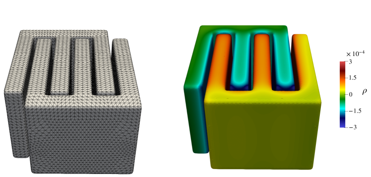
Figure 4: (left) A 4th-order computational mesh of the boundary, and (right) the solution $\rho$ to Equation 6.9

Scattering from an airplane (sound-soft)

In this section we demonstrate the performance of our method on a moderate frequency acoustic scattering problem. The model airplane is $49.3$ wavelengths long, with a wingspan of $49.2$ wavelengths and a vertical height of $13.7$ wavelengths, which we assume has a sound-soft boundary, satisfying Dirichlet boundary conditions (see section 3). The plane also has several multiscale features: 2 antennae on the top of the fuselage, and 1 control unit on the bottom of the fuselage. (See Figure 6.) The plane is discretized with $N_{\textrm{patches}}=125,344$, and $p=4$ resulting in $N=1,253,440$ discretization points. The ratio of the largest to the smallest patch size, measured by the enclosing sphere radius $R_{j}$ in Equation 4.6, is $483.9$. In Figure 5, we plot a histogram of the patch sizes $R_{j}$, and the aspect ratios of the patches on the plane. The worst case patch has an aspect ratio of $35$, but only $322$ patches out of the total $125,344$ have an aspect ratio of greater than $10$.

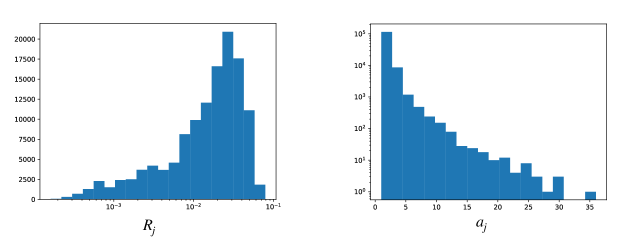
Figure 5: Histogram of size of patches $R_{j}$ (left), and aspect ratio $a_{j}$ right.

In order to have an analytic reference solution, we assume the Dirichlet boundary data $u|_{\Gamma}$ for the governing exterior Helmholtz equation is generated using a collection of $123$ interior sources, $19$ of which are in the tail. Using a combined field representation

$$u=\mathcal{D}_{k}[\sigma]-ik\,\mathcal{S}_{k}[\sigma],$$

imposing the Dirichlet condition yields the combined field integral equation for the unknown density $\sigma$:

$$\frac{\sigma}{2}+\mathcal{D}_{k}[\sigma]-ik\mathcal{S}_{k}[\sigma]=u|_{\Gamma}\,.$$ (6.10)

For a quadrature tolerance of $5\times 10^{-7}$, $T_{\textnormal{init}}=75.86$s, the oversampling factor $\alpha=4.51$, and the memory cost per discretization point is $m=149.6$. GMRES converged to a relative residual of $5\times 10^{-7}$ in $59$ iterations, and the solution was obtained in $4,694$s. We plot the solution on a $301\times 301$ lattice of targets on a slice which cuts through the wing edge, whose normal is given by $(0,0,1)$. For targets in the interior of the airplane, we set the error to $1\times 10^{-6}$ since the computed solution there is not meaningful. The layer potential evaluation at all targets required only $T_{\textnormal{init}}+T_{\textnormal{quad}}=104.37$s. In Figure 6, we plot the density $\sigma$ on the airplane surface and the relative error on the slice with $301\times 301$ targets. The maximum relative error at all targets is $5\times 10^{-4}$.

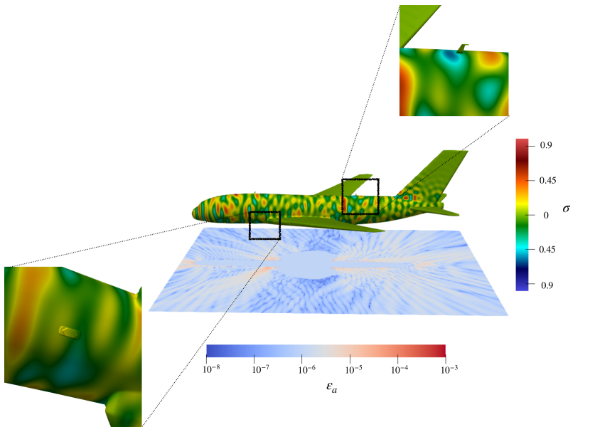
Figure 6: The solution $\sigma$ to Equation 6.10, and the relative error in the solution at a grid of $301\times 301$ targets on a horizontal slice intersecting the wing edge. Zoomed in views of one antenna (top right) and the control unit (bottom left) indicate the extent of the fine multiscale features.

Scattering from an airplane (sound-hard)

In this section we solve the Helmholtz equation in the exterior of the plane, assuming Neumann boundary conditions instead. These arise in the modeling of sound-hard scatterers [26]. We will use the following regularized combined field integral representation of [34] for the solution:

$$u=\mathcal{S}_{k}[\sigma]+i\alpha\mathcal{D}_{k}\left[\mathcal{S}_{i|k|}[\sigma]\right].$$ (6.11)

Applying the boundary condition $\partial u/\partial n=g$ along $\Gamma$ leads to the second-kind integral equation:

$$-\frac{\sigma}{2}+\mathcal{S}^{\prime}_{k}[\sigma]+i\alpha\mathcal{D}^{\prime}_{k}\left[\mathcal{S}_{i|k|}[\sigma]\right]=g.$$ (6.12)

Using a well-known Calderón identity for the operator $\mathcal{D}^{\prime}_{i|k|}\mathcal{S}_{i|k|}$ [35], this equation can be re-written so as to avoid the application of the hypersingular operator $\mathcal{D}_{k}^{\prime}$:

$$-\left(\frac{2+i\alpha}{4}\right)\sigma+\mathcal{S}^{\prime}_{k}[\sigma]+i\alpha\left(\mathcal{D}^{\prime}_{k}-\mathcal{D}^{\prime}_{i|k|}\right)\left[\mathcal{S}_{i|k|}[\sigma]\right]+i\alpha\mathcal{S}^{\prime 2}_{i|k|}[\sigma]=g.$$ (6.13)

A number of different possibilities for the regularizing operator are available depending on the frequency range (see [36, 37]). Examining the above integral equation, it is clear that a total of four separate FMM calls and four local quadrature corrections will be needed.

In order to have an analytic reference solution, we generate the Neumann boundary data $u|_{\Gamma}$ for the governing exterior Helmholtz equation by using the same $123$ interior sources as in the Dirichlet problem. For a quadrature tolerance of $5\times 10^{-7}$, $T_{\textnormal{init}}=387.4$s, the oversampling factor $\alpha=4.51$, and the memory cost per discretization point is $m=598.3$. GMRES converged to a relative residual of $5\times 10^{-7}$ in $35$ iterations, and the solution was obtained in $7617$s. We plot the solution on the $301\times 301$ lattice of targets used for the Dirichlet problem. As before, for targets in the interior of the airplane, we set the error to $1\times 10^{-6}$ since the computed solution there is not meaningful. The layer potential evaluation at all targets required only $T_{\textnormal{init}}+T_{\textnormal{quad}}=159.6$s. In Figure 7, we plot the induced density $\sigma$ on the airplane surface and the relative error on the slice with $301\times 301$ targets. The maximum relative error at all targets is $5\times 10^{-4}$.

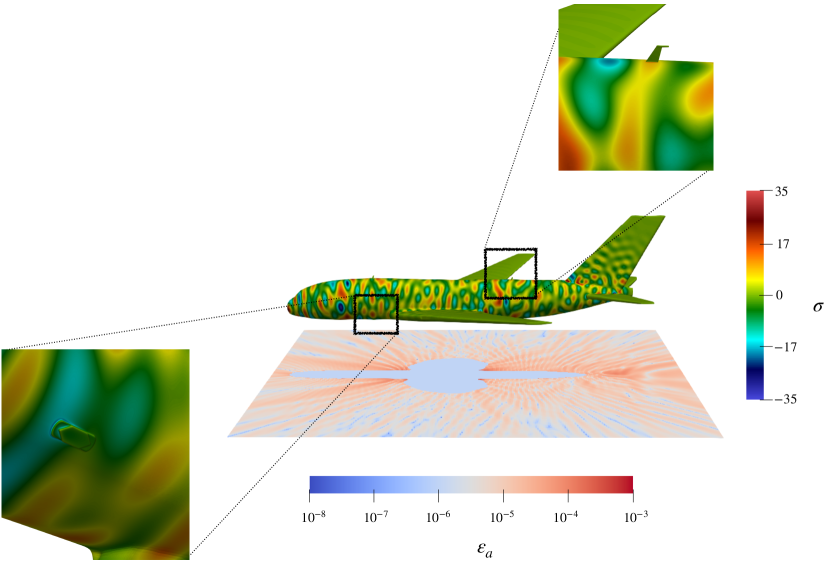
Figure 7: The solution $\sigma$ to integral equation (6.13), and the relative error in the solution to the PDE at a grid of $301\times 301$ targets on a horizontal slice intersecting the wing edge. Zoomed in views of one antenna (top right) and the control unit (bottom left) indicate the extent of the fine multiscale features.

Scattering through a Fresnel lens (multiple sound speeds)

In this section we solve the Helmholtz transmission problem, i.e. scattering through media with various sound speeds, in a Fresnel lens geometry (see Figure 8). The Helmholtz parameter for the interior region (the lens) is $k=\omega\sqrt{\epsilon\mu}$ and for the exterior region (free space) is $k_{0}=\omega\sqrt{\epsilon_{0}\mu_{0}}$. We assume that the known incoming field $u^{\operatorname{inc}}$ exists only in the exterior, so that the total field in the exterior is given by $u_{t}=u_{0}+u^{\operatorname{inc}}$ where $u_{0}$ is the scattered field. In the interior, the total field is merely $u_{t}=u$, with $u$ the scattered field.

In the piecewise constant sound speed setup, we enforce the following transmission conditions across interfaces:

$$u_{0}-u =-u^{\operatorname{inc}}|_{\Gamma},$$ (6.14)

$$\frac{1}{\epsilon_{0}}\frac{\partial u_{0}}{\partial n}-\frac{1}{\epsilon_{1}}\frac{\partial u}{\partial n} =-\frac{1}{\epsilon_{0}}\frac{\partial u^{\operatorname{inc}}}{\partial n}\Big{|}_{\Gamma}.$$

The scattered field in the exterior region, $u_{0}$, and in the interior region, $u$, are represented as, respectively [26]:

$$u_{0} =\epsilon_{0}\mathcal{D}_{k_{0}}[\rho]+\epsilon_{0}^{2}\mathcal{S}_{k_{0}}[\sigma],$$ (6.15)

$$u =\epsilon\mathcal{D}_{k}[\rho]+\epsilon^{2}\mathcal{S}_{k}[\sigma].$$

This leads to the system of boundary integral equations along $\Gamma$

$$\Big{(}\frac{\epsilon_{0}+\epsilon}{2}\Big{)}\rho+\Big{(}\epsilon_{0}\mathcal{D}_{k_{0}}-\epsilon\mathcal{D}_{k}\Big{)}[\rho]+\Big{(}\epsilon_{0}^{2}\mathcal{S}_{k_{0}}-\epsilon^{2}\mathcal{S}_{k}\Big{)}[\sigma] =-u^{\operatorname{inc}},$$ (6.16)

$$\Big{(}\frac{\epsilon_{0}+\epsilon}{2}\Big{)}\sigma-\Big{(}\mathcal{D}^{\prime}_{k_{0}}-\mathcal{D}^{\prime}_{k}\Big{)}[\rho]-\Big{(}\epsilon_{0}\mathcal{S}^{\prime}_{k_{0}}-\epsilon\mathcal{S}^{\prime}_{k}\Big{)}[\sigma] =-\frac{1}{\epsilon_{0}}\frac{\partial u^{\operatorname{inc}}}{\partial n}.$$

In the following example, the Fresnel lens has $\epsilon=2$, $\mu=1$ and as usual, in free-space $\epsilon_{0}=\mu_{0}=1$. The angular frequency is set to be $\omega=1+\sqrt{2}$, and the annular step size in the lens equals 1. Relative to the exterior wavenumber, the Fresnel lens is 19.11 wavelengths in diameter and has a height of 0.84 wavelengths. The geometry was designed in GiD [38], and a 4th-order curvilinear mesh was constructed using the method described in [39]. The mesh consists of 62,792 curvilinear triangles, each discretized to 5th order yielding a total of 941,880 discretization points. See Figure 8.

We solve the transmission problem in response to an incoming plane wave $u^{inc}=e^{ik_{0}z}$. For a quadrature tolerance of $5\times 10^{-7}$, $T_{\textnormal{init}}=238.2$s, the oversampling factor $\alpha=3.07$, and the memory cost per discretization point is $m=762.0$. GMRES converged to a relative residual of $5\times 10^{-7}$ in $294$ iterations, and the solution was obtained in $23029$s. In Figure 8 we plot the absolute value of the total field $|u_{t}|=|u_{0}+u^{inc}|$ on a $1000\times 1000$ lattice of targets in the $yz$ plane in the exterior region. The layer potential evaluation at all targets required only $T_{\textnormal{init}}+T_{\textnormal{quad}}=81.1$s. We also plot the real part of the density $\rho$ on the surface of the lens.

The accuracy of the solution is estimated by solving a transmission problem whose boundary data is computed using known solutions to the Helmholtz equation in the interior and exterior (the interior Helmholtz solution is the potential due to a point source in the exterior and the exterior Helmholtz solution is the potential due to a point source in the interior). The maximum relative error for the computed solution at the same target grid as above is $8.4\times 10^{-5}$.

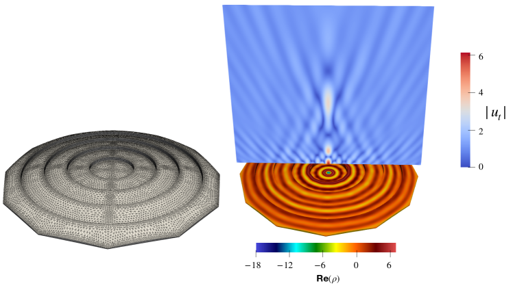
Figure 8: On the left, we illustrate the triangulation of the lens surface. On the right is a plot of the real part of the solution $\rho$ to Equation 6.16 on the surface of the lens and the absolute value of the total field above the lens where the central focusing of the beam is clearly visible.

7 Conclusions

In this paper, we have presented a robust, high-order accurate method for the evaluation of layer potentials on surfaces in three dimensions. While our examples have focused on the Laplace and Helmholtz equations, the underlying methodology extends naturally to other problems in mathematical physics where the governing Green’s function is singular – thereby requiring specialized quadrature schemes – but compatible with fast multipole acceleration in the far field.

To determine the highest performance scheme, we implemented generalized Gaussian quadrature [8, 9, 10, 11], QBX [21, 16, 17, 18], and coordinate transformation schemes similar to [12, 14, 19]. After various code optimizations (at least for surfaces defined as collections of curved, triangular patches), we found that generalized Gaussian quadrature with careful reuse of precomputed, hierarchical, adaptive interpolation tables was most efficient, as illustrated in the preceding section. It may be that an even better local quadrature scheme emerges in the future (in particular, extensions of the idea presented in [40] look quite promising). In that case, as discussed in Section 5, coupling to the FMM will be fundamentally unchanged.

A useful feature of locally corrected quadrature rules (of any kind) is that the procedure is trivial to parallelize by assigning a different patch to each computational thread. Thus, acceleration on multi-core or high performance platforms is straightforward.

Finally, although we limited ourselves here to evaluating layer potentials and solving integral equations iteratively, we note that our quadrature generation scheme and oct-tree data structure are compatible for use with fast direct solvers [10, 41, 42, 43, 44, 45, 46, 47, 48]. These require access to small blocks of the system matrix in an effort to find a compressed representation of the inverse.

There are still a number of open questions that remain to be addressed, including the development of rules for surfaces with edges and corners and the coupling of layer potential codes with volume integral codes to solve inhomogeneous or variable-coefficient partial differential equations using integral equation methods. These are all ongoing areas of research.

References

- [1] L. Greengard, J. Huang, V. Rokhlin, S. Wandzura, Accelerating Fast Multipole Methods for the Helmholtz Equation at Low Frequencies, IEEE Comput. Sci. Eng. 5 (3) (1998) 32–38.
-
[2]
H. Cheng, W. Y. Crutchfield, Z. Gimbutas, L. Greengard, J. F. Ethridge,
J. Huang, V. Rokhlin, N. Yarvin, J. Zhao,
A wideband fast multipole
method for the Helmholtz equation in three dimensions, J. Comput. Phys.
216 (2006) 300–325.
URL http://dx.doi.org/10.1016/j.jcp.2005.12.001 - [3] K. E. Atkinson, D. Chien, Piecewise polynomial collocation for boundary integral equations, SIAM J. Scientific Computing 16 (1995) 651–681.
- [4] K. E. Atkinson, The Numerical Solution of Integral Equations of the Second Kind, Cambridge University Press, New York, NY, 1997.
- [5] A. M. J, M. J. Berger, M. J. E, Robust and efficient Cartesian mesh generation for component-based geometry, AIAA J. 36 (1998) 952–960.
- [6] J. Bell, M. Berger, J. Saltzman, M. Welcome, Three-dimensional adaptive mesh refinement for hyperbolic conservation laws, SIAM J. Scientific Computing 15 (1994) 127–138.
- [7] H. Johanssen, P. Colella, A Cartesian grid embedded boundary method for Poisson’s equation on irregular domains, J. Comput. Phys. 147 (2) (1998) 60–85.
- [8] J. Bremer, Z. Gimbutas, A Nyström method for weakly singular integral operators on surfaces, J. Comput. Phys. 231 (2012) 4885–4903.
- [9] J. Bremer, Z. Gimbutas, On the numerical evaluation of singular integrals of scattering theory, J. Comput. Phys. 251 (2013) 327–343.
-
[10]
J. Bremer, A. Gillman, P.-G. Martinsson,
A high-order accelerated
direct solver for integral equations on curved surfaces, BIT Num. Math. 55
(2015) 367–397.
URL http://doi.org/10.1007/s10543-014-0508-y - [11] J. Bremer, Z. Gimbutas, V. Rokhlin, A nonlinear optimization procedure for generalized Gaussian quadratures, SIAM J. Sci. Comput. 32 (4) (2010) 1761–1788.
- [12] O. P. Bruno, L. A. Kunyansky, A fast, high-order algorithm for the solution of surface scattering problems: Basic implementation, tests, and applications, J. Comput. Phys. 169 (1) (2001) 80–110.
- [13] O. Bruno, E. Garza, A Chebyshev-based rectangular-polar integral solver for scattering by geometries describedby non-overlapping patches, J. Comput. Phys. (2020) 109740doi:10.1016/j.jcp.2020.109740.
- [14] D. Malhotra, A. Cerfon, L.-M. Imbert-Gérard, M. O’Neil, Taylor states in stellarators: a fast high-order boundary integral solver, J. Comput. Phys. 397 (2019) 108791.
- [15] S. Erichsen, S. A. Sauter, Efficient automatic quadrature in 3-d Galerkin BEM, Comput. Methods Appl. Mech. Engrg. 157 (1998) 215–224.
- [16] M. Siegel, A.-K. Tornberg, A local target specific quadrature by expansion method for evaluation of layer potentials in 3d, J. Comput. Phys. 364 (2018) 365–392.
- [17] M. Wala, A. Klöckner, A fast algorithm for quadrature by expansion in three dimensions, J. Comput. Phys. 388 (2018) 655–689.
- [18] M. Wala, A. Klöckner, Optimization of fast algorithms for global quadrature by expansion using target-specific expansions, J. Comput. Phys. 403 (2020).
- [19] L. Ying, G. Biros, D. Zorin, A high-order 3D boundary integral equation solver for elliptic PDEs in smooth domains, J. Comput. Phys. 219 (1) (2006) 247–275.
- [20] M. G. Duffy, Quadrature over a pyramid or cube of integrands with a singularity at a vertex, SIAM, J. Numer. Anal. 19 (1982) 1260–1262.
- [21] A. Klöckner, A. Barnett, L. Greengard, M. O’Neil, Quadrature by Expansion: A new method for the evaluation of layer potentials, J. Comput. Phys. 252 (2013) 332–349.
- [22] T. Koornwinder, Two-variable analogues of the classical orthogonal polynomials, in: Theory and application of special functions (Proc. Advanced Sem., Math. Res. Center, Univ. Wisconsin, Madison, Wis., 1975), Academic Press New York, 1975, pp. 435–495.
- [23] L. N. Trefethen, Approximation Theory and Approximation Practice, SIAM, Philadelphia, PA, 2013.
- [24] H. Xiao, Z. Gimbutas, A numerical algorithm for the construction of efficient quadrature rules in two and higher dimensions, Computers & mathematics with applications 59 (2) (2010) 663–676.
- [25] B. Vioreanu, V. Rokhlin, Spectra of Multiplication Operators as a Numerical Tool, SIAM J. Sci. Comput. 36 (2014) A267–A288.
- [26] D. Colton, R. Kress, Integral Equation Methods in Scattering Theory, John Wiley & Sons, Inc., 1983.
- [27] H. Cheng, L. Greengard, V. Rokhlin, A fast adaptive multipole algorithm in three dimensions, J. Comput. Phys. 155 (2) (1999) 468–498.
- [28] L. Greengard, V. Rokhlin, A new version of the Fast Multipole Method for the Laplace equation in three dimensions, Acta Numerica 6 (1997) 229–269.
- [29] L. Greengard, J. Huang, A new version of the fast multipole method for screened coulomb interactions in three dimensions, J. Comput. Phys. 180 (2002) 642–658.
- [30] M. de Berg, O. Cheong, M. Kreveld, M. Overmars, Computational Geometry: Algorithms and Applications, Springer, 2008.
- [31] J. D. Jackson, Classical Electrodynamics, 3rd Edition, Wiley, New York, NY, 1999.
- [32] M. Rachh, L. Greengard, Integral equation methods for elastance and mobility problems in two dimensions, SIAM Journal on Numerical Analysis 54 (5) (2016) 2889–2909.
- [33] S. G. Mikhlin, Integral equations: and their applications to certain problems in mechanics, mathematical physics and technology, Elsevier, 2014.
- [34] O. Bruno, T. Elling, C. Turc, Regularized integral equations and fast high-order solvers for sound-hard acoustic scattering problems, Int. J. Num. Meth. Engin. 91 (2012) 1045–1072.
- [35] J.-C. Nedelec, Acoustic and Electromagnetic Equations, Springer, New York, NY, 2001.
- [36] D. Colton, R. Kress, Inverse Acoustic and Electromagnetic Scattering Theory, Springer, New York, NY, 2012.
- [37] F. Vico, L. Greengard, Z. Gimbutas, Boundary integral equation analysis on the sphere, Numer. Math. 128 (2014) 463–487.
- [38] International Center for Numerical Methods in Engineering (CIMNE), GiD: The Personal Pre- and Post-processor, gidhome.com (2020).
- [39] F. Vico, L. Greengard, M. O’Neil, M. Rachh, A fast boundary integral method for high-order multiscale mesh generation, SIAM J. Sci. Comput. 42 (2) (2020) A1380–A1401.
- [40] B. Wu, P.-G. Martinsson, Corrected Trapezoidal Rules for Boundary Integral Equations in Three Dimensions, arXiv [math.NA] 2007.02512 (2020).
- [41] L. Greengard, D. Gueyffier, P.-G. Martinsson, V. Rokhlin, Fast direct solvers for integral equations in complex three-dimensional domains, Acta Numerica 18 (2009) 243–275.
- [42] K. L. Ho, L. Greengard, A fast direct solver for structured linear systems by recursive skeletonization, SIAM J. Sci. Comput. 34 (2012) A2507–A2532.
- [43] P.-G. Martinsson, V. Rokhlin, A fast direct solver for boundary integral equations in two dimensions, J. Comput. Phys 205 (2005) 1–23.
- [44] S. Börm, Directional -matrix compression for high-frequency problems, Num. Lin. Alg. Appl. 24 (6) (2017) e2112.
- [45] H. Guo, Y. Liu, J. Hu, E. Michielssen, A Butterfly-Based Direct Integral Equation Solver Using Hierarchical LU Factorization for Analyzing Scattering from Electrically Large Conducting Objects, IEEE Trans. Antennas Propag. 65 (9) (2017) 4742–4750.
- [46] Y. Liu, H. Guo, E. Michielssen, A HSS Matrix-Inspired Butterfly-Based Direct Solver for Analyzing Scattering from Two-dimensional Objects, IEEE Antenn. Wirel. Pr. 16 (2016) 1179–1183.
- [47] P. Coulier, H. Pouransari, E. Darve, The Inverse Fast Multipole Method: Using a Fast Approximate Direct Solver as a Preconditioner for Dense Linear Systems, SIAM J. Sci. Comput. 39 (3) (2017) A761–A796.
- [48] V. Minden, K. L. Ho, A. Damle, L. Ying, A recursive skeletonization factorization based on strong admissibility, Multiscale Model. Simul. 15 (2) (2016) 768–796.