Classification with Valid and Adaptive Coverage

Abstract

Conformal inference, cross-validation+, and the jackknife+ are hold-out methods that can be combined with virtually any machine learning algorithm to construct prediction sets with guaranteed marginal coverage. In this paper, we develop specialized versions of these techniques for categorical and unordered response labels that, in addition to providing marginal coverage, are also fully adaptive to complex data distributions, in the sense that they perform favorably in terms of approximate conditional coverage compared to alternative methods. The heart of our contribution is a novel conformity score, which we explicitly demonstrate to be powerful and intuitive for classification problems, but whose underlying principle is potentially far more general. Experiments on synthetic and real data demonstrate the practical value of our theoretical guarantees, as well as the statistical advantages of the proposed methods over the existing alternatives.

1 Introduction

Imagine we have $n$ data samples $\{(X_{i},Y_{i})\}_{i=1}^{n}$ with features $X_{i}\in\mathbb{R}^{p}$ and a discrete label $Y_{i}\in\mathcal{Y}=\{1,2,\dots,C\}$. The samples are drawn exchangeably (e.g., i.i.d., although independence is unnecessary) from some unknown distribution $P_{XY}$. Given such data and a desired coverage level $1-\alpha\in(0,1)$, we seek to construct a prediction set $\hat{\mathcal{C}}_{n,\alpha}\subseteq\mathcal{Y}$ for the unseen label of a new data point $(X_{n+1},Y_{n+1})$, also drawn exchangeably from $P_{XY}$, achieving marginal coverage; that is, obeying

$$\mathbb{P}\left[Y_{n+1}\in\hat{\mathcal{C}}_{n,\alpha}(X_{n+1})\right]\geq 1-\alpha.$$ (1)

The probability above is taken over all $n+1$ data points, and we ask that (1) holds for any fixed $\alpha$, $n$, and $P_{XY}$. While marginal coverage has the advantage of being both desirable and practically achievable, it unfortunately does not imply the stronger notion of conditional coverage:

$$\mathbb{P}\left[Y_{n+1}\in\hat{\mathcal{C}}_{n,\alpha}(x)\mid X_{n+1}=x\right]\geq 1-\alpha.$$ (2)

The latter asks for valid coverage conditional on a specific observed value of the features $X$. It is already known that conditional coverage cannot be achieved in theory without strong modeling assumptions [23, 1], which we are not willing to make in this paper. That said, it is undeniable that conditional coverage would be preferable. We thus seek to develop classification methods that are provably valid in the marginal sense (1) and also attempt to sensibly approximate conditional coverage (2). At the same time, we want powerful predictions, in the sense that the cardinality of $\hat{\mathcal{C}}$ should be as small as possible.

1.1 The oracle classifier

Imagine we have an oracle with perfect knowledge of the conditional distribution $P_{Y\mid X}$ of $Y$ given $X$. This would of course give the problem away; to be sure, we would define optimal prediction sets $\mathcal{C}^{\text{oracle}}_{\alpha}(X_{n+1})$ with conditional coverage as follows: for any $x\in\mathbb{R}^{p}$, set $\pi_{y}(x)=\mathbb{P}[Y=y\mid X=x]$ for each $y\in\mathcal{Y}$. Denote by $\pi_{(1)}(x)\geq\pi_{(2)}(x)\geq\ldots\geq\pi_{(C)}(x)$ the order statistics for $\pi_{y}(x)$. For simplicity, let us assume for now that there are no ties; we will relax this assumption shortly. For any $\tau\in[0,1]$, define the generalized conditional quantile function

$$L(x;\pi,\tau) =\min\{c\in\{1,\ldots,C\}\ :\ \pi_{(1)}(x)+\pi_{(2)}(x)+\ldots+\pi_{(c)}(x)\geq\tau\},$$ (3)

and the prediction set:

$$C^{\text{oracle+}}_{\alpha}(x) =\left\{\text{`$y$' indices of the $L(x;\pi,1-\alpha)$ largest }\pi_{y}(x)\right\}.$$ (4)

Hence, (4) is the smallest deterministic set that contains a response with feature values $X=x$ with probability at least $1-\alpha$. For example, if $\pi_{1}(x)=0.3$, $\pi_{2}(x)=0.6$, and $\pi_{3}(x)=0.1$, we have $\pi_{(1)}(x)=0.6$, $\pi_{(2)}(x)=0.3$, and $\pi_{(3)}(x)=0.1$, with $L(x,0.9)=2$, $C^{\text{oracle}}_{0.1}(x)=\{1,2\}$, and $L(x,0.5)=1$, $C^{\text{oracle}}_{0.5}(x)=\{2\}$. Furthermore, define a function $\mathcal{S}$ with input $x$, $u\in[0,1]$, $\pi$, and $\tau$, which can be seen as a generalized inverse of (3):

$$\mathcal{S}(x,u;\pi,\tau) =\begin{cases}\text{ `$y$' indices of the $L(x;\pi,\tau)-1$ largest $\pi_{y}(x)$},&\text{ if }u\leq V(x;\pi,\tau),\\ \text{ `$y$' indices of the $L(x;\pi,\tau)$ largest $\pi_{y}(x)$},&\text{ otherwise},\end{cases}$$ (5)

where

$$V(x;\pi,\tau) =\frac{1}{\pi_{(L(x;\pi,\tau))}(x)}\left[\sum_{c=1}^{L(x;\pi,\tau)}\pi_{(c)}(x)-\tau\right].$$

With this in place, by letting $u$ be the realization of a uniform random variable, we can see that the oracle has access to tighter randomized prediction sets, namely,

$$C^{\text{oracle}}_{\alpha}(x)=\mathcal{S}(x,U;\pi,1-\alpha).$$ (6)

Above, $U\sim\text{Uniform}(0,1)$ is independent of everything else. It is easy to verify that the sets in (6) are the smallest randomized prediction sets with conditional coverage at level $1-\alpha$. In the above example, we would have $C^{\text{oracle}}_{0.5}(x)=\emptyset$ with probability $(0.6-0.5)/0.6=1/6$ and $C^{\text{oracle}}_{0.5}(x)=\{2\}$ otherwise. Finally, if there are any ties among the class probabilities, the oracle could simply break them at random and discard from $C^{\text{oracle}}_{\alpha}(x)$ all labels with zero probability. Of course, we do not have access to such an oracle since $P_{Y\mid X}$ is unknown.

1.2 Preview of our methods

This paper uses classifiers trained on the available data to approximate the unknown conditional distribution of $Y\mid X$. A key strength of the proposed methods is their ability to work with any black-box predictive model, including neural networks, random forests, support vector classifiers, or any other currently existing or possible future alternatives. The only restriction on the training algorithm is that it should treat all samples exchangeably; i.e., it should be invariant to their order. Most off-the-shelf tools offer such suitable probability estimates $\hat{\pi}_{y}(x)$ that we can exploit, regardless of whether they are well-calibrated, by imputing them into an algorithm inspired by the oracle from Section 1.1 in order to obtain prediction sets with guaranteed coverage—as we shall see.

Our reader will understand that naively substituting ${\pi}_{y}(x)$ with $\hat{\pi}_{y}(x)$ into the oracle procedure would yield predictions lacking any statistical guarantees because $\hat{\pi}_{y}(x)$ may be a poor approximation of $\pi_{y}(x)$. Fortunately, we can automatically account for errors in $\hat{\pi}_{y}(x)$ by adaptively choosing the threshold $\tau$ in (3) in such a way as to guarantee finite-sample coverage on future test points.

1.3 Related work

We build upon conformal inference [24, 26, 12] and take inspiration from [13, 3, 9, 10, 5, 8, 18] which made conformal prediction for regression problems adaptive to heteroscedasticity, thus bringing it closer to conditional coverage [20]. Conformal inference has been applied before to classification problems [25, 24, 7, 19] in order to attain marginal coverage; however, the idea of explicitly trying to approximate the oracle from Section 1.1 is novel. We will see that our procedure empirically achieves better conditional coverage than a direct application of conformal inference. While working on this project, we became aware of the independent work of [2], which also seeks to improve the conditional coverage of conformal classification methods. However, their approach differs substantially; see Section 2.4. Finally, our method also naturally accommodates calibration through cross-validation+ and the jackknife+ [4], which had not yet been extended to classification, although the natural generality of these calibration techniques has also been very recently noted by others [10].

A different but related line of work focuses on post-processing the output of black-box classification algorithms to produce more accurate probability estimates [16, 27, 28, 22, 6, 15, 11], although without achieving prediction sets with provable finite-sample coverage. These techniques are complementary to our methods and may help further boost our performance by improving the accuracy of any given black box; however, we have not tested them empirically in this paper for space reasons.

2 Methods

2.1 Generalized inverse quantile conformity scores

Suppose we have a black-box classifier $\hat{\pi}_{y}(x)$ that estimates the true unknown class probabilities ${\pi}_{y}(x)$. Here, we only assume $\hat{\pi}_{y}(x)$ to be standardized: $0\leq\hat{\pi}_{y}\left(x\right)\leq 1$, $\sum_{y=1}^{C}\hat{\pi}_{y}\left(x\right)=1$, $\forall x,y$. An example may be the output of the softmax layer of a neural network, after normalization. In fact, almost any standard machine learning software, e.g., sklearn, can produce a suitable $\hat{\pi}$, either through random forests, k-nearest neighbors, or support vector machines, to name a few options. Then, we plug $\hat{\pi}$ into a modified version of the imaginary oracle procedure of Section 1.1 where the threshold $\tau$ needs to be carefully calibrated using hold-out samples independent of the training data. We will present two alternative methods for calibrating $\tau$; both are based on the following idea.

Define a generalized inverse quantile conformity score function $E$ with input $x,y,u,\hat{\pi}$,

$$E(x,y,u;\hat{\pi}) =\min\left\{\tau\in[0,1]:y\in\mathcal{S}(x,u;\hat{\pi},\tau)\right\},$$ (7)

where $\mathcal{S}$ is our generalized notion of (estimated) conditional quantiles, defined in (5). The conformity score $E(\cdot)$ is the inverse of the smallest generalized quantile that contains the label $y$ conditional on $X=x$. By construction, our scores evaluated on hold-out samples $(X_{i},Y_{i})$, namely $E_{i}=E(X_{i},Y_{i},U_{i};\hat{\pi})$, are uniformly distributed conditional on $X$ if $\hat{\pi}=\pi$. (Each $U_{i}$ is a uniform random variable in $[0,1]$ independent of everything else.) Therefore, one could also intuitively look at (7) as a special type of p-value. It is worth emphasizing that this property makes our scores naturally comparable across different samples, in contrast with the scores found in the earlier literature on adaptive conformal inference [18]. In fact, alternative conformity scores [12, 18, 10, 2] generally have different distributions at different values of $X$, even in the ideal case where the base method (our $\hat{\pi})$ is a perfect oracle. Below, we shall see that, loosely speaking, we can construct prediction sets with provable marginal coverage for future test points by applying (5) with a value of $\tau$ close to the $1-\alpha$ quantile of $\{E_{i}\}_{i\in\mathcal{I}_{2}}$, where $\mathcal{I}_{2}$ is the set of hold-out data points not used to train $\hat{\pi}$.

2.2 Adaptive classification with split-conformal calibration

Algorithm 1 implements the above idea with split-conformal calibration, from which we begin because it is the easiest to explain. Later, we will consider alternative calibration methods based on cross-validation+ and the jackknife+; we do not discuss full-conformal calibration in the interest of space, and because it is often computationally prohibitive. For simplicity, we will apply Algorithm 1 by splitting the data into two sets of equal size; however, this is not necessary and using more data points for training may sometimes perform better in practice [20].

1 Input: data $\left\{(X_{i},Y_{i})\right\}_{i=1}^{n}$, $X_{n+1}$, black-box learning algorithm $\mathcal{B}$, level $\alpha\in(0,1)$.

2 Randomly split the training data into $2$ subsets, $\mathcal{I}_{1},\mathcal{I}_{2}$.

3 Sample $U_{i}\sim\text{Uniform}(0,1)$ for each $i\in\{1,\ldots,n+1\}$, independently of everything else.

4 Train $\mathcal{B}$ on all samples in $\mathcal{I}_{1}$: $\hat{\pi}\leftarrow\mathcal{B}(\{(X_{i},Y_{i})\}_{i\in\mathcal{I}_{1}})$.

5 Compute $E_{i}=E(X_{i},Y_{i},U_{i};\hat{\pi})$ for each $i\in\mathcal{I}_{2}$, with the function $E$ defined in (7).

6 Compute $\hat{Q}_{1-\alpha}(\{E_{i}\}_{i\in\mathcal{I}_{2}})$ as the $\left\lceil(1-\alpha)(1+|\mathcal{I}_{2}|)\right\rceil$th largest value in $\{E_{i}\}_{i\in\mathcal{I}_{2}}$.

7 Use the function $\mathcal{S}$ defined in (5) to construct the prediction set at $X_{n+1}$ as:

$$\hat{\mathcal{C}}^{\mathrm{sc}}_{n,\alpha}(X_{n+1})=\mathcal{S}(X_{n+1},U_{n+1};\hat{\pi},\hat{Q}_{1-\alpha}(\{E_{i}\}_{i\in\mathcal{I}_{2}})).$$ (8)

Output: A prediction set $\hat{\mathcal{C}}^{\text{SC}}_{n,\alpha}(X_{n+1})$ for the unobserved label $Y_{n+1}$.

Algorithm 1 Adaptive classification with split-conformal calibration

Theorem 1.

If the samples $(X_{i},Y_{i})$, for $i\in\{1,\dots,n+1\}$, are exchangeable and $\mathcal{B}$ from Algorithm 1 is invariant to permutations of its input samples, the output of Algorithm 1 satisfies:

$$\mathbb{P}\left[Y_{n+1}\in\hat{\mathcal{C}}^{\mathrm{sc}}_{n,\alpha}(X_{n+1})\right]\geq 1-\alpha.$$ (9)

Furthermore, if the scores $E_{i}$ are almost surely distinct, the marginal coverage is near tight:

$$\mathbb{P}\left[Y_{n+1}\in\hat{\mathcal{C}}^{\mathrm{sc}}_{n,\alpha}(X_{n+1})\right]\leq 1-\alpha+\frac{1}{|\mathcal{I}_{2}|+1}.$$ (10)

The proofs of this theorem and all other results are in Supplementary Section LABEL:sec:supp-proofs. Marginal coverage holds regardless of the quality of the black-box approximation; however, one can intuitively expect that if the black-box is consistent and a large amount of data is available, so that $\hat{\pi}_{y}(x)\approx\pi_{y}(x)$, the output of our procedure will tend to be a close approximation of the output of the oracle, which provides optimal conditional coverage. This statement could be made rigorous under some additional technical assumptions besides the consistency of the black box [20]. However, we prefer to avoid tedious technical details, especially since the intuition is already clear. If $\hat{\pi}=\pi$, the sets $\mathcal{S}(X_{i},U_{i};\pi,\tau)$ in (5) will tend to contain the true labels for a fraction $\tau$ of the points $i\in\mathcal{I}_{2}$, as long as $|\mathcal{I}_{2}|$ is large. In this limit, $\hat{Q}_{1-\alpha}(\{E_{i}\}_{i\in\mathcal{I}_{2}})$ becomes approximately equal to $1-\alpha$, and the predictions in (8) will eventually approach those in (6).

2.3 Adaptive classification with cross-validation+ and jackknife+ calibration

A limitation of Algorithm 1 is that it only uses part of the data to train the predictive algorithm. Consequently, the estimate $\hat{\pi}$ may not be as accurate as it could have been had we used all the data for estimation purposes. This is especially true if the sample size $n$ is small. Algorithm 2 presents an alternative solution that replaces data splitting with a cross-validation approach, which is computationally more expensive but often provides tighter prediction sets.

1 Input: data $\left\{(X_{i},Y_{i})\right\}_{i=1}^{n}$, $X_{n+1}$, black-box $\mathcal{B}$, number of splits $K\leq n$, level $\alpha\in(0,1)$.

2 Randomly split the training data into $K$ disjoint subsets, $\mathcal{I}_{1},\dots,\mathcal{I}_{K}$, each of size $n/K$.

3 Sample $U_{i}\sim\text{Uniform}(0,1)$ for each $i\in\{1,\ldots,n+1\}$, independently of everything else.

4 for $k\in\{1,\ldots,K\}$ do

5       Train $\mathcal{B}$ on all samples except those in $\mathcal{I}_{k}$: $\hat{\pi}^{k}\leftarrow\mathcal{B}(\{(X_{i},Y_{i})\}_{i\in\{1,\dots,n\}\setminus\mathcal{I}_{k}})$.

6      

7 end for

8Use the function $E$ defined in (7) to construct the prediction set $\hat{\mathcal{C}}^{\text{CV+}}_{n,\alpha}(X_{n+1})$ as:

$$\begin{split}&\hat{\mathcal{C}}^{\text{CV+}}_{n,\alpha}(X_{n+1})=\bigg{\{}y\in\mathcal{Y}:\\ &\quad\quad\sum_{i=1}^{n}\mathbf{1}\left[E(X_{i},Y_{i},U_{i};\hat{\pi}^{k(i)})<E(X_{n+1},y,U_{n+1};\hat{\pi}^{k(i)})\right]<(1-\alpha)(n+1)\bigg{\}},\end{split}$$ (11)

where $k(i)\in\{1,\ldots,K\}$ is the fold containing the $i$th sample.

Output: A prediction set $\hat{\mathcal{C}}^{\text{CV+}}_{n,\alpha}(X_{n+1})$ for the unobserved label $Y_{n+1}$.

Algorithm 2 Adaptive classification with CV+ calibration

In words, in Algorithm 2, we sweep over all possible labels $y\in\mathcal{Y}$ and include $y$ in the final prediction set $\hat{\mathcal{C}}^{\text{CV+}}_{n,\alpha}(X_{n+1})$ if the corresponding score $E(X_{n+1},y,{U_{n+1}};\hat{\pi}^{k(i)})$ is smaller than $(1-\alpha)(n+1)$ hold-out scores $E(X_{i},Y_{i},{U_{i}};\hat{\pi}^{k(i)})$ evaluated on the true labeled data. Note that we have assumed $n/K$ to be an integer for simplicity; however, different splits can have different sizes. In the special case where $K=n$, we refer to the hold-out system in Algorithm 2 as jackknife+ rather than cross-validation+, consistently with the terminology in [4].

Theorem 2.

Under the same assumptions of Theorem 1, the output of Algorithm 2 satisfies:

$$\mathbb{P}\left[\{Y_{n+1}\in\hat{\mathcal{C}}^{\mathrm{CV+}}_{n,\alpha}(X_{n+1})\right]\geq 1-2\alpha-\min\left\{\frac{2(1-1/K)}{n/K+1},\frac{1-K/n}{K+1}\right\}.$$ (12)

In the special case where $K=n$, this bound simplifies to:

$$\mathbb{P}\left[Y_{n+1}\in\hat{\mathcal{C}}^{\mathrm{JK+}}_{n,\alpha}(X_{n+1})\right]\geq 1-2\alpha.$$ (13)

Note that this establishes that the coverage is slightly below $1-2\alpha$. Therefore, to guarantee $1-\alpha$ coverage, we should replace the input $\alpha$ in Algorithm 2 with a smaller value near $\alpha/2$. We chose not to do so because our experiments show that the current implementation already typically covers at level $1-\alpha$ (or even higher) in practice; this empirical observation is consistent with [4]. Furthermore, there exists a conservative variation of Algorithm 2 for which we can prove $1-\alpha$ coverage without modifying the input level; see Supplementary Section LABEL:sec:supp-methods-minimax-JK+.

To see why everything above makes sense, consider what would happen if the black-box estimates of conditional probabilities in Algorithm 2 were exact. In this case, the final prediction set in (11) would become

$$\begin{split}\hat{\mathcal{C}}^{\text{CV+}}_{n,\alpha}(X_{n+1})&=\left\{y\in\mathcal{Y}:E(X_{n+1},y,U_{n+1};\pi)<\hat{Q}_{1-\alpha}(\{E(X_{i},Y_{i},U_{i};\pi)\}_{i\in\{1,\ldots,n\}})\right\},\end{split}$$ (14)

where $\hat{Q}_{1-\alpha}$ is defined as in Section 2.2. If $n$ is large, for any fixed threshold $\tau$, we can expect $\mathcal{S}(X_{i},U_{i};\pi,\tau)$ to contain $Y_{i}$ for approximately a fraction $\tau$ of samples $i$. Therefore, $\hat{Q}_{1-\alpha}(\{E(X_{i},Y_{i},U_{i};\pi)\}_{i\in\{1,\ldots,n\}})\approx 1-\alpha$, and the decision rule becomes approximately:

$$\hat{\mathcal{C}}^{\text{CV+}}_{n,\alpha}(X_{n+1})\approx\left\{y\in\mathcal{Y}:E(X_{n+1},y,U_{n+1};\pi)\leq 1-\alpha\right\},$$ (15)

which is equivalent to the oracle procedure from Section 1.1.

2.4 Comparison with alternative conformal methods

Conformal prediction has been proposed before in the context of classification [24], through a very general calibration rule of the form

$$\hat{\mathcal{C}}(x;t)=\{y\in\mathcal{Y}:\hat{f}(y\mid x)\geq t\},$$

where the score $\hat{f}$ is a function learned by a black-box classifier. However, to date it was not clear how to best translate the output of the classifier into a powerful score $\hat{f}$ for the above decision rule. In fact, typical choices of $\hat{f}(y\mid x)$, e.g., the estimated probability of $Y=y$ given $X=x$, often lead to poor conditional coverage because the same threshold $t$ is applied both to easy-to-classify samples (where one label has probability close to 1 given $X$) and to hard-to-classify samples (where all probabilities are close to $1/|\mathcal{Y}|$ given $X$). Therefore, this homogeneous conformal classification may significantly underperform compared to the oracle from Section 1.1, even in the ideal case where the black-box manages to learn the correct probabilities. This limitation has also been very recently noted in [2] and is analogous to that addressed by [18] in problems with a continuous response variable [20].

The work of [2] addresses this problem by applying quantile regression [18] to hold-out scores $\hat{f}$. However, their solution has two limitations. Firstly, it involves additional data splitting to avoid overfitting, which tends to reduce power. Secondly, its theoretical asymptotic optimality is weaker than ours because it requires the consistency of two black-boxes instead of one (this should be clear even though we have explained consistency only heuristically). Practically, experiments suggest that our method provides superior conditional coverage and often yields smaller prediction sets.

3 Experiments with simulated data

3.1 Methods and metrics

We compare the performances of Algorithms 1 (SC) and 2 (CV+, JK+), which are based on the new generalized inverse quantile conformity scores in (7), to those of homogeneous conformal classification (HCC) and conformal quantile classification (CQC) [2]. We focus on two different data generating scenarios in which marginal coverage is not a good proxy for conditional coverage (the second setting is discussed in Supplementary Section LABEL:sec:supp-experiments-2). In both cases, we explore 3 different black-boxes: an oracle that knows the true $\pi_{y}(x)$ for all $y\in\mathcal{Y}$ and $x$; a support vector classifier (SVC) implemented by the sklearn Python package; and a random forest classifier (RFC) also implemented by sklearn— see Supplementary Section LABEL:sec:supp-bb-details for more details.

We fix $\alpha=0.1$ and assess performance in terms of marginal coverage, conditional coverage, and mean cardinality of the prediction sets. Conditional coverage is defined using an estimate of the worst-slice (WS) coverage similar to that in [2], as explained in Supplementary Section LABEL:sec:supp-cond-coverage. The cardinality of the prediction sets is computed both marginally and conditionally on coverage; the former is defined as $\mathbb{E}[|\hat{\mathcal{C}}(X_{n+1})|]$ and the latter as $\mathbb{E}[|\hat{\mathcal{C}}(X_{n+1})|\mid Y_{n+1}\in\hat{\mathcal{C}}(X_{n+1})]$. Additional coverage and size metrics defined by conditioning on the value of a given discrete feature, e.g., $X_{1}$, are discussed in Supplementary Section LABEL:sec:supp-experiments-sim.

3.2 Experiments with multinomial model and inhomogeneous features

We generate the features $X\in\mathbb{R}^{p}$, with $p=10$, as follows: $X_{1}=1$ w.p. $1/5$ and $X_{1}=-8$ otherwise, while $X_{2},\ldots,X_{10}$ are independent standard normal. The conditional distribution of $Y\in\{1,\ldots,10\}$ given $X=x$ is multinomial with weights $w_{j}(x)$ defined as $w_{j}(x)=z_{j}(x)/\sum_{j^{\prime}=1}^{p}z_{j^{\prime}}(x)$, where $z_{j}(x)=\exp(x^{T}\beta_{j})$ and each $\beta_{j}\in\mathbb{R}^{p}$ is sampled from an independent standard normal distribution.

Figure 1 confirms that our methods have valid conditional coverage if the true class probabilities are provided by an oracle. If the probabilities are estimated by the RFC, the conditional coverage appears to be only slightly below $1-\alpha$, and is near perfect with the SVC black box. By contrast, the conditional coverage of the alternative methods is always significantly lower than $1-\alpha$, even with the help of the oracle. Our methods produce slightly larger prediction sets when the oracle is available, but our sets are typically smaller than those of CQC and only slightly larger than those of HCC when the class probabilities are estimated. Finally, note that JK+ is the most powerful of our methods, followed by CV+, although SC is computationally more affordable.

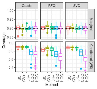
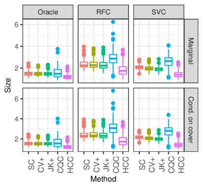
Figure 1: Several classification methods on simulated data with 10 classes, for different choices of calibration and black-box models. SC, CV+, and JK+ are applied with our new generalized inverse quantile conformity scores defined in (7). The results correspond to 100 independent experiments with 1000 training samples and 5000 test samples each. All methods have 90% marginal coverage. (a): Marginal coverage and worst-slice conditional coverage. (b): Size of prediction sets.

4 Experiments with real data

In this section, we compare the performance of our proposed methods (SC, CV+, and JK+) with the new generalized inverse quantile conformity scores defined in (7) to those of HCC and CQC [2]. We found that the original suggestion of [2] to fit a quantile neural network [21] on the class probability score can be unstable and yield very wide predictions. Therefore, we offer a second variant of this calibration method, denoted by CQC-RF, which replaces the quantile neural network estimator with quantile random forests [14]; see Supplementary Section LABEL:sec:supp-real-data for details.

The validity and statistical efficiency of each method is evaluated according to the same metrics as in Section 3. In all experiments, we set $\alpha=0.1$ and use the following base predictive models: (i) kernel SVC, (ii) random forest classifier (RFC), and (iii) two-layer neural network classifier (NNet). A detailed description of each algorithm and corresponding hyper-parameters is in Supplementary Section LABEL:sec:supp-real-data. The methods are tested on two well-known data sets: the Mice Protein Expression data set and the MNIST handwritten digit data set. The supplementary material describes the processing pipeline and discusses additional experiments on the Fashion-MNIST and CIFAR10 data sets. Supplementary Tables LABEL:tab:mice–LABEL:tab:cifar10 summarize the results of our experiments in more detail and also consider additional settings.

Figure 2 shows that all methods attain valid marginal coverage on the Mice Protein Expression data, as expected. Here, HCC, CQC, and CQC-RF fail to achieve conditional coverage, in contrast to the proposed methods (SC, CV+, JK+) based on our new conformity scores in (7). Turning to efficiency, we observe that the prediction sets of CV+ and JK+ are smaller than those of SC, and comparable in size to those of HCC. Here, the original CQC algorithm performs poorly both in terms of conditional coverage and cardinality. The CQC-RF variant is not as unstable as the original CQC, although it does not perform much better than HCC.

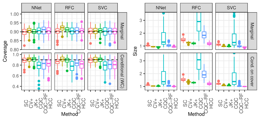
Figure 2: Experiments on Mice Protein Expression data. 100 independent experiments with 500 randomly chosen training samples and 580 test samples each. Left: coverage. Right: size of prediction sets (extremely large values for CQC not shown). Other details are as in Figure 1.

Figure 3 presents the results on the MNIST data. Here, the sample size is relatively large and hence we exclude JK+ due to its higher computational cost. As in the previous experiments, all methods achieve 90% marginal coverage. Unlike CQC, CQC-RF, and HCC, our methods also attain valid conditional coverage when relying on the NNet or SVC as base predictive models. With the RFC, all methods tend to undercover, suggesting that this classifier estimates the class probabilities poorly, and our prediction sets are larger than those constructed by CQC-RF and HCC. By contrast, the NNet enables our methods to achieve conditional coverage with prediction sets comparable in size to those produced by CQC-RF and HCC. The bottom part of Figure 3 demonstrates that CV+ also has conditional coverage given the true class label $Y$, while SC performs only slightly worse. In striking contrast, both HCC, CQC, and CQC-RF fail to achieve $90\%$ conditional coverage.

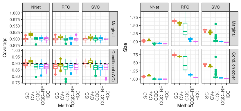
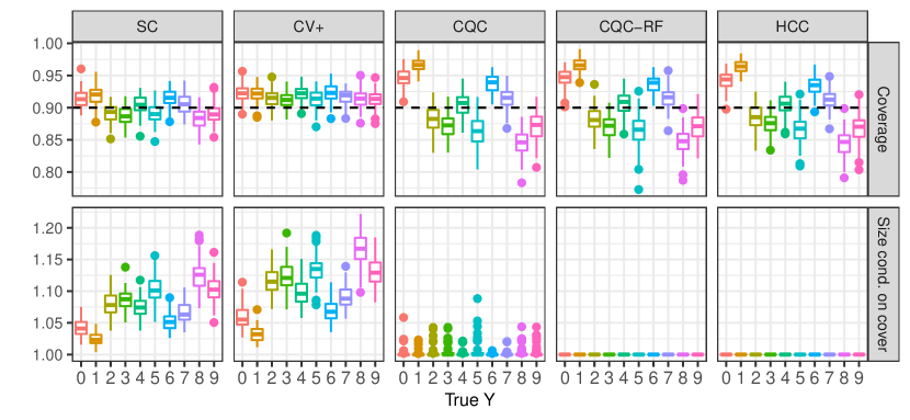
Figure 3: Experiments on MNIST data. 100 independent experiments with 10000 randomly chosen training samples and 5000 test samples each. Top: coverage and size of prediction sets (large values for CQC not shown). Bottom: coverage with neural network black box, conditional on the true $Y$, and size of the corresponding prediction sets, conditional on coverage. Other details are as in Figure 1.

5 Conclusions

This paper introduced a principled and versatile modular method for constructing prediction sets for multi-class classification problems that enjoy provable finite-sample coverage, and also behave well in terms of conditional coverage when compared to alternatives. Our approach leverages the power of any black-box machine learning classifier that may be available to practitioners, and is easily calibrated via various hold-out procedures; e.g., conformal splitting, CV+, or the jackknife+. This flexibility makes our approach widely applicable and offers options to balance between computational efficiency, data parsimony, and power.

Although this paper focused on classification, using conformity scores similar to those in (7) to calibrate hold-out procedures for regression problems [18, 4] is tantalizing. In fact, previous work in the regression setting focused on conformity scores that measure the distance of a data point from its predicted interval on the scale of the $Y$ values (which makes sense for homoscedastic regression, but may not be optimal otherwise), rather than by the amount one would need to relax the nominal threshold (our $\tau$) until the true value is covered. We leave it to future work to explore the performance of our intuitive metrics in other settings.

The Python package at https://github.com/msesia/arc implements our methods. This repository also contains code to reproduce our experiments.

Broader Impact

Machine learning algorithms are increasingly relied upon by decision makers. It is therefore crucial to combine the predictive performance of such complex machinery with practical guarantees on the reliability and uncertainty of their output. We view the calibration methods presented in this paper as an important step towards this goal. In fact, uncertainty estimation is an effective way to quantify and communicate the benefits and limitations of machine learning. Moreover, the proposed methodologies provide an attractive way to move beyond the standard prediction accuracy measure used to compare algorithms. For instance, one can compare the performance of two candidate predictors, e.g., random forest and neural network (see Figure 3), by looking at the size of the corresponding prediction sets and/or their their conditional coverage. Finally, the approximate conditional coverage that we seek in this work is highly relevant within the broader framework of fairness, as discussed by [17] within a regression setting. While our approximate conditional coverage already implicitly reduces the risk of unwanted bias, an equalized coverage requirement [17] can also be easily incorporated into our methods to explicitly avoid discrimination based on protected categories.

We conclude by emphasizing that the validity of our methods relies on the exchangeability of the data points. If this assumption is violated (e.g., with time-series data), our prediction sets may not have the right coverage. A general suggestion here is to always try to leverage specific knowledge of the data and of the application domain to judge whether the exchangeability assumption is reasonable. Finally, our data-splitting techniques in Section 4 offer a practical way to verify empirically the validity of the predictions on any given data set.

See pages - of supplement_nips.pdf

References

- [1] R. F. Barber, E. J. Candès, A. Ramdas, and R. J. Tibshirani. The limits of distribution-free conditional predictive inference. arXiv preprint arXiv:1903.04684, 2019.
- [2] M. Cauchois, S. Gupta, and J. Duchi. Knowing what you know: valid confidence sets in multiclass and multilabel prediction. arXiv preprint arXiv:2004.10181, 2020.
- [3] V. Chernozhukov, K. Wüthrich, and Y. Zhu. Distributional conformal prediction. arXiv preprint arXiv:1909.07889, 2019.
- [4] R. Foygel Barber, E. J. Candès, A. Ramdas, and R. J. Tibshirani. Predictive inference with the jackknife+. arXiv preprint arXiv:1905.02928, 2019.
- [5] L. Guan. Conformal prediction with localization. arXiv preprint arXiv:1908.08558, 2019.
- [6] C. Guo, G. Pleiss, Y. Sun, and K. Q. Weinberger. On calibration of modern neural networks. In Proceedings of the 34th International Conference on Machine Learning-Volume 70, pages 1321–1330. JMLR. org, 2017.
- [7] Y. Hechtlinger, B. Póczos, and L. Wasserman. Cautious deep learning. arXiv preprint arXiv:1805.09460, 2018.
- [8] R. Izbicki, G. T. Shimizu, and R. B. Stern. Distribution-free conditional predictive bands using density estimators. arXiv preprint arXiv:1910.05575, 2019.
- [9] D. Kivaranovic, K. D. Johnson, and H. Leeb. Adaptive, distribution-free prediction intervals for deep neural networks. arXiv preprint arXiv:1905.10634, 2019.
- [10] A. K. Kuchibhotla and A. K. Ramdas. Nested conformal prediction and the generalized jackknife+. arXiv preprint arXiv:1910.10562, 2019.
- [11] A. Kumar, P. S. Liang, and T. Ma. Verified uncertainty calibration. In Advances in Neural Information Processing Systems, pages 3787–3798, 2019.
- [12] J. Lei, M. G’Sell, A. Rinaldo, R. J. Tibshirani, and L. Wasserman. Distribution-free predictive inference for regression. Journal of the American Statistical Association, 113(523):1094–1111, 2018.
- [13] J. Lei and L. Wasserman. Distribution-free prediction bands for non-parametric regression. Journal of the Royal Statistical Society: Series B (Statistical Methodology), 76(1):71–96, 2014.
- [14] N. Meinshausen. Quantile regression forests. Journal of Machine Learning Research, 7:983–999, 2006.
- [15] L. Neumann, A. Zisserman, and A. Vedaldi. Relaxed softmax: Efficient confidence auto-calibration for safe pedestrian detection. 2018.
- [16] J. Platt. Probabilistic outputs for support vector machines and comparisons to regularized likelihood methods. Advances in large margin classifiers, 10(3):61–74, 1999.
- [17] Y. Romano, R. F. Barber, C. Sabatti, and E. Candès. With malice toward none: Assessing uncertainty via equalized coverage. Harvard Data Science Review, 4 2020. https://hdsr.mitpress.mit.edu/pub/qedrwcz3.
- [18] Y. Romano, E. Patterson, and E. J. Candès. Conformalized quantile regression. In Advances in Neural Information Processing Systems, pages 3538–3548, 2019.
- [19] M. Sadinle, J. Lei, and L. Wasserman. Least ambiguous set-valued classifiers with bounded error levels. Journal of the American Statistical Association, 114(525):223–234, 2019.
- [20] M. Sesia and E. J. Candès. A comparison of some conformal quantile regression methods. Stat, 9(1):e261, 2020.
- [21] J. W. Taylor. A quantile regression neural network approach to estimating the conditional density of multiperiod returns. Journal of Forecasting, 19(4):299–311, 2000.
- [22] J. Vaicenavicius, D. Widmann, C. Andersson, F. Lindsten, J. Roll, and T. B. Schön. Evaluating model calibration in classification. arXiv preprint arXiv:1902.06977, 2019.
- [23] V. Vovk. Conditional validity of inductive conformal predictors. In Asian conference on machine learning, pages 475–490, 2012.
- [24] V. Vovk, A. Gammerman, and G. Shafer. Algorithmic learning in a random world. Springer, 2005.
- [25] V. Vovk, D. Lindsay, I. Nouretdinov, and A. Gammerman. Mondrian confidence machine. Technical report, Royal Holloway, University of London, 2003. On-line Compression Modelling project.
- [26] V. Vovk, I. Nouretdinov, and A. Gammerman. On-line predictive linear regression. The Annals of Statistics, 37(3):1566–1590, 2009.
- [27] B. Zadrozny and C. Elkan. Obtaining calibrated probability estimates from decision trees and naive bayesian classifiers. In Icml, volume 1, pages 609–616. Citeseer, 2001.
- [28] B. Zadrozny and C. Elkan. Transforming classifier scores into accurate multiclass probability estimates. In Proceedings of the eighth ACM SIGKDD international conference on Knowledge discovery and data mining, pages 694–699, 2002.