CircleNet: Anchor-free Detection with
Circle Representation

Abstract

Object detection networks are powerful in computer vision, but not necessarily optimized for biomedical object detection. In this work, we propose CircleNet, a simple anchor-free detection method with circle representation for detection of the ball-shaped glomerulus. Different from the traditional bounding box based detection method, the bounding circle (1) reduces the degrees of freedom of detection representation, (2) is naturally rotation invariant, (3) and optimized for ball-shaped objects. The key innovation to enable this representation is the anchor-free framework with the circle detection head. We evaluate CircleNet in the context of detection of glomerulus. CircleNet increases average precision of the glomerulus detection from 0.598 to 0.647. Another key advantage is that CircleNet achieves better rotation consistency compared with bounding box representations.

1 Introduction

Detection of Glomeruli is a fundamental task for efficient diagnosis and quantitative evaluations in renal pathology. Recently, deep learning techniques have played important roles in renal pathology to reduce the clinical working load of pathologists and enable the large-scale population based research [2, 1, 6, 10, 4]. Many traditional feature-based image processing methods have been proposed for detection of glomeruli. Such methods strongly rely on “hand-crafted” features from feature engineering, such as edge detection [18], Histogram of Gradients (HOG) [8, 9, 11], median filter [13], shape features [19], Gabor filtering [5], and Hessian based Difference of Gaussians (HDoG)[25].

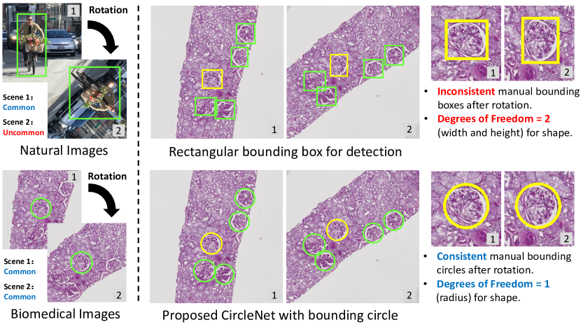
Figure 1: Comparison of rectangular bounding box and CircleNet. The left panel shows that the samples of glomeruli can be acquired and presented with any angles of rotation (both scenes are “common” for radiologist). The right panel shows that the rectangular bounding box is not optimized for the ball-shaped glomerulus. Using the proposed CircleNet, a more consistent representation with less degrees of freedom is able to be achieved.

In recent years, deep convolutional neural network (CNN) based methods have shown superior performance on detection of glomeruli with “data-driven” features. Temerinac-Ott et al. [23] proposed a glomerulus detection method by comparing the CNN performance on different stains. Gallego et al. [3] conducted glomerulus detection by integrating detection and classification, while other researchers [2, 1, 6, 10, 4] combined detection and segmentation. With the rapid development of detection technologies in computer vision, the anchor-based detection methods (e.g. Faster-RCNN [22]) have become the de facto standard glomerulus detection approach due to their superior performance. Kawazoe et al. [12] and Lo et al. [17] proposed the Faster-RCNN based method, which achieved the state-of-the-art performance on glomerulus detection. However, anchor-based methods typically yields higher model complexity and lower flexibility [22, 12] since anchors are preset on the images and refined several times as detection results. Therefore, recent academic attention has been shifted toward anchor-free detection methods (means without preset anchors) with simpler network design, less hyper parameters, and even with superior performance [14, 26, 27].

However, the “computer vision” oriented detection approaches are not necessarily optimized for biomedical objects, such as the detection of glomeruli, shown in Fig. 1. In this paper, we propose a circle representation based anchor-free detection method, called CircleNet, for robust detection of glomeruli. Briefly, the “bounding circle” is introduced as the detection representation for the ball-shaped structure of the glomerulus. After detecting the center location of the glomerulus, the DoF = 1 (radius) are required to fit the bounding circle, while the DoF = 2 (height and width) are needed for bounding box. Briefly, the contributions of this study are in three areas:

$\bullet$ Optimized Biomedical Object Detection: To the best of our knowledge, the proposed CircleNet is the first anchor-free approach for detection of glomeruli with optimized circle representation.

$\bullet$ Circle Representation: We propose a simple circle representation for ball-shaped biomedical object detection with smaller DoF of fitting and superior detection performance. We also introduce the cIOU and validate the effectiveness of both circle representation and cIOU

$\bullet$ Rotation Consistency: The proposed CircleNet achieved better rotation consistency for detection of glomeruli.

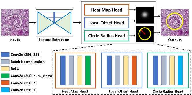
Figure 2: The network structure of proposed CircleNet. The role of the center point localization network is to achieve feature maps for the resulting head networks. Then three network heads are used to achieve the central location and the radius of a bounding circle.

2 Methods

2.1 Anchor Free Backbone

In Fig. 2, the center point localization (CPL) network is developed based on the anchor-free CenterNet implementation [26], as it possesses an ideal combination of high performance and simplicity. Throughout, we follow the definition of the terms from Zhou et al.  [26]. The input image $I$ is defined as $I\in R^{W\times H\times 3}$ with height $H$ and width $W$. The output of the CPL network is the center localization of each object, which is formed as a heatmap $\hat{Y}\in[0,1]^{\frac{W}{R}\times\frac{H}{R}\times C}$. $C$ indicates the number of candidate classes, while $R$ is the downsampling factor of the prediction. The heatmap $\hat{Y}$ is expected to be equal to $1$ at lesion centers, while $0$ otherwise. Following standard practice [14, 26], the ground truth of the target center point is modeled as a 2D Gaussian kernel:

$${Y_{xyc}=\exp\left(-\frac{(x-\tilde{p}_{x})^{2}+(y-\tilde{p}_{y})^{2}}{2\sigma_{p}^{2}}\right)}$$ (1)

where the $\tilde{p}_{x}$ and $\tilde{p}_{y}$ are the downsampled target center points and $\sigma_{p}$ is the kernel standard deviation. The predicted heatmap is optimized by pixel regression loss $L_{k}$ with focal loss [15]:

$$L_{k}=\frac{-1}{N}\sum_{xyc}\begin{cases}(1-\hat{Y}_{xyc})^{\alpha}\log(\hat{Y}_{xyc})&\!\text{if}\ Y_{xyc}=1\vspace{2mm}\\ \begin{array}[]{c}(1-Y_{xyc})^{\beta}(\hat{Y}_{xyc})^{\alpha}\\ \log(1-\hat{Y}_{xyc})\end{array}&\!\text{otherwise}\end{cases}$$ (2)

where $\alpha$ and $\beta$ are hyper-parameters in the focal loss [15]. Then, the $\ell_{1}$-norm offset prediction loss $L_{off}$, is formulated to further refine the prediction location, which is identical as [26].

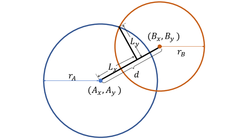
Figure 3: The parameters that are used to calculate the circle IOU (cIOU).

2.2 From Center Point to Bounding Circle

Once the peaks of the all heatmaps are obtained, the top $n$ peaks are proposed whose value is greater or equal to its 8-connected neighbors. The set of $n$ detected center points is defined as $\hat{\mathcal{P}}=\{(\hat{x}_{i},\hat{y}_{i})\}_{i=1}^{n}$. Each key point location is formed by an integer coordinate $(x_{i},y_{i})$ from $\hat{Y}_{x_{i}y_{i}c}$ and $L_{k}$. Meanwhile, the offset $(\delta\hat{x}_{i},\delta\hat{y}_{i})$ is obtained from $L_{off}$. Then, the bounding circle is formed as a circle with center point $\hat{p}$ and radius $\hat{r}$ as:

$$\hat{p}=(\hat{x}_{i}+\delta\hat{x}_{i},\ \ \hat{y}_{i}+\delta\hat{y}_{i}).\quad\hat{r}=\hat{R}_{\hat{x}_{i},\hat{y}_{i}}.$$ (3)

where $\hat{R}\in\mathcal{R}^{\frac{W}{R}\times\frac{H}{R}\times 1}$ is the radius prediction for each pixel location, optimized by

$$L_{radius}=\frac{1}{N}\sum_{k=1}^{N}\left|\hat{R}_{p_{k}}-r_{k}\right|.$$ (4)

where $r_{k}$ is the true radius for each circle object $k$. Finally, The overall objective is

$$L_{det}=L_{k}+\lambda_{radius}L_{radius}+\lambda_{off}L_{off}.$$ (5)

We set $\lambda_{radius}=0.1$ and $\lambda_{off}=1$ referring from  [26].

2.3 Circle IOU

In canonical object detection, IOU is the most popular evaluation metric to measure the similarity between two bounding boxes. The IOU is defined as the ratio between area of intersection and area of union. For CircleNet, as the objects are presented as circles, we introduce the cIOU as:

$$\textrm{cIOU}=\frac{\textrm{Area}\left(A\cap B\right)}{\textrm{Area}\left(A\cup B\right)}$$ (6)

where $A$ and $B$ represent the two circles respectively as Fig. 3. The center coordinates of $A$ and $B$ are defined as $(A_{x},A_{y})$ and $(B_{x},B_{y})$, which are calculated by:

$$A_{x}=\hat{x}_{i}+\delta\hat{x}_{i},A_{y}=\hat{y}_{i}+\delta\hat{y}_{i}$$ (7)

$$B_{x}=\hat{x}_{j}+\delta\hat{x}_{j},B_{y}=\hat{y}_{j}+\delta\hat{y}_{j}$$ (8)

Then, the distance between the center coordinates $d$ is defined as:

$$d=\sqrt{\left(B_{x}-A_{x}\right)^{2}+\left(B_{y}-A_{y}\right)^{2}}$$ (9)

$$L_{x}=\frac{r_{A}^{2}-r_{B}^{2}+d^{2}}{2d},L_{y}=\sqrt{r_{A}^{2}-L_{x}^{2}}$$ (10)

Finally, the cIOU can be calculated from

$$\textrm{Area}\left(A\cap B\right)=r_{A}^{2}\sin^{-1}\left(\frac{L_{y}}{r_{A}}\right)+r_{B}^{2}\sin^{-1}\left(\frac{L_{y}}{r_{B}}\right)-L_{y}\left(L_{x}+\sqrt{r_{A}^{2}-r_{B}^{2}+L_{x}^{2}}\right)$$ (11)

$$\textrm{Area}\left(A\cup B\right)=\pi r_{A}^{2}+\pi r_{B}^{2}-\textrm{Area}\left(A\cap B\right)$$ (12)

3 Data and Implementation Details

Whole scan images from renal biopsies were utilized for analysis. Kidney tissue was routinely processed, paraffin embedded, and 3$\mu m$ thickness sections cut and stained with hematoxylin and eosin (HE), periodic acid–Schiff (PAS) or Jones. Samples were deidentified, and studies were approved by the Institutional Review Board (IRB). 704 glomeruli from 42 biopsy samples were used as training data, 98 glomeruli from 7 biopsy samples were used as validation data, while 147 glomeruli from 7 biopsy samples were used as testing data. For all training and testing data, the original high-resolution whole scan images (0.25 $\mu m$ per pixel) is downsampled to lower resolution (4 $\mu m$ per pixel), considering the size of a glumerulus [21] and its ratio within a patch. Then, we randomly sampled image patches (each patch contained at least one glomerulus with $512\times 512$ pixels) as experimental images for detection networks. Eventually, we formed a cohort with 7040 training, 980 validation, and 1470 testing images

The Faster-RCNN [22], CornerNet [14], ExtremeNet [27], CenterNet [26] were employed as the baseline methods due to their superior performance in object detection. For different detection methods, ResNet-50 [7], stacked Hourglass-104 [20] network and deep layer aggregation (DLA) network  [24] were employed as backbone networks, respectively. The implementations of detection and backbone networks followed the authors’ official PyTorch implementations. All the models used in this study were initialized by the COCO pretrained model  [16]. The same workstation with NVIDIA 1080Ti GPU was used to perform all experiments in this study.

4 Results

Table 1: The detection performance.

Methods	Backbone	$AP\qquad$	$AP_{(50)}\quad$	$Ap_{(75)}\quad$	$Ap_{(S)}\quad$	$Ap_{(M)}$
Faster-RCNN[22]	ResNet-50	0.584	0.866	0.730	0.478	0.648
Faster-RCNN[22]	ResNet-101	0.568	0.867	0.694	0.460	0.633
CornerNet[14]	Hourglass-104	0.595	0.818	0.732	0.524	0.695
ExtremeNet[27]	Hourglass-104	0.597	0.864	0.749	0.493	0.658
CenterNet-HG[26]	Hourglass-104	0.574	0.853	0.708	0.442	0.649
CenterNet-DLA[26]	DLA	0.598	0.902	0.735	0.513	0.648
CircleNet-HG (Ours)	Hourglass-104	0.615	0.853	0.750	0.586	0.656
CircleNet-DLA (Ours)	DLA	0.647	0.907	0.787	0.597	0.685

4.1 Detection Performance

The standard detection metrics were used to evaluate different methods, including average precision ($AP$), $AP_{50}$ (IOU threshold at 0.5), $AP_{75}$ (IOU threshold at 0.75), $AP_{S}$ (small scale with area $<$ 1000), $AP_{M}$ (median scale with area $>$ 1000). In the experiment, state-of-the-art anchor-based (Faster-RCNN) and anchor-free detection methods (CornerNet, ExtremeNet, CenterNet) were employed as benchmarks. From Table.LABEL:table:detect, the proposed method outperformed the benchmarks with a remarkable margin, except for $AP_{M}$. However, the performance of the proposed method still achieved the second best performance for $AP_{M}$.

4.2 Circle Representation and cIOU

Figure 4: The ratio between the mask area and bounding box/circle area, called mask detection ratio (MDT). The masks and representations were manually traced (left and middle panel) on 50 randomly selected glomerulus from the testing cohort. As the result, the mean MDT was close across rectangular box representations and circle representations

We further evaluated if the better detection results of circle representation sacrificed the effectiveness for detection representation. To do that, we manually annotated 50 glomerulus from the testing data to achieve segmentation masks. Then, we calculated the ratio between the mask area and bounding box/circle area, called mask detection ratio (MDT), for each glomerulus. From the right panel of Fig. 4, both box and circle representations have the comparable mean MDT, which shows that the bounding circle does not sacrifice the effectiveness for detection representation.

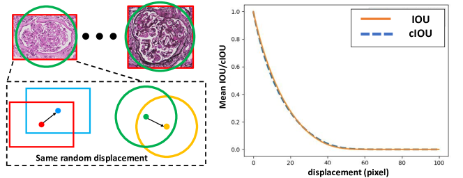
Figure 5: The effectiveness of IOU and cIOU metrics. For every testing glomerulus, we shifted the bounding box/circle with certain displacement in a random direction (left panel). Then, the IOU and cIOU values between the original and shifted bounding boxes/circles were calculated for different displacement (right panel).

For bounding box and bounding circle, the IOU and cIOU were used as the overlap metrics for evaluating the detection performance (e.g., $AP_{50}$ and $AP_{75}$) between manual annotations and predictions. Herein, we compared the performance of bounding box and bounding circle as similarity metrics for detection of glomeruli. To test this, we added random displacements with random directions on all testing glomeruli to simulate different detection results. Then, we calculated the IOU and cIOU, respectively. Fig. 5 presents the results of mean IOU and mean cIOU on all testing glomeruli, with the displacements varying from 0 to 100 pixels. The results show that the cIOU behaves nearly the same as a IOU, which shows that the cIOU is a validated overlap metrics for detection of glomeruli.

4.3 Rotation Consistency

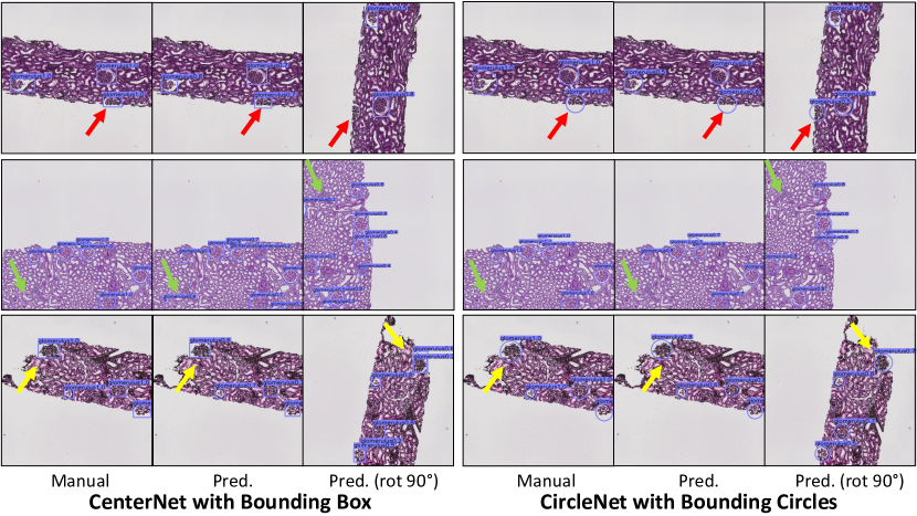
Figure 6: The qualitative results of detection and rotation consistency. Each row indicates a different example patches. The arrows indicate the inconsistent detection results in different cases.

Another potential benefit for circle representation is better rotation consistency than rectangular boxes. As shown in Fig. 6, we evaluated the consistency of bounding box/circle detection by rotating the original testing images. To avoid the impact from intensity interpolation, we rotated the original image 90 degrees rather than an arbitrary degree. By doing this, detected bounding box/circle on rotated images were conveniently able to be converted to the original space. To fairly compare the rotation consistency, the rotation was only applied during testing stage. Therefore, we did not apply any rotation as data augmentation during training for all methods. The consistency was calculated by dividing the number of overlapped bounding boxes/circles (IOU or cIOU $>$ 0.5 before and after rotation) by the average number of total detected bounding boxes/circles (before and after rotation). The percentage of overlapped detection was named “rotation consistency” ratio, where 0 means no overlapped boxes/circles after rotation and 1 means all boxes/circles overlapped. Table LABEL:table:overlap shows the rotation consistency results with traditional bounding box representation and bounding circle representation. The proposed CircleNet-DLA approach achieved the best rotation consistency. One explanation of the better performance would be that the radii are naturally spatial invariant metrics, while the length and width metrics are sensitive to rotation.

Table 2: Rotation consistency results of bounding box and bounding circle.

Representation	Methods	Backbone	Rotation Consistency
Bounding Box	CenterNet-HG[26]	Hourglass-104	0.833
Bounding Box	CenterNet-DLA[26]	DLA	0.851
Bounding Circle	CircleNet-HG (Ours)	Hourglass-104	0.875
Bounding Circle	CircleNet-DLA (Ours)	DLA	0.886

5 Conclusion

In this paper, we introduce CircleNet, an anchor-free method for detection of glomeruli. The proposed detection method is optimized for ball-shaped biomedical objects, with the superior detection performance and better rotation consistency. The new circle representation as well as the cIOU evaluation metric were comprehensively evaluated in this study. The results show that the circle representation does not sacrifice the effectiveness with less DoF compared with traditional representation for detection of glomeruli.

6 Acknowledgement

This work was supported by NIH NIDDK DK56942(ABF), NSF CAREER 1452485 (Landman).

References

- [1] Bueno, G., Fernandez-Carrobles, M.M., Gonzalez-Lopez, L., Deniz, O.: Glomerulosclerosis identification in whole slide images using semantic segmentation. Computer Methods and Programs in Biomedicine 184, 105273 (2020)
- [2] Gadermayr, M., Dombrowski, A.K., Klinkhammer, B.M., Boor, P., Merhof, D.: Cnn cascades for segmenting whole slide images of the kidney. arXiv preprint arXiv:1708.00251 (2017)
- [3] Gallego, J., Pedraza, A., Lopez, S., Steiner, G., Gonzalez, L., Laurinavicius, A., Bueno, G.: Glomerulus classification and detection based on convolutional neural networks. Journal of Imaging 4(1), 20 (2018)
- [4] Ginley, B., Lutnick, B., Jen, K.Y., Fogo, A.B., Jain, S., Rosenberg, A., Walavalkar, V., Wilding, G., Tomaszewski, J.E., Yacoub, R., et al.: Computational segmentation and classification of diabetic glomerulosclerosis. Journal of the American Society of Nephrology 30(10), 1953–1967 (2019)
- [5] Ginley, B., Tomaszewski, J.E., Yacoub, R., Chen, F., Sarder, P.: Unsupervised labeling of glomerular boundaries using gabor filters and statistical testing in renal histology. Journal of Medical Imaging 4(2), 021102 (2017)
- [6] Govind, D., Ginley, B., Lutnick, B., Tomaszewski, J.E., Sarder, P.: Glomerular detection and segmentation from multimodal microscopy images using a butterworth band-pass filter. In: Medical Imaging 2018: Digital Pathology. vol. 10581, p. 1058114. International Society for Optics and Photonics (2018)
- [7] He, K., Zhang, X., Ren, S., Sun, J.: Deep residual learning for image recognition. In: Proceedings of the IEEE conference on computer vision and pattern recognition. pp. 770–778 (2016)
- [8] Kakimoto, T., Okada, K., Hirohashi, Y., Relator, R., Kawai, M., Iguchi, T., Fujitaka, K., Nishio, M., Kato, T., Fukunari, A., et al.: Automated image analysis of a glomerular injury marker desmin in spontaneously diabetic torii rats treated with losartan. The Journal of endocrinology 222(1), 43 (2014)
- [9] Kakimoto, T., Okada, K., Fujitaka, K., Nishio, M., Kato, T., Fukunari, A., Utsumi, H.: Quantitative analysis of markers of podocyte injury in the rat puromycin aminonucleoside nephropathy model. Experimental and Toxicologic Pathology 67(2), 171–177 (2015)
- [10] Kannan, S., Morgan, L.A., Liang, B., Cheung, M.G., Lin, C.Q., Mun, D., Nader, R.G., Belghasem, M.E., Henderson, J.M., Francis, J.M., et al.: Segmentation of glomeruli within trichrome images using deep learning. Kidney international reports 4(7), 955–962 (2019)
- [11] Kato, T., Relator, R., Ngouv, H., Hirohashi, Y., Takaki, O., Kakimoto, T., Okada, K.: Segmental hog: new descriptor for glomerulus detection in kidney microscopy image. Bmc Bioinformatics 16(1), 316 (2015)
- [12] Kawazoe, Y., Shimamoto, K., Yamaguchi, R., Shintani-Domoto, Y., Uozaki, H., Fukayama, M., Ohe, K.: Faster r-cnn-based glomerular detection in multistained human whole slide images. Journal of Imaging 4(7), 91 (2018)
- [13] Kotyk, T., Dey, N., Ashour, A.S., Balas-Timar, D., Chakraborty, S., Ashour, A.S., Tavares, J.M.R.: Measurement of glomerulus diameter and bowman’s space width of renal albino rats. Computer methods and programs in biomedicine 126, 143–153 (2016)
- [14] Law, H., Deng, J.: Cornernet: Detecting objects as paired keypoints. In: Proceedings of the European Conference on Computer Vision (ECCV). pp. 734–750 (2018)
- [15] Lin, T.Y., Goyal, P., Girshick, R., He, K., Dollár, P.: Focal loss for dense object detection. In: Proceedings of the IEEE international conference on computer vision. pp. 2980–2988 (2017)
- [16] Lin, T.Y., Maire, M., Belongie, S., Hays, J., Perona, P., Ramanan, D., Dollár, P., Zitnick, C.L.: Microsoft coco: Common objects in context. In: European conference on computer vision. pp. 740–755. Springer (2014)
- [17] Lo, Y.C., Juang, C.F., Chung, I.F., Guo, S.N., Huang, M.L., Wen, M.C., Lin, C.J., Lin, H.Y.: Glomerulus detection on light microscopic images of renal pathology with the faster r-cnn. In: International Conference on Neural Information Processing. pp. 369–377. Springer (2018)
- [18] Ma, J., Zhang, J., Hu, J.: Glomerulus extraction by using genetic algorithm for edge patching. In: 2009 IEEE Congress on Evolutionary Computation. pp. 2474–2479. IEEE (2009)
- [19] Marée, R., Dallongeville, S., Olivo-Marin, J.C., Meas-Yedid, V.: An approach for detection of glomeruli in multisite digital pathology. In: 2016 IEEE 13th International Symposium on Biomedical Imaging (ISBI). pp. 1033–1036. IEEE (2016)
- [20] Newell, A., Yang, K., Deng, J.: Stacked hourglass networks for human pose estimation. In: European conference on computer vision. pp. 483–499. Springer (2016)
- [21] Puelles, V.G., Hoy, W.E., Hughson, M.D., Diouf, B., Douglas-Denton, R.N., Bertram, J.F.: Glomerular number and size variability and risk for kidney disease. Current opinion in nephrology and hypertension 20(1), 7–15 (2011)
- [22] Ren, S., He, K., Girshick, R., Sun, J.: Faster r-cnn: Towards real-time object detection with region proposal networks. In: Advances in neural information processing systems. pp. 91–99 (2015)
- [23] Temerinac-Ott, M., Forestier, G., Schmitz, J., Hermsen, M., Bräsen, J., Feuerhake, F., Wemmert, C.: Detection of glomeruli in renal pathology by mutual comparison of multiple staining modalities. In: Proceedings of the 10th International Symposium on Image and Signal Processing and Analysis. pp. 19–24. IEEE (2017)
- [24] Yu, F., Wang, D., Shelhamer, E., Darrell, T.: Deep layer aggregation. In: Proceedings of the IEEE conference on computer vision and pattern recognition. pp. 2403–2412 (2018)
- [25] Zhang, M., Wu, T., Bennett, K.M.: A novel hessian based algorithm for rat kidney glomerulus detection in 3d mri. In: Medical Imaging 2015: Image Processing. vol. 9413, p. 94132N. International Society for Optics and Photonics (2015)
- [26] Zhou, X., Wang, D., Krähenbühl, P.: Objects as points. arXiv preprint arXiv:1904.07850 (2019)
- [27] Zhou, X., Zhuo, J., Krahenbuhl, P.: Bottom-up object detection by grouping extreme and center points. In: Proceedings of the IEEE Conference on Computer Vision and Pattern Recognition. pp. 850–859 (2019)