Interacting quantum Hall states in a finite graphene flake and at finite temperature

Abstract

The integer quantum Hall states at fillings $\nu=0$ and $|\nu|=1$ in monolayer graphene have drawn much attention as they are generated by electron-electron interactions. Here we explore aspects of the $\nu=0$ and $|\nu|=1$ quantum Hall states relevant for experimental samples. In particular, we study the effects of finite extent and finite temperature on the $\nu=0$ state and finite temperature for the $\nu=1$ state. For the $\nu=0$ state we consider the situation in which the bulk is a canted antiferromagnet and use parameters consistent with measurements of the bulk gap to study the edge states in tilted magnetic fields in order to compare with experiment [A. F. Young et al., Nature 505, 528 (2014)]. When spatial modulation of the order parameters is taken into account, we find that for graphene placed on boron nitride, the gap at the edge closes for magnetic fields comparable to those in experiment, giving rise to edge conduction with $G\sim 2e^{2}/h$ while the bulk gap remains almost unchanged. We also study the transition into the ordered state at finite temperature and field. We determine the scaling of critical temperatures as a function of magnetic field, $B$, and distance to the zero field critical point and find sublinear scaling with magnetic field for weak and intermediate strength interactions, and $\sqrt{B}$ scaling at the coupling associated with the zero field quantum critical point. We also predict that critical temperatures for $\nu=0$ states should be an order of magnitude higher than those for $|\nu|=1$ states, consistent with the fact that the low temperature gap for $\nu=0$ is roughly an order of magnitude larger than that for $|\nu|=1$.

I Introduction

The quantum Hall states in monolayer graphene reflect the Dirac nature of the low energy quasiparticles, exhibiting plateaux for $\nu=\pm(4n+2)$ at weak magnetic fields qhe-graphene-1 ; qhe-graphene-2 . In a non-interacting picture the positions of these plateaux can be understood as arising from fourfold valley and spin degeneracy of two dimensional Dirac fermions sharapov . At stronger magnetic fields, additional plateaux arise at $\nu=0,\pm 1$ and $\pm 4$ Zhang2007 . The $\nu=0$ quantum Hall state in particular has attracted much recent experimental Zhang2007 ; Andrei2010 ; YacobyPRB2013 ; NovoselovPNAS ; Young2012 ; Andrei2009 ; Dean2011 ; Yacoby2012 ; Li2019 ; Hong2019 and theoretical Roy2014 ; Khveshchenko2001 ; HerbutPRL2006 ; HJR2009 ; herbut-qhe ; herbut2007 ; KunYang2007 ; semenoff-zhou ; barlas-review ; kharitonov ; Narayanan2018 ; goerbig-review attention as it is an example of an integer quantum Hall state that is generated by electron-electron interactions.

In a strong magnetic field, electron-electron interactions are enhanced as kinetic energy is quenched by the formation of Landau levels (LLs) which can lead to the formation of ordered phases even for infinitesimally small interactions in the presence of a magnetic field, not only by splitting the half-filled zeroth LL (ZLL), but also by simultaneously lowering the energies of all filled LLs with negative energies. This phenomenon is known as magnetic catalysis Roy2014 ; herbut-qhe ; herbut2007 ; roy-scaling ; roy-inhomogeneous-catalysis ; Shovkovy2013 ; Tada2020 ; Gorbar2002 ; catalysis-original . The ZLL is distinct from other LLs in monolayer graphene as it is simultaneously valley and sublattice polarized. There have been numerous suggestions for broken symmetry phases that can cause splitting of the ZLL and give rise to a $\nu=0$ quantum Hall effect dassarma-yang-macdonald ; moessner ; fuchs ; nomura-macdonald ; herbut-qhe ; herbut2007 ; Jung2009 ; semenoff-zhou ; gusynin-miransky-PRB ; barlas-review ; kharitonov ; Roy2014 . In Ref. Roy2014 , two of us argued that chiral symmetry breaking orders, i.e. orders that break the sublattice symmetry (e.g. antiferromagnetism or charge density wave orders), are likely to be favoured when one considers the effect of ordering on all filled LLs, not just the ZLL. Subsequently, the importance of considering multiple filled LLs was also emphasised in Refs. Feshami2016 ; Lukose2016 . Such symmetry breaking orders can occur for electrons on a honeycomb lattice for sufficiently strong short-range interactions HerbutPRL2006 ; HJR2009 , however, in graphene the strength of these interactions are not sufficient to induce order in the absence of a magnetic field katsnelson . By solving mean field gap equations that include the mixing of the filled LLs (also known as LL mixing) when chiral symmetry breaking orders are present, we obtained an excellent fit of the excitation gap as a function of perpendicular magnetic field Roy2014 obtained by several different experimental groups YacobyPRB2013 ; NovoselovPNAS ; Young2012 .

There are a number of terms in the Hamiltonian that give rise to orders that compete to give the ground state in the $\nu=0$ state. Antiferromagnetism can arise from short range Hubbard interactions HerbutPRL2006 ; HJR2009 , and competes with ferromagnetic ordering arising from the Zeeman coupling of the magnetic field to spin. The antiferromagnetic order is controlled by the magnetic field perpendicular to the graphene sheet, while the Zeeman coupling scales with the total magnetic field. Hence, it is to be expected that increasing the total field at fixed perpendicular magnetic field should lead to a transition from an antiferromagnetic to a ferromagnetic state kharitonov .

The competition between different states can be affected by the finite extent and temperature of the sample. In the case of either an antiferromagnet or a ferromagnet, both phases are gapped in the bulk, but can be distinguished by their edge states – a purely ferromagnetic state in the ZLL of graphene has gapless edge modes giving Hall conductivity $\sigma_{xy}=2e^{2}/h$ abanin-edge ; FertigBrey2006 , whereas an easy-plane antiferromagnet has gapped edge states. There have been several transport experiments on graphene in a tilted field Young2012 ; Young2014 , which have demonstrated that the edge conductance in the $\nu=0$ state changes from $G=0$ to $G\simeq 2e^{2}/h$ with increasing parallel magnetic field Young2014 , and this has been interpreted as a transition from an antiferromagnetic state to a ferromagnetic state. These considerations have spurred theoretical investigations of edge states for the $\nu=0$ quantum Hall state Jung2009 ; kharitonov ; Lado2014 ; Murthy2014 ; Knothe2015 ; HuangCazalilla2015 ; Piyatkovskiy2014 ; Tikhonov2016 ; Murthy2016 ; miransky-edge ; Gusynin2009 . We now present a summary of our main findings.

I.1 Summary of Results

The presence of an edge will generically affect the spatial profile of the order parameter near the edge. Studies of $\nu=0$ quantum Hall edges have either calculated edge states using bulk order parameters kharitonov ; Piyatkovskiy2014 or allowed for the spatial variation of order parameters in the vicinity of the edge Jung2009 ; Lado2014 ; Murthy2016 ; Tikhonov2016 ; Knothe2015 ; Murthy2014 ; HuangCazalilla2015 . The relationship between ordering in the bulk and ordering in the vicinity of the edge has not yet been quantitatively compared with experiment. In this paper we extend the approach used to obtain quantitative agreement with bulk measurements in Ref. Roy2014 and apply it to consider measurements of edge transport reported by Young et al. Young2014 . In particular, we use the magnetic field dependence for the bulk gaps obtained in Ref. Roy2014 as input for calculations of edge states. We first calculate edge states ignoring spatial variation of the order parameter, and determine the behaviour of the states and gaps as a function of tilted field (shown in Fig. 4). These results are in qualitative but not quantitative agreement with experiment, motivating us to consider the effect of spatial variations of the order parameters in the presence of an edge. We include these spatial variations phenomenologically, using a profile for the order parameters based on the results of Ref. Lado2014 , and find that for a graphene flake on a substrate placed in a perpendicular field $B_{\perp}=0.7$ T, the gap at the edge closes for a parallel field of $B_{\parallel}\sim 40$ T, in reasonable agreement with experiment Young2014 . Therefore, chiral symmetry breaking orderings within the framework of magnetic catalysis provide a good description of both the bulk and the edge of the $\nu=0$ quantum Hall state.

We also consider thermal corrections to the gap equations solved in Ref. Roy2014 . This allows us to obtain estimates for the critical temperature for the $\nu=0$ and $|\nu|=1$ quantum Hall states. Our estimates are comparable with experimental observations, with the transition in the $\nu=0$ state taking place at about ten times higher temperature scales than for the $|\nu|=1$ states. We obtain the scaling of the critical temperature with magnetic field and distance to the zero field critical point (shown in Figs. 9 and 11), and find that the exponent of the magnetic field dependence appears to have a simple relation to the distance to the zero field critical point. Overall, the scaling of the transition temperature ($T_{c}$) with the magnetic field follows closely that of the corresponding chiral symmetry breaking mass at zero temperature roy-scaling ; roy-inhomogeneous-catalysis . In particular, $T_{c}$ respectively scales linearly and sublinearly for weak and intermediate subcritical interaction strengths, while for the zero field critical interaction strength $T_{c}\sim\sqrt{B}$.

I.2 Organization

This paper is structured as follows. In Sec. II we review the solution of edge states obtained using bulk values of the order parameters and show numerical results based on values appropriate to fit the results of experiments on the bulk. In Sec. III we calculate edge states allowing for spatial variation of the order parameters and in Sec. IV we consider the effects of thermal fluctuations on the bulk gaps. Finally, in Sec. V we discuss our results and conclude.

II Edge States

In this section we briefly review the low energy theory of graphene in a strong magnetic field and the calculation of edge states in the presence of in-plane antiferromagnetic and easy-axis ferromagnetic order parameters. These orders can arise due to the presence of short range interactions between electrons HerbutPRL2006 ; HJR2009 . We consider the order parameters to be spatially uniform (a condition that will be relaxed in Sec. III) and study their evolution under a tilted magnetic field using experimentally relevant parameter values. If the spatial variation of the order parameters is sufficiently weak that their value close to the edge is similar to their bulk value, then this should be a good approximation. We present these results as a point of reference for more careful comparison with experiment.

II.1 Model

The low energy theory of monolayer graphene can be constructed from fermions residing in the valleys centred on the two inequivalent Dirac points $\pm\,{\mathbf{K}}$ at the corners of the Brillouin zone. The states may be written using an eight component spinor $\Psi=[\Psi_{\uparrow},\Psi_{\downarrow}]^{T}$, where $\Psi_{\sigma}^{T}=[u_{\sigma}(+{\mathbf{K}}+{\mathbf{q}}),v_{\sigma}(+{\mathbf{K}}+{\mathbf{q}}),u_{\sigma}(-{\mathbf{K}}+{\mathbf{q}}),v_{\sigma}(-{\mathbf{K}}+{\mathbf{q}})],$ with $|{\mathbf{q}}|\ll|{\mathbf{K}}|$ and $u_{\sigma}$ and $v_{\sigma}$ are fermionic annihilation operators on the two sublattices of the honeycomb lattice and $\sigma=$ $\uparrow$ or $\downarrow$ labels electron spin. The effective Dirac dispersion applies out to an ultraviolet momentum cutoff $\Lambda$ which is of order $1/a$, where $a$ is the lattice spacing.

Figure 1: Boundary conditions for a finite graphene sheet, with zigzag and armchair edges illustrated.

In this basis the Hamiltonian has the structure ${\rm spin}\otimes{\rm valley}\otimes{\rm sublattice}$ and allowing for both antiferromagnetic and ferromagnetic ordering the Hamiltonian takes the form herbut2007

$$H=I_{2}\otimes H_{0}-\left({\mathbf{N}}\cdot\mbox{\boldmath$\sigma$}\right)\otimes\gamma_{0}+\left(\lambda+m_{3}\right)\sigma_{3}\otimes I_{4},$$

where $H_{0}=i\gamma_{0}\gamma_{j}\left(-i\partial_{j}-A_{j}\right)$ (using the Einstein summation convention), and the gamma matrices take the form $\gamma_{0}=I_{2}\otimes\sigma_{3}$, $\gamma_{1}=\sigma_{3}\otimes\sigma_{2}$, $\gamma_{2}=-I_{2}\otimes\sigma_{1}$, $\gamma_{3}=\sigma_{1}\otimes\sigma_{2}$, and $\gamma_{5}=\sigma_{2}\otimes\sigma_{2}$, where the $\sigma_{i}$ are the usual Pauli matrices. We use units with $e$, $\hbar$ and $v_{F}$ set to unity unless otherwise specified. The parameter $\lambda=g\mu_{B}B$ is the Zeeman coupling and ${\mathbf{N}}$ and ${\mathbf{m}}$ are the Néel and ferromagnetic order parameters respectively. These order parameters arise from representing the short range part of electron-electron interactions with a repulsive on-site Hubbard term

$$H_{U}=\frac{U}{2}\sum_{i}n_{i\uparrow}n_{i_{\downarrow}},$$ (1)

and decomposing it with a mean-field approximation herbut2007 ; Roy2014 . We focus on these two orders as they appear to be the most relevant for the $\nu=0$ quantum Hall state kharitonov ; Roy2014 . Similarly to Ref. herbut2007 we exchange the valley and spin indices so that the Hamiltonian is block diagonal in the valley index:

$$H=H_{+}\oplus H_{-},$$ (2)

where $H_{\pm}$ refers to the $\pm K$ valley and $H_{+}$ and $H_{-}$ are related to the Hamiltonian

$${\mathcal{H}} = H_{0}+i\gamma_{0}\gamma_{3}N_{1}+i\gamma_{0}\gamma_{5}N_{2}+i\gamma_{3}\gamma_{5}(\lambda+m),$$ (3)

via unitary transformations. We define $N_{1}$ and $N_{2}$ as the $x$ and $y$ components of the antiferromagnetic order parameter and $m$ as the magnitude of the ferromagnetic order parameter. Specifically, $H_{+}=U_{1}^{\dagger}{\mathcal{H}}U_{1}$ where $U_{1}=I_{2}\oplus i\sigma_{2}$ and $H_{-}=U_{2}^{\dagger}{\mathcal{H}}U_{2}$ where $U_{2}=i\sigma_{2}\oplus I_{2}$. The eight component spinor is transformed to $\Psi=[\Psi_{+},\Psi_{-}]^{T}$, where $\Psi_{\pm}=[u_{\uparrow}(\pm{\mathbf{K}}+{\mathbf{q}}),v_{\uparrow}(\pm{\mathbf{K}}+{\mathbf{q}}),u_{\downarrow}(\pm{\mathbf{K}}+{\mathbf{q}}),v_{\downarrow}(\pm{\mathbf{K}}+{\mathbf{q}})]^{T}$.

We follow a similar approach to calculating the edge states to Pyatkovskiy and Miransky Piyatkovskiy2014 . We consider a half-plane in which boundary conditions are imposed on one edge and the condition of normalizability is also applied. We focus on armchair edges which are illustrated along with zigzag edges in Fig. 1, and details of our calculations are provided in Appendix A.

The spectrum can be written as

$$E_{\sigma}=\pm\sqrt{{\mathcal{N}}_{\perp}^{2}+\left[(\tilde{\lambda}+\tilde{m})+\sigma\sqrt{-\Omega-1}\right]^{2}},$$ (4)

where ${\mathcal{N}}_{\perp}^{2}=(N_{1}^{2}+N_{2}^{2})/B$, $\tilde{\lambda}=\lambda/\sqrt{B}$, $\tilde{m}=m/\sqrt{B}$, $\sigma=\pm 1$, and $\Omega$ can be found by solving an eigenvalue equation for parabolic cylinder functions that describe the edge states for the appropriate boundary condition. The details of these solutions are discussed in Appendix A, and in the limit of an infinite sheet Eq. (4) reduces to

$$E_{\sigma}=\pm\sqrt{{\mathcal{N}}_{\perp}^{2}+\left[(\tilde{\lambda}+\tilde{m})+\sigma\sqrt{2n}\right]^{2}},$$ (5)

in agreement with the expected bulk expression Roy2014 . The edge states for zigzag boundary conditions are similar, but have some differences from those for armchair boundary conditions. Specifically, for zigzag boundary conditions there are zero energy dispersionless states, which are not present for armchair boundary conditions. We now present numerical results for the edge states.

II.2 Numerical Results

As noted above, several other authors kharitonov ; Piyatkovskiy2014 ; Gusynin2009 have previously obtained the eigenvalue spectrum in the presence of edges assuming a uniform order parameter. In the work here we test whether this can be done in a quantitative manner or not by utilizing the work of Roy et al. Roy2014 , in which it was found that by solving two mean field gap equations with two adjustable parameters, quantitative agreement could be obtained between measurements of the gap as a function of perpendicular magnetic field for both suspended graphene and graphene on a substrate. In particular, we use order parameters obtained by solving the gap equation for the bulk as in Ref. Roy2014 as input to the eigenvalue equation Eq. (4). We then study the effect of a tilted magnetic field on the spectrum, focusing particularly on the gap at the edge, mirroring the situation in experiments described in Ref. Young2014 .

In Appendix B we briefly review the formalism for self-consistent gap equations in the bulk. The total gap for the $\nu=0$ Hall state in the presence of canted antiferromagnetic (CAF) order is $\Delta_{0}=\sqrt{N^{2}_{\perp}+(\lambda+m)^{2}}$, where $N_{\perp}^{2}=N_{1}^{2}+N_{2}^{2}$. The gap equations are solved numerically to find $N_{\perp}$, $m$ and $\Delta_{0}$ as a function of magnetic field as the parameters $\delta_{a}$ and $\delta_{f}$ are varied. Results are presented in terms of the cutoff energy scale $E_{c}=\hbar v_{F}\Lambda\simeq 1$ eV. Physically, $\delta_{a}$ is the distance between the critical coupling for AFM order and the actual value of the coupling and $\delta_{f}$ is the dimensionless coupling for FM order. Explicit expressions for $\delta_{a}$ and $\delta_{f}$ are presented in Appendix B. A positive value of $\delta_{a}$ corresponds to a subcritical coupling. We note that there was an error in the reported value of $\delta_{f}$ obtained in fits to experimental data in Ref. Roy2014 which does not affect other conclusions in that work footnote_Roy as the ferromagnetic order has minimal impact of the overall quality of the fit in a perpendicular magnetic field.

II.2.1 Edge states in a parallel magnetic field

The size of the bulk gap obtained from the self-consistent approach depends on the nature of the substrate, with smaller $\delta_{a}$ values (and a larger gap) for suspended graphene than for graphene placed on a substrate where screening increases $\delta_{a}$ Roy2014 and decreases the gap. Experimentally the transition from antiferromagnetism to ferromagnetism is realized by applying a magnetic field parallel to the graphene sheet.

In Fig. 2 we show the total gap ($\Delta$), ferromagnetic order parameter ($m$) and antiferromagnetic order parameter ($N_{\perp}$) as a function of parallel magnetic field for a perpendicular magnetic field of $B_{\perp}=0.14$ T for $\delta_{a}$ and $\delta_{f}$ values corresponding to suspended graphene Yacoby2012 and graphene on a substrate Young2012 . We see that graphene on a substrate is susceptible to ferromagnetism at much smaller values of $B_{\parallel}$ than suspended graphene at the same value of $B_{\perp}$. In the experiments in Ref. Young2012 , the graphene was placed on boron nitride (BN), so for Figs. 3 onward we only show results with $\delta_{a}=0.225$, $\delta_{f}=1.0$, which are representative parameter values for graphene on a BN substrate Roy2014 .

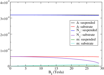
Figure 2: Order parameters in a tilted field for $B_{\perp}=0.14$ T for a suspended sample ($\delta_{a}=0.035$) and a sample on a substrate ($\delta_{a}=0.225$). In both cases the order parameters are assumed to be spatially uniform in the graphene sheet and $\delta_{f}=1.0$. Here $\Delta$, $N_{\perp}$ and $m$ are measured in units of $E_{c}=\hbar v_{F}\Lambda$.

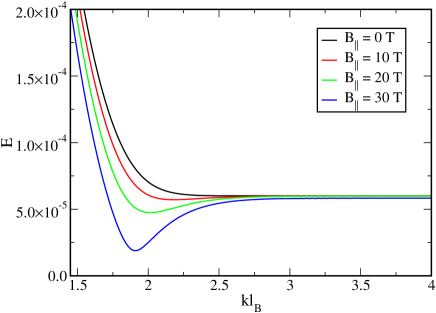
Figure 3: Energy of edge states in units of $E_{c}$ as a function of $kl_{B}$ for $B_{\perp}=0.14$ T at several different values of parallel magnetic field for an armchair boundary condition and parameters suitable for graphene on a substrate (i.e. the same as Fig. 2 (b)). The order parameters are assumed to be spatially uniform in the graphene sheet.

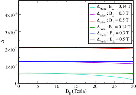
Figure 4: Comparison of the edge gap ($\Delta_{\rm edge}$) and bulk gap ($\Delta_{\rm bulk}$) as a function of parallel magnetic field for $B_{\perp}=0.14$ T, 0.3 T and 0.5 T, for an armchair edge and parameters appropriate for a substrate (i.e. the same as Fig. 2 (b)). The gaps are measured in units of $E_{c}$.

As detailed in Appendix A, we use the Landau gauge ${\mathbf{A}}=(0,Bx)$ for armchair boundary conditions and take $\Psi(x,y)=e^{iky}\Psi(x)$. In Fig. 3 we show the spectrum of edge states for armchair boundary conditions when $B_{\perp}=0.14$ T and for parallel fields ranging from $B_{\parallel}$ = 0 to 30 T. The energy of the edge states is plotted as a function of $kl_{B}$, where $l_{B}=\sqrt{\hbar/eB}$ is the magnetic length and in the infinite system size limit, $kl_{B}$ corresponds to the centre of the Gaussian part of $\Psi(x)$. One can see that for a parallel field of 30 T, the gap at the edge is substantially reduced relative to the bulk.

The evolution of the edge gap, $\Delta_{\rm edge}$, (and its relation to the bulk gap, $\Delta_{\rm bulk}$) in the $\nu=0$ state for graphene on a substrate for several different values of $B_{\perp}$ is shown in Fig. 4, and demonstrates that the required field scale for $B_{\parallel}$ to quench antiferromagnetism is much larger than 30 T for $B_{\perp}\gtrsim 0.3$ T.

The behaviour captured in Figs. 2 to 4 is in good qualitative agreement with the experimental results obtained by Young et al. Young2014 , but not in good quantitative agreement. In Ref. Young2014, , a field scale of $B_{\parallel}\sim 35$ T was required to obtain saturation of the conductance at around $G\simeq 1.8e^{2}/h$ for a sample with $B_{\perp}=1.4$ T on a BN substrate. This is suggestive of a transition to ferromagnetism at this field scale. Assuming the bulk values of the order parameters all the way out to the edge leads us to require a perpendicular field scale about 10 times smaller than experiment to see the same closing of the gap at the edge. This suggests that the size of the gap at the edge is being overestimated, and that assuming spatially uniform order parameters is an oversimplification.

III Edge states for spatially varying order parameters

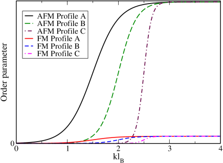
Figure 5: Phenomenological profiles of the antiferromagnetic (AFM) and ferromagnetic (FM) order parameters for an armchair edge for three different sigmoidal edge profiles. The order parameters are shown to have relative magnitudes appropriate for parameter values $\delta_{a}=0.225$, $\delta_{f}=1$ and $B_{\perp}=0.14$ T. Profile A decays between $kl_{B}$ = 2 and 3. Profile B decays between $kl_{B}$ = 1 and 3 and Profile C decays between $kl_{B}$ = 0 and 3. The order parameters take their bulk values (see Fig. 2) for $kl_{B}\geq 3$. We do not include a vertical scale as we wish to draw attention to the shape rather than the magnitude (which is fixed by the bulk gap) of the profiles.

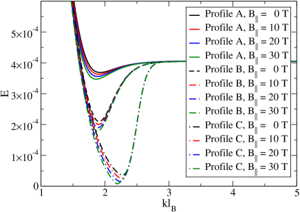
Figure 6: Spectrum in the presence of spatially varying order parameters for armchair boundary conditions with $B_{\perp}=1.4$ T for the profiles A, B, and C introduced in Fig. 5. Energies are measured in units of $E_{c}$.

Having seen in Sec. II.2.1 that assuming that the order parameters are uniform in the bulk gives a qualitatively but not quantitatively correct description of edge states in a parallel magnetic field, we generalize our discussion to allow the spatial dependence of order parameters in the presence of an edge. We do this by allowing $N$ and $m$ to be functions of $k$, i.e. $N_{k}$ and $m_{k}$, in addition to $\Omega$ which is already a function of $k$. In general, finding a self-consistent solution for $N_{k}$ and $m_{k}$ by using a similar approach to the one we used for the bulk is a very challenging problem. We expect that the general behaviour of both $N$ and $m$ is that they will decay from their bulk value in the vicinity of the edge. One could envisage generalizing the gap equation approach we use for the bulk by allowing spatial variation of order parameters. This leads to a situation where at each value of $k$, one needs to self-consistently solve for both the order parameters and $\Omega_{k}$, which involves performing sums over many filled states (which are more complicated in their energy dispersion than Landau levels), and also carefully devising an appropriate regularization procedure. Given that a spatially uniform order parameter profile already produced a qualitatively correct picture that is compatible with experiment, as a first step towards quantitative agreement, we only account for spatial variations of the order parameters phenomenologically. We make a “local density approximation”, in which we write the energy eigenvalues for a given $k$ as

$$E_{n{\mathbf{s}}}(k)=\pm\sqrt{{{\mathcal{N}}_{\perp}}_{k}^{2}+\left[(\tilde{\lambda}+\tilde{m}_{k})+\sigma\sqrt{-\Omega_{n{\mathbf{s}}}(k)-1}\right]^{2}}.$$

(6)

Rather than explicitly solving for ${N_{\perp}}_{k}$ and $m_{k}$, we assume that they have a spatial profile of the form determined by Lado and Fernández-Rossier Lado2014 for an armchair edge, with the bulk value set by solving the mean field gap equations. We allow for three different spatial profiles for the order parameters, A, B and C, shown in Fig. 5, with A having the slowest drop-off of the order parameters near the edge through to C having the fastest drop-off of the order parameters near the edge. We do not consider zigzag edges, since the order parameters near the edge are predicted to diverge by Lado and Fernández-Rossier Lado2014 , making a phenomenological spatial profile more difficult to realize.

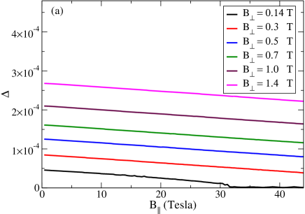
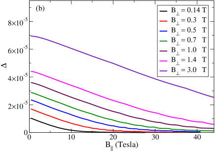
Figure 7: Gaps at the edge as a function of parallel field for a variety of perpendicular magnetic fields for armchair boundary conditions; (a) Profile B, and (b) Profile C (as defined in Fig. 5). $\Delta$ is measured in units of $E_{c}$.

We solve the self-consistent gap equation at each value of $k$ using the given order parameter and hence find $\Omega$ as a function of $k$, which allows us to determine the energies of the edge states using Eq. (6). The edge state energies for each of profiles A, B, and C introduced in Fig. 5 are illustrated in Fig. 6.

We compare the field scales for which we find a transition to ferromagnetism in Fig. 7 for profiles B and C. We find that for profile C for an armchair edge, the field scale for the gap to close is on the order of $B_{\parallel}\sim 40$ T when $B_{\perp}=0.7$ T, which is much closer to the experimental field scale of $B_{\parallel}\sim 35$ T for $B_{\perp}=1.4$ T than the uniform order parameter case, for which the gap closes for $B_{\parallel}>30$ T for $B_{\perp}=0.14$ T. Comparison between Fig. 7 (a) and (b), corresponding to order parameter spatial profiles B and C illustrates that the field scales at which the gap closes are very sensitive to the spatial variation of the order parameters near the edge. This suggests that using the theory developed in Roy et al. Roy2014 to determine the bulk order parameters and then allowing spatial variation phenomenologically is consistent with experimental results.

The agreement between the results for armchair edges and experiment is much better than the uniform case, but there are a number of factors that can be expected to be relevant at the edge that we have not included here. These include long-range Coulomb interactions, disorder, spin fluctuations and Landau level broadening Hong2019 . Nevertheless, the development of chiral symmetry breaking orders within the framework of magnetic catalysis appears to provide a consistent explanation for the experimental observations in both the bulk Roy2014 and the edge of the system for the $\nu=0$ quantum Hall state.

IV Thermal corrections

In addition to measurements of the conductance in a magnetic field at fixed temperature, in the supplementary materials of Ref. Young2014 measurements of conductance as a function of temperature were also presented. In this section we generalize the theory for self-consistent gap equations to finite temperature and then solve for the transition temperature $T_{c}$ as a function of $B$ and $\delta$ for both $\nu=0$ and $|\nu|=1$ states.

IV.1 Magnetic Catalysis at finite temperature

The zero temperature theory for the gap equations in the magnetic catalysis scenario is reviewed in Appendix B. The problem of magnetic catalysis at finite temperature has not been treated for graphene to our knowledge, but magnetic catalysis in quantum electrodynamics (QED) has been considered in the context of high energy physics Klimenko1992 ; Alexandre2001 . Finite temperature leads to additional terms in the free energy to account for entropy that lead to extra terms in the gap equations.

IV.1.1 Gap equations for $\nu=0$

To formulate the theory of magnetic catalysis at finite temperature, we note that we can write the dimensionless free energy ($f$) in the presence of antiferromagnetism and ferromagnetism as

$$f = \frac{N^{2}}{4\lambda_{a}}+\frac{M^{2}}{4\lambda_{f}}-b\left[E_{0}+\sum_{\sigma=\pm}\sum_{n=1}^{\infty}E_{n,\sigma}\right]-2bt\left[\ln\left(1+e^{-\frac{E_{0}}{t}}\right)+\sum_{\sigma=\pm}\sum_{n=1}^{\infty}\ln\left(1+e^{-\frac{E_{n,\sigma}}{t}}\right)\right],$$ (7)

$$= f_{0}-2bt\left[\ln\left(1+e^{-\frac{E_{0}}{t}}\right)+\sum_{\sigma=\pm}\sum_{n=1}^{\infty}\ln\left(1+e^{-\frac{E_{n,\sigma}}{t}}\right)\right],$$

where $f=F/hv_{F}\Lambda^{3}$, $N=N_{\perp}/(\hbar v_{F}\Lambda)$, $M=m/(\hbar v_{F}\Lambda)$, $\lambda_{a}=g_{a}\Lambda/(2\pi\hbar v_{F})$, $\lambda_{f}=g_{f}\Lambda/(2\pi\hbar v_{F})$, $t=k_{B}T/(\hbar v_{F}\Lambda)$ and $b=h\Lambda^{2}/(2B)$, with $E_{0}=\sqrt{N^{2}+M^{2}}$ and $E_{n,\sigma}=\sqrt{N^{2}+\left[\sqrt{2nb}+\sigma M\right]^{2}}$, and $f_{0}$ is the zero temperature dimensionless free energy. Minimizing the free energy gives the gap equations, which may be written in the form

$$\delta_{a}-Nyf_{1}^{a}(x,y)+\frac{N}{\sqrt{\pi}}\left[f_{2}^{a}(x,y)-yf_{3}^{a}(x)\right]+2Ny\psi_{a}(x,y,N,t) = 0,$$ (8)

$$\frac{m}{N}\delta_{f}-Nyf^{m}(x,y)+2Ny\psi_{m}(x,y,N,t) = 0,$$ (9)

where $y=B/N^{2}_{\perp}$, $x=(\lambda+m)/N_{\perp}$ and $\delta_{a}$, $\delta_{f}$, $f^{a}_{1}(x,y)$, $f^{a}_{2}(x,y)$, $f^{a}_{3}(x)$ and $f^{m}(x,y)$ are defined in Appendix B. The new functions that enter into the gap equations when thermal effects are included are

$$\psi_{a}(x,y,N,t) = \frac{1}{\sqrt{1+x^{2}}}\frac{1}{1+\exp\left[\frac{N}{t}\sqrt{1+x^{2}}\right]}+\sum_{\sigma=\pm}\sum_{n=1}^{\infty}\frac{1}{\sqrt{1+(\sqrt{2ny}+\sigma x)^{2}}}\frac{1}{1+\exp\left[\frac{N}{t}\sqrt{1+(\sqrt{2ny}+\sigma x)^{2}}\right]},$$

and

$$\psi_{m}(x,y,N,t) = \frac{x}{\sqrt{1+x^{2}}}\frac{1}{1+\exp\left[\frac{N}{t}\sqrt{1+x^{2}}\right]}+\sum_{\sigma=\pm}\sum_{n=1}^{\infty}\frac{\sigma(\sqrt{2ny}+\sigma x)}{\sqrt{1+(\sqrt{2ny}+\sigma x)^{2}}}\frac{1}{1+\exp\left[\frac{N}{t}\sqrt{1+(\sqrt{2ny}+\sigma x)^{2}}\right]}.$$

The thermal corrections to the gap equations for the in-plane antiferromagnet and the easy-axis ferromagnet are accounted for in the functions $\psi_{a}$ and $\psi_{m}$, respectively.

IV.1.2 Gap equation for $|\nu|=1$

Roy et al. Roy2014 have argued that the quantum Hall states at $|\nu|=1$ can be mainly understood as arising due to charge density wave order (another example of chiral symmetry breaking order on the honeycomb lattice HJR2009 ). Hence we can start with the dimensionless free energy ($f$) for $|\nu|=1$ states, including thermal contributions

$$f=\frac{C^{2}}{4\lambda_{c}}-b\left[\frac{E_{0}}{2}+2\sum_{n=1}^{\infty}E_{n}\right]-2bt\left[\frac{1}{2}\ln\left(1+e^{-\frac{E_{0}}{t}}\right)+2\sum_{n=1}^{\infty}\ln\left(1+e^{-\frac{E_{n}}{t}}\right)\right],$$ (12)

where $\lambda_{c}$ is a coupling constant proportional to the nearest neighbour repulsive interaction ($V_{1}$), and obtain a gap equation as before

$$\sqrt{\pi}\delta_{c}+C\int_{0}^{\infty}\frac{ds}{s^{\frac{3}{2}}}\left[1-\frac{sye^{-s}}{\tanh(sy)}+\frac{sye^{-s}}{2}\right]+\sqrt{\pi}\psi_{c}(b,C,t)=0,$$ (13)

where $y=b/C^{2}$ and

$$\psi_{c}(b,C,t)=\frac{b}{C}\frac{1}{1+e^{\frac{C}{t}}}+4b\sum_{n=1}^{\infty}\frac{1}{E_{n}}\frac{1}{1+e^{\frac{E_{n}}{t}}},$$ (14)

with $\delta_{c}=\frac{1}{4\lambda_{c}}-\frac{1}{\sqrt{\pi}}\int_{\Lambda^{-1}}^{\infty}ds/s^{\frac{3}{2}}$, and $E_{n}=\sqrt{C^{2}+2nb}$. Thermal corrections due to charge density wave order are introduced by the function $\psi_{c}$. Here $\delta_{c}$ measures the distance from the zero field critical interaction strength ($\delta_{c}=0$) for charge density wave ordering.

IV.2 Numerical Results

We solve the gap equations found in Secs. IV.1.1 and IV.1.2 numerically and present our results below for $\nu=0$ and $|\nu|=1$. All order parameters and temperatures are expressed in dimensionless units.

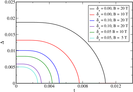
Figure 8: Gap (in units of $E_{c}$) for $\nu=0$ as a function of scaled temperature $t=k_{B}T/E_{c}$ for several different field strengths, and several different antiferromagnetic couplings $\delta_{a}$. The ferromagnetic coupling is set to $\delta_{f}=1$.

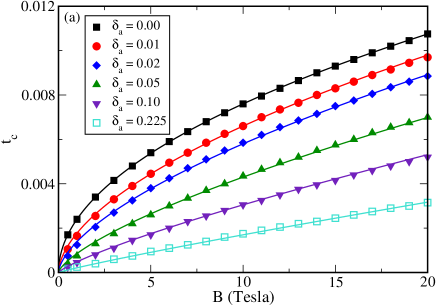
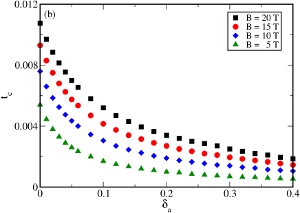
Figure 9: (a) Critical temperature $t_{c}=k_{B}T_{c}/E_{c}$ for $\nu=0$ as a function of magnetic field $B$ for six different values of $\delta_{a}$. The curves are power law fits to $t_{c}$ as a function of $B$ using Eqs. (15) and (16). (b) critical temperature $t_{c}$ for $\nu=0$ as a function of $\delta_{a}$ for four different values of magnetic field $B$. The ferromagnetic coupling is set to $\delta_{f}=1$.

IV.2.1 $\nu=0$

We solve Eqs. (8) and (9) to find the gap as a function of temperature for given $B_{\perp}$, $\delta_{a}$ with fixed $\delta_{f}=1$. We consider the situation in which the field is purely perpendicular to the graphene, so that $N_{\perp}\gg m$. We show the gap as a function of temperature for a variety of different coupling strengths and field strengths in Fig. 8. Due to the Zeeman coupling the gap $\Delta$ never goes quite to zero, even when the antiferromagnetic order parameter $N_{\perp}$ vanishes (we use this to determine the critical temperature $T_{c}$), but on the scale of Fig. 8 $N_{\perp}$ and $\Delta$ are indistinguishable. We distinguish between the dimensionful critical temperature $T_{c}$ and the dimensionless critical temperature $t_{c}=k_{B}T_{c}/E_{c}$.

The highest $t_{c}$ value shown in Fig. 8 of $t\simeq 0.011$ in scaled units corresponds to a physical temperature of $T_{c}\sim 130$ K. We extracted the critical temperature $t_{c}$ as a function of magnetic field $B$ at fixed $\delta_{a}$ and as a function of $\delta_{a}$ at fixed magnetic field $B$, as illustrated in Fig. 9. We found that we could fit the critical temperature to the following forms. For fixed $\delta_{a}$

$$t_{c}\simeq B^{\kappa},$$ (15)

with

$$\kappa\simeq\frac{1}{2}+\left(\delta_{a}\right)^{\alpha},$$ (16)

with $\alpha\sim 0.6$, and for fixed field $B$ and $\delta_{a}\lesssim 0.15$

$$t_{c}\simeq A_{B}\exp\left[-\left(\frac{\delta_{a}}{\delta_{B}}\right)^{\beta}\right],$$ (17)

where $A_{B}$ and $\delta_{B}$ are field dependent constants and $\beta\simeq 0.8$ for all fields. Recall that suspended graphene has $\delta_{a}\simeq 0.035$ and graphene on a substrate has $\delta_{a}\simeq 0.2$.

IV.2.2 $|\nu|=1$

We obtain the temperature dependence of the CDW gap for $|\nu|=1$ by solving the gap equation Eq. (13), and display the order parameter, $C$, as a function of the dimensionless temperature $t$ for various $B$ and $\delta_{c}$ in Fig. 10.

We extracted the critical temperature $t_{c}$ as a function of magnetic field $B$ at fixed $\delta_{c}$ and as a function of coupling $\delta_{c}$ at fixed magnetic field $B$, as illustrated in Fig. 11. We found that we could fit the critical temperature to similar forms that we used for $\nu=0$. For fixed $\delta_{c}$, $t_{c}$ follows Eqs. (15) and (16) with $\delta_{a}$ replaced by $\delta_{c}$ and $\alpha\sim 0.6$, and for fixed field and $\delta_{c}\lesssim 0.15$,

$$t_{c}\simeq A_{B}\exp\left[-\left(\frac{\delta_{c}}{\delta_{B}}\right)^{\beta}\right],$$ (18)

where $A_{B}$ and $\delta_{B}$ are field dependent constants and $\beta\simeq 0.75$ for all fields.

The temperature scale for $|\nu|=1$ transitions appears to be about an order of magnitude smaller than for $\nu=0$. This is consistent with the expectation that the zero temperature gap for $|\nu|=1$ is about an order of magnitude smaller than the zero temperature gap for $\nu=0$. For both states the scaling of the transition temperature $T_{c}$ with magnetic field follows closely that of the associated chiral symmetry breaking mass at zero temperature roy-scaling ; roy-inhomogeneous-catalysis . In particular, $T_{c}$ scales linearly and sublinearly for weak and subcritical interaction strengths and for critical interactions $T_{c}\sim\sqrt{B}$.

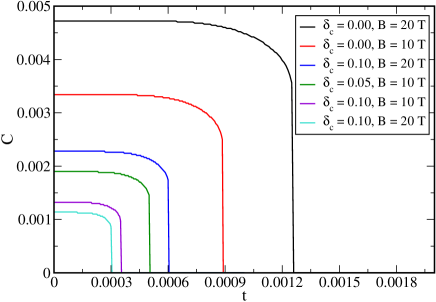
Figure 10: Gap for $|\nu|=1$ as a function of scaled temperature $t$ for several different field strengths, and several different $\delta_{c}$.

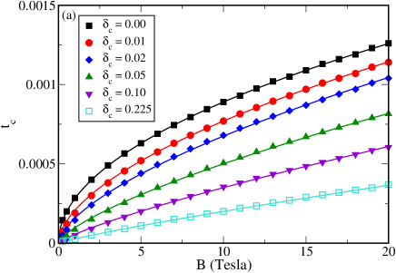
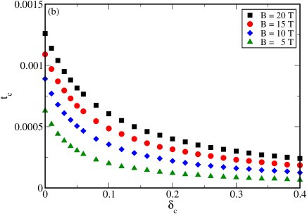
Figure 11: (a) Critical temperature $t_{c}=k_{B}T_{c}/E_{c}$ for $|\nu|=1$ as a function of magnetic field $B$ for six different values of $\delta_{c}$. The curves are power law fits to $t_{c}$ as a function of $B$. (b) critical temperature $t_{c}$ for $|\nu|=1$ as a function of $\delta_{c}$ for four different values of magnetic field $B$.

IV.3 Nature of the transition

We expect that for a single chiral symmetry breaking order parameter, the finite temperature phase transition should be second order. For $|\nu|=1$, the transition appears to be second order, with a very steep decline of the charge density wave order parameter near $T_{c}$, consistent with earlier theoretical work for the Gross-Neveu model Klimenko1992 . On the other hand, for $\nu=0$, when there is both in-plane antiferromagnetism and easy-axis ferromagnetism, as shown in Fig. 8, for $\delta_{a}$ near zero, the transition appears as though it is second order. We have noted that truncation errors in the numerical evaluation of the integrals and sums in the gap equations for $\nu=0$ (e.g. if insufficient Landau levels are included) tend to make the transition appear first order footnote .

We compared the zero temperature gap, $\Delta$, to $t_{c}$ (both in dimensionless units) for the different field and coupling strengths considered above. For $\nu=0$ we find that the relationship between $\Delta$ and $t_{c}$ is linear, and ranges from $\Delta/t_{c}=1.75$ at $\delta_{a}=0$ to $\Delta/t_{c}=2$ for $\delta_{a}=0.225$, as illustrated in Fig. 12 (a). For $|\nu|=1$ on the other hand, we find the universal scaling that $\Delta/t_{c}\approx 3.75$ for any $\delta_{c}$ as illustrated in Fig. 12 (b).

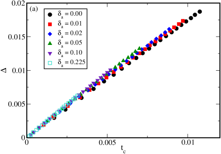
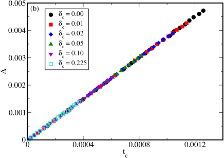
Figure 12: Zero temperature gap, $\Delta$, against critical temperature $t_{c}$ for various coupling strengths for (a) $\nu=0$ with only antiferromagnet ordering (ferromagnetism turned off) and (b) $|\nu|=1$ with charge-density-wave ordering. For $\nu=1$ we find $\Delta/t_{c}\approx 3.75$ for a wide range of interaction strengths ($\delta_{c}$).

V Discussion and Conclusions

In Ref. Roy2014 it was shown that the gaps in the bulk for the $\nu=0$ and $|\nu|=1$ quantum Hall states in monolayer graphene can be explained with a picture based on chiral symmetry breaking. While the $\nu=0$ state is compatible with a canted antiferromagnet, the $|\nu|=1$ states are likely to be due to charge density wave ordering. Both in-plane antiferromagnet and charge density wave orderings are examples of chiral symmetry breaking orders on the honeycomb lattice. In this work we explored the effects of finite sample size and finite temperature within the same scenario. We focused on edge states at $\nu=0$ and the field and interaction strength dependence of $T_{c}$ for both $\nu=0$ and $|\nu|=1$.

Experiments Young2014 have suggested that in the $\nu=0$ state there is a transition from antiferromagnetism to ferromagnetism if a strong enough parallel field is applied at fixed perpendicular field based on obervations of the increase in conductance with tilted field. This can be understood as the increasing strength of ferromagnetism decreasing the gap at the edge, and consequently allowing edge transport. Using the theory for the bulk order parameters discussed in Ref. Roy2014 we show that tilted fields have much more effect for graphene samples on a substrate than for suspended graphene. We study the edge states assuming that the order parameter at the edge is the same as in the bulk and find qualitative but not quantitative agreement with experiment in that the gap decreases with increasing tilted field, but at a much smaller perpendicular field. However, when we allow spatial variation of the order parameters near the edge with a phenomenological profile based on work in Ref. Lado2014 , the tilted field scale at which the edge gap closes is $B_{\parallel}\sim 40$ T for $B_{\perp}=0.7$ T, as illustrated in Fig. 7, which is in a similar range to experiment, emphasizing the importance of spatial variation of the order parameter near edges Jung2009 ; Tikhonov2016 ; HuangCazalilla2015 ; Murthy2016 ; Lado2014 ; Murthy2014 ; Knothe2015 .

The effect of increasing temperature on both the $\nu=0$ and $|\nu|=1$ states is to give rise to a transition to a disordered state at a non-zero critical temperature $T_{c}$ as illustrated in Figs. 8 and 10. We calculated $T_{c}$ as a function of magnetic field, $B$, and distance to the critical point, $\delta$, in Figs. 9 and 11. We found that the functional form of the dependence of $T_{c}$ on magnetic field is the same for both $\nu=0$ and $|\nu|=1$ and observe similar behaviour between the two states for the dependence of $T_{c}$ on the distance to the critical point. The magnetic field dependence of $T_{c}$ can be tested experimentally and potentially used as a way to extract $\delta_{a}$ or $\delta_{c}$ for a given sample. To study the $\delta$ dependence of $T_{c}$, using gated samples and changing the strength of screening is a way to change the distance from the critical point.

It should be noted that we have only considered the effects of short range interactions. In graphene there will also be effects from long range Coulomb interactions. These can affect the bulk behaviour and edge reconstruction and appear to be needed to obtain a full understanding of the dependence of the gap on field for $|\nu|=1$ states Roy2014 .

Our results for $\nu=0$ edge states are consistent with chiral symmetry breaking in the zeroth Landau level of monolayer graphene giving rise to the $\nu=0$ quantum Hall state. Recent consideration of fractional quantum Hall states of graphene has led to the suggestion that chiral symmetry breaking may be a unifying feature of quantum Hall states in the zeroth Landau level of monolayer graphene Narayanan2018 . Measurement of the critical temperature of the $\nu=0$ and $|\nu|=1$ integer quantum Hall states, particularly focusing on the scaling of $T_{c}$ with magnetic field would be an important additional test of this scenario and we look forward to the results of experiments investigating this behaviour.

Appendix A Calculation of edge states

In this appendix we give a brief discussion of the calculation of the edge state eigenvalues in graphene for the cases of armchair and zigzag boundary conditions (see Fig. 1). The boundary conditions arising for zigzag and armchair graphene edges are, respectively Piyatkovskiy2014 (for $H$ block diagonal in the valley index)

$$\left(I_{8}+I_{2}\otimes I_{2}\otimes\sigma_{3}\right)\Psi(y=0)=0,$$ (19)

$$\left(I_{8}+I_{2}\otimes I_{2}\otimes\sigma_{1}\right)\Psi(x=0)=0.$$ (20)

Assuming spatial uniformity of the order parameters, the eigenvalue problem can be solved analytically for the zigzag edge by utilizing the Landau gauge $\textbf{A}=(-By,0)$ and letting $\Psi(x,y)=\exp(ikx)\Psi(y)$. For armchair boundary conditions we take $\textbf{A}=(0,Bx)$ and $\Psi(x,y)=\exp(iky)\Psi(x)$.

After the valley degree of freedom has been extracted, write the spinors in the $4\times 4$ representation used for ${\mathcal{H}}$ as $\psi=\left[\psi_{1},\psi_{2},\psi_{3},\psi_{4}\right]^{T}$ and the valley spinors $\Psi_{\pm}$ can then be written as

$$\Psi_{+}=\left[\psi_{1},\psi_{2},-\psi_{4},\psi_{3}\right]^{T},$$ (21)

$$\Psi_{-}=\left[-\psi_{2},\psi_{1},\psi_{3},\psi_{4}\right]^{T}.$$ (22)

Defining $\xi=\frac{k_{x}+By}{\sqrt{B}}$, which implies $\partial_{2}=\sqrt{B}\partial_{\xi}$, we can write the eigenvalue equation ${\mathcal{H}}\psi=\varepsilon\psi$ as

$$-E_{+}\psi_{1}-\partial_{-}\psi_{2}+{\mathcal{N}}_{-}\psi_{4} = 0,$$ (23)

$$\partial_{+}\psi_{1}-E_{+}\psi_{2}+{\mathcal{N}}_{-}\psi_{3} = 0,$$ (24)

$${\mathcal{N}}_{+}\psi_{2}-E_{-}\psi_{3}-\partial_{+}\psi_{4} = 0,$$ (25)

$${\mathcal{N}}_{+}\psi_{1}+\partial_{-}\psi_{3}-E_{-}\psi_{4} = 0.$$ (26)

where we introduced $\partial_{\pm}=\partial_{\xi}\pm\xi$ and ${\mathcal{N}}_{\pm}=(N_{1}\pm iN_{2})/\sqrt{B}$ and $E_{\pm}=(\varepsilon\pm(\lambda+m))/\sqrt{B}$.

Focusing on the $\psi_{1}$ component of the spinor, we obtain the eigenvalue equation

$$\left[\partial_{-}\partial_{+}-1\right]\psi_{1}(\xi)=\Omega\psi_{1}(\xi),$$ (27)

where the eigenvalues $\Omega$ are related to the energy eigenvalues by

$$E=\pm\sqrt{{\mathcal{N}}_{\perp}^{2}+\left[(\tilde{\lambda}+\tilde{m})\pm\sqrt{-\Omega-1}\right]^{2}},$$ (28)

where ${\mathcal{N}}_{\perp}^{2}={\mathcal{N}}_{+}^{2}+{\mathcal{N}}_{-}^{2}-(N_{1}^{2}+N_{2}^{2})/B$ and $\tilde{\lambda}=\lambda/\sqrt{B}$, $\tilde{m}=m/\sqrt{B}$. Equation (27) has solutions which are parabolic cylinder functions with eigenvalue $\Omega$, which, when the solution is required to be normalizable as $y\to-\infty$ has the solutions: miransky-edge ; Piyatkovskiy2014 ; Stegun

$$\psi_{i}=g_{i}\begin{cases}U\left(\frac{1}{2}\Omega,\sqrt{2}\,\xi\right)&;i=1,4\\ U\left(\frac{1}{2}\Omega+1,\sqrt{2}\,\xi\right)&;i=2,3,\end{cases}$$

where $U(a,z)$ is the even parabolic cylinder function Stegun and the proportionality constants $g_{i}$, are defined by

$$g_{1} = 1,$$

$$g_{2} = -\frac{N_{\perp}^{2}-\left(\Omega+1\right)-\varepsilon_{-}\varepsilon_{+}}{2\sqrt{2}\left(\lambda+m\right)},$$

$$g_{3} = \frac{1}{N_{-}}\left[\varepsilon_{+}g_{2}+\frac{1}{\sqrt{2}}\left(\Omega+1\right)\right],$$

$$g_{4} = \frac{1}{N_{-}}\left[-\sqrt{2}g_{2}+\varepsilon_{+}\right],$$ (29)

where $\varepsilon_{\pm}=\varepsilon\pm(\lambda+m)$.

A.0.1 Zigzag edge

The zigzag boundary condition Eq. (19) gives the following constraints on the spinor $\Psi_{+}$

$$0 = U\left(\frac{1}{2}\Omega,\sqrt{2}\,\xi_{0}\right),$$ (30)

$$0 = \operatorname{Re}\{g_{4}\}\,U\left(\frac{1}{2}\Omega,\sqrt{2}\,\xi_{0}\right),$$ (31)

and for the spinor $\Psi_{-}$

$$0 = \operatorname{Re}\{g_{2}\}\,U\left(\frac{1}{2}\Omega+1,\sqrt{2}\,\xi_{0}\right),$$ (32)

$$0 = \operatorname{Re}\{g_{3}\}\,U\left(\frac{1}{2}\Omega+1,\sqrt{2}\,\xi_{0}\right),$$ (33)

where $\xi_{0}=k/\sqrt{B}$. Only the real part of the coefficients $g_{i}$ enter the boundary conditions since the energies $\varepsilon$, and hence the eigenvalues $\Omega$, are required to be real valued.

These boundary conditions fix the eigenvalues $\Omega=\Omega_{n\sigma s}$, where $n\in\mathbb{Z}_{\geq 0}$ labels the “branch” index and $\sigma=\pm$ labels the spin and $s=\pm$ labels the sublattice degree of freedom.

An important feature of the eigenvalue equations (30)-(33) is that they all take the form of a constant times a parabolic cylinder function, meaning that the eigenvalue determined by the vanishing of the momentum-independent coefficients $g_{i}(\Lambda)=0$, here labeled by a branch index of $n=0$, is dispersionless, while all of the higher branches (which determine the higher LLs via Eq. (4)) are determined by the vanishing of the parabolic cylinder function in question. This is in contrast to the armchair edge discussed below, where the eigenvalue is determined by a linear combination of parabolic cylinder functions, which prevents one from factoring out the zero mode edge state.

Neglecting the $n=0$ eigenvalue, the higher eigenvalues with $n\in\mathbb{N}$ then become independent of the spin index and are completely determined by the equations

$$0=U\left(\frac{1}{2}\Omega,\sqrt{2}\,\xi_{0}\right),$$ (34)

and

$$0=U\left(\frac{1}{2}\Omega+1,\sqrt{2}\,\xi_{0}\right),$$ (35)

in the $+$ and $-$ valleys, respectively. The roots $\Omega_{ns}$ of these equations are all negative definite as a function of $\xi_{0}$ Stegun . If one takes the bulk limit, which corresponds to $\xi\rightarrow\infty$, then the eigenvalues $\Omega\rightarrow-2n-1$ where $n\in\mathbb{Z}_{\geq 0}$ Stegun ; Piyatkovskiy2014 , and the expression for the energy eigenvalues, Eq. (4), reduces to

$$E=\pm\sqrt{{\mathcal{N}}_{\perp}^{2}+\left[(\tilde{\lambda}+\tilde{m})\pm\sqrt{2n}\right]^{2}},$$ (36)

in agreement with the expected expression Roy2014 .

A.0.2 Armchair edge

The armchair boundary condition Eq. (20) imposes the pair of constraints

$$0 = U\left(\frac{1}{2}\Omega,\sqrt{2}\,\xi_{0}\right)+s^{\prime}\operatorname{Re}\{g_{2}\}\,U\left(\frac{1}{2}\Omega+1,\sqrt{2}\,\xi_{0}\right),$$

$$0 = \operatorname{Re}\{g_{3}\}\,U\left(\frac{1}{2}\Omega+1,\sqrt{2}\,\xi_{0}\right)$$ (38)

$$-s^{\prime}\operatorname{Re}\{g_{4}\}\,U\left(\frac{1}{2}\Omega,\sqrt{2}\,\xi_{0}\right),$$

on the $s^{\prime}=\pm$ valley. We solve Eqs. (LABEL:eq:armchairbc1) and (38) numerically to obtain $\Omega$, and hence, using Eq. (28), the energy spectrum of the edge modes, which are displayed in Secs. II.2 and III.

Appendix B Zero temperature gap equations

The gap equations that we use for the bulk have been discussed in considerable detail elsewhere herbut2007 ; roy-BLG ; Roy2014 . We give a brief summary of their derivation here for $\nu=0$ in order to facilitate our discussion of magnetic catalysis at finite temperature in Sec. IV. In the bulk, when there are both AFM and FM orders the LLs have the form $\pm E_{n,\sigma}$, where herbut2007

$$E_{n,\sigma}=\sqrt{N^{2}_{\perp}+[(N^{2}_{3}+2nB)^{1/2}+\sigma(m+\lambda)]^{2}},$$ (39)

with $N_{3}$ and $N_{\perp}$ the easy-axis and easy-plane components of the Neel order parameter respectively and $\sigma=\pm$ the two spin projections. The degeneracy of the LLs is $D=1/(\pi l^{2}_{B})$ for $n\geq 1$ and $1/(2\pi l^{2}_{B})$ for $n=0$ Roy2014 . The corresponding zero temperature free energy herbut2007 ; roy-BLG ; Roy2014 is obtained from a sum over filled LLs (for $n\geq 1$):

$$F_{0}=\frac{N^{2}_{\perp}+N^{2}_{3}}{4g_{a}}+\frac{m^{2}}{4g_{f}}-D\sum_{\sigma=\pm}\left[\frac{1}{2}E_{0,\sigma}+\sum_{n\geq 1}E_{n,\sigma}\right],$$

where $g_{a}$ ($g_{f}$) are couplings arising from short-range interactions, such as on-site Hubbard repulsion, that support AFM (FM) order comment-1 ; Roy2014 . For non-trivial Zeeman coupling ($\lambda\neq 0$), $F_{0}$ is minimized when $N_{3}\equiv 0$ herbut2007 ; roy-BLG . Therefore, the Zeeman coupling restricts the AFM order to the easy-plane and simultaneously allows FM order parallel to the magnetic field. Taking $N_{3}=0$ and then minimizing $F_{0}$ with respect to $N_{\perp}$ and $m$ leads to coupled gap equations Roy2014 . Ferromagnetic order splits all the filled LLs, including the zeroth one, while easy plane AFM order lowers the energy of all of the filled LLs in addition to splitting the ZLL. Hence the contribution from the filled LLs with $n\geq 1$ in the first (second) gap equation add up (cancel). Consequently, the second gap equation is free of divergences, but the first one exhibits an ultraviolet divergence which can be regularized as discussed in Refs. herbut-qhe ; roy-scaling ; Roy2014 and written in terms of $\delta_{a}=\frac{1}{4\lambda_{a}}-\frac{1}{\sqrt{\pi}}\int_{\Lambda^{-1}}^{\infty}ds/s^{\frac{3}{2}}$ where $(\lambda^{a}_{c})^{-1}=\int^{\infty}_{\Lambda^{-1}}ds/s^{3/2}$ is the zero magnetic field critical onsite interaction strength for AFM ordering HerbutPRL2006 ; HJR2009 ; herbut-assaad2013 and $\delta_{f}=1/2\lambda_{f}$. The relation between $\lambda_{a,f}$ and $g_{a,f}$ was specified in Sec. IV.1.1. Thus the two gap equations, after regularization, can be written compactly as

$$\delta_{a}-N_{\perp}yf^{a}_{1}(x,y)+\frac{N_{\perp}}{\sqrt{\pi}}\left(f_{2}^{a}(x,y)-yf_{3}^{a}(x)\right) = 0,$$ (41)

$$\frac{m}{N_{\perp}}\delta_{f}-N_{\perp}yf^{m}(x,y) = 0,$$ (42)

where we have introduced $y=B/N^{2}_{\perp}$ and $x=(\lambda+m)/N_{\perp}$. The various functions appearing in these two equations are given by

$$f^{a}_{1}(x,y) = \sum_{n\geq 0}\sum_{\sigma=\pm}\left[\frac{1}{\left[1+\left(\sqrt{2ny}+\sigma x\right)^{2}\right]^{1/2}}-\frac{1}{\left(1+2ny\right)^{1/2}}\right],$$ (43)

$$f^{a}_{2}(x,y) = \int^{\infty}_{0}\frac{ds}{s^{3/2}}\left[1-sye^{-s}\coth(sy)\right],$$ (44)

$$f^{a}_{3}(x,y) = \int^{\infty}_{0}\frac{ds}{s^{1/2}}e^{-s}\left(1-e^{-sx^{2}}\right),$$ (45)

$$f^{m}(x,y) = \left[\sum_{n\geq 0}\sum_{\sigma=\pm}\frac{\sigma\left(\sqrt{2ny}+\sigma x\right)}{\left[1+\left(\sqrt{2ny}+\sigma x\right)^{2}\right]^{1/2}}\right]-\frac{x}{(1+x^{2})^{1/2}}.$$ (46)

References

- (1) K. S. Novoselov, A. K. Geim, S. V. Morozov, D. Jiang, M. I. Katsnelson, I. V. Grigorieva, S. V. Dubonos, and A. A. Firsov, Nature (London) 438, 197 (2005).
- (2) Y. Zhang, Y.-W. Tan, H. L. Stormer, and P. Kim, Nature (London) 438, 201 (2005).
- (3) V. P. Gusynin, and S. G. Sharapov, Phys. Rev. Lett. 95, 146801 (2005).
- (4) Y. Zhang, Z. Jiang, J. P. Small, M. S. Purewal, Y.-W. Tan, M. Fazlollahi, J. D. Chudow, J. A. Jaszczak, H. L. Stormer, and P. Kim, Phys. Rev. Lett. 96, 136806 (2006).
- (5) I. Skachko, X. Du, F. Duerr, A. Luican, D. A. Abanin, L. S. Levitov, E.Y. Andrei, Phil. Trans. R. Soc. A 368, 5403 (2010).
- (6) D. A. Abanin, B. E. Feldman, A. Yacoby, and B. I. Halperin, Phys. Rev. B 88, 115407 (2013).
- (7) G. L. Yu, R. Jalil, B. Belle, A. S. Mayorov, P. Blake, F. Schedin, S. V. Morozov, L. A. Ponomarenko, F. Chiappini, S. Wiedmann, U. Zeitler, M. I. Katsnelson, A. K. Geim, K. S. Novoselov, and D. C. Elias, Proc. Nat. Acad. Sci. 110, 3282 (2013).
- (8) A. F. Young, C. R. Dean, L. Wang, H. Ren, P. Cadden-Zimansky, K. Watanabe, T. Taniguchi, J. Hone, K. L. Shepard, and P. Kim, Nat. Phys. 8, 550 (2012).
- (9) X. Du, I. Bkachko, F. Duerr, A. Luican, E. Y. Andrei, Nature 462, 192 (2009).
- (10) C. R. Dean, A. F. Young, P. Cadden-Zimansky, L. Wang, H. Ren, K. Watanabe, T. Taniguchi, P. Kim, J. Hone, and K. L. Shepard, Nat. Phys. 7, 693 (2011).
- (11) B. E. Feldman, B. Krauss, J. H. Smet, A. Yacoby, Science 337, 1196 (2012).
- (12) S.-Y. Li, Y. Zhang, L. J. Yin, and L. He, Phys. Rev. B 100, 085437 (2019).
- (13) S. J. Hong, C. Belke, J. C. Rode, B. Brechtken, and R. J. Haug, electronic preprint arXiv:1908.02420v1.
- (14) B. Roy, M. P. Kennett, and S. Das Sarma, Phys. Rev. B 90, 201409(R) (2014).
- (15) D. V. Khveshchenko, Phys. Rev. Lett. 87, 246802 (2001); H. Leal and D. V. Khveshchenko, Nucl. Phys. B687, 323 (2004).
- (16) I. F. Herbut, Phys. Rev. Lett. 97, 146401 (2006).
- (17) I. F. Herbut, V. Juričić, and B. Roy, Phys. Rev. B 79, 085116 (2009).
- (18) I. F. Herbut, Phys. Rev. B 75, 165411 (2007).
- (19) I. F. Herbut, Phys. Rev. B 76, 085432 (2007).
- (20) K. Yang, Solid State Commun. 143, 27 (2007).
- (21) G. W. Semenoff and F. Zhou, JHEP 1107, 037 (2011).
- (22) M. O. Goerbig, Rev. Mod. Phys. 83, 1193 (2011).
- (23) Y. Barlas, K. Yang, and A. H. MacDonald, Nanotechnology 23, 052001 (2012).
- (24) M. Kharitonov, Phys. Rev. B 85, 155439 (2012).
- (25) S. Narayanan, B. Roy, and M. P. Kennett, Phys. Rev. B 98, 235411 (2018).
- (26) V. P. Gusynin, V. A. Miransky, and I. A. Shovkovy, Phys. Rev. Lett. 73, 3499 (1994).
- (27) E. V. Gorbar, V. P. Gusynin, V. A. Miransky, I. A. Shovkovy, Phys. Rev. B 66, 045108 (2002).
- (28) I. F. Herbut and B. Roy, Phys. Rev. B 77, 245438 (2008).
- (29) B. Roy and I. F. Herbut, Phys. Rev. B 83, 195422 (2011).
- (30) I. A. Shovkovy, Magnetic Catalysis: A Review. In: Kharzeev D., Landsteiner K., Schmitt A., Yee HU. (eds) Strongly Interacting Matter in Magnetic Fields. Lecture Notes in Physics, vol 871. Springer, Berlin, Heidelberg (2013).
- (31) Y. Tada, Phys. Rev. Research 2, 033363 (2020).
- (32) K. Yang, S. Das Sarma, and A. H. MacDonald, Phys. Rev. B 74, 075423 (2006).
- (33) M. O. Goerbig, R. Moessner, and B. Doucot, Phys. Rev. B 74, 161407(R) (2006).
- (34) J.-N. Fuchs and P. Lederer, Phys. Rev. Lett. 98, 016803 (2007).
- (35) K. Nomura and A. H. MacDonald, Phys. Rev. Lett. 96, 256602 (2006).
- (36) J. Jung and A. H. MacDonald, Phys. Rev. B 80, 235417 (2009).
- (37) V. P. Gusynin, V. A. Miransky, S. G. Sharapov, and I. A. Shovkovy, Phys. Rev. B 74, 195429 (2006).
- (38) B. Feshami and H. A. Fertig, Phys. Rev. B 94, 245435 (2016).
- (39) V. Lukose and R. Shankar, Phys. Rev. B 94, 085135 (2016).
- (40) T. O. Wehling, E. Sasioglu, C. Friedrich, A. I. Lichtenstein, M. I. Katsnelson, and S. Blügel, Phys. Rev. Lett. 106, 236805 (2011).
- (41) D. A. Abanin, K. S. Novoselov, U. Zeitler, P. A. Lee, A. K. Geim, and L. S. Levitov, Phys. Rev. Lett. 98, 196806 (2007).
- (42) H. A. Fertig and L. Brey, Phys. Rev. Lett. 97, 116805 (2006).
- (43) A. F. Young, J. D. Sanchez-Yamagishi, B. Hunt, S. H. Choi, K. Watanabe, T. Taniguchi, R. C. Ashoori, and P. Jarillo-Herrero, Nature 505, 528 (2014).
- (44) P. K. Pyatkovskiy, and V. A. Miransky, Phys. Rev. B 90, 195407 (2014).
- (45) P. Tikhonov, E. Shimshoni, H. A. Fertig, and G. Murthy, Phys. Rev. B 93, 115137 (2016).
- (46) C. Huang and M. A. Cazalilla, Phys. Rev. B 92, 155124 (2015).
- (47) G. Murthy, E. Shimshoni, and H. A. Fertig, Phys. Rev. B 93, 045105 (2016).
- (48) J. L. Lado and J. Fernández-Rossier, Phys. Rev. B 90, 165429 (2014).
- (49) G. Murthy, E. Shimshoni, and H. A. Fertig, Phys. Rev. B 90, 241410(R) (2014).
- (50) A. Knothe and T. Jolicoeur, Phys. Rev. B 92, 165110 (2015).
- (51) V. P. Gusynin, V. A. Miransky, S. G. Sharapov, and I. A. Shovkovy, Phys. Rev. B 77, 205409 (2008).
- (52) V. P. Gusynin, V. A. Miransky, S. G. Sharapov, I. A. Shovkovy, and C. M. Wyenberg, Phys. Rev. B 79, 115431 (2009).
- (53) In Ref. Roy2014 , the coupling is reported as 0.05. The correct value of for the fits in Ref. Roy2014 is .
- (54) K. G. Klimenko, Z. Phys. C 54, 323 (1992).
- (55) J. Alexandre, K. Farakos, and G. Koutsoumbas, Phys. Rev. D 63, 065015 (2001).
-
(56)
If the transition is first order, then this is likely a consequence of the coupling to the non-zero
ferromagnetic order. The possibility of a first order transition when one has two coupled order parameters can be seen from
the Landau free energy
where is the ferromagnetic order parameter and the in-plane antiferromagnetic order parameter, which is a minimal free energy for the state. Here, are unknown coeffcients, and can be identified with external magnetic field. The equilibrium value of is non-zero, and when substituted into gives a free energy of the form
with . If , then terms are required to stabilize the free energy and a first order phase transition results. - (57) M. Abramowitz, and I. A. Stegun, Handbook of Mathematical Functions with Formulas, Graphs, and Mathematical Tables, U.S. Gov. Printing Office, Washiington, D.C. (1972).
- (58) See B. Roy, Phys. Rev. B 89, 201401(R) (2014) for discussion on easy-plane layer AFM in bilayer graphene.
- (59) Although both and arise from onsite repulsion (), in the presence of magnetic fields herbut2007 ; roy-BLG .
- (60) F. F. Assaad and I. F. Herbut, Phys. Rev. X 3, 031010 (2013).