Reinforcement learning and Bayesian data assimilation for model-informed precision dosing in oncology

Abstract

Model-informed precision dosing (MIPD) using therapeutic drug/biomarker monitoring offers the opportunity to significantly improve the efficacy and safety of drug therapies. Current strategies comprise model-informed dosing tables or are based on maximum a-posteriori estimates. These approaches, however, lack a quantification of uncertainty and/or consider only part of the available patient-specific information. We propose three novel approaches for MIPD employing Bayesian data assimilation (DA) and/or reinforcement learning (RL) to control neutropenia, the major dose-limiting side effect in anticancer chemotherapy. These approaches have the potential to substantially reduce the incidence of life-threatening grade 4 and subtherapeutic grade 0 neutropenia compared to existing approaches. We further show that RL allows to gain further insights by identifying patient factors that drive dose decisions. Due to its flexibility, the proposed combined DA-RL approach can easily be extended to integrate multiple endpoints or patient-reported outcomes, thereby promising important benefits for future personalized therapies.

¹Institute of Mathematics, University of Potsdam, Germany
²Graduate Research Training Program PharMetrX: Pharmacometrics & Computational Disease Modelling, Freie Universität Berlin and University of Potsdam, Germany
³Department of Clinical Pharmacy and Biochemistry, Institute of Pharmacy, Freie Universität Berlin, Germany
^∗ corresponding author
^† these authors contributed equally to this work
Institute of Mathematics, Universität Potsdam
Karl-Liebknecht-Str. 24-25, 14476 Potsdam/Golm, Germany
Tel.: +49-977-59 33, Email: huisinga@uni-potsdam.de, wiljes@uni-potsdam.de

Conflict of Interest/Disclosure

CK and WH report research grants from an industry consortium (AbbVie Deutschland GmbH & Co. KG, AstraZeneca, Boehringer Ingelheim Pharma GmbH & Co. KG, Grünenthal GmbH, F. Hoffmann-La Roche Ltd., Merck KGaA and Sanofi) for the PharMetrX program. In addition CK reports research grants from the Innovative Medicines Initiative-Joint Undertaking (‘DDMoRe’), from H2020-EU.3.1.3 (’FAIR’) and Diurnal Ltd. All other authors declare no competing interests for this work.

Funding information

• Graduate Research Training Program PharMetrX: Pharmacometrics & Computational Disease Modelling, Berlin/Potsdam, Germany,

• Deutsche Forschungsgemeinschaft (DFG) - SFB1294/1 - 318763901 (associated project).

• Deutsche Forschungsgemeinschaft and Open Access Publishing Fund of University of Potsdam.

Keywords

Data assimilation, Oncology, Chemotherapy, Therapeutic Drug Monitoring, Model-Informed Precision Dosing

1 INTRODUCTION

Personalized dosing offers the opportunity to improve safety and efficacy of drugs beyond the current practice [1]. This is particularly crucial for drugs that exhibit narrow therapeutic indices relative to the variability between patients. Patient-specific dose adaptations during ongoing treatments are, however, difficult due to the need to integrate multiple sources of information, the lack of precise guidelines for dose adaptations in the label and limited time resources [2, 3].

A particularly critical case is cytotoxic anticancer chemotherapy with neutropenia as major dose-limiting toxicity [4]. Patients with severe neutropenia experience a drastic reduction of neutrophil granulocytes and are thus highly susceptible to potentially life-threatening infections. Depending on the lowest neutrophil concentration (nadir), the different grades $g$ of neutropenia range from no neutropenia ($g=0$) to life-threatening ($g=4$) [5]. At the same time, neutropenia serves as a surrogate for efficacy (in terms of median survival) [6, 7, 8]. Neutrophil counts can therefore be used as a biomarker to guide dosing [9, 10, 11].

In this article, we consider paclitaxel-induced neutropenia as an illustrative and therapeutically relevant application. Paclitaxel is used as first-line treatment against non-small-cell lung cancer in platinum-based combination therapy [12]. The standard dosing of paclitaxel is based on the patient’s body surface area (BSA). To individualize treatment, a dosing table based on sex, age, BSA, drug exposure and toxicity was developed [13] and evaluated in a clinical trial (hereafter “CEPAC-TDM study”) [14].

Model-informed precision dosing (MIPD) describes approaches for dose individualization that take into account prior knowledge on the drug-disease-patient system and associated variability, e.g., from a nonlinear mixed effects (NLME) analysis as well as patient-specific therapeutic drug/biomarker monitoring (TDM) data [15]. A popular approach is based on maximum a-posteriori (MAP) estimation [16, 17, 18], which infers the individual model parameters of the pharmacokinetic/pharmacodynamic (PK/PD) model. MAP-based outcomes are typically evaluated with respect to a utility function or a target concentration to determine the next dose (MAP-guided dosing) [19, 17]. The definition of a target concentration or utility function is, however, difficult since in many therapies rather subtherapeutic or toxic ranges are known. For therapeutic ranges MAP-guided dosing is inaccurate [20], since only a point estimate is used, neglecting associated uncertainties [21].

Recently, we have shown that Bayesian data assimilation (DA) approaches provide more informative clinical decision support, fully exploiting patient-specific information [21]. DA allows for individualized uncertainty quantification, which is a necessity (i) to integrate both, safety and efficacy aspects into the objective function of finding the optimal dose, or (ii) to compute the probability of being within/outside the target range. However, optimizing across a whole therapy time frame can be hard and potentially too costly for real-time decision support.

Reinforcement learning (RL) has been applied to various fields in health care, however, mainly focusing on clinical trial design [22, 23], and only few studies relate to optimal dosing in a PK/PD context [24, 25]. In model-based RL, it is learned how to act best in an uncertain environment using model simulations. A key aspect of learning is to make successively use of knowledge already acquired, while also exploring yet unknown sequences of actions. The result is typically a decision tree (or some functional relationship). In other words, the physician’s decision is supported via a pre-calculated, extensive and detailed look-up table without additional online computation. So far, RL approaches in health care are limited to rather simple exploration strategies (so-called $\epsilon$-greedy approaches) with one time step ahead approximations of the look-up table (Q-learning) [23].

In this article, we demonstrate how DA and RL can be very beneficially exploited to develop new approaches to MIPD. The first approach, referred to as DA-guided dosing, improves existing online MIPD by integrating model uncertainties into the dose selection process. For the second approach (RL-guided dosing) we propose Monte Carlo tree search (MCTS) in conjunction with the upper confidence bound applied to trees (UCT) [26, 27] as sophisticated learning strategy. The third approach combines DA and RL (DA-RL-guided) to make full use of patient TDM data and to provide a flexible, interpretable and extendable framework. We compared the three proposed approaches with current dosing strategies in terms of dosing performance and their ability to provide insights into the factors driving dose selection.

2 METHODS

We consider a single dose every three weeks schedule for paclitaxel-based chemotherapy, usually termed a cycle $c=1,\dots,C$, for a total of six cycles ($C=6$). We denote the decision time point for the dose of cycle $c$ by $T_{c}$, and assume $T_{1}=0$ (therapy start). For dose selection, the physician has different sources of information available, such as the patient’s covariates ‘cov’ (sex, age, etc), the treatment history (drug, dosing regimen, etc), TDM data related to PK/PD (drug concentrations, response, toxicity, etc). Despite these multiple sources of information, it remains a partial and imperfect information problem, as only noisy measurements of few quantities of interest at certain time points are available. MIPD aims to provide decision support by linking prior information on the drug-patient-disease system with patient-specific TDM data.

The standard dosing for 3-weekly paclitaxel, as applied in the CEPAC-TDM study arm A, is $200\,\text{mg}/\text{m}^{2}\,\text{BSA}$ and a 20 % dose reduction if neutropenia grade 4 ($g_{c}=4$) was observed [14]. The aforementioned dosing table (termed PK-guided dosing [13]) was evaluated in study arm B, see Section S 3. For dose selection at cycle start $T_{c}$, we chose the patient state

$$s_{c-1}=\Big{(}\text{sex},\text{age};\;\text{ANC}_{0},g_{1},\ldots,g_{c-1}\Big{)}\,,$$ (1)

with $s_{0}=(\text{sex},\text{age};\;\text{ANC}_{0})$. The covariates sex, age, have previously been identified as important predictors of exposure [13], and baseline absolute neutrophil counts $\text{ANC}_{0}$, as a crucial parameter in the drug-effect model [28, 29]. We included the neutropenia grades of all previous cycles $g_{1:c-1}=(g_{1},\ldots,g_{c-1})$ to account for the observed cumulative behavior of neutropenia [29, 30].

2.1 MIPD framework

MIPD builds on prior knowledge from NLME analyses of clinical studies [21]. The structural and observational models are generally given as

$$\frac{\mathrm{d}x}{\mathrm{d}t}(t) =f(x(t);\theta,d),\qquad x(0)=x_{0}(\theta)$$ (2)

$$h(t) =h(x(t),\theta)$$ (3)

with state vector $x=x(t)$ (e.g., neutrophil concentration), parameter values $\theta$ (e.g., mean transition time) and rates of change $f(x;\theta,d)$ for given doses $d$. The initial conditions $x_{0}$ are given by the pre-treatment levels (e.g., $\text{ANC}_{0}$). A statistical model links the observables, the quantities that can be measured $h_{j}(\theta)=h(x(t_{j}),\theta)$ at time points $t_{j}$ to observations $(t_{j},y_{j})_{j=1,\ldots,n}$ taking into account measurement errors and potential model misspecifications, e.g.,

$$Y_{j|\Theta=\theta}=h_{j}(\theta)+\epsilon_{j}\,$$ (4)

with $\epsilon_{j}\sim_{\mathrm{iid}}\mathcal{N}(0,\Sigma)$. In more general terms, $Y_{j|\Theta=\theta}\sim p\big{(}\,\cdot\,|\theta;h_{j}(\theta),\Sigma\big{)}\,,$ with $j=1,\dots,n$ independent. The prior distribution for the individual parameters is given by a covariate and statistical model,

$$\Theta\sim p_{\Theta}\big{(}\theta^{\textrm{TV}}(\text{cov}),\Omega\big{)}$$ (5)

with $\theta^{\textrm{TV}}(\text{cov})$ denoting the typical values (TV), which generally depend on covariates ‘cov’, and $\Omega$ the inter-individual variability . We used the term ‘model’ to refer to eqs. (2)-(5), and the term ‘model state of the patient’ to refer to a model-based representation of the state of the patient, i.e., a distribution of state-parameter pairs $(x,\theta)$, or just a single (reference) state-parameter pair. In the proposed approaches, the model is used to simulate treatment outcomes (in RL called “simulated experience”), or to assimilate TDM data and infer the model state of the patient, or both. To infer the patient state (1), the grade of neutropenia of the previous cycle $g_{c-1}$ needs to be determined; either directly from the TDM data ($y_{c-1}\mapsto g_{c-1}\mapsto s_{c-1}$) or based on a model simulation of the model state of the patient ($(x,\theta)\mapsto c_{\text{nadir}}\mapsto g_{c-1}\mapsto s_{c-1}$).

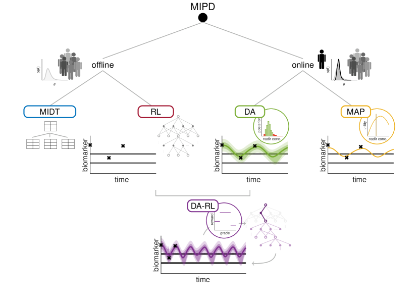
Figure 1: Overview of different approaches for model-informed precision dosing (MIPD). The different methods can be categorized according to the time when the computational effort to calculate the optimal dose must be made. Offline approaches calculate optimal doses for all possible covariates and state combinations prior to any treatment, like in model-informed dosing tables (MIDT) and reinforcement learning (RL). The physician selects the dosing recommendation in the table/tree based on specific patient information (covariates, observations). While the TDM data (measured biomarker) are used to determine the entry in the table/tree, the table/tree itself is static. Online approaches solve an optimization problem at any decision time point, i.e., when a dose has to be given. They integrate patient-specific TDM data using Bayesian data assimilation (DA) or maximum a-posteriori (MAP) estimation. Offline–online approaches allocate computational resources between offline and online. Pre-calculated dosing decision-trees are individualized during treatment, based on TDM data.

We considered three different approaches towards MIPD, see Figure 1:

(i) Offline approaches support dose individualization based on model-informed dosing tables (MIDT) or dosing decision trees (RL-guided dosing). At the start of therapy a dose based on the patient’s covariates and baseline measurements is recommended. During therapy, the observed TDM data are used to determine a path through the table/tree; While the treatment is individualized to the patient (based on a-priori uncertainties), the procedure of dose individualization itself does not change, i.e., the tree/table is static. As such, it can be communicated to the physician before the start of therapy.

(ii) Online approaches determine dose recommendations based on a model state of the patient and its simulated outcome. Bayesian DA or MAP estimation assimilate individual TDM data to infer the posterior distribution or MAP point-estimate as model state of the patient, respectively. While online approaches tailor the model (more precisely, the parameters) to the patient, clinical implementation requires an IT infrastructure and expert personnel, which constitutes a current challenging problem and hinders broad application [31].

(iii) Offline–Online approaches combine the advantages of dosing decision trees and an individualised model. The individualised model is used in two ways, to infer the patient state more reliably than sparsely observed TDM data and to individualize the dosing decision tree (using individualized uncertainties, rather than population-based uncertainties).

Key to all approaches is the so-called reward function $R$ (RL terminology), also termed cost or utility function, defined on the set $\mathcal{S}$ of patient states

$$R:\mathcal{S}\rightarrow\mathbb{R}.$$ (6)

Ideally, the reward corresponds to the net utility of beneficial and noxious effects in a patient given the current state [32]. For neutrophil-guided dosing, a reward function was suggested that maps (MAP-based) nadir concentrations to a continuous score [19] or penalizes the deviation from a target nadir concentration [17], see also Section S 8.5 and Figure S 8. The individualized uncertainties quantified via DA allow to consider the probability of being within/outside the target range in the reward function [21], which is more closely related to clinical reality. For the patient state (1) used in RL we also designed the reward function to account for efficacy and toxicity. We chose to penalize the short-term goal (avoiding life-threatening grade 4) more than the long-term goal (increased median survival associated with neutropenia grades 1-4 [8]) :

$$R(s_{c})=\begin{cases}-1\qquad\text{if $g_{c}=0$}\,,\\ \hphantom{-}1\qquad\text{if $g_{c}=1,2,3$}\,,\\ -2\qquad\text{if $g_{c}=4$}\,.\end{cases}$$ (7)

2.2 RL-guided dosing

RL problems can be formalized as Markov decision processes, modeling sequential decision making under uncertainty, and are closely related to stochastic optimal control [33]. In RL, the goal of a so-called agent (here: the virtual physician) is to learn a policy (strategy) of how to act (dose) best with respect to optimizing a specific expected long-term return (response), given an uncertain and delayed feedback environment (virtual patient) [34, 35, 36, 37], see Figure 2.

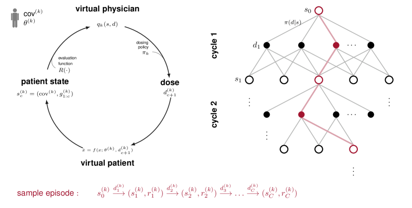
Figure 2: Model-based reinforcement learning (planning). The expected long-term return (action-value function) is estimated based on simulated experience (sample approximation Eq. (12)). For simulating experience, an ensemble of virtual patients is generated, $k=1\dots,K$ (for all covariate classes $\mathcal{COV}_{l}$, $l=1,\dots,L$, covariates cov^(k) are sampled within the covariate class and model parameters $\theta^{(k)}$ are sampled from the prior distribution). At start of each cycle $c$, a dose $d_{c+1}^{(k)}$ is chosen according to the current policy $\pi_{k}$, and the outcome (grade of neutropenia) is predicted based on the model $\dot{x}=f(x;\theta^{(k)},d_{c}^{(k)})$ for the sample parameter vector $\theta^{(k)}$ and chosen dose. The updated patient state $s_{c}^{(k)}$ is assessed using the reward function $R$. The sequential dose selections (going through the circle $C$ times (left part)) lead to so-called sample episodes; the entirety of episodes to a tree structure.

A Markov decision process comprises a sequence including states $S_{c}$, actions $D_{c}$ and rewards $R_{c}$ with the subscript $c$ referring to time (e.g., treatment cycle). If there is a natural notion of a final time $c=C$ (e.g., therapy of six cycles), the sequence is called an episode. Every episode corresponds to a path in the tree of possibilities (Figure 2). Due to unexplained variability between patients (and occasions), transitions between states are characterized by transition probabilities $\mathbb{P}[S_{c+1}=s_{c+1}|S_{c}=s_{c},D_{c+1}=d_{c+1}]$. The reward is defined via the reward function, i.e., $R_{c}=R(S_{c})$, while a so-called dosing policy $\pi$ models how to choose the next dose

$$\pi(d|s)=\mathbb{P}[D_{c+1}=d|S_{c}=s].$$ (8)

A dosing policy is evaluated based on the so-called return $G_{c}$ at time step $c$, defined as the weighted sum of rewards over the remaining course of therapy

$$G_{c}=R_{c+1}+\gamma R_{c+2}+\dots+\gamma^{C-(c+1)}R_{C}=\sum_{k=c+1}^{C}\gamma^{k-(c+1)}R_{k}\,.$$ (9)

The discount factor $\gamma\in[0,1]$ balances between short-term ($\gamma\rightarrow 0$) and long-term ($\gamma\rightarrow 1$) therapeutic goals (see Sections S 6 and S 8.7.1). Ultimately, the objective is to maximize the expected long-term return

$$q_{\pi}(s,d):=\mathbb{E}_{\pi}[G_{c}|S_{c}=s,D_{c+1}=d]\,,$$ (10)

given the current state $S_{c}=s$ and dose $D_{c+1}=d$ over the space of dosing policies $\pi$. The function $q_{\pi}$ is called the action-value function [35]. Due to the close interplay between $q_{\pi}$ and $\pi$, learning an optimal policy involves an iterative process of value estimation and policy improvement [35].

Model-based RL methods that rely on sampling (sample-based planning) estimate the expected value in eq. (10) via a sample approximation. To simplify the calculations we have discretized ‘age’ and ANC₀ into covariate classes $\mathcal{COV}_{l}$, $l=1,\dots,L$. For each class $\mathcal{COV}_{l}$ consider the ensemble

$$\mathcal{E}_{\text{RL}}(\mathcal{COV}_{l}):=\Big{\{}\big{(}x_{0}(\theta_{c}^{(k)}),\theta_{c}^{(k)},\text{cov}^{(k)}\big{)}\Big{\}}_{k=1}^{K}$$

with $\text{cov}^{(k)}$ sampled within $\mathcal{COV}_{l}$ according to the covariate distributions in the CEPAC-TDM study [14, 38], parameter values sampled from $p_{\Theta}\big{(}\theta^{\textrm{TV}}(\text{cov}^{(k)}),\Omega\big{)}$ and initial states according to (2). Then, for each $k=1,\ldots,K$ with $K$ large, a sample episode

$$s_{0}^{(k)}\overset{d_{1}^{(k)}}{\longrightarrow}(s_{1}^{(k)},r_{1}^{(k)})\overset{d^{(k)}_{2}}{\longrightarrow}(s^{(k)}_{2},r^{(k)}_{2})\overset{d^{(k)}_{3}}{\longrightarrow}\ldots\overset{d^{(k)}_{C}}{\longrightarrow}(s^{(k)}_{C},r^{(k)}_{C})$$ (11)

using policy $\pi_{k}$ is determined and

$$q_{k}(s,d)=\frac{1}{N_{k}(s,d)}\sum_{k^{\prime}=1}^{k}\sum_{c=1}^{n_{c}}\mathbbm{1}_{(s_{c}^{(k^{\prime})}=s,d^{(k^{\prime})}_{c+1}=d)}G_{c}^{(k^{\prime})}$$ (12)

computed. Here, $N_{k}(s,d)$ denotes the number of times that dose $d$ was chosen in patient state $s$ amongst the first $k$ episodes, and $G_{c}^{(k)}=r^{(k)}_{c+1}+\gamma r^{(k)}_{c+2}+\ldots$. Ideally, $N_{k}(s,d)$ should be large for each state-dose combination to guarantee a good approximation of the expected return (law of large numbers). This, however, is infeasible for most applications (curse of dimensionality).

Therefore, we employed MCTS in conjunction with UCT as policy in the iterative training process [39, 40, 26, 41, 27]:

$$\pi_{k+1}(d_{c+1}|s_{c})=\begin{cases}1\qquad\text{if}\ d_{c+1}=\underset{d\in\mathcal{D}}{\arg\max}\ \text{UCT}_{k}(s_{c},d)\,,\\ 0\qquad\text{else}\end{cases}$$ (13)

with $\text{UCT}_{k}$ defined based on the current sample estimate $q_{k}(s_{c},d)$

$$\text{UCT}_{k}(s_{c},d)=\underbrace{q_{{k}}(s_{c},d)\vphantom{\frac{\sqrt{\sum_{d^{\prime}}N_{k}(s_{c},d^{\prime})}}{N_{k}(s_{c},d)+1}}}_{\text{exploitation}}+\epsilon_{c}\underbrace{\frac{\sqrt{N_{k}(s_{c})}}{N_{k}(s_{c},d)+1}}_{\text{exploration}}.$$ (14)

It successively expands the search tree (Figure 2) by focusing on promising doses (exploitation, large $q_{k}(s_{c},d)$), while also encouraging exploration of doses that have not yet been tested exhaustively (small $N_{k}(s_{c},d)$ relative to the total number of visits $N_{k}(s_{c}):=\sum_{d^{\prime}}N_{k}(s_{c},d^{\prime})$ to state $s_{c}$). The parameter $\epsilon_{c}$ balances exploration vs. exploitation; it depends on the range of possible values of the return and current state of the therapy (cycle $c$), see eq. (S 10). Finally, we define $\widehat{\pi}_{\text{UCT}}=\pi_{K}$ as estimate of the optimal dosing policy in the training setting (learning with virtual patients), and $\hat{q}_{\pi_{\text{UCT}}}=q_{K}$ as an estimate of the associated expected long term return. In a clinical TDM setting (RL-guided dosing), we finally use $\pi^{*}=\text{arg max }\hat{q}_{\pi_{\text{UCT}}}$, i.e., $\epsilon_{c}=0$ (no exploration) in Eq. (14). See Section S 6.1 for details.

2.3 DA-guided dosing

Sequential DA approaches have been introduced as more informative and unbiased alternatives to MAP-based predictions of the therapy outcome, since they more comprehensively make use of patient-specific TDM data [21]. The individualized uncertainty in the model state of the patient is inferred and propagated to the predicted therapy time course, allowing to predict the probability of possible outcomes. For this, the uncertainty in the individual model parameters is sequentially updated via Bayes’ formula, i.e.,

$$p(\theta|y_{1:c})\propto p(y_{c}|\theta)\cdot p(\theta|y_{1:c-1})\,,$$ (15)

where $y_{1:c}=(y_{1},\dots,y_{c})^{T}$ denotes the TDM data up to and including cycle $c$, and $y_{c}=(y_{c1},\dots,y_{cn_{c}})^{T}$ the measurements taken in cycle $c$. Since the posterior distribution $p(\theta|y_{1:c})$ generally cannot be determined analytically, DA approaches approximate it by an ensemble of so-called particles:

$$\mathcal{E}_{1:c}:=\Big{\{}\big{(}x_{1:c}^{(m)},\theta_{c}^{(m)},w_{c}^{(m)}\big{)}\Big{\}}_{m=1}^{M}\,.$$

In our context, a particle represents a potential model state of the patient (for the specific patient covariates cov) with a weighting factor $w_{c}^{(m)}$ characterizing how probable the state is (given prior knowledge and TDM data up to $c$). As more TDM data is gathered, the Bayesian updates reduce the uncertainty in the model parameters and consequently in the therapeutic outcome, see Figure 3 (DA part, reduced width of CrI/PI) and Section S 5. Since subtherapeutic as well as toxic ranges, i.e., very low or high drug/biomarker concentrations, are described by the tails of the posterior distribution, the uncertainties provide crucial additional information compared to the mode (MAP estimate) for dose selection.

We chose the optimal dose to be the dose that minimizes the weighted risk of being outside the target range, i.e., the a-posteriori probability of $g_{c}=0$ or $g_{c}=4$:

$$d_{c+1}^{*}=\underset{d\in\mathcal{D}}{\arg\min}\ \lambda_{0}\sum_{m=1}^{M}w_{c}^{(m)}\mathrm{1}_{\{g(\theta_{c}^{(m)},d)=0\}}+\lambda_{4}\sum_{m=1}^{M}w_{c}^{(m)}\mathrm{1}_{\{g(\theta_{c}^{(m)},d)=4\}}$$ (16)

with $g(\theta_{c}^{(m)},d)$ denoting the predicted neutropenia grade by forward simulation of the $m$-th particle for dose $d$. We penalized grade 4 more severely than grade 0, i.e., $\lambda_{4}=2/3$ and $\lambda_{0}=1/3$, similarly as in (7).

The integration of an ensemble of particles into the optimization problem, instead of a point estimate (as in MAP-guided dosing), increases the computational effort and complexity of the problem. If time or computing power is limited, approximations have to be used, e.g., by solving only for the next cycle dose rather than all remaining cycles at the cost of neglecting long-term effects. Alternatively, the number of particles $M$ could be reduced (we used both approximations in this study); see also Section S 8.6. The DA optimization problem is stated in the space of actions (doses), while RL optimizes in the space of states by estimating the expected long-term return as intermediate step (eq. 12) thereby promising efficient solutions to the sequential decision-making problem under uncertainty [35].

2.4 DA-RL-guided dosing

The particle-based DA scheme and the model-based RL scheme address the problem of personalized dosing from different angles. A combined DA-RL approach therefore offers several advantages by integrating individualized uncertainties provided by DA within RL, see Figure 3. First, instead of the observed grade (e.g., measured neutrophil concentration on a given day, translated into the neutropenia grade), we may use the smoothed posterior expectation of the quantity of interest (e.g., predicted nadir concentration), see Section S 7. This reduces the impact of measurement noise and the dependence on the sampling day. Second, for model simulations within the RL scheme, we can sample from the posterior $p(\theta|y_{1:c})$ represented by the ensemble $\mathcal{E}_{1:c}$, i.e., from individualized uncertainties, instead of the prior $p(\theta)$, i.e. population-based uncertainties. During the course of the treatment, the ensemble of potential model states of the patient is continuously updated when new patient-specific data are obtained (see eq. (15)). This allows to individualize the expected long-term return during treatment as new patient data is observed, see Figure 3, i.e., the dosing decision tree in RL is updated prior to the next dosing decision.

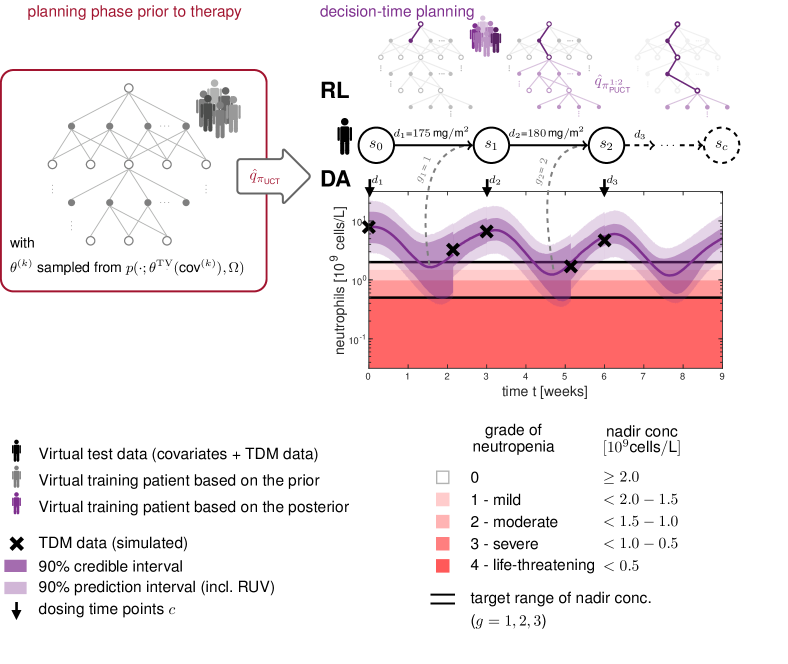
Figure 3: The interplay of data assimilation (DA) and reinforcement learning (RL). In the planning phase prior to therapy, the expected long-term return $q_{\pi_{0}}:=\hat{q}_{\pi_{\text{UCT}}}$ is estimated in Monte Carlo Tree search (MCTS) with upper confidence bound applied to trees (UCT) using an ensemble of covariates $\text{cov}^{(k)}$ and parameter values $\theta^{(k)}\sim p(\cdot|\theta^{\textrm{TV}}(\text{cov}^{(k)}),\Omega)$. The first dose is selected based on $q_{\pi_{0}}:=\hat{q}_{\pi_{\text{UCT}}}$ for the patient specific covariate class. The DA algorithm initializes a particle ensemble given the patient’s covariates cov. The ensemble is propagated forward continuously in time, and observed patient TDM data (black crosses) is assimilated when it becomes available. This results in updated uncertainty, visible as ’cuts’ in the credible/prediction intervals. In contrast, the RL state evolves in discrete time steps $c$ according to the decision time points and only considers selected features/summaries of the model state of the patient, e.g., smoothed posterior expectation of nadir concentrations translated into neutropenia grades. At each decision time point, the posterior model state of the patient is used to refine the prior computed $\hat{q}_{\pi_{\text{UCT}}}$ (grey tree) for future reachable states (light purple tree). This individualizes the tree based on individualized uncertainties ($\mathcal{E}_{1:c}$).

Since the refinement as well as the DA part has to run in real time (online), it has to be performed efficiently. We do not need to take all possible state combinations into account, but only those that are still relevant for the remaining part of the therapy. This reduces the computational effort, in particular for later cycles. The proposed DA-RL approach results in a sequence of estimated optimal dosing policies $\widehat{\pi}^{1},\widehat{\pi}^{1:2},\dots$ with $\widehat{\pi}^{1:c}$ denoting the estimated optimal dosing policy based on TDM data $y_{1:c}$, i.e. based on $\mathcal{E}_{1:c}$. In addition, we do not need to estimate the individualized action-value function from scratch, but can exploit $q_{\pi_{0}}:=\hat{q}_{\pi_{\text{UCT}}}$ as a prior determined by the RL scheme prior to any TDM data (see paragraph following Eq. (14)). In PUCT (predictor+UCT [27, 42]), the exploitation vs. exploration parameter $\epsilon_{c}$ in Eq. (14) is modified to prioritize doses with high a-priori expected long-term return:

$$U_{k}(s_{c},d)=\underbrace{q^{1:c}_{{k}}(s_{c},d)\vphantom{\frac{\sqrt{\sum_{d^{\prime}}N^{(k)}(s_{c},d^{\prime})}}{N^{(k)}(s_{c},d)+1}}}_{\text{exploitation}}+\,\epsilon_{c}\cdot\underbrace{\frac{\exp\!\big{(}\hat{q}_{\pi_{UCT}}(s,d)\big{)}}{\sum_{d^{\prime}}\exp\!\big{(}\hat{q}_{\pi_{UCT}}(s,d^{\prime})\big{)}}}_{\text{priortising}}\underbrace{\frac{\sqrt{N_{k}(s_{c})}}{N_{k}(s_{c},d)+1}}_{\text{exploration}}.$$ (17)

Finally, we define $\widehat{\pi}^{1:c}_{\text{PUCT}}=\pi^{1:c}_{K}$ based on $\mathcal{E}_{1:c}$ as an estimate of the optimal individualized dosing policy in the training setting (using Eqs. (13)+(17)), and $\hat{q}_{\pi_{\text{PUCT}}^{c}}=q_{K}$ as an estimate of the associated expected long term return based on $\mathcal{E}_{1:c}$. For individualized dose recommendations in a clinical TDM setting, we again use $\pi^{*}=\text{arg max }\hat{q}_{\pi_{\text{PUCT}}^{1:c}}$, i.e., $\epsilon_{c}=0$ in Eq. (17). See Figure 3 and 4, and Section S 7.

Figure 4: Pseudo Code of DA-RL-guided dosing. At therapy start a particle ensemble $\mathcal{E}_{0}$ for the sequential data assimilation (DA) approach is sampled from the prior parameter distribution given the patient’s covariates. Then for the initial state $s_{0}$ (pretreatment) the first dose is selected according to the prior expected long-term return $q_{\pi_{0}}:=\hat{q}_{\pi_{\text{UCT}}}$ calculated beforehand in the prior planning phase (Monte Carlo Tree Search (MCTS) with upper confidence bound applied to trees (UCT)). The selected dose is given to the patient and patient-specific therapeutic drug/biomarker monitoring (TDM) data $y_{c}$ is collected within cycle $c$. The TDM data is assimilated via a sequential DA approach (particle filter and smoother) creating a posterior particle ensemble $\mathcal{E}_{1:c}$. For subsequent dose decisions ($c=1,\dots,C$). The new patient state is inferred using $\mathcal{E}_{1:c}$, e.g., smoothed posterior expectation of the nadir concentration translated into the neutropenia grade of the cycle. Then a MCTS is started from the current patient state using $\mathcal{E}_{1:c}$ in the model simulations. Within the tree search we use the PUCT algorithm with prioritized exploration based on $\hat{q}_{\pi_{\text{UCT}}}$.

3 RESULTS

3.1 Novel individualized dosing strategies decreased the occurrence of
grade 4 and grade 0 neutropenia compared to existing approaches

We compared our proposed approaches with existing approaches for MIPD based on simulated TDM data in paclitaxel-based chemotherapy. The design was chosen to correspond to the CEPAC-TDM study [14]: neutrophil counts at day 0 and 15 of each cycle were simulated for virtual patients employing a PK/PD model for paclitaxel-induced cumulative neutropenia (Figure S 1) [29]. We focused only on paclitaxel dosing; we did not take into account drop-outs, dose reductions due to non-haematological toxicities, adherence and comedication. Occurrence of grade 4 neutropenia, therefore, differed between our simplified simulation study and the clinical study (as might be expected), see Section S 8.2. This should be taken into account when interpreting the results. To obtain meaningful statistics, all analyses were repeated $N=1000$ times with covariates sampled from the observed covariate ranges in the CEPAC-TDM study. Detailed discussions and further analyses are provided in Section S 2 and S 8.

Figure 5 shows the predicted neutrophil concentrations—median & 90% confidence interval (CI)—over six cycles of three weeks each. A successful neutrophil-guided dosing should result in nadir concentrations within the target range (grades 1-3, between black horizontal lines). In all cycles, PK-guided dosing prevented the nadir concentrations (90% CI) to drop as low as for the standard dosing (Figure 5 A). However, PK-guided dosing also increased the occurrence of grade 0 (Figure 6).

RL-guided dosing controlled the neutrophil concentration well across the cycles (Figure 5 B) and the distribution of nadir concentrations over the whole population was increasingly concentrated within the target range (panel F). The occurrence of grade 0 and 4 neutropenia was substantially reduced compared to standard and PK-guided dosing (Figure 6).

For MAP-guided dosing, the occurrence of grade 4 neutropenia increased over the cycles (Figure 6), showing the typical cumulative trend of neutropenia [29], despite inclusion of TDM data. In contrast, DA steadily guided nadir concentrations into the target range (Figure 5 D and F), thereby substantially decreasing the variance, i.e., the variability in outcome. The occurrence of grade 0 and 4 was reduced considerably in later cycles (Figure 6), suggesting that individualized uncertainty quantification played a crucial role in reducing the variability in outcome.

Integrating individualized uncertainties and considering the model state of the patient in the RL approach (DA-RL-guided dosing) also moved nadir concentrations into the target range and clearly decreased the variance (Figure 5 B+F). The slight differences between DA and DA-RL (Figure 6) might be related to the difference in weighting grade 0 and 4 in the respective reward functions (eq. (16) vs. eq. (7)). For additional comparisons, see Figure S 22.

In summary, individualized uncertainties as in DA- and DA-RL-guided dosing seemed to be crucial in bringing nadir concentrations into the target range and reducing the variability of the outcome, thus achieving the goal of therapy individualization. For this specific example, both approaches showed comparable results, but DA-RL has the greater potential for long-term optimization in a delayed feedback environment as well as integrating multiple endpoints.

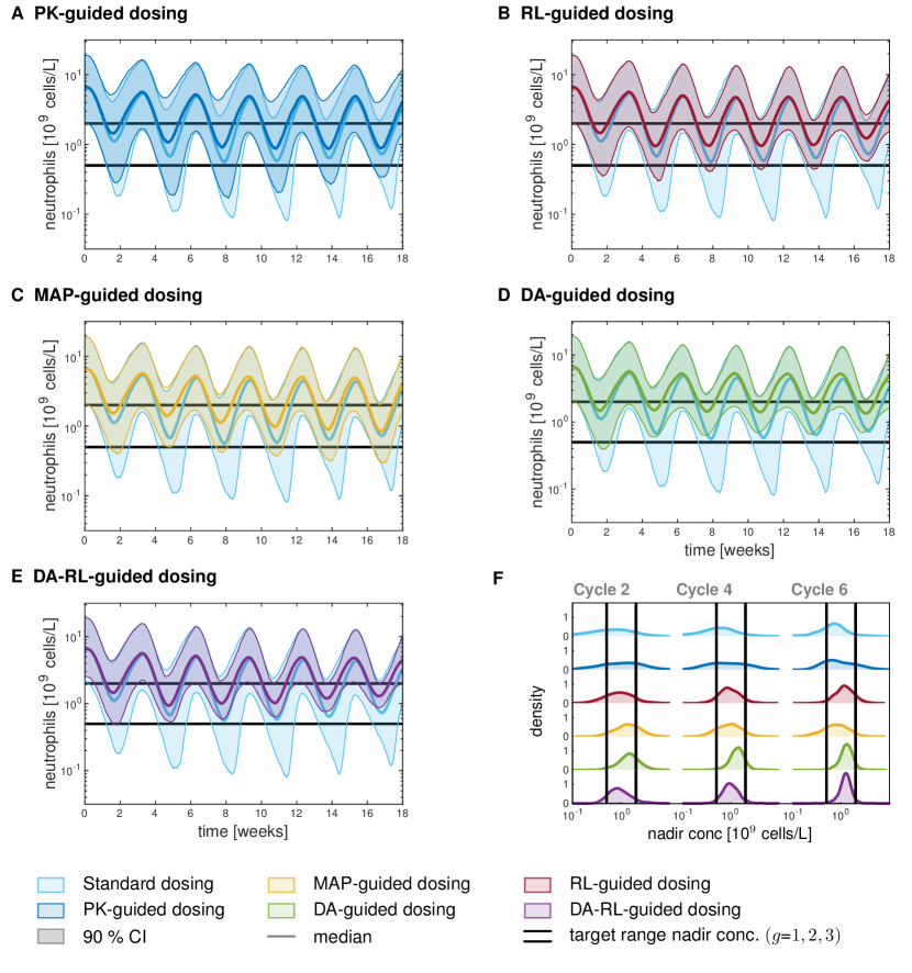
Figure 5: Comparison of different dosing policies for paclitaxel dosing. Comparison of the 90 % confidence intervals and median of the neutrophil concentration for the test virtual population ($N=1000$) using (A) PK-guided dosing (B) RL-guided dosing (C) MAP-guided dosing, (D) DA-guided dosing, and (E) DA-RL-guided dosing, each in comparison to the standard dosing (BSA-based dosing). PK-guided dosing is the only approach that also takes into account exposure data ($T_{C_{\text{drug}}\geq 0.05\,\mu\text{mol}/\text{L}}$). (F) Comparison of the distributions of model-predicted nadir concentrations (smooth by kernel density estimation) for the test virtual population ($N=1000$).

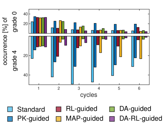
Figure 6: Occurrence of grade 0 and grade 4 for the different dosing policies. The percentage is based on a test virtual population ($N=1000$) and six cycles (inferred from the model predicted nadir concentration). Additional analyses is provided in the supplement, Figure S 22.

3.2 Identification of relevant covariates via investigating the expected long-term return in RL

A key object in RL is the expected long-term return or action-value function $q_{\pi}(s,d)$ (see eq. 10). We demonstrate that it contains important information to identify relevant covariates to individualize dosing.

Figure 7 A shows the estimated action-value function for RL-guided dosing stratified for the covariates, sex, age and baseline neutrophil counts $\text{ANC}_{0}$ (covariate classes are shown in the legend) for the first cycle dose selection. $\text{ANC}_{0}$ was found to be by far the most important characteristic for the RL-based dose selection at therapy start. Differences in age and sex played only minor roles. For comparison, the first cycle dose selection in the PK-guided algorithm is only based on sex and age. The steepness of the curves gives an idea about the robustness of the dose selection. For the second dose selection, the grade of neutropenia in the first cycle ($g_{1}$) has the largest impact, while larger $\text{ANC}_{0}$ led to larger optimal doses (Figure 7 B). To illustrate the dose selection in RL, we extracted a similar decision tree to the one developed by Joerger et al. [13], see Figure S 13.

Similar investigations are not straightforward for MAP- or DA-guided dosing as no means is provided to investigate dose recommendations for an entire population; these approaches optimize doses for a single patient.

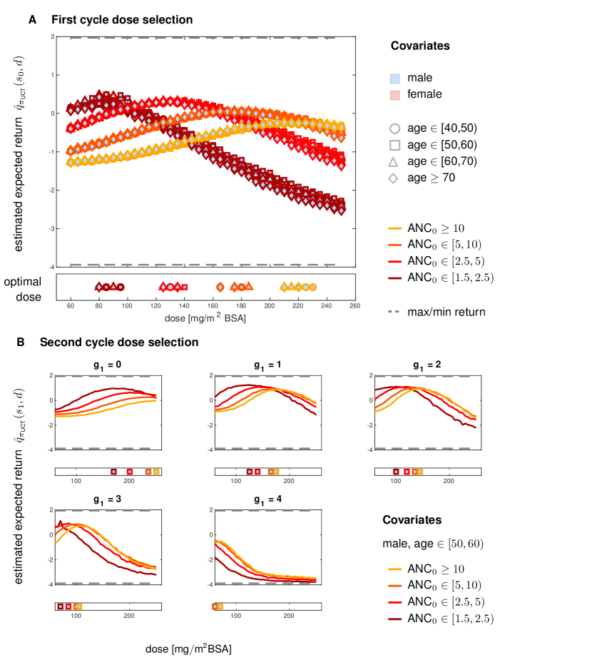
Figure 7: Expected long-term return across the dose range for dose selection. A across the considered covariate combinations for the dose selection in cycle 1. The symbols plotted below the x-axis show the optimal dose for the corresponding covariate class (i.e. the arg max of the plotted line). B for fixed sex and age class (here, male between 50 and 60 years) with different pre-treatment neutrophil values $\text{ANC}_{0}$ and observed neutropenia grades in cycle 1, i.e., $\text{g}_{1}$. The optimal dose for the second cycle depends on the neutropenia grade of the previous cycle and the pre-treatment neutrophil count $\text{ANC}_{0}$ in $[10^{9}\text{cells}/\text{L}]$. The grey dashed line shows the maximum and minimum possible return from the first cycle (A) and the second cycle (B) onwards, with $\gamma=0.5$. The covariate classes were chosen based on the CEPAC-TDM study population: inclusion criteria were $\text{ANC}_{0}>\cdot 1.5\cdot 10^{9}\text{cells}/\text{L}$; the typical baseline count for male was $\text{ANC}_{0}=6.48\cdot 1.5\cdot 10^{9}\text{cells}/\text{L}$ (arm B). The median age was $63$ years ranging from 51 to 74 years (5th and 95th percentile of the population in arm B), see [38, 14].

4 DISCUSSION

We present three promising MIPD approaches employing DA and/or RL that substantially reduced the number of (virtual) patients in life-threatening grade 4 and grade 0, a surrogate marker for efficacy of the anticancer treatment.

RL-guided dosing in oncology has been proposed before [25], however, only considering the mean tumor diameter. Since only a marker for efficacy was considered this led to a one-sided dosing scheme and resulted in very high optimal doses. The authors therefore introduced action-derived rewards, i.e., penalties on high doses. In contrast, neutrophil-guided dosing considers toxicity and efficacy (link to median survival) simultaneously. Ideally, dosing decisions should also include other adverse effects, e.g., peripheral neuropathy, tumor response or long-term outcomes, e.g., overall or progression free survival. Notably, RL easily extends to multiple adverse/beneficial effects and is especially suited for time-delayed feedback environments [23, 34], as typical in many diseases.

Using MCTS with UCT, we employed an RL framework that exploits the possibility to simulate until the end of therapy and evaluate the return. Consequently, it requires less approximations as temporal difference approaches (e.g., Q-learning, used in [25]) that avoid computation of the return via a decomposition (Bellman equation). Moreover, exploration via UCT allows to systematically sample from the dose range (as opposed to an $\epsilon$-greedy strategy) and allows to include additional information, e.g., uncertainties or prior information (as in PUCT). This becomes key when combined with direct RL based on real-world patient data, see e.g. [43, 44], which would allow to compensate for a potential model bias. At the end of a patient’s therapy the observed return can be evaluated and used to update the expected return $\hat{q}_{\widehat{\pi}}$. This update would even be possible if the physician did not follow the dose recommendation (off-policy learning) and could be implemented across clinics, as it could be done locally without exchanging patient data. Thus, the presented approach builds a basis for continuous learning post-approval, which has the potential to substantially improve patient care, including patient subgroups underrepresented in clinical studies.

Overall we have shown that DA and RL techniques can be seamlessly integrated and combined with existing NLME and data analysis frameworks for a more holistic approach to MIPD. Our study demonstrates that incorporation of individualized uncertainties (as in DA) is favorable over state-of-the-art online algorithms such as MAP-guided dosing. The integrated DA-RL framework allows not only to consider prior knowledge from clinical studies but also to improve and individualize the model and the dosing policy simultaneously during the course of treatment by integrating patient-specific TDM data. Thus, the combination provides an efficient and meaningful alternative to solely DA-guided dosing, as it allocates computational resources between online and offline and the RL part provides an additional layer of learning to the model (in form of the expected long-term return) that can be used to gain deeper insights into important covariates for the dose selection. Therefore showing that RL approaches can be well interpreted in clinically relevant terms, e.g., highlighting the role of ANC₀ values. Well-informed and efficient MIPD bears huge potential in drug-development as well as in clinical practice as it could (i) increase response rates in clinical studies [1], (ii) facilitate recruitment by relaxing exclusion criteria [3], (iii) enable continuous learning post-approval and thus improve treatment outcomes in the long-term.

Author Contributions

C.M., N.H., C.K., W.H., J.dW. designed research, C.M. mainly performed the research, C.M., N.H., C.K., W.H., J.dW. analyzed data and wrote the manuscript.

References

- [1] Peck, R.W. The right dose for every patient : a key step for precision medicine. Nat. Rev. Drug Discov. (2015). doi:10.1038/nrd.2015.22.
- [2] de Jonge, M.E., Huitema, A.D.R., Schellens, J.H.M., & Rodenhuis, S. Individualised Cancer Chemotherapy : Strategies and Performance of Prospective Studies on Therapeutic Drug Monitoring with Dose Adaptation. A Review. Clin Pharmacokinet 44, 147–173 (2005).
- [3] Darwich, A.S. et al. Why Has Model-Informed Precision Dosing Not Yet Become Common Clinical Reality? Lessons From the Past and a Roadmap for the Future. Clin. Pharmacol. Ther. 101, 646–656 (2017). doi:10.1002/cpt.659.
- [4] Crawford, J., Dale, D.C., & Lyman, G.H. Chemotherapy-induced neutropenia. Cancer 100, 228–237 (2004). doi:10.1002/cncr.11882.
- [5] National Cancer Institute. Common terminology criteria for adverse events (CTCAE) version 4.03. Bethesda, Maryl. 1–194 (2010).
- [6] Cameron, D.A., Massie, C., Kerr, G., & Leonard, R.C. Moderate neutropenia with adjuvant CMF confers improved survival in early breast cancer. Br. J. Cancer 89, 1837–1842 (2003). doi:10.1038/sj.bjc.6601366.
- [7] Di Maio, M. et al. Chemotherapy-induced neutropenia and treatment efficacy in advanced non-small-cell lung cancer: a pooled analysis of three randomised trials. Lancet Oncol. 6, 669–677 (2005). doi:10.1016/S1470-2045(05)70255-2.
- [8] Di Maio, M., Gridelli, C., Gallo, C., & Perrone, F. Chemotherapy-induced neutropenia: a useful predictor of treatment efficacy? Nat. Clin. Pract. Oncol. 3, 114–115 (2006). doi:10.1038/ncponc0445.
- [9] Wallin, J.E., Friberg, L.E., & Karlsson, M.O. A tool for neutrophil guided dose adaptation in chemotherapy. Comput. Methods Programs Biomed. 93, 283–291 (2009). doi:10.1016/j.cmpb.2008.10.011.
- [10] Hansson, E.K., Wallin, J.E., Lindman, H., Sandström, M., Karlsson, M.O., & Friberg, L.E. Limited inter-occasion variability in relation to inter-individual variability in chemotherapy-induced myelosuppression. Cancer Chemother. Pharmacol. 65, 839–848 (2010). doi:10.1007/s00280-009-1089-3.
- [11] Netterberg, I., Nielsen, E.I., Friberg, L.E., & Karlsson, M.O. Model-based prediction of myelosuppression and recovery based on frequent neutrophil monitoring. Cancer Chemother. Pharmacol. 80, 343–353 (2017). doi:10.1007/s00280-017-3366-x.
- [12] Peters, S. et al. Metastatic non-small-cell lung cancer (NSCLC): ESMO Clinical Practice Guidelines for diagnosis, treatment and follow-up. Ann. Oncol. 23 (2012). doi:10.1093/annonc/mds226.
- [13] Joerger, M. et al. Evaluation of a pharmacology-driven dosing algorithm of 3-weekly paclitaxel using therapeutic drug monitoring: A pharmacokinetic-pharmacodynamic simulation study. Clin. Pharmacokinet. 51, 607–617 (2012). doi:10.2165/11634210-000000000-00000.
- [14] Joerger, M. et al. Open-label, randomized study of individualized, pharmacokinetically (PK)-guided dosing of paclitaxel combined with carboplatin or cisplatin in patients with advanced non-small-cell lung cancer (NSCLC). Ann. Oncol. 27, 1895–1902 (2016). doi:10.1093/ANNONC/MDW290.
- [15] Keizer, R.J., Heine, R., Frymoyer, A., Lesko, L.J., Mangat, R., & Goswami, S. Model-Informed Precision Dosing at the Bedside : Scientific Challenges and Opportunities. CPT Pharmacometrics Syst. Pharmacol. 785–787 (2018). doi:10.1002/psp4.12353.
- [16] Sheiner, L.B., Beal, S., Rosenberg, B., & Marathe, V.V. Forecasting individual pharmacokinetics. Clin. Pharmacol. Ther. 26, 294–305 (1979). doi:10.1002/cpt1979263294.
- [17] Wallin, J.E., Friberg, L.E., & Karlsson, M.O. Model-based neutrophil-guided dose adaptation in chemotherapy: Evaluation of predicted outcome with different types and amounts of information. Basic Clin. Pharmacol. Toxicol. 106, 234–242 (2009). doi:10.1111/j.1742-7843.2009.00520.x.
- [18] Bleyzac, N. et al. Improved clinical outcome of paediatric bone marrow recipients using a test dose and Bayesian pharmacokinetic individualization of busulfan dosage regimens. Bone Marrow Transplant. 28, 743–751 (2001). doi:10.1038/sj.bmt.1703207.
- [19] Wallin, J.E., Friberg, L.E., & Karlsson, M.O. Model Based Neutrophil Guided Dose Adaptation in Chemotherapy ; Evaluation of Predicted Outcome with Different Type and Amount of Information. In Page Meet. (2009).
- [20] Holford, N. Pharmacodynamic principles and target concentration intervention. Transl. Clin. Pharmacol. 26, 150–154 (2018). doi:10.12793/tcp.2018.26.4.150.
- [21] Maier, C., Hartung, N., Wiljes, J., Kloft, C., & Huisinga, W. Bayesian Data Assimilation to Support Informed Decision Making in Individualized Chemotherapy. CPT Pharmacometrics Syst. Pharmacol. 9, 153–164 (2020). doi:10.1002/psp4.12492.
- [22] Zhao, Y., Zeng, D., Socinski, M.A., & Kosorok, M.R. Reinforcement learning strategies for clinical trials in nonsmall cell lung cancer. Biometrics 67, 1422–1433 (2011). doi:10.1111/j.1541-0420.2011.01572.x.
- [23] Yu, C., Liu, J., & Nemati, S. Reinforcement Learning in Healthcare: A Survey. arXiv (2019).
- [24] Escandell-Montero, P. et al. Optimization of anemia treatment in hemodialysis patients via reinforcement learning. Artif. Intell. Med. 62, 47–60 (2014). doi:10.1016/j.artmed.2014.07.004.
- [25] Yauney, G. & Shah, P. Reinforcement Learning with Action-Derived Rewards for Chemotherapy and Clinical Trial Dosing Regimen Selection. Proc. Mach. Learn. Res. 85 (2018).
- [26] Silver, D. et al. Mastering the game of Go with deep neural networks and tree search. Nature 529, 484–489 (2016). doi:10.1038/nature16961.
- [27] Rosin, C.D. Multi-armed bandits with episode context. Ann. Math. Artif. Intell. 61, 203–230 (2011). doi:10.1007/s10472-011-9258-6.
- [28] Friberg, L.E., Henningsson, A., Maas, H., Nguyen, L., & Karlsson, M.O. Model of Chemotherapy-Induced Myelosuppression With Parameter Consistency Across Drugs. J. Clin. Oncol. 20, 4713–4721 (2002). doi:10.1200/JCO.2002.02.140.
- [29] Henrich, A. et al. Semimechanistic Bone Marrow Exhaustion Pharmacokinetic/Pharmacodynamic Model for Chemotherapy-Induced Cumulative Neutropenia. J. Pharmacol. Exp. Ther. 362, 347–358 (2017). doi:10.1124/jpet.117.240309.
- [30] Huizing, M.T. et al. Pharmacokinetics of paclitaxel and carboplatin in a dose-escalating and dose-sequencing study in patients with non-small-cell lung cancer. J. Clin. Oncol. 15, 317–329 (1997). doi:10.1200/JCO.1997.15.1.317.
- [31] Keizer, R.J. et al. Get Real: Integration of Real-World Data to Improve Patient Care. Clin. Pharmacol. Ther. 0, 4–7 (2020). doi:10.1002/cpt.1784.
- [32] Sheiner, L.B. Learning versus confirming in clinical drug development. Clin. Pharmacol. Ther. 61, 275–291 (1997). doi:10.1016/S0009-9236(97)90160-0.
- [33] Bertsekas, D.P. Reinforcement Learning and Optimal Control, (Athena Scientific2019).
- [34] Zhavoronkov, A., Vanhaelen, Q., & Oprea, T.I. Will Artificial Intelligence for Drug Discovery Impact Clinical Pharmacology? Clin. Pharmacol. Ther. 0 (2020). doi:10.1002/cpt.1795.
- [35] Sutton, R.S. & Barto, A.G. Reinforcement Learning An Introduction. 2nd edn., (The MIT Press, Cambridge, MA2018).
- [36] Bartolucci, R. et al. Artificial intelligence and machine learning : just a hype or a new opportunity for pharmacometrics ? In Page Meet. 28 Stock. Abstr 9148 (2019).
- [37] Ribba, B., Dudal, S., Lavé, T., & Peck, R.W. Model‐Informed Artificial Intelligence: Reinforcement Learning for Precision Dosing. Clin. Pharmacol. Ther. 0, 1–5 (2020). doi:10.1002/cpt.1777.
- [38] Henrich, A. Pharmacometric modelling and simulation to optimise paclitaxel combination therapy based on pharmacokinetics , cumulative neutropenia and efficacy. Ph.D. thesis, Freie Universität Berlin (2017). doi:10.17169/refubium-12511.
- [39] Auer, P., Cesa-Bianchi, N., & Fischer, P. Finite-time Analysis of the Multiarmed Bandit Problem. Mach. Learn. 47, 235–256 (2002). doi:10.1023/A:1013689704352.
- [40] Coulom, R. Efficient Selectivity and Backup Operators in Monte-Carlo Tree Search. In 5th Int. Conf. Comput. Games, 72–83 (2007). doi:10.1007/978-3-540-75538-8˙7.
- [41] Kocsis, L. & Szepesvári, C. Bandit Based Monte-Carlo Planning. ECML 282–293 (2006).
- [42] Silver, D. et al. Mastering the game of Go without human knowledge. Nat. Publ. Gr. 550, 354–359 (2017). doi:10.1038/nature24270.
- [43] Sutton, R.S. Dyna , an Integrated Architecture for Learning , Planning , and Reacting. Work. Notes 1991 AAAI Spring Symp. SIGART Bull. 151–155 (1991).
- [44] Silver, D., Sutton, R.S., & Martin, M. Sample-Based Learning and Search with Permanent and Transient Memories. In Proc. 25th Int. Conf. Mach. Learn. Helsinki, Finl. (2008).