SSumM: Sparse Summarization of Massive Graphs

Abstract.

Given a graph $G$ and the desired size $k$ in bits, how can we summarize $G$ within $k$ bits, while minimizing the information loss?

Large-scale graphs have become omnipresent, posing considerable computational challenges. Analyzing such large graphs can be fast and easy if they are compressed sufficiently to fit in main memory or even cache. Graph summarization, which yields a coarse-grained summary graph with merged nodes, stands out with several advantages among graph compression techniques. Thus, a number of algorithms have been developed for obtaining a concise summary graph with little information loss or equivalently small reconstruction error. However, the existing methods focus solely on reducing the number of nodes, and they often yield dense summary graphs, failing to achieve better compression rates. Moreover, due to their limited scalability, they can be applied only to moderate-size graphs.

In this work, we propose SSumM, a scalable and effective graph-summarization algorithm that yields a sparse summary graph. SSumM not only merges nodes together but also sparsifies the summary graph, and the two strategies are carefully balanced based on the minimum description length principle. Compared with state-of-the-art competitors, SSumM is (a) Concise: yields up to $11.2\times$ smaller summary graphs with similar reconstruction error, (b) Accurate: achieves up to $4.2\times$ smaller reconstruction error with similarly concise outputs, and (c) Scalable: summarizes $26\times$ larger graphs while exhibiting linear scalability. We validate these advantages through extensive experiments on $10$ real-world graphs.

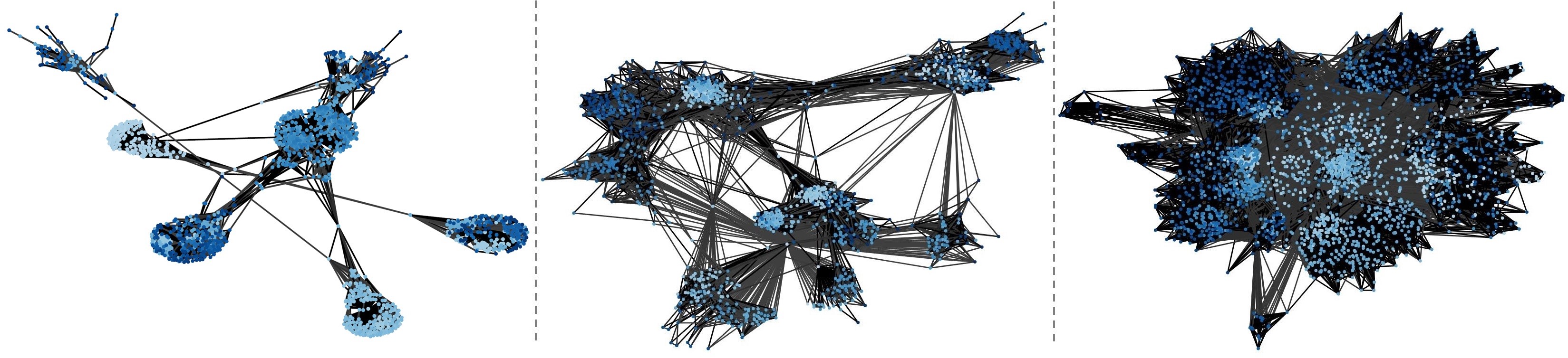
Figure 1. SSumM gives sparse and concise summary graphs. The reconstruction errors of the above summary graphs, obtained by different algorithms, are similar ($\pm 5\%$).

1. Introduction

Graphs are a fundamental abstraction that is widely used to represent a variety of relational datasets. As the underlying data are accumulated rapidly, massive graphs have appeared, such as (a) $3.5$ billion web pages with $128$ billion hyperlinks (Meusel et al., 2015), (b) professional networks with more than $20$ billion connections (Shin et al., 2019), and (c) social networks with hundreds of billions of connections (Ching et al., 2015).

Despite the abundance of massive graphs, many existing graph-analysis tools are inapplicable to such graphs since their computational costs grow rapidly with the size of graphs. Moreover, massive graphs often do not fit in main memory, causing I/O delays over the network or to the disk.

These problems can be addressed by graph summarization, which aims to preserve the essential structure of a graph while shrinking its size by removing minor details. Given a graph $G=(V,E)$ and the desired size $k$, the objective of the graph summarization problem is to find a summary graph $\overline{G}=(S,P,\omega)$ of size $k$ from which $G$ can be accurately reconstructed. The set $S$ is a set of supernodes, which are distinct and exhaustive subsets of nodes in $G$, and the set $P$ is a set of superedges (i.e., edges between supernodes). The weight function $\omega$ assigns an integer to each superedge. Given the summary graph $\overline{G}$, we reconstruct a graph $\hat{G}$ by connecting all pairs of nodes belonging to the source and destination supernodes of each superedge and assigning a weight, computed from the weight of the superedge, to each created edge. Note that $\hat{G}$ is not necessarily the same with $G$, and we call their similarity the accuracy of $\overline{G}$.

Graph summarization stands out among a variety of graph-compression techniques (relabeling nodes (Boldi and Vigna, 2004; Apostolico and Drovandi, 2009; Chierichetti et al., 2009), encoding frequent substructures with few bits (Buehrer and Chellapilla, 2008; Khan et al., 2015), etc.) due to the following benefits: (a) Elastic: we can reduce the size of outputs (i.e., a summary graph) as much as we want at the expense of increasing reconstruction errors. (b) Analyzable: since the output of graph summarization is also a graph, existing graph analysis and visualization tools can easily be applied. For example, (Riondato et al., 2017; LeFevre and Terzi, 2010; Beg et al., 2018) compute adjacency queries, PageRank (Page et al., 1999), and triangle density (Tsourakakis, 2015) directly from summary graphs, without restoring the original graph. (c) Combinable for Additional Compression: due to the same reason, the output summary graph can be further compressed using any graph-compression techniques.

While a number of graph-summarization algorithms (LeFevre and Terzi, 2010; Riondato et al., 2017; Beg et al., 2018) have been developed for finding accurate summary graphs (i.e., those with low reconstruction errors) and eventually realizing the above benefits, they share common limitations. First, their scalability is severely limited, and they cannot be applied to billion-scale graphs for which graph summarization can be extremely useful. Specifically, the largest graph to which they were applied has only about $3$ million nodes and $34$ million edges, which take only about $23.8$MB (Beg et al., 2018). More importantly, existing algorithms are not effective in reducing the size in bits of graphs since they solely focus on reducing the number of nodes (see Fig. 1). Surprisingly, the size in bits of summary graphs often exceeds that of the original graphs, as reported in (Riondato et al., 2017) and shown in our experiments.

To address these limitations, we propose SSumM (Sparse Summar-ization of Massive Graphs), a scalable graph-summarization algorithm that yields concise but accurate summary graphs. SSumM focuses on minimizing reconstruction errors while limiting the size in bits of the summary graph, instead of the number of nodes. Moreover, to co-optimize the compactness and accuracy, SSumM carefully combines nodes and at the same time sparsifies edges. Lastly, for scalability, SSumM rapidly searches promising candidate pairs of nodes to be merged. As a result, SSumM significantly outperforms its state-of-the-art competitors in terms of scalability and the compactness and accuracy of outputs.

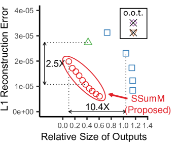
(a) Compactness and Accuracy

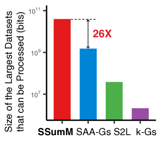
(b) Scalability

Figure 2. Advantages of SSumM. Compared to its state-of-the-art competitors, SSumM yields more compact and accurate summary graphs, and it successfully processes a $\mathbf{26\times}$ larger dataset with $\mathbf{0.8}$ billion edges. See Sect. 4 for details.

In summary, our contributions in this work are as follows:

• Practical Problem Formulation: We introduce a new practical variant (Problem 1) of the graph summarization problem, where the size in bits of outputs (instead of the number of supernodes) is constrained so that the outputs easily fit target storage.

• Scalable and Effective Algorithm Design: We propose SSumM for the above problem. Compared to its state-of-the-art competitors, SSumM handles up to $\mathbf{26\times}$ larger graphs with linear scalability, and it yields up to $\mathbf{11.2\times}$ smaller summary graphs with similar reconstruction errors (Fig. 2 and Thm. 3.4).

• Extensive Experiments: Throughout extensive experiments on 10 real-world graphs, we validate the advantages of SSumM over its state-of-the-art competitors.

Reproducibility: The source code and datasets used in the paper can be found at http://dmlab.kaist.ac.kr/ssumm/.

In Sect. 2, we introduce some notations and concepts, and we formally define the problem of graph summarization within the given size in bits. In Sect. 3, we present SSumM, our proposed algorithm for the problem, and we analyze its time and space complexity. In Sect. 4, we evaluate SSumM through extensive experiments. After discussing related work in Sect. 5, we draw conclusions in Sect. 6.

Table 1. Symbols and Definitions.

Symbol	Definition
Symbols for the problem definition (Sect. 2)
$G=(V,E)$	input graph with subnodes $V$ and subedges $E$
$A$	adjacency matrix of $G$
$\overline{G}=(S,P,\omega)$	summary graph with supernodes $S$, superedges $P$,
	and a weight function $\omega$
$V_{u}$	supernode with the subnode $u$
$\Pi_{S}$	set of all unordered pairs of supernodes
$E_{AB}$	set of subedges between the supernodes $A$ and $B$
$\Pi_{AB}$	set of all possible subedges between the supernodes $A$ and $B$
$\hat{G}=(V,\hat{E},\hat{\omega})$	reconstructed graph with subnodes $V$, subedges $\hat{E}$,
	and a weight function $\hat{\omega}$
$\hat{A}$	weighted adjacency matrix of $\hat{G}$
$k$	desired size in bits of the output summary graph
Symbols for the proposed algorithm (Sect. 3)
$T$	given number of iterations
$\theta(t)$	threshold at the $t$-th iteration
$\mathcal{S}_{t}$	set of candidate sets at the $t$-th iteration

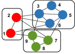
(a) Input graph $G$

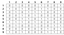
(b) Adjacency matrix $A$

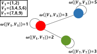
(c) Summary graph $\overline{G}$

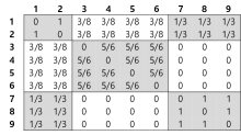
(d) Reconstructed adjacency matrix $\hat{A}$

Figure 3. Illustration of graph summarization. An example graph $G$ in (a) has the adjacency matrix $A$ in (b). From a summary graph $\overline{G}$ in (c), we restore a graph $\hat{G}$, whose weighted adjacency matrix is $\hat{A}$ in (d). Each subnode in $G$ belongs to one supernode in $\hat{G}$, and the weight of each superedge corresponds to the number of subedges between the two supernodes. For example, since there are $3$ subedges (i.e., $\{1,6\}$, $\{2,3\}$, $\{2,6\}$) between supernodes $V_{1}$ and $V_{3}$, the weight $\omega(\{V_{1},V_{3}\})$ of the superedge $\{V_{1},V_{3}\}$ is $3$. Note that two supernodes do not have to be connected by a superedge even when there are subedges between them (see $V_{3}$ and $V_{7}$). Eq. (1) is used for the weights of subedges in $\hat{G}$. For example, the weight $\hat{\omega}(\{1,3\})$ of the subedge $\{1,3\}$ in $\hat{G}$ is $\frac{\omega(\{V_{1},V_{3}\})}{|\Pi_{V_{1}V_{3}}|}=\frac{3}{8}$.

2. Preliminaries & Problem Definition

We introduce some notations and concepts that are used throughout this paper. Then, we define the problem of summarizing a graph within the given size in bits. Table 1 lists some frequently-used notations, and Fig. 3 illustrates some important concepts.

2.1. Notations and Concepts

Input graph: Consider an undirected graph $G=(V,E)$ with nodes $V$ and edges $E$. Each edge $\{u,v\}\in E$ joins two distinct nodes $u\neq v\in V$. We assume that $G$ is undirected without self-loops for simplicity, while the considered problem and our proposed algorithm can easily be extended to directed graphs with self-loops. We call nodes and edges in $G$ subnodes and subedges, respectively, to distinguish them from those in summary graphs, described below.

Summary graph: A summary graph $\overline{G}=(S,P,\omega)$ of a graph $G=(V,E)$ consists of a set $S$ of supernodes, a set $P$ of superedges, and a weight function $\omega$. The supernodes $S$ are distinct and exhaustive subsets of $V$, i.e., $\bigcup_{A\in S}A=V$ and $A\cap B=\emptyset$ for all $A\neq B\in S$. Thus, every subnode in $V$ is contained in exactly one supernode in $S$, and we denote the supernode that each subnode $v\in V$ belongs to as $V_{v}\in S$. Each superedge $\{A,B\}\in P$ connects two supernodes $A,B\in S$, and if $A=B$, then $\{A,B\}=\{A,A\}$ indicates the self-loop at the supernode $A\in S$. We use $\Pi_{S}:={S\choose 2}\cup\{\{A,A\}:A\in S\}$ to denote the all unordered pairs of supernodes, and then $P\subseteq\Pi_{S}$. The weight function $\omega:P\rightarrow\mathbb{Z}^{+}$ assigns to each superedge $\{A,B\}\in P$ the number of subedges between two subnodes belonging to $A\in S$ and $B\in S$, respectively. Let the set of such subedges as $E_{AB}:=\{\{u,v\}\in E:u\in A,v\in B\}$. Then, $\omega(\{A,B\}):=|E_{AB}|$ for each superedge $\{A,B\}\in P$. See Fig. 3 for an example summary graph.

Reconstructed graph: Given a summary graph $\overline{G}=(S,P,\omega)$, we obtain a reconstructed graph $\hat{G}=(V,\hat{E},\hat{\omega})$ conventionally as in (Riondato et al., 2017; LeFevre and Terzi, 2010; Beg et al., 2018). The set $V$ of subnodes is recovered by the union of all supernodes in $S$. The set $\hat{E}$ of subedges is defined as the set of all pairs of distinct subnodes belonging to two supernodes connected by a superedge in $P$. That is, $\hat{E}:=\{\{u,v\}\in V\times V:u\neq v,~{}\{V_{u},V_{v}\}\in P\}$. The weight function $\hat{\omega}:\hat{E}\rightarrow\mathbb{R}^{+}$ is defined as follows:

(1) $$\hat{\omega}(\{u,v\}):=\frac{\omega(\{V_{u},V_{v}\})}{|\Pi_{V_{u}V_{v}}|}=\frac{|E_{V_{u}V_{v}}|}{|\Pi_{V_{u}V_{v}}|},$$

where $\Pi_{V_{u}V_{v}}:=\{\{u,v\}:u\neq v,u\in V_{u},v\in V_{v}\}$ is the set of all possible subedges between two supernodes. That is, in Eq. (1), the denominator is the maximum number of subedges between two supernodes, and each nominator is the actual number of subedges between two supernodes. Note that the graph $\hat{G}$ reconstructed from $\overline{G}$ is not necessarily the same with the original graph $G$, and we discuss how to measure their difference in the following section.

Adjacency matrix: We use $A$ to denote the adjacency matrix of the original graph $G$, and we use $\hat{A}$ to denote the weighted adjacency matrix of a reconstructed graph $\hat{G}$. See Fig. 3 for examples.

2.2. Problem Definition

Now that we have introduced necessary concepts, we formally define, in Problem 1, the problem of graph summarization within the given size in bits. Then, we discuss how we measure the reconstruction error and size of summary graphs. Lastly, we compare the defined problem with the original graph summarization problem.

Problem 1 (Graph Summarization within a Budget in Bits):

• Given: a graph $G=(V,E)$ and the desired size $k$ in bits

• Find: a summary graph $\overline{G}=(S,P,\omega)$

• to Minimize: the reconstruction error

• Subject to: $Size(\overline{G})\leq$ $k$.

Reconstruction error: The reconstruction error corresponds to the difference between the original graph $G$ and the graph $\hat{G}$ reconstructed from the summary graph $\overline{G}$. While there can be many different ways of measuring the reconstruction error, as in the previous studies of graph summarization (Riondato et al., 2017; LeFevre and Terzi, 2010; Beg et al., 2018), we use the $\ell_{p}$ reconstruction error ($RE_{p}$), defined as

(2) $$RE_{p}(G|\overline{G}):=\left(\sum_{i=1}^{\lvert V\rvert}{\sum_{j=1}^{\lvert V\rvert}{\lvert A(i,j)-\hat{A}(i,j)\rvert^{p}}}\right)^{1/p},$$

where $A(i,j)$ is the $(i,j)$-th entry of the matrix $A$. Recall that $A$ and $\hat{A}$ are the (weighted) adjacency matrices of $G$ and $\hat{G}$, respectively.

Size of summary graphs: As in the previous studies (Riondato et al., 2017; LeFevre and Terzi, 2010; Beg et al., 2018), we define the size in bits of (summary) graphs based on the assumption that they are stored in the edge list format. Specifically, the size in bits of the input graph $G=(V,E)$ is defined as

(3) $$Size(G):=2|E|\log_{2}|V|,$$

since each of $|E|$ subedges consists of two subnodes, each of which is encoded using $\log_{2}|V|$ bits. Note that, in order to distinguish $|V|$ items, at least $\log_{2}|V|$ bits per item are required. Similarly, the size in bits of the summary graph $\overline{G}=(S,P,\omega)$ is defined as

(4) $$Size(\overline{G}):=|P|(2\log_{2}|S|+\log_{2}\omega_{max})+|V|\log_{2}|S|,$$

where $\omega_{max}:=\max_{\{A,B\}\in P}\omega(\{A,B\})$ is the maximum superedge weight. The first term in Eq. (4) is for $|P|$ superedges, each of which consists of two supernodes and an edge weight, which are encoded using $2\log_{2}|S|$ bits and $\log_{2}\omega_{max}$ bits, respectively. Again, in order to distinguish $|S|$ (or $\omega_{max}$) items, at least $\log_{2}|S|$ (or $\log_{2}\omega_{max}$) bits are required for encoding each item. The second term in Eq. (4) is for the membership information. Each of $|V|$ nodes belongs to a single supernode, which is encoded using $\log_{2}|S|$ bits.

Comparison with the original problem: Different from Problem 1, where we constrain the size in bits of a summary graph, the number of supernodes is constrained in the original graph summarization problem (LeFevre and Terzi, 2010). By constraining the size in bits, we can easily make summary graphs tightly fit in target storage (main memory, cache, etc.). On the other hand, it is not trivial to control the number of nodes so that a summary graphs tightly fits in target storage. This is because how the size of summary graphs changes depending on the number of supernodes varies across datasets.

3. Proposed Method

We propose SSumM (Sparse Summarization of Massive Graphs), a scalable and effective algorithm for Problem 1. SSumM is a randomized greedy search algorithm equipped with three novel ideas.

One main idea of SSumM is to carefully balance the changes in the reconstruction error and size of the summary graph at each step of the greedy search. To this end, SSumM adapts the minimum description length principle (the MDL principle) (Rissanen, 1978) to measure both the reconstruction error and size commonly in the number of bits. Then, SSumM performs a randomized greedy search, aiming to minimize the total number of bits.

Another main idea of SSumM is to tightly combine two strategies for summarization: merging supernodes into a single supernode, and sparsifying the summary graph. Specifically, instead of creating all possible superedges as long as their weight is not zero, SSumM selectively creates superedges so that its cost function is minimized. SSumM also takes this selective superedge creation into consideration when deciding supernodes to be merged.

Lastly, SSumM achieves linear scalability by rapidly but effectively finding promising candidate pairs of supernodes to be merged.

In this section, we present the cost function (Sect. 3.1) and the search method (Sect. 3.2) of SSumM. After that, we analyze its time and space complexity (Sect. 3.3).

3.1. Cost Function in SSumM

In this subsection, we introduce the cost function, which is used at each step of the greedy search in SSumM. The cost function is for measuring the quality of candidate summary graphs by balancing the size and the reconstruction error, which is important since SSumM aims to reduce the size of the output summary graph while increasing the reconstruction error as little as possible.

For balancing the size and reconstruction error, they need to be directly comparable. To this end, we measure both in terms of the number of bits by adapting the minimum description length principle. The principle states that given data, which is the input graph $G$ in our case, the best model, which is a summary graph $\overline{G}$, for the data is the one that minimizes $Cost(\overline{G},G)$, the description length in bits of $G$ defined as

(5) $$Cost(\overline{G},G):=Cost(\overline{G})+Cost(G|\overline{G}),$$

where the description length is divided into the model cost $Cost(\overline{G})$ and the data cost $Cost(G|\overline{G})$. The model cost measures the number of bits required to describe $\overline{G}$. The data cost measures the number of bits required to describe $G$ given $\overline{G}$ or equivalently to describe the difference between $G$ and $\hat{G}$, which is reconstructed from $\overline{G}$. Thus, the data cost is naturally interpreted as the reconstruction error of $\overline{G}$ in bits. Note that, if $G=\hat{G}$ without any reconstruction error, then $Cost(G|\overline{G})$ becomes zero.

Eq. (5) is the cost function that SSumM uses to balance the size and reconstruction error and thus to measure the quality of candidate summary graphs. Below, we describe each term of Eq. (5) in detail, and then we divide it into the cost for each supernode.

Model cost: For the model cost, we use Eq. (6). It is an upper bound of Eq. (4) which measures the size of a summary graph in bits. In Eq. (6), $\log_{2}|V|$ ($\geq\log_{2}|S|$) and $\log_{2}|E|$ ($\geq\log_{2}\omega_{max}$) bits are used to distinguish supernodes and superedges, respectively. That is,

(6) $$Cost(\overline{G}) :=|P|(2\log_{2}|V|+\log_{2}|E|)+|V|\log_{2}|V|.$$

We divide the total model cost into the model cost for each supernode pair as follows:

(7) $$Cost(\overline{G})=|V|\log_{2}|V|+\sum\nolimits_{\{A,B\}\in\Pi_{S}}Cost(\{A,B\}|\overline{G}),$$

where $Cost(\{A,B\}|\overline{G}):=\mathbb{1}(\{A,B\}\in P)\times(2\log_{2}|V|+\log_{2}|E|)$ is the model cost for each supernode pair $\{A,B\}\in\Pi_{S}$.

Data cost: The data cost $Cost(G|\overline{G})$ is the number of bits required to exactly describe $G$, or equivalently all subedges in $G$, given $\overline{G}$. As explained above, $Cost(G|\overline{G})$ is naturally interpreted as the reconstruction error of $\overline{G}$ in bits. We divide the total data cost into the data cost for each supernode pair as follows:

(8) $$Cost(G|\overline{G})=\sum\nolimits_{\{A,B\}\in\Pi_{S}}Cost(E_{AB}|\overline{G}),$$

where $Cost(E_{AB}|\overline{G})$ is the number of bits required to describe the subedges between the supernodes $A$ and $B$ (i.e., $E_{AB}$).

For each $Cost(E_{AB}|\overline{G})$, we assume a dual-encoding method to take into consideration both cases where the superedge $\{A,B\}$ exists or not. Specifically, one between two encoding methods is used depending on whether the superedge $\{A,B\}$ exists in $\overline{G}$ or not. In a case where $\{A,B\}$ exists in $\overline{G}$, the first encoding method is used, and it optimally assigns bits to denote whether each possible subedge in $\Pi_{AB}$ exists or not. Then, the number of bits required is tightly lower bounded by the Shannon entropy (Shannon and Weaver, 1998). Thus, we define $Cost(E_{AB}|\overline{G})$ as

(9) $$Cost_{(1)}(E_{AB}|\overline{G}):=-|\Pi_{AB}|(\sigma\log_{2}\sigma+(1-\sigma)\log_{2}(1-\sigma)),$$

where $\sigma:=\frac{|E_{AB}|}{|\Pi_{AB}|}$ is the proportion of existing subedges in $\Pi_{AB}$. Note that in order to compute $\sigma$, the superedge $\{A,B\}$ and its weight $\omega(\{A,B\})$ need to be retained in $\overline{G}$.

In a case where $\{A,B\}$ does not exist in $\overline{G}$, the second encoding method is used, and it simply lists all existing subedges in $E_{AB}$. Then, the number of required bits is

(10) $$Cost_{(2)}(E_{AB}|\overline{G}):=2|E_{AB}|\log_{2}|V|,$$

where $2\log_{2}|V|$ is the number bits required to encode an subedge. Note that, for this encoding method, the superedge $\{A,B\}$ and its weight $\omega(\{A,B\})$ do not need to be retained in $\overline{G}$.

Then, the final number of bits required to describe $E_{AB}$ is

(11) $$Cost(E_{AB}|\overline{G}):=\left\{\begin{array}[]{ll}Cost_{(1)}(E_{AB}|\overline{G})&\text{if}~{}\{A,B\}\in P\\ Cost_{(2)}(E_{AB}|\overline{G})&\text{otherwise}.\\ \end{array}\right.$$

Cost decomposition: By combining Eq. (5)$-$ Eq. (11), the total description cost $Cost(\overline{G},G)$ can be divided into that for each supernode pair as follows:

$$Cost(\overline{G},G)=|V|\log_{2}|V|+\sum\nolimits_{\{A,B\}\in\Pi_{S}}Cost_{AB}(\overline{G},G),$$

where $Cost_{AB}(\overline{G},G)$, the total description cost for each supernode pair $\{A,B\}\in\Pi_{S}$, is defined as

(12) $$Cost_{AB}(\overline{G},G):=Cost(\{A,B\}|\overline{G})+Cost(E_{AB}|\overline{G}).$$

Based on this cost, we also define the total description cost of each supernode $A$ by summing the costs for the pairs containing $A$, i.e.,

(13) $$Cost_{A}(\overline{G},G):=\sum\nolimits_{B\in S}Cost_{AB}(\overline{G},G).$$

Eq. (13) is used by SSumM when deciding supernodes to be merged, as described in detail in the following subsection.

Optimal encoding given a set of supernodes: Once a set $S$ of supernodes is fixed, then the set $P$ of superedges that minimizes Eq. (5) is easily obtained by minimizing Eq. (12) for each pair $\{A,B\}\in\Pi_{S}$ of supernodes. That is, the superedge between each pair $\{A,B\}$ is created if and only if it reduces Eq. (12). We let $P^{\star}(S)$ be the set of superedges that minimizes Eq. (5) given $S$, and we let $\bar{G}^{\star}(S)=(S,P^{\star}(S),\omega)$ be the summary graph consisting of $S$ and $P^{\star}(S)$. Then, minimizing Eq. (5) is equivalent to finding $S$ that minimizes

(14) $$Cost^{\star}(S):=Cost(\bar{G}^{\star}(S))+Cost(G|\bar{G}^{\star}(S)).$$

Similarly, as in Eq. (12) and Eq. (13), we let the description costs of each supernode pair $\{A,B\}\in\Pi_{S}$ and supernode $A\in S$ in $\bar{G}^{\star}(S)$ be

(15) $$Cost^{\star}_{AB}(S):=Cost_{AB}(\bar{G}^{\star}(S),G),$$

(16) $$Cost^{\star}_{A}(S):=\sum\nolimits_{B\in S}Cost^{\star}_{AB}(S).$$

Input: (a) input graph: $G=(V,E)$

    (b) the number of iterations: $T$

    (c) desired size of $\overline{G}$: $k$

Output: summary graph: $\overline{G}=(S,P,\omega)$

$S\leftarrow\{\{u\}:u\in V\}$ ;

  $\triangleright$ initialize $\overline{G}$ to $G$

1 $P\leftarrow\{\{V_{u},V_{v}\}\in\Pi_{S}:\{u,v\}\in E\}$ ;

$t$ $\leftarrow$ 1 ;

  $\triangleright$ t: iteration

2 while $t\leq T$ and $k<Size(\overline{G})$ do

       generate candidate sets $\mathcal{S}_{t}$ $\subseteq 2^{S}$ ;

        $\triangleright$ Sect. 3.2.2

3       for $\mathbf{each}$ candidate set $C\in\mathcal{S}_{t}$  do

             greedily merges supernodes within $C\subseteq S$ and        adds new superedges selectively ;

              $\triangleright$ Sect. 3.2.3

4            

5       end for

6      $t$ $\leftarrow$ $t+1$ ;

7      

8 end while

9if $Size(\overline{G})>~{}$k  then

      greedily drops superedges from $P$ so that $Size(\overline{G})\leq~{}$k ;

        $\triangleright$ Sect. 3.2.4

10      

11 end if

return $\overline{G}=(S,P,\omega)$

Algorithm 1 Overview of SSumM

3.2. Search Method in SSumM

Now that we have defined the cost function (i.e., Eq. (14)) for measuring the quality of candidate summary graphs, we present how SSumM performs a rapid and effective randomized greedy search over candidate summary graphs. We first provide an overview of SSumM, and then we describe each step in detail.

3.2.1. Overview (Alg. 1)

Given an input graph $G=(V,E)$, the desired size $k$ in bits of the summary graph, and the number $T$ of iterations, SSumM produces a summary graph $\overline{G}=(S,P,\omega)$. SSumM first initializes $\overline{G}$ to $G$. That is, $S=\{\{u\}:u\in V\}$ and $P=\{\{V_{u},V_{v}\}\in S\times S:\{u,v\}\in E\}$ (lines 1-1). Then, it repeatedly merges pairs of supernodes and sparsifies the summary graph by alternatively running the following two phases until the size of the summary graph reaches $k$ or the number of iterations reaches $T$:

• Candidate generation (line 1): To rapidly and effectively search promising pairs of supernodes whose merger significantly reduces the cost function, SSumM first divides $S$ into candidate sets $\mathcal{S}_{t}$ each of which consists of supernodes within 2 hops. To take more pairs of supernodes into consideration, SSumM changes $\mathcal{S}_{t}$ probabilistically at each iteration $t$.

• Merging and sparsification (lines 1-1): Within each candidate set, obtained in the previous phase, SSumM repeatedly merges two supernodes whose merger reduces the cost function most. Simultaneously, SSumM sparsifies the summary graph by selectively creating superedges adjacent to newly created supernodes. Each superedge is created only when it reduces the cost function.

After that, if the size of summary graph is still larger than the given target size $k$, the following phase is executed:

• Further sparsification (lines 1-1): SSumM further sparsifies the summary graph until its size reaches the given target size $k$. Specifically, SSumM repeatedly removes a superedge so that the cost function is minimized.

Lastly, SSumM returns the summary graph as an output. In the following subsections, we present each phase in detail.

3.2.2. Candidate generation phase

The objective of this step is to find candidate sets of supernodes. SSumM uses the candidate sets in the next merging and sparsification phase, and specifically, it searches pairs of supernodes to be merged within each candidate set. For rapid and effective search, the candidate sets should be small, and at the same time, they should contain many promising supernode pairs whose merger leads to significant reduction in the cost function, i.e., Eq. (14).

To find such candidate sets, SSumM groups supernodes within two hops of each other. If we define the distance between two supernodes as the minimum distance between subnodes in one supernode and those in the other, merging supernodes within two hops tends to reduce the cost function more than merging those three or more hops away from each other, as formalized in Lemmas 3.1 and 3.2, where

$$Reduction(A,B):= ~{}Cost^{\star}_{A}(S)+Cost^{\star}_{B}(S)-Cost^{\star}_{AB}(S)$$

(17) $$-Cost^{\star}_{A\cup B}(S\cup\{A\cup B\}\setminus\{A,B\})$$

is the reduction of the cost function, i.e., Eq. (14), when two supernodes $A\neq B\in S$ are merged.

Lemma 3.1 (Merger within 2 Hops).

If two supernodes $A\in S$ and $B\in S$ are within $2$ hops, then

(18) $$Reduction(A,B)\leq\min(Cost^{\star}_{A}(S),Cost^{\star}_{B}(S)),$$

and this inequality is tight.

Lemma 3.2 (Merger outside 2 Hops).

If two supernodes $A\in S$ and $B\in S$ are $3$ or more hops away from each other, then

(19) $$Reduction(A,B)\leq 2\log_{2}|V|+\log_{2}|E|.$$

See Appendix B for proofs of the lemmas. Empirically, for carefully chosen $A\neq B\in S$ within two hops, $\min(Cost^{\star}_{A}(S),Cost^{\star}_{B}(S))$ and $Reduction(A,B)$ are much larger than $2\log_{2}|V|+\log_{2}|E|$.

To rapidly group supernodes within two hops of each other, SSumM divides the supernodes into those with the same shingles (Chierichetti et al., 2009). Note that, for a random bijective function $h:V\rightarrow\{1,...,|V|\}$, if we define the shingle of each supernode $A\in S$ as

$$f(A):=\min_{u\in A}\left(\min\left(h(u),\min_{(u,v)\in E}h(v)\right)\right),$$

then two supernodes $A\neq B\in S$ have the same shingle (i.e., $f(A)=f(B)$) only if $A$ and $B$ are within two hops. Specifically, until each candidate set consists of at most a constant (spec., $500$) number of nodes, SSumM divides the supernodes using shingles recursively at most constant (spec., $10$) times and then randomly. Note that computing the shingle of all supernodes takes $O(|V|+|E|)$ time if we (1) create a random hash function $h$, which takes $O(|V|)$ time (Knuth, 1969), (2) compute and store $\min(h(u),\min_{(u,v)\in E}h(v))$ for every subnode $u\in V$, which takes $O(|V|+|E|)$ time, and (3) compute $f(A)$ for every supernode $A\in S$, which takes $O(|V|)$ time.

3.2.3. Merging and sparsification phase

In this phase, SSumM searches a concise and accurate summary graph by repeatedly (1) merging two supernodes within the same candidate set into a single supernode and (2) greedily sparsifying its adjacent superedges. To this end, each candidate set $C$ obtained in the previous phase is processed as described in Alg. 2. SSumM first finds two supernodes $A\neq B\in C$, among $\log_{2}|C|$ randomly chosen supernode pairs of $C$, whose merger maximizes

$$Relative \_Reduction(A,B):=$$

(20) $$1-\frac{Cost^{\star}_{A\cup B}(S\cup\{A\cup B\}\setminus\{A,B\})}{Cost^{\star}_{A}(S)+Cost^{\star}_{B}(S)-Cost^{\star}_{AB}(S)},$$

which is the reduction of the cost function (i.e., Eq. (14)) due to the merger of $A$ and $B$ over the current cost of describing the superedges adjacent to $A$ and $B$ (line 2). Then, if Eq. (20) exceeds a threshold (line 2), $A$ and $B$ are merged into a single supernode $A\cup B$ (line 2). Inspired by simulated annealing (Kirkpatrick et al., 1983) and SWeG (Shin et al., 2019), we let the threshold decrease over iterations as follows:

(23) $$\theta(t):=\left\{\begin{array}[]{ll}(1+t)^{-1}&\text{if}~{}t<T\\ 0&\text{if}~{}t=T,\end{array}\right.$$

where $t$ denotes the current iteration number. Once $A$ and $B$ are merged into $A\cup B$, all superedges adjacent $A$ or $B$ are removed (line 2), and then the superedges adjacent to $A\cup B$ are selectively created (or equivalently sparsified) so that the cost function given $S$ (i.e., $Cost_{A\cup B}(\overline{G},G)$ defined in Eq. (13)) is minimized. Merging two supernodes in a candidate set $C$ is repeated until the relative reduction (i.e., Eq. (20)) does not exceed the threshold $\theta(t)$, $\max(\log_{2}|C|,1)$ times in a row (lines 2, 2, and 2). Then, each of the other candidate sets is processed in the same manner.

By restricting its attention to a small number of supernode pairs in each candidate set, SSumM significantly reduces the search space and achieves linear scalability (see Sect. 3.3). However, in our experiments, this reduction does not harm the quality of the output summary graph much due to (1) careful formation of candidate sets, (2) the adaptive threshold $\theta(t)$, and (3) robust termination with $\max(\log_{2}|C|,1)$ chances.

3.2.4. Further sparsification phase

This phase is executed only when the size of the summary graph after repeating the previous phases $T$ times still exceeds the given target size $k$ (lines 1-1 of Alg. 1). In this phase, SSumM sparsifies the summary graph until its size $Size(\overline{G})$ reaches $k$ as follows:

1. Compute the increase in the reconstruction error $RE_{p}$ after dropping each superedge from $P$. Note that $RE_{p}$ is directly used instead of the cost function. This is because the decrease in $Size(\overline{G})$ after dropping each superedge is a constant (spec., $2\log_{2}|S|+\log_{2}{\omega_{max}}$) only except for those with weight $\omega_{max}$.

2. Find the $\xi:=\lceil\frac{Size(\overline{G})-k}{2\log_{2}|S|+\log_{2}{\omega_{max}}}\rceil$-th smallest increase in $RE_{p}$, and let it be $\Delta_{\xi}$.

3. For each superedge in $P$, drop it if the increase in $RE_{p}$ is smaller than or equal to $\Delta_{\xi}$.

Note that each step takes $O(|P|)=O(|E|)$ time, and to this end, the median-selection algorithm (Blum et al., 1973) is used in the second step.

Input: (a) input graph $G=(V,E)$

   (b) current summary graph $\overline{G}=(S,P,\omega)$

   (c) current iteration number $t$

   (d) a candidate supernode set $C$

Output: updated summary graph $\overline{G}=(S,P,\omega)$

1 num_skips $\leftarrow$ 0 ;

2 while num_skips < $\max\left(\log_{2}|C|,1\right)$  do

3       find a pair $\{A,B\}$ that maximizes Eq. (20) among $\log_{2}|C|$ random pairs of supernodes in $C$ ;

4       if $Relative\_Reduction(A,B)>\theta(t)$  then

             merge $A$, $B$ into $A\cup B$ both in $S$ and $C$ ;

              $\triangleright$ merge

5             remove the superedges adjacent to $A$ or $B$ from $P$ ;

             add the superedges adjacent to $A\cup B$ to $P$ selectively so that $Cost_{A\cup B}(\overline{G},G)$ is minimized ;

              $\triangleright$ sparsify

6             num_skips $\leftarrow$ 0 ;

7       end if

8      else

9             num_skips $\leftarrow$ num_skips + 1 ;

10       end if

11      

12 end while

Algorithm 2 Merging & Sparsification in a Candidate Set

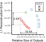
(a) DBLP

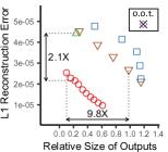
(b) Amazon-0302

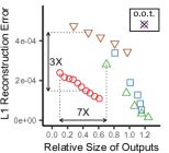
(c) Email-Enron

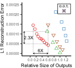
(d) Caida

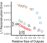
(e) Ego-Facebook

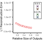
(f) Web-UK-05

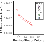
(g) Web-UK-02

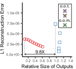
(h) LiveJournal

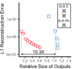
(i) Skitter

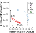
(j) Amazon-0601

Figure 4. SSumM yields compact and accurate summary graphs. o.o.t.: out of time (>12hours). o.o.m.: out of memory (>64GB). SSumM yielded up to $\mathbf{11.2\times}$ smaller summary graphs with similar reconstruction error. It also achieved up to $\mathbf{4.2\times}$ smaller reconstruction error with similarly concise outputs.

3.3. Complexity Analysis

We analyze the time and space complexities of SSumM. To this end, we define the neighborhood of a supernode $A\in S$ as $\bar{N}_{A}:=\{B\in S:\exists u\in A,~{}\exists v\in B\text{ s.t. }\{u,v\}\in E\}$, i.e., the set of supernodes that include a subnode adjacent to any subnode in $A$. For simplicity, we assume $|V|=O(|E|)$, as in most real-world graphs.

Time complexity: SSumM scales linearly with the size of the input graph, as formalized in Thm. 3.4, which is based on Lemma 3.3.

Lemma 3.3.

The merging and sparsification phase, i.e., lines 1-1 of Alg. 1, takes $O(|E|)$ time.

Proof.

Consider a candidate set $C\in\mathcal{S}_{t}$. Considering the termination condition (i.e., line 2 of Alg. 2), to merge a pair, $O(\log_{2}^{2}|C|+1)$ pairs are considered. Thus, finding the best pair among them takes $O((\log_{2}^{2}|C|+1)\cdot\max_{A\in C}|\bar{N}_{A}|)$ time, and if Eq. (20) is greater than $\theta(t)$, then merging the pair and sparsifying the adjacent superedges takes additional $O(\sum_{A\in C}|\bar{N}_{A}|)$ time. In total, a merger takes $O((\log_{2}^{2}|C|+1)\cdot\sum_{A\in C}|\bar{N}_{A}|)$ time, and since at most $|C|$ merges take place within $C$, the time complexity of processing a candidate set $C$ (i.e., Alg. 2) is $O(|C|\cdot(\log_{2}^{2}|C|+1)\cdot\sum_{A\in C}|\bar{N}_{A}|)$, which is $O(\sum_{A\in C}|\bar{N}_{A}|)$ because we upper bound $|C|$ by a constant, as described in Sect. 3.2.2. Since $\sum_{C\in\mathcal{S}_{t}}\sum_{A\in C}|\bar{N}_{A}|=\sum_{A\in S}|\bar{N}_{A}|\leq 2|E|$, processing all candidate sets in $\mathcal{S}_{t}$ takes $O(|E|)$ time. ∎

Theorem 3.4 (Linear Scalability of SSumM).

The time complexity of Alg. 1 is $O(T\cdot|E|)$.

Proof.

The initialization phase takes $O(1)$ time per subnode and subedge and thus $O(|V|+|E|)=O(|E|)$ time in total. The candidate generation and further sparsification phases take $O(|V|+|E|)=O(|E|)$ time, as discussed in Sects. 3.2.2 and 3.2.4. The merging and sparsification phase also takes $O(|E|)$ time, as proven in Lemma 3.3. Since each phase is repeated at most $T$ times, the total time complexity of Alg. 1 is $O(T\cdot|E|)$. ∎

Space complexity: SSumM (i.e., Alg. 1) needs to maintain (1) the input graph $G=(V,E)$, (2) the summary graph $\overline{G}=(S,P,\omega)$, (3) the neighborhood $\bar{N}_{A}$ of each supernode $A\in S$, and (4) a random hash function $h(v)$ for each subnode $v\in V$. Since $|S|\leq|V|$, $|P|\leq|E|$, and $\sum_{A\in S}|\bar{N}_{A}|\leq 2|E|$, its memory requirements are $O(|E|)$.

4. Experiments

We review our experiments designed for the following questions:

1. Compactness & Accuracy: Does SSumM yield more compact and accurate summary graphs than its best competitors?

2. Speed: Is SSumM faster than its best competitors?

3. Scalability: Does SSumM scale linearly with the size of the input graph? Can it handle graphs with about $1$ billion edges?

4. Effects of Parameters (Appendix A.2): How does the number of iterations $T$ affect the accuracy of summary graphs?

4.1. Experimental Settings

Machines: All experiments were conducted on a desktop with a 3.7 GHz Intel i5-9600k CPU and 64GB memory.

Datasets: We used the publicly available real-world graphs listed in Table 2 after removing all self-loops and the direction of all edges.

Implementations: We implemented SSumM and k-Gs (LeFevre and Terzi, 2010) in Java, and for S2L (Riondato et al., 2017) and SAA-Gs (Beg et al., 2018), we used the implementation in C++ and Java, resp., released by the authors. In SSumM The target summary size was set from 10% to 60% of the size of the input graph, at equal intervals. The number of iterations $T$ was fixed to $20$ unless otherwise stated (see Appendix A.2 for its effects.) For k-Gs, S2L, and SAA-Gs, the target number of supernodes was set from 10% to 60% of the number of nodes in the input graph, at equal intervals. For k-Gs, we used the SamplePairs method with $c=1.0$, as suggested in (LeFevre and Terzi, 2010). For SAA-Gs and SAA-Gs (linear sample), the number of sample pairs was set to $\log n$ and $n$, resp., and the count-min sketch was used with $w=50$ and $d=2$.

Table 2. Summary of the real-world datasets

Name	# Nodes	# Edges	Summary
Caida (CA) (Leskovec et al., 2005)	26,475	53,381	Internet
Ego-Facebook (EF) (Leskovec and Mcauley, 2012)	4,039	88,234	Social
Email-Enron (EE) (Klimt and Yang, 2004)	36,692	183,831	Email
Amazon-0302 (A3) (Leskovec et al., 2007)	262,111	899,792	Co-purchase
DBLP (DB) (Yang and Leskovec, 2015)	317,080	1,049,866	Collaboration
Amazon-0601 (A6) (Leskovec et al., 2007)	403,394	2,443,408	Co-purchase
Skitter (SK) (Leskovec et al., 2005)	1,696,415	11,095,298	Internet
LiveJournal (LJ) (Yang and Leskovec, 2015)	3,997,962	34,681,189	Social
Web-UK-02 (W2) (Boldi and Vigna, 2004)	18,483,186	261,787,258	Hyperlinks
Web-UK-05 (W5) (Boldi and Vigna, 2004)	39,454,463	783,027,125	Hyperlinks

Evaluation Metrics: We evaluated summary graphs in terms of accuracy, size, and quality. For accuracy, we measured $\ell_{1}$ and $\ell_{2}$ reconstruction errors, i.e., $RE_{1}$ and $RE_{2}$ (see Eq. (2)), and we normalized them by dividing them by the size of the adjacency matrix. For size, we used the number of bits required to store each summary graph (i.e., Eq. (4)). The quality of a summary graph is a metric for evaluating its accuracy and size at the same time. For quality, we (1) measured the reconstruction error $RE_{1}$ and size of the summary graphs obtained by all competitors, (2) normalized both so that they are between $0$ and $1$ in each dataset, and (3) computed $\sqrt{\text{normalized size}^{2}+\text{normalized reconstruction error}^{2}}$, i.e., the euclidean distance from the ideal quality. All evaluation metrics were averaged over $5$ iterations.

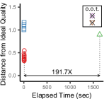
(a) DBLP

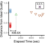
(b) Amazon-0302

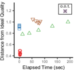
(c) Email-Enron

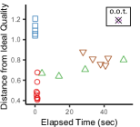
(d) Caida

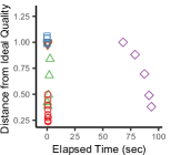
(e) Ego-Facebook

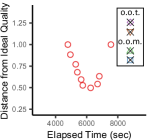
(f) Web-UK-05

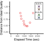
(g) Web-UK-02

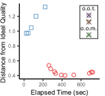
(h) LiveJournal

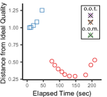
(i) Skitter

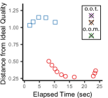
(j) Amazon-0601

Figure 5. SSumM is fast with high-quality summary graphs. o.o.t.: out of time (>12hours). o.o.m.: out of memory (>64GB). SSumM was up to $\mathbf{406.6\times}$ faster than the competitors with outputs of better quality. Only SSumM scaled to the largest datasets.

4.2. Q1. Compactness and Accuracy

We compared the size and $\ell_{1}$ reconstruction error ($RE_{1}$) of the summary graphs obtained by SSumM and its competitors. As seen in Fig. 4, SSumM yielded the most compact and accurate summaries in all the considered datasets. Specifically, SSumM gave a $\mathbf{11.2\times}$ smaller summary graph with similar or smaller $RE_{1}$ than its competitors in the Amazon-0601 dataset. It also gave a summary graph with $\mathbf{4.2\times}$ smaller $RE_{1}$ but similar or smaller sizes than its competitors in the Amazon-0601 dataset. We obtained consistent results when $RE_{2}$ was used instead of $RE_{1}$ (see Appendix A.1).

Note in Fig. 4 that competitors often gave summary graphs whose (relative) size is greater than $1$. That is, they failed to reduce the size in bits of the input graph since they focused solely on reducing the number of nodes. On the contrary, SSumM always gives a summary graph whose size does not exceed a given size in bits.

In Fig. 1, we visually compared the summary graphs obtained by different methods in the Ego-Facebook dataset. While they have similar $\ell_{1}$ reconstruction error (spec., $(5.9\pm{0.3})\times 10^{-3}$), one provided by SSumM is more concise with fewer edges.

4.3. Q2. Speed (Fig. 5)

We compared SSumM and its competitors in terms of speed and the quality of summary graphs. As seen in Fig. 5, SSumM gave the best trade-off between speed and the quality of the summary on all datasets. Specifically, SSumM was $\mathbf{406.6\times}$ faster than S2L while giving summary graphs with better quality in the Amazon-0302 dataset. While SAA-Gs was faster than SSumM, SSumM gave outputs of much higher quality than SAA-Gs. SAA-Gs (linear sample) and k-Gs were slower with lower-quality outputs than SSumM, and they did not scale to large datasets, taking more than $12$ hours.

4.4. Q3. Scalability (Fig. 6)

We evaluated the scalability of SSumM by measuring how its runtime changes depending on the size of the input graph. To this end, we used a number of graphs that are obtained from the Skitter and Livejournal datasets by randomly sampling different numbers of nodes. As seen in Fig. 6, SSumM scaled linearly with the size of the input graph, as formulated in Thm. 3.4. In addition, SSumM successfully processed $26\times$ larger datasets (with about $\mathbf{0.8}$ billion edges) than its best competitors, as seen Fig. 2(b).

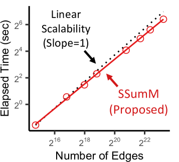
(a) Skitter

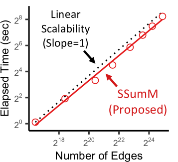
(b) Livejournal

Figure 6. SSumM is scalable. SSumM scaled linearly with the number of edges in the input graph.

5. Related Work

Graph summarization have been studied extensively for various objectives, including efficient queries (LeFevre and Terzi, 2010; Riondato et al., 2017; Tian et al., 2008), compression (Toivonen et al., 2011; Navlakha et al., 2008; Khan et al., 2014), and visualization (Dunne and Shneiderman, 2013; Koutra et al., 2014; Shen et al., 2006; Shah et al., 2015; Lin et al., 2008). See (Liu et al., 2018) for a survey. Below, we focus on previous studies directly related to Problem 1.

Given the target number of supernodes, k-Gs (LeFevre and Terzi, 2010) aims to minimize $\ell_{1}$ reconstruction error by repeatedly merging a pair of supernodes that decrease the $\ell_{1}$ reconstruction error most among candidate pairs. While several sampling methods are proposed to reduce the number of candidate pairs from $O(|V|^{2})$ to $O(|V|)$, k-Gs still takes $O(|V|^{3})$ time. Gs (LeFevre and Terzi, 2010) aims to minimize its loss function, which takes both reconstruction error and the number of supernodes into consideration. Gs greedily merges supernodes, as in k-Gs, until the loss function increases.

S2L (Riondato et al., 2017) uses geometric clustering for summarizing a graph with a given number of supernodes. Specifically, S2L considers each row (or column) in the adjacency matrix as a point in the $|V|$-dimensional space, and it employs $k$-means and $k$-median clustering to obtain clusters, each of which is considered as a supernode. It is shown that S2L provides a theoretical guarantee in terms of the $\ell_{p}$ reconstruction error of its output summary graph. To speed up clustering, which incurs expensive computation of the pairwise distances between many high-dimensional points, S2L also adopts dimensionality reduction (Indyk, 2006) and adaptive sampling (Aggarwal et al., 2009) techniques. The scalability of S2L is still limited due to high memory requirements for clustering and high time complexity. Its time complexity, $O(|E|+k|V|)$, becomes $O(|V|^{2})$ if $k=O(\lvert V\rvert)$.

SAA-Gs (Beg et al., 2018) is a more scalable algorithm for the same problem. Like k-Gs, SAA-Gs repeatedly merges the best supernode pair among some candidate pairs. When finding the candidate pairs, SAA-Gs uses a weighted sampling method designed to increase the probability that promising pairs are sampled. To speed up the candidate search, SAA-Gs maintains a tree storing the weights defined on each supernode, and it approximates reconstruction error using the count-min sketch (Cormode and Muthukrishnan, 2005). Although it has lower time complexity (spec., $O(|V|\log^{2}{|V|})$), the scalability of SAA-Gs is limited due to its high memory requirements for maintaining the tree.

Different from the aforementioned algorithms, which focus solely on reducing the number of supernodes by merging nodes, our proposed algorithm SSumM aims to minimize the size in bits of summary graphs by merging nodes and also sparsifying superedges.

A number of algorithms were developed for variants of the graph summarization problem (Toivonen et al., 2011; Navlakha et al., 2008; Shin et al., 2019; Ko et al., 2020; Khan et al., 2015; Koutra et al., 2014). As outputs, (Navlakha et al., 2008; Shin et al., 2019; Khan et al., 2015; Ko et al., 2020) yield an unweighted summary graph and edge corrections (i.e., edges to be added to or removed from the restored graph).

6. Conclusion

In this work, we consider a new practical variant of the graph summarization problem where the target size is given in bits rather than the number of nodes so that outputs easily fit target storage. Then, we propose SSumM, a fast and scalable algorithm for concise and accurate graph summarization. While balancing conciseness and accuracy, SSumM greedily combines two strategies: merging nodes and sparsifying edges. Moreover, SSumM achieves linear scalability by significantly but carefully reducing the search space without sacrificing the quality of outputs much. Throughout our extensive experiments on $10$ real-world graphs, we show that SSumM has the following advantages over its best competitors:

• Concise and Accurate: yields up to $\mathbf{11.2\times}$ more concise summary graphs with similar reconstruction error (Fig. 4).

• Fast: gives outputs of better quality up to $\mathbf{406.6\times}$ faster (Fig. 5).

• Scalable: summarizes graphs with about 0.8 billion edges (Fig. 2), scaling linearly with the size of the input graph (Thm. 3.4, Fig. 6).

Reproducibility: The source code and datasets used in the paper can be found at http://dmlab.kaist.ac.kr/ssumm/.

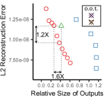
(a) DBLP

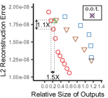
(b) Amazon-0302

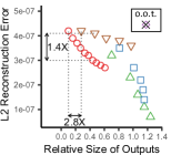
(c) Email-Enron

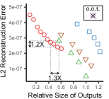
(d) Caida

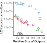
(e) Ego-Facebook

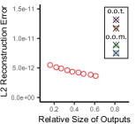
(f) Web-UK-05

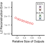
(g) Web-UK-02

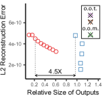
(h) LiveJournal

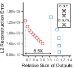
(i) Skitter

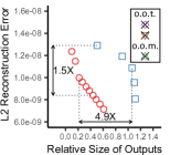
(j) Amazon-0601

Figure 7. SSumM yields compact and accurate summaries. o.o.t.: out of time (>12hours). o.o.m.: out of memory (>64GB). Specifically, SSumM yielded up to $\mathbf{8.5\times}$ smaller summary graphs with similar reconstruction error (spec., $RE_{2}$). It also achieved up to $\mathbf{1.5\times}$ smaller reconstruction error with similarly concise outputs.

Acknowledgements

This work was supported by National Research Foundation of Korea (NRF) grant funded by the Korea government (MSIT) (No. NRF-2019R1F1A1059755) and Institute of Information & Communications Technology Planning & Evaluation (IITP) grant funded by the Korea government (MSIT) (No. 2019-0-00075, Artificial Intelligence Graduate School Program (KAIST)).

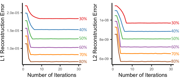
Figure 8. The effects of the iteration number $T$ in SSumM. Regardless of the target size, the reconstruction error of the output summary graph converged within $20$ iterations.

Appendix A Appendix: Extra Experiments

A.1. Compactness and Accuracy (Fig. 7)

We compared the size and $\ell_{2}$ reconstruction error ($RE_{2}$) of the summary graphs obtained by SSumM and its competitors in Fig. 7. As in Sect. 4.2, where $RE_{1}$ was used, SSumM consistently produced more concise and accurate summary graphs than its competitors.

A.2. Effects of Parameters (Fig. 8)

We measured how the number of iteration $T$ in SSumM affects the reconstruction error of its summary graph in the Amazon-0601 dataset by changing the target size of summary graph evenly from 30% to 80%. As seen in Fig. 8, the reconstruction error decreased over iterations and eventually converged. As the target size decreased, more iterations were needed for convergence. In all settings, however, $20$ iterations were enough for convergence.

Appendix B Appendix: Proofs

In this section, we provide proofs of Lemmas 3.1 and 3.2 in Sect. 3.2.2. The proofs are based on Lemmas B.1 and B.2.

Lemma B.1.

If two supernodes $A\neq B\in S$ are merged into a single supernode $A^{\prime}:=A\cup B$, then

(24) $$Cost^{\star}_{AC}(S)\leq Cost^{\star}_{A^{\prime}C}(S^{\prime}),\;\;\;\forall C\in S\setminus\{A,B\},$$

where $S^{\prime}:=S\cup\{A^{\prime}\}\setminus\{A,B\}$.

Proof.

Let $\bar{C}:=2\log_{2}|V|+\log_{2}|E|$. From Eqs. (11), (12), (15),

$$Cost^{\star}_{A^{\prime}C}(S^{\prime})=\left\{\begin{array}[]{ll}\bar{C}+Cost_{(1)}(E_{A^{\prime}C}|\bar{G}^{\star}(S^{\prime}))&\text{if}~{}\{A^{\prime},C\}\in P^{\star}(S^{\prime})\\ Cost_{(2)}(E_{A^{\prime}C}|\bar{G}^{\star}(S^{\prime}))&\text{otherwise}.\\ \end{array}\right.$$

We show that Eq. (24) holds by dividing into $4$ cases as follows:

1. Case 1. $\{A,C\}\notin P^{\star}(S)$ and $\{A^{\prime},C\}\notin P^{\star}(S^{\prime})$:

   $$Cost^{\star}_{AC}(S)=Cost_{(2)}(E_{AC}|\bar{G}^{\star}(S))=2|E_{AC}|\log_{2}|V|$$

   (25) $$~{}~{}\leq 2|E_{A^{\prime}C}|\log_{2}|V|=Cost_{(2)}(E_{A^{\prime}C}|\bar{G}^{\star}(S^{\prime}))=Cost^{\star}_{A^{\prime}C}(S^{\prime}).$$

2. Case 2. $\{A,C\}\in P^{\star}(S)$ and $\{A^{\prime},C\}\in P^{\star}(S^{\prime})$:
   Let $\sigma_{AC}:=\frac{|E_{AC}|}{|\Pi_{AC}|}$ and $\sigma_{A^{\prime}C}:=\frac{|E_{A^{\prime}C}|}{|\Pi_{A^{\prime}C}|}$. Then,

   $$Cost^{\star}_{AC}(S)=\bar{C}+Cost_{(1)}(E_{AC}|\bar{G}^{\star}(S))$$

   $$~{}~{}=\bar{C}-|\Pi_{AC}|(\sigma_{AC}\log_{2}\sigma_{AC}+(1-\sigma_{AC})\log_{2}(1-\sigma_{AC}))$$

   $$~{}~{}\leq\bar{C}-|\Pi_{AC}|(\sigma_{A^{\prime}C}\log_{2}\sigma_{A^{\prime}C}+(1-\sigma_{A^{\prime}C})\log_{2}(1-\sigma_{A^{\prime}C}))$$

   $$~{}~{}\leq\bar{C}-|\Pi_{A^{\prime}C}|(\sigma_{A^{\prime}C}\log_{2}\sigma_{A^{\prime}C}+(1-\sigma_{A^{\prime}C})\log_{2}(1-\sigma_{A^{\prime}C}))$$

   (26) $$~{}~{}=\bar{C}+Cost_{(1)}(E_{A^{\prime}C}|\bar{G}^{\star}(S))=Cost^{\star}_{A^{\prime}C}(S^{\prime}),$$

   where the first inequality holds by Shannon’s source coding theorem (Shannon and Weaver, 1998).

3. Case 3. $\{A,C\}\notin P^{\star}(S)$ and $\{A^{\prime},C\}\in P^{\star}(S^{\prime})$:

   $$Cost^{\star}_{AC}(S)=Cost_{(2)}(E_{AC}|\bar{G}^{\star}(S))\leq\bar{C}+Cost_{(1)}(E_{AC}|\bar{G}^{\star}(S))$$

   $$~{}~{}\leq\bar{C}+Cost_{(1)}(E_{A^{\prime}C}|\bar{G}^{\star}(S))=Cost^{\star}_{A^{\prime}C}(S^{\prime}),$$

   where the first inequality holds from the optimality of $P^{\star}(S)$, and the second one can be shown as exactly in Eq. (26).

4. Case 4. $\{A,C\}\in P^{\star}(S)$ and $\{A^{\prime},C\}\notin P^{\star}(S^{\prime})$:

   $$Cost^{\star}_{AC}(S)=\bar{C}+Cost_{(1)}(E_{AC}|\bar{G}^{\star}(S))\leq Cost_{(2)}(E_{AC}|\bar{G}^{\star}(S))$$

   $$~{}~{}\leq Cost_{(2)}(E_{A^{\prime}C}|\bar{G}^{\star}(S))=Cost^{\star}_{A^{\prime}C}(S^{\prime}),$$

   where the first inequality holds from the optimality of $P^{\star}(S)$, and the second one can be shown as exactly in Eq. (25). ∎

Lemma B.2.

If two supernodes $A\neq B\in S$ are merged into a single supernode $A^{\prime}:=A\cup B$, then the following inequalities hold:

1. $~{}~{}Cost_{(1)}(E_{AA}|\bar{G}^{\star}(S))+Cost_{(1)}(E_{BB}|\bar{G}^{\star}(S))$

   (27) $$\qquad\leq Cost_{(1)}(E_{A^{\prime}A^{\prime}}|\bar{G}^{\star}(S^{\prime})),$$

2. $~{}~{}Cost_{(2)}(E_{AA}|\bar{G}^{\star}(S))+Cost_{(2)}(E_{BB}|\bar{G}^{\star}(S))$

   (28) $$\qquad\leq Cost_{(2)}(E_{A^{\prime}A^{\prime}}|\bar{G}^{\star}(S^{\prime})),$$

3. (29) $$Cost^{\star}_{AA}(S)+Cost^{\star}_{BB}(S)\leq\bar{C}+Cost^{\star}_{A^{\prime}A^{\prime}}(S^{\prime}),\qquad\quad\$$

4. (30) $$Cost^{\star}_{AA}(S)\leq Cost^{\star}_{A^{\prime}A^{\prime}}(S^{\prime}),\qquad\qquad\qquad\qquad\quad\quad$$

where $S^{\prime}:=S\cup\{A^{\prime}\}\setminus\{A,B\}$.

Proof.

Let $\bar{C}:=2\log_{2}|V|+\log_{2}|E|$. From Eqs. (11), (12), (15),

(31) $$Cost^{\star}_{A^{\prime}A^{\prime}}(S^{\prime})=\left\{\begin{array}[]{ll}\bar{C}+Cost_{(1)}(E_{A^{\prime}A^{\prime}}|\bar{G}^{\star}(S^{\prime}))&\text{if}~{}\{A^{\prime},A^{\prime}\}\in P^{\star}(S^{\prime})\\ Cost_{(2)}(E_{A^{\prime}A^{\prime}}|\bar{G}^{\star}(S^{\prime}))&\text{otherwise}.\end{array}\right.$$

First, we show Eq. (27) holds. Let $\sigma_{A^{\prime}A^{\prime}}:=\frac{|E_{A^{\prime}A^{\prime}}|}{|\Pi_{A^{\prime}A^{\prime}}|}$. Then, Eq. (9) and Shannon’s source coding theorem (Shannon and Weaver, 1998) imply

$$Cost_{(1)}(E_{AA}|\bar{G}^{\star}(S))+Cost_{(1)}(E_{BB}|\bar{G}^{\star}(S))$$

$$\leq-(|\Pi_{AA}|+|\Pi_{AB}|)\cdot(\sigma_{A^{\prime}A^{\prime}}\log_{2}\sigma_{A^{\prime}A^{\prime}}+(1-\sigma_{A^{\prime}A^{\prime}})\log_{2}(1-\sigma_{A^{\prime}A^{\prime}}))$$

$$\leq-|\Pi_{A^{\prime}A^{\prime}}|(\sigma_{A^{\prime}A^{\prime}}\log_{2}\sigma_{A^{\prime}A^{\prime}}+(1-\sigma_{A^{\prime}A^{\prime}})\log_{2}(1-\sigma_{A^{\prime}A^{\prime}}))$$

$$=Cost_{(1)}(E_{A^{\prime}A^{\prime}}|\bar{G}^{\star}(S^{\prime})),$$

Second, we show Eq. (28) holds. Eq. (9) and $|E_{AA}|+|E_{BB}|\leq|E_{A^{\prime}A^{\prime}}|$ imply

$$Cost_{(2)}(E_{AA}|\bar{G}^{\star}(S))+Cost_{(2)}(E_{BB}|\bar{G}^{\star}(S))$$

$$=2*(|E_{AA}|+|E_{BB}|)\log_{2}|V|\leq 2*|E_{A^{\prime}A^{\prime}}|\log_{2}|V|\qquad\qquad\qquad$$

$$=Cost_{(2)}(E_{A^{\prime}A^{\prime}}|\bar{G}^{\star}(S^{\prime})).$$

Third, we show Eq. (29) holds. The optimality of $P^{\star}(S)$ and Eqs. (27) and (28) imply

$$Cost^{\star}_{AA}(S) +Cost^{\star}_{BB}(S)$$

$$\leq 2\bar{C}+Cost_{(1)}(E_{AA}|\bar{G}^{\star}(S))+Cost_{(1)}(E_{BB}|\bar{G}^{\star}(S))\qquad\$$

(32) $$\leq 2\bar{C}+Cost_{(1)}(E_{A^{\prime}A^{\prime}}|\bar{G}^{\star}(S^{\prime}))$$

$$Cost^{\star}_{AA}(S) +Cost^{\star}_{BB}(S)$$

$$\leq Cost_{(2)}(E_{AA}|\bar{G}^{\star}(S))+Cost_{(2)}(E_{BB}|\bar{G}^{\star}(S))\qquad\qquad\quad$$

(33) $$\leq Cost_{(2)}(E_{A^{\prime}A^{\prime}}|\bar{G}^{\star}(S^{\prime})).$$

The optimality of $P^{\star}(S^{\prime})$ and Eqs. (32) and (33) imply

$$Cost^{\star}_{AA}(S) +Cost^{\star}_{BB}(S)$$

$$\leq\min(2\bar{C}+Cost_{(1)}(E_{A^{\prime}A^{\prime}}|\bar{G}^{\star}(S^{\prime})),Cost_{(2)}(E_{A^{\prime}A^{\prime}}|\bar{G}^{\star}(S^{\prime})))$$

$$\leq\bar{C}+Cost^{\star}_{A^{\prime}A^{\prime}}(S^{\prime}).$$

Lastly, we show Eq. (30) holds. The optimality of $P^{\star}(S)$ and Eqs. (27) and (28) imply

$$Cost^{\star}_{AA}(S) \leq\bar{C}+Cost_{(1)}(E_{AA}|\bar{G}^{\star}(S))$$

(34) $$\leq\bar{C}+Cost_{(1)}(E_{A^{\prime}A^{\prime}}|\bar{G}^{\star}(S^{\prime})),$$

$$Cost^{\star}_{AA}(S) \leq Cost_{(2)}(E_{AA}|\bar{G}^{\star}(S))\quad\quad\ \ \$$

(35) $$\leq Cost_{(2)}(E_{A^{\prime}A^{\prime}}|\bar{G}^{\star}(S^{\prime})).$$

The optimality of $P^{\star}(S^{\prime})$ and Eqs. (31), (34), and (35) imply

$$Cost^{\star}_{AA}(S)$$

$$~{}~{}~{}\leq\min(\bar{C}+Cost_{(1)}(E_{A^{\prime}A^{\prime}}|\bar{G}^{\star}(S^{\prime})),Cost_{(2)}(E_{A^{\prime}A^{\prime}}|\bar{G}^{\star}(S^{\prime})))$$

$$~{}~{}~{}\leq Cost^{\star}_{A^{\prime}A^{\prime}}(S^{\prime}).\qed$$

B.1. Proof of Lemma 3.1

Proof.

Suppose two $A\neq B\in S$ that are within $2$ hops are merged into a single supernode $A^{\prime}:=A\cup B$, and without loss of generality, $Cost^{\star}_{A}(S)\geq Cost^{\star}_{B}(S)$. We let $S^{\prime}:=S\cup\{A^{\prime}\}\setminus\{A,B\}$.

We first show that Eq. (18) holds. From Eqs. (24) and (30),

$$Cost^{\star}_{A}(S)-Cost^{\star}_{AB}(S)=Cost^{\star}_{AA}(S)+\sum\nolimits_{C\in S\setminus\{A,B\}}Cost^{\star}_{AC}(S)$$

(36) $$\leq Cost^{\star}_{A^{\prime}A^{\prime}}(S^{\prime})+\sum\nolimits_{C\in S\setminus\{A,B\}}Cost^{\star}_{A^{\prime}C}(S^{\prime})=Cost^{\star}_{A^{\prime}}(S^{\prime}).$$

Eq. (17), Eq. (36), and $Cost^{\star}_{A}(S)\geq Cost^{\star}_{B}(S)$ imply Eq. (18).

Now, we show that Eq. (18) is tight. That is, we show that there exists $A\neq B\in S$ within $2$ hops where

(37) $$Reduction(A,B)=\min(Cost^{\star}_{A}(S),Cost^{\star}_{B}(S)).$$

Fig. 9, where $A$ and $B$ are 2 hops away from each other, provides such an example. In the example,

$$Cost^{\star}_{A}(S)=Cost^{\star}_{B}(S)=2\cdot(2\log_{2}|V|+\log_{2}|E|)=Cost^{\star}_{A^{\prime}A^{\prime}}(S^{\prime}),$$

and $Cost^{\star}_{AB}(S)=0$. Hence,

$$Reduction(A,B) =2\cdot(2\log_{2}|V|+\log_{2}|E|)$$

$$=\min(Cost^{\star}_{A}(S),Cost^{\star}_{B}(S)).\qed$$

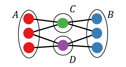
Figure 9. An example pair of supernodes $\boldsymbol{\{A,B\}}$ which are $\boldsymbol{2}$ hops away from each other.

B.2. Proof of Lemma 3.2

Proof.

Suppose two supernodes $A\neq B\in S$ that are $3$ or more hops away from each other are merged into a single supernode $A^{\prime}:=A\cup B$. Then, the following equalities hold:

(38) $$Cost^{\star}_{AB}(S)=0,$$

(39) $$Cost^{\star}_{AC}(S)=0\;\;or\;\;Cost^{\star}_{BC}(S)=0,\;\;\;\forall C\in S\setminus\{A,B\}.$$

Eqs. (24), (38), and (39) imply

(40) $$Cost^{\star}_{AC}(S)+Cost^{\star}_{BC}(S)\leq Cost^{\star}_{A^{\prime}C}(S^{\prime}),\;\;\;\forall C\in S\setminus\{A,B\},$$

where $S^{\prime}:=S\cup\{A^{\prime}\}\setminus\{A,B\}$. Then, Eqs. (29), (38) and (40) imply

$$Cost^{\star}_{A}(S) +Cost^{\star}_{B}(S)-Cost^{\star}_{AB}(S)$$

$$=Cost^{\star}_{AA}(S)+Cost^{\star}_{BB}(S)+Cost^{\star}_{AB}(S)$$

$$\quad+\sum\nolimits_{C\in S\setminus\{A,B\}}(Cost^{\star}_{AC}(S)+Cost^{\star}_{BC}(S))$$

$$\leq\bar{C}+Cost^{\star}_{A^{\prime}A^{\prime}}(S^{\prime})+\sum\nolimits_{C\in S\setminus\{A,B\}}Cost^{\star}_{A^{\prime}C}(S^{\prime})$$

(41) $$=\bar{C}+Cost^{\star}_{A^{\prime}}(S^{\prime}),$$

where $\bar{C}:=2\log_{2}|V|+\log_{2}|E|$. Eqs. (41) and (17) imply Eq. (19). ∎

References

- (1)
- Aggarwal et al. (2009) Ankit Aggarwal, Amit Deshpande, and Ravi Kannan. 2009. Adaptive sampling for k-means clustering. In Approximation, Randomization, and Combinatorial Optimization. Algorithms and Techniques. Springer, 15–28.
- Apostolico and Drovandi (2009) Alberto Apostolico and Guido Drovandi. 2009. Graph compression by BFS. Algorithms 2, 3 (2009), 1031–1044.
- Beg et al. (2018) Maham Anwar Beg, Muhammad Ahmad, Arif Zaman, and Imdadullah Khan. 2018. Scalable approximation algorithm for graph summarization. In PAKDD.
- Blum et al. (1973) Manuel Blum, Robert W. Floyd, Vaughan R. Pratt, Ronald L. Rivest, and Robert Endre Tarjan. 1973. Time bounds for selection. JCSS 7, 4 (1973), 448–461.
- Boldi and Vigna (2004) Paolo Boldi and Sebastiano Vigna. 2004. The webgraph framework I: compression techniques. In WWW.
- Buehrer and Chellapilla (2008) Gregory Buehrer and Kumar Chellapilla. 2008. A scalable pattern mining approach to web graph compression with communities. In WSDM.
- Chierichetti et al. (2009) Flavio Chierichetti, Ravi Kumar, Silvio Lattanzi, Michael Mitzenmacher, Alessandro Panconesi, and Prabhakar Raghavan. 2009. On compressing social networks. In KDD.
- Ching et al. (2015) Avery Ching, Sergey Edunov, Maja Kabiljo, Dionysios Logothetis, and Sambavi Muthukrishnan. 2015. One trillion edges: graph processing at Facebook-scale. PVLDB 8, 12 (2015), 1804–1815.
- Cormode and Muthukrishnan (2005) Graham Cormode and Shan Muthukrishnan. 2005. An improved data stream summary: the count-min sketch and its applications. Journal of Algorithms 55, 1 (2005), 58–75.
- Dunne and Shneiderman (2013) Cody Dunne and Ben Shneiderman. 2013. Motif simplification: improving network visualization readability with fan, connector, and clique glyphs. In SIGCHI.
- Indyk (2006) Piotr Indyk. 2006. Stable distributions, pseudorandom generators, embeddings, and data stream computation. JACM 53, 3 (2006), 307–323.
- Khan et al. (2014) Kifayat Ullah Khan, Waqas Nawaz, and Young-Koo Lee. 2014. Set-based unified approach for attributed graph summarization. In CBDCom.
- Khan et al. (2015) Kifayat Ullah Khan, Waqas Nawaz, and Young-Koo Lee. 2015. Set-based approximate approach for lossless graph summarization. Computing 97, 12 (2015), 1185–1207.
- Kirkpatrick et al. (1983) Scott Kirkpatrick, C Daniel Gelatt, and Mario P Vecchi. 1983. Optimization by simulated annealing. Science 220, 4598 (1983), 671–680.
- Klimt and Yang (2004) Bryan Klimt and Yiming Yang. 2004. Introducing the Enron corpus. In CEAS.
- Knuth (1969) DE Knuth. 1969. Seminymerical Algorithms. The Art of Computer Programming, Vol. 2.
- Ko et al. (2020) Jihoon Ko, Yunbum Kook, and Kijung Shin. 2020. Incremental Lossless Graph Summarization. In KDD.
- Koutra et al. (2014) Danai Koutra, U Kang, Jilles Vreeken, and Christos Faloutsos. 2014. VoG: Summarizing and understanding large graphs. In SDM.
- LeFevre and Terzi (2010) Kristen LeFevre and Evimaria Terzi. 2010. GraSS: Graph structure summarization. In SDM.
- Leskovec et al. (2007) Jure Leskovec, Lada A Adamic, and Bernardo A Huberman. 2007. The dynamics of viral marketing. TWEB 1, 1 (2007), 5.
- Leskovec et al. (2005) Jure Leskovec, Jon Kleinberg, and Christos Faloutsos. 2005. Graphs over time: densification laws, shrinking diameters and possible explanations. In KDD.
- Leskovec and Mcauley (2012) Jure Leskovec and Julian J Mcauley. 2012. Learning to discover social circles in ego networks. In NIPS.
- Lin et al. (2008) Yu Ru Lin, Hari Sundaram, and Aisling Kelliher. 2008. Summarization of social activity over time: People, actions and concepts in dynamic networks. In CIKM.
- Liu et al. (2018) Yike Liu, Tara Safavi, Abhilash Dighe, and Danai Koutra. 2018. Graph summarization methods and applications: A survey. CSUR 51, 3 (2018), 62.
- Meusel et al. (2015) Robert Meusel, Sebastiano Vigna, Oliver Lehmberg, and Christian Bizer. 2015. The Graph Structure in the Web - Analyzed on Different Aggregation Levels. The Journal of Web Science 1, 1 (2015), 33–47.
- Navlakha et al. (2008) Saket Navlakha, Rajeev Rastogi, and Nisheeth Shrivastava. 2008. Graph summarization with bounded error. In SIGMOD.
- Page et al. (1999) Lawrence Page, Sergey Brin, Rajeev Motwani, and Terry Winograd. 1999. The PageRank citation ranking: Bringing order to the web. Technical Report. Stanford InfoLab.
- Riondato et al. (2017) Matteo Riondato, David García-Soriano, and Francesco Bonchi. 2017. Graph summarization with quality guarantees. DMKD 31, 2 (2017), 314–349.
- Rissanen (1978) Jorma Rissanen. 1978. Modeling by shortest data description. Automatica 14, 5 (1978), 465–471.
- Shah et al. (2015) Neil Shah, Danai Koutra, Tianmin Zou, Brian Gallagher, and Christos Faloutsos. 2015. Timecrunch: Interpretable dynamic graph summarization. In KDD.
- Shannon and Weaver (1998) Claude E Shannon and Warren Weaver. 1998. The mathematical theory of communication. University of Illinois Press.
- Shen et al. (2006) Zeqian Shen, Kwan-Liu Ma, and Tina Eliassi-Rad. 2006. Visual analysis of large heterogeneous social networks by semantic and structural abstraction. IEEE TVCG 12, 6 (2006), 1427–1439.
- Shin et al. (2019) Kijung Shin, Amol Ghoting, Myunghwan Kim, and Hema Raghavan. 2019. SWeG: Lossless and lossy summarization of web-scale graphs. In WWW.
- Tian et al. (2008) Yuanyuan Tian, Richard A. Hankins, and Jignesh M. Patel. 2008. Efficient aggregation for graph summarization. In SIGMOD.
- Toivonen et al. (2011) Hannu Toivonen, Fang Zhou, Aleksi Hartikainen, and Atte Hinkka. 2011. Compression of weighted graphs. In KDD.
- Tsourakakis (2015) Charalampos Tsourakakis. 2015. The k-clique densest subgraph problem. In WWW.
- Yang and Leskovec (2015) Jaewon Yang and Jure Leskovec. 2015. Defining and evaluating network communities based on ground-truth. KAIS 42, 1 (2015), 181–213.