Bootstrap inference for quantile-based modal regression
Abstract
In this paper, we develop uniform inference methods for the conditional mode based on quantile regression. Specifically, we propose to estimate the conditional mode by minimizing the derivative of the estimated conditional quantile function defined by smoothing the linear quantile regression estimator, and develop two bootstrap methods, a novel pivotal bootstrap and the nonparametric bootstrap, for our conditional mode estimator. Building on high-dimensional Gaussian approximation techniques, we establish the validity of simultaneous confidence rectangles constructed from the two bootstrap methods for the conditional mode. We also extend the preceding analysis to the case where the dimension of the covariate vector is increasing with the sample size. Finally, we conduct simulation experiments and a real data analysis using U.S. wage data to demonstrate the finite sample performance of our inference method. The supplemental materials include the wage dataset, R codes and an appendix containing proofs of the main results, additional simulation results, discussion of model misspecification and quantile crossing, and additional details of the numerical implementation.
Keywords: quantile regression, kernel smoothing, modal regression, high-dimensional CLT, pivotal bootstrap
1 Introduction
1.1 Overview
Modal regression is a principal statistical methodology to estimate and make inference on the conditional mode. Modes provide useful distributional information missed by the mean when the (conditional) distribution is skewed (Chen et al.,, 2016) and are known to be robust under measurement errors (Bound and Krueger, 1991; Hu and Schennach, 2008). The global mode offers intuitive interpretability by being understood as “the most likely” or “the most common” (Heckman et al., 2001; Hedges and Shah, 2003). As such, modal regression has wide applications in various areas including astronomy (Bamford et al.,, 2008), medical research (Wang et al.,, 2017), econometrics (Kemp and Santos-Silva,, 2012), etc. We refer the reader to Chacón, (2018) and Chen, (2018) for recent reviews on modal regression; see also a literature review below.
In this paper, we consider estimating the conditional mode by “inverting” a quantile regression model, which builds on the observation that the derivative of the conditional quantile function coincides with the reciprocal of the conditional density so that the conditional mode can be obtained by minimizing the derivative of the conditional quantile function. Specifically, we estimate the conditional mode by minimizing the derivative of the kernel smoothed Koenker-Bassett estimator of the conditional quantile function (Koenker and Bassett,, 1978) with a sufficiently smooth kernel. We develop asymptotic theory for the proposed estimator of the conditional mode . In particular, we consider simultaneous confidence intervals for the conditional mode at multiple design points, , where is allowed to grow with the sample size , i.e., . To this end, we first show that can be approximated by the linear term uniformly over a range of design points , where is a sequence of bandwidths, is the influence function (that depends on ) at design point , are independent covariate vectors, and are mutually independent uniform random variables on independent of the covariate vectors. Building on high dimensional Gaussian approximation techniques developed in Chernozhukov et al., (2014); Chernozhukov et al., 2017a , we show that can be approximated by an -dimensional Gaussian vector uniformly over the hyperrectangles in , i.e., all sets of the form: for some , , even when .
As the limiting Gaussian distribution is infeasible in practice, we consider two bootstrap methods, the nonparametric bootstrap and a novel pivotal bootstrap, to conduct valid inference. We first discuss the motivation of the new pivotal bootstrap. The leading stochastic term in the prescribed expansion is conditionally “pivotal” in the sense that conditionally on , the distribution of the process
is completely known up to some nuisance parameters. This suggests a version of bootstrap for the proposed estimator by sampling uniform random variables independent of the data. In practice, the influence function depends on nuisance parameters and we replace them by consistent estimates. We call the resulting bootstrap “pivotal bootstrap” and prove that the pivotal bootstrap can consistently estimate the sampling distribution of uniformly over the rectangles in even when . In fact, our inference framework is more general and covers simultaneous inference for linear combinations of the vector , which can be used to construct simultaneous confidence intervals for partial effects and test significance of certain covariates on the conditional mode. We also establish a similar consistency result for the nonparametric bootstrap. Finally, we extend the previous analysis to the case where the dimension of the covariate vector increases with the sample size.
We conduct simulation experiments on various mode inference problems and a real data analysis to demonstrate the finite sample performance of the bootstrap methods. Our simulation experiments show that the pivotal bootstrap yields accurate pointwise and simultaneous confidence intervals for the conditional modes. Additionally, we apply our inference method to analyze a real U.S. wage dataset. Analysis of wage data is important in econometric and social science (Autor et al., 2008; Western and Rosenfeld, 2011; Buchinsky, 1994). Wage data are often positively skewed and “the most common wage” as a representative of the majority of the population is usually of more interest. Common questions in the analysis of wage data include: i) What is the most likely wage for given covariates? How to construct pointwise and simultaneous confidence intervals for the estimated wages? ii) Is there an effect of a specific covariate on the most likely wage given the same other covariates? We address those empirical questions using the inference method developed in the present paper.
From a technical perspective, the asymptotic analysis in this paper is highly nontrivial. Our program of the technical analysis proceeds as 1) first establishing a uniform asymptotic representation and 2) high-dimensional Gaussian approximation to our estimate, and 3) then proving the validity of the pivotal and nonparametric bootstraps building on 1) and 2). Each of these steps relies on modern empirical process theory and high-dimensional Gaussian approximation techniques recently developed by Chernozhukov et al., (2014); Chernozhukov et al., 2017a . In particular, the pivotal bootstrap differs from the nonparametric or multiplier bootstraps that have been analyzed in the literature in the high-dimensional setup (Belloni et al.,, 2019; Chernozhukov et al.,, 2016; Deng and Zhang,, 2017; Chen and Kato,, 2020), and proving the validity of the pivotal bootstrap requires a substantial work. Further, we employ a new multiplier inequality for the empirical process in Han and Wellner, (2019) to establish the validity of the nonparametric bootstrap.
In summary, the present paper contributes to the literature on modal regression in twofold. First, we propose a new quantile-based conditional mode estimate that enjoys both desirable computational and statistical guarantees. The proposed estimator only requires solving a linear quantile regression problem and a one-dimensional optimization both of which can be solved efficiently. Second, we establish the theoretical validity of two bootstrap methods for a broad spectrum of inference tasks in a unified way. In particular, we propose a new resampling method (pivotal bootstrap) that builds on an insight into the specific structure of our estimate.
1.2 Literature review
Starting from the pioneering work of Sager and Thisted, (1982), there is now a large literature on modal regression. There are two major approaches to estimating the conditional mode comparable to our method; one is linear modal regression where the conditional mode is assumed to be linear in covariates (Lee,, 1989, 1993; Kemp and Santos-Silva,, 2012; Yao and Li,, 2014), and the other is nonparametric estimation (Yao et al.,, 2012; Chen et al.,, 2016; Yao and Xiang,, 2016; Feng et al.,, 2020); see also Lee and Kim, (1998); Manski, (1991); Einbeck and Tutz, (2006); Sasaki et al., (2016); Ho et al., (2017); Khardani and Yao, (2017); Krief, (2017) for alternative methods including semiparametric and Bayesian estimation. Lee, (1989, 1993) assume symmetry of the error distribution to derive limit theorems for their proposed estimators, but the symmetry assumption implies that the conditional mean, median, and mode coincide, thereby significantly reducing the complexity of estimating the conditional mode. Kemp and Santos-Silva, (2012) and Yao and Li, (2014) consider an alternative estimator defined by minimizing a kernel-based loss function for linear modal regression and develop limit distribution theory for the estimator without assuming symmetry of the error distribution. However, the optimization problem of Kemp and Santos-Silva, (2012) and Yao and Li, (2014) is (multidimensional and) nonconvex, and while they propose EM-type algorithms to compute their estimators, “there is no guarantee that the algorithm will converge to the global optimal solution” (Yao and Li,, 2014, p. 659). Compared with the method of Kemp and Santos-Silva, (2012) and Yao and Li, (2014), all three methods (including ours) enjoy the same rate of convergence, while our method is computationally attractive since linear quantile regression can be formulated as a linear programming problem (Koenker,, 2005), and minimizing the estimated derivative of the conditional quantile function is a one-dimensional optimization problem both of which can be solved accurately and efficiently.
Yao et al., (2012) consider local linear estimation of the conditional mode but their Condition (A6) is essentially the symmetry assumption on the error distribution, which makes their problem statistically equivalent to conditional mean estimation. Chen et al., (2016) study nonparametric estimation of the conditional mode based on kernel density estimation (KDE), and develop nonparametric bootstrap inference for their KDE-based estimate. The nonparametric estimation is able to avoid model misspecification. Chen et al., (2016) also allow for multiple local modes, while we assume the existence of the unique global mode at each design point of interest. Thus, the setup of Chen et al., (2016) is more general than ours. However, the convergence rate of the KDE-based estimate of Chen et al., (2016) is slow even when the dimension of the covariate vector is moderately large (“curse of dimensionality”). Specifically, the convergence rate of the Chen et al., (2016) estimate is at best where is the number of continuous covariates under the assumption of four times differentiability of the conditional density, while our estimate can achieve the rate (up to logarithmic factors when evaluated under the uniform norm) assuming three times differentiability of the conditional density (albeit assuming a linear quantile regression model). Finally, Chen et al., (2016) also consider the application of the nonparametric bootstrap to inference on the conditional mode. However, our estimator is substantially different from their estimator and requires different analysis to establish the validity of the nonparametric bootstrap.
The present paper builds on (but substantially differs from) the recent work of Ota et al., (2019), which proposes a different quantile-based estimate of the conditional mode and develops pointwise limit distribution theory for their estimator. Contrary to ours, Ota et al., (2019) directly use the linear quantile regression estimate and minimize its difference quotient (as the linear quantile regression estimate is not smooth in the quantile index), which makes a substantial difference between their asymptotic analysis and ours. Indeed, Ota et al., (2019) show that the rate of convergence of their estimate is at best that is slower than our rate, and find that the pointwise limit distribution is a scale transformation of nonstandard Chernoff’s distribution. The nonstandard limit distribution poses a substantial challenge in inference using their estimate and Ota et al., (2019) only consider pointwise inference using a general purpose subsampling method (Politis et al.,, 1999). We overcome this limitation by employing kernel smoothing, and further, develop a model-based bootstrap method (pivotal bootstrap) that enables us to deal with much broader inference tasks including simultaneous confidence intervals and significance testing.
This paper also builds on and contributes to the quantile regression literature. Quantile regression provides a comparatively full picture of how the covariates impact the conditional distribution of a response variable and has wide applications (Koenker,, 2017). In particular, the pivotal bootstrap of the present paper is related to Parzen et al., (1994); Chernozhukov et al., (2009); He, (2017); Belloni et al., (2019) who study resampling-based inference methods that build on (conditionally) pivotal influence functions in the quantile regression setup. Their scopes and methods are, however, substantially different from ours. To the best of our knowledge, exploiting pivotal influence functions to make inference for modal regression is new.
1.3 Organization
The rest of the paper is organized as follows. In Section 2, we introduce the setup and define the proposed quantile-based modal estimator. In Section 3, we present the main theoretical results for the proposed estimator. We first derive a uniform asymptotic linear representation for the proposed estimator. Then we present our general inference framework based on the pivotal and nonparametric bootstraps together with their theoretical guarantees. In Section 4, we present the simulation results and a real data example. In Section 5, we extend the preceding analysis to the increasing dimension case. Finally, we summarize the paper in Section 6. The proofs of main results and additional discussion are relegated to the Appendix which is included in the supplemental materials.
2 Mode estimation via smoothed quantile regression
We begin with the setup and define our estimator. We are interested in making inference on the conditional mode of a scalar response variable given a -dimensional covariate vector . We will initially assume that the dimension is fixed in Section 3, but consider the extension to the case with in Section 5. In what follows, we assume that there exists a conditional density of given , , which is (at least) continuous in for each design point . We are interested in making inference on the conditional mode over a compact subset of the support of . We assume that for each , there exists a unique global mode , i.e., is the unique maximizer of the function ,
| (1) |
Our strategy to estimate the conditional mode is based on “inverting” a quantile regression model. For , let denote the conditional -quantile of given . Observe that the derivative of the conditional quantile function with respect to the quantile index coincides with the reciprocal of the conditional density at , i.e.,
| (2) |
This suggests that the conditional mode can be obtained by minimizing the “sparsity” function . Specifically, let denote the minimizer of , i.e.,
Then, we arrive at the expression . Hence, estimation of reduces to estimation of and .
To estimate the conditional quantile function, we assume a linear quantile model, i.e.,
Suppose that we are given i.i.d. observations of . We estimate the slope vector by the standard quantile regression estimator (Koenker and Bassett,, 1978),
| (3) |
where is the check function. However, the plug-in estimator for the conditional quantile function is not smooth in . To overcome this difficulty, we propose to smooth the naive estimator by a kernel function, and estimate by minimizing the derivative of the smoothed quantile estimator. To this end, let be a kernel function (a function that integrates to ) that is smooth and supported in (see Assumption 1 (vii) in the following for more details). For a given sequence of bandwidth parameters , we modify the naive estimator by
where and is some small user-chosen parameter. The restriction of the range of is to avoid the boundary problem. Since is supported in , the integral above can be formally replaced by with the convention that for .
Then, we can estimate by differentiating , , and estimate by minimizing ,
By the smoothness of , the map is smooth, so is guaranteed to exist by compactness of . Finally, we propose to estimate the conditional mode by a plug-in method:
Some remarks on the proposed estimator are in order.
Remark 1 (Linear quantile regression).
The linear quantile regression model is common in the quantile regression literature and can cover many data generating processes (see Remark 1 in Ota et al., 2019). Importantly, the linear quantile regression problem can be solved efficiently since the optimization problem (3) can be formulated as a (parametric) linear programming problem whose solution path can be computed efficiently even for large-scale datasets (Koenker,, 2005). Having said that, the linear specification of the conditional quantile function is not essential and the theoretical results developed in the following Section 3 and Section 5 can be extended to nonlinear quantile regression models.
Remark 2 (Comparison with other estimators).
Compared with linear modal regression, our setting allows for nonlinear conditional mode functions even though the conditional quantile function is assumed linear in (see Remark 1 in Ota et al., (2019)). In fact, under linear quantile assumption, and is allowed to be a (possibly nonlinear) function of . In addition, computation of linear modal regression involves non-convex optimization (Yao and Li,, 2014; Cheng,, 1995; Einbeck and Tutz,, 2006), while the proposed method only relies on linear quantile regression that can be formulated as a linear programming problem, and an one-dimensional optimization. Chen et al., (2016) show the convergence rate for the KDE-based mode estimator, where is the KDE bandwidth parameter and is the number of continuous covariates. This implies slow convergence for even moderate dimensions which is the price of a more nonparametric approach. In contrast, we show that the convergence rate of our estimator is for any fixed dimension and thus our estimator is free from the “curse of dimensionality”.
3 Main results
3.1 Notation and conditions
We use and to denote the uniform distribution on and the normal distribution with mean and covariance matrix , respectively. We use , , to denote the Euclidean, , and -norms, respectively. For a smooth function , we write for any integer with . For vectors , we write if for all .
Let denote the support of and let be the set over which we make inference on the conditional mode. In this section the dimension of is assumed to be fixed. Recall the baseline assumption in the last section that we are given i.i.d. observations of where the conditional distribution of given has a unique mode and satisfies the linear quantile regression model. We make the following additional assumption.
Assumption 1.
(i) The set is compact in ; (ii) For any , ; (iii) The covariate vector has finite -th moment, , for some , and the Gram matrix is positive definite; (iv) The conditional density is three times continuously differentiable with respect to for each . Let for . There exits a constant such that for all and ; (v) There exists a positive constant (that may depend on ) such that for all and ; (vi) There exists a positive constant such that for all ; (vii) The kernel function is three times differentiable, symmetric, and supported in ; (viii) The bandwidth satisfies that .
Condition (i) is innocuous (recall that is not the support of ). Condition (ii) excludes the extreme quantile case where or for some sequence of . Condition (iii) is a moment condition on the covariate vector . Conditions (iv) and (v) are standard smoothness conditions on the conditional density in the quantile regression literature (Koenker,, 2005). Similar conditions appear in Chen et al., (2016) and Ota et al., (2019). Smoothness of implies smoothness of conditional quantile function . Indeed, under Conditions (iv) and (v), is four-times continuously differentiable. Condition (vi) ensures that the conditional mode as a solution to the optimization problem (1) is nondegenerate. Condition (vi) also ensures that the map is bounded away from zero on , as
and . It is important to note that we only require Condition (vi) to hold for , the set of design points we make inference on. A similar condition to Condition (vi) also appears in Chen et al., (2016). Conditions (vii) and (viii) are concerned with the kernel function and the bandwidth . We will use the biweight kernel in our numerical studies. Condition (viii) ensures to be (uniformly) consistent; see Lemma 6 in Appendix.
3.2 Uniform asymptotic linear representation
In this section, we derive a uniform asymptotic linear representation for our estimator , which will be a building block for the pivotal bootstrap. Define
By Assumption 1 (iii) and (v), the minimum eigenvalue of the matrix is bounded away from zero for . Further, for , define
which will serve as an influence function for our estimator . Let .
Proposition 1 (Uniform asymptotic linear representation).
Under Assumption 1, the following asymptotic linear representation holds uniformly in :
where i.i.d. independent of . In addition, we have
The influence function has mean zero when which holds for sufficiently large , since
| (4) |
and by independence between and . Proposition 1 in particular implies pointwise asymptotic normality of the proposed estimator.
Corollary 1 (Pointwise asymptotic normality).
Proposition 1 shows that the uniform convergence rate of the proposed estimator is , which is dimension-free (i.e., independent of ). If we choose , which balances between and , then the rate reduces to .
3.3 Bootstrap inference
We consider simultaneous inference for the conditional mode at several design points , where is allowed to depend on , i.e., . Indeed, we aim at developing a general inference framework to construct confidence sets for linear combinations of the vector . Specifically, we consider making inference on where is a deterministic matrix and the number of rows is also allowed to increase with , i.e., . The following are a few examples of the matrix . See also Examples 3 and 4 ahead for more details.
Example 1 (Simultaneous confidence intervals).
Suppose that we are interested in constructing simultaneous confidence intervals for the conditional mode at design points . Construction of such simultaneous confidence intervals requires approximating the distribution of the vector , and thus ( identity matrix).
Another application is constructing simultaneous confidence intervals for partial effects of certain covariates on the conditional mode, i.e., the change of the conditional mode due to the change of one particular covariate while the rest of the covariates are controlled. Inference on partial effects is an important topic in econometrics and social science (Williams,, 2012). For example, suppose that we have covariate where contains covariates other than . Consider to construct simultaneous confidence intervals for partial effects of at different design points : for some small user-chosen and fixed . To this end, we need to approximate the distribution of . If we take and for , then the corresponding matrix is in (5).
Example 2 (Testing significance of covariates).
Suppose first that we are interested in testing whether the conditional mode is constant over designs points , i.e., , which is equivalent to test simultaneously for all (this corresponds to testing lack of significance of all covariates). Calibrating critical values for such tests reduces to approximating the null distribution of the vector , and thus the matrix is in (5).
We can also consider testing significance of certain covariates on the conditional mode. For instance, suppose that we have three covariates (including ): with binary (i.e., ), and we are interested in testing lack of significance of the covariate , i.e., (the constant is omitted from the expression of ). This can be carried out by picking designs points from the support of , and testing the simultaneous hypothesis that (or equivalently ) for all . Calibrating critical values for such tests requires us to approximate the distribution of . If we define and for , then the corresponding matrix is the same as in (5).
| (5) |
To cover above applications in a unified way, we consider to approximate the distribution of . We will first show that, under regularity conditions, can be approximated by an -dimensional Gaussian vector uniformly over the hyperrectangles in , even when and are possibly much larger then . This approximating Gaussian distribution is infeasible in practice since its covariance matrix is unknown. To deal with this difficulty, we propose to further approximate the sampling distribution by a novel pivotal bootstrap or the conventional nonparametric bootstrap.
3.3.1 Gaussian approximation
Define and . For , let denote the -th row of the matrix . We may assume without loss of generality that each row is nonzero. Further, we will assume that the matrix is sparse in the sense that the number of nonzero elements of each row is of constant order, which is satisfied in all the examples discussed above. We are primarily interested in inference for the vector , so we normalize the coordinates of the vector by their approximate standard deviations (technically the normalization does not matter for the Gaussian approximation, but we will replace the approximate standard deviations by their estimates in the bootstrap, whose effect has to be taken care of). Let denote the support of . Define the normalization matrix and set . In particular, if we take for , which corresponds to the standard deviation of , such choice of will result in a studentized statistic, while taking gives a non-studentized statistic.
Related to the matrix and , we make the following assumption.
Assumption 2.
(i) and ; (ii) There exists a fixed constant such that ; (iii) There exists a fixed constant such that .
Condition (i) is a sparsity assumption on the matrix discussed above. The conditions Condition (ii) excludes the situation where has vanishing variance. Condition (iii) imposes a mild condition on the normalization matrix which is automatically satisfied for both studentized and non-studentized cases under the previous two conditions.
The following theorem derives a Gaussian approximation result.
Theorem 1 (Gaussian approximation).
Condition (6) allows to be much larger than , i.e., . The condition that is an “undersmoothing” condition that ensures that the deterministic bias is negligible relative to the stochastic error. This condition can be relaxed by assuming additional smoothness conditions on the conditional density and using higher order kernels. We do not pursue this extension for brevity. Discussion on the bandwidth selection can be found in Section 4.1.1.
The proof of Theorem 1 can be found in the Appendix. The proof builds on the uniform asymptotic linear representation developed in Proposition 1 coupled with the high dimensional Gaussian approximation techniques developed in Chernozhukov et al., (2014); Chernozhukov et al., 2017a . From Theorem 1, we see that the distribution of can be approximated by the distribution of uniformly over the rectangles. Still, the distribution of is unknown since the covariance matrix of is unknown. We will use a new bootstrap called the pivotal bootstrap or nonparametric bootstrap to further estimate the distribution of .
Remark 3 (Limit distribution of maximum deviation).
It is of interest to find a limit distribution of the maximum deviation, with , when after a suitable normalization. Such a limit distribution enables us to find analytical critical values for simultaneous confidence intervals. Indeed, combining Theorem 1 with extreme value theory (cf. Leadbetter et al.,, 1983), we can derive a limit distribution for the maximal deviation under additional regularity conditions, cf. Proposition 3 in Appendix A and discussion there.
Remark 4 (Conditioning on ’s).
Inspection of the proof of Theorem 1 shows that a version of the conclusion of Theorem 1 continues to hold conditionally on the covariate vectors , with minor modifications to the regularity conditions:
| (7) |
Thus, combined with the consistency of the pivotal and nonparametric bootstraps, the size and coverage guarantees of inference methods constructed from those bootstraps continue to hold conditionally on the covariate vectors . The proof of the result (7) is indeed similar to the validity of the pivotal bootstrap (see Theorem 2 below), as the pivotal bootstrap is essentially using the randomness of alone. We omit the details for brevity.
3.3.2 Pivotal bootstrap
The proof of Theorem 1 shows that the distribution of comes from approximating the distribution of the process
| (8) |
at . Importantly, the process (8) is “pivotal” in the sense that its distribution is completely known up to some estimable nuisance parameters given since are independent random variables. The baseline idea of the pivotal bootstrap is to simulate the pivotal process (8) (given the data) to estimate the distribution of by generating random variables.
To implement the pivotal bootstrap, we first have to estimate the nuisance parameters. We consider to estimate the matrix by Powell’s kernel method (Powell,, 1986), i.e., , where is a kernel function and is a bandwidth. For simplicity of exposition, we will use and . Then, we shall estimate the influence function by
where is the second derivative of with respect to .
The pivotal bootstrap reads as follows. Generate i.i.d. that are independent of the data . We denote the conditional probability and conditional expectation by and , respectively. Define
Then, we shall estimate the distribution of (or ) by the conditional distribution of given the data , where and is some estimator of (for example, equation (9)) that achieves sufficiently fast convergence rate (see Theorem 2 for details). The conditional distribution can be simulated with arbitrary precision. The following theorem establishes consistency of the pivotal bootstrap over the rectangles.
Theorem 2 (Validity of pivotal bootstrap).
The proof of Theorem 2 can be found in Appendix. The proof of Theorem 2 is nontrivial and does not follow directly from existing results since the pivotal bootstrap differs from the nonparametric or multiplier bootstraps that have been analyzed in the literature in the high-dimensional setup. The proof consists of two steps. First, noting that are independent with mean zero conditionally on the data (cf. equation (4)), we apply the high dimensional CLT conditionally on to approximate the conditional distribution of by the conditional Gaussian distribution . Second, we compare the distribution with by a Gaussian comparison technique.
Remark 5 (Choice of ).
For the non-studentized case, i.e., , we can simply take . For the studentized case, i.e., (), we can estimate by
| (9) |
and compute accordingly. We can show that this satisfies Condition (i) of Theorem 2 (cf. Lemma 12 in Appendix). In practice, can be approximated by simulating uniform random variables and then can be computed according to (9).
As a byproduct of the proof of Theorem 2, we can show that the conclusion of Theorem 1 continues to hold even if the matrix acting on is replaced by its estimate .
Proposition 2.
In what follows, we discuss applications of the pivotal bootstrap to constructions of pointwise and simultaneous confidence intervals and testing using studentized statistics.
Example 3 (Simultaneous confidence intervals).
Consider construction of a simultaneous confidence interval for . In this case, (), , and , where and . Then, Proposition 2 and Theorem 2 imply that, for ,
| (10) |
Denoting by
we can show that the data-dependent rectangle (interval when )
contains the vector with probability approaching .
Formally, the coverage guarantee of the preceding confidence rectangle follows from
| (11) |
The latter (11) follows from the preceding convergence result (10) coupled with Lemma 1 in Appendix (note: since in general need not have a limit distribution, it is not immediate that the former (10) implies the latter (11); cf. Lemma 23.3 in van der Vaart, (2000)). A similar analysis can be done for constructing simultaneous confidence intervals for partial effects of certain covariates.
Example 4 (Testing significance of covariates).
Consider testing the hypothesis for some . In this case, the matrix is given by in (5) with , and under , where . Let . We shall consider the test of the form
| (12) |
for some critical value . To calibrate critical values, we may use the pivotal bootstrap. For a given level , let
Then, Proposition 2 and Theorem 2 guarantee that, under regularity conditions, the test (12) with has level approaching if is true (cf. the discussion at the end of the preceding example). The case where the matrix is given by in (5) is similar; we omit the details for brevity.
3.3.3 Nonparametric bootstrap
In this section, we consider and analyze the nonparametric (empirical) bootstrap to approximate the sampling distribution of our estimator or the approximating Gaussian distribution that appears in Theorem 1. The nonparametric bootstrap proceeds as follows. We draw i.i.d. bootstrap samples from the empirical distribution of . For a design point , we denote the mode estimator computed from the bootstrap samples by . Then, we shall estimate the distribution of by the conditional distribution of given the data , where we define the same as in the pivotal bootstrap. The following theorem establishes consistency of the nonparametric bootstrap over the rectangles.
Theorem 3 (Validity of nonparametric bootstrap).
The proof of Theorem 3 can be found in Appendix. The proof consists of the following steps. First, we establish a uniform linear representation for based on a Bahadur representation for the nonparametric bootstrap quantile regression estimator (see Lemma 13); Then we follow a similar proof strategy to Theorem 1 while conditioning on the data that requires a more involved analysis than Theorem 1.
Remark 6 (Comparison with the pivotal bootstrap).
The consistency of two bootstrap methods are established under fairly similar conditions. However, the nonparametric bootstrap can be computationally more demanding since it requires computing mode estimates on sufficiently many bootstrap samples. In contrast, the pivotal bootstrap only requires estimating nuisance parameters once and evaluating the influence functions repeatedly by generating uniform random variables, which can be easily parallelized and adapted to the distributed setting. Therefore, the pivotal bootstrap can be computationally more attractive than the nonparametric bootstrap. Our simulation results also demonstrate the computational advantage of the pivotal bootstrap over the nonparametric bootstrap, cf. Appendix E.1.
4 Numerical examples
4.1 Simulation results
In this section, we present the numerical performance of the pivotal bootstrap using synthetic data. Due to the space limitation, we defer the simulation results for the nonparametric bootstrap and pivotal bootstrap testing (Example 4) to Appendices E.1 and E.3 in the supplementary material. We start with discussing implementation details, in particular the bandwidth selection.
4.1.1 Implementation details
In our simulation study, we use the biweight kernel, , and use when computing our modal estimator. We estimate the matrix by , where is set to be the default bandwidth in quantreg package in R (the theory does not require the kernel used to estimate to be smooth). For the minimization of the sparsity function, we used the R function optimize() with the computed derivative of the smoothed quantile function as the input. We find that computing by differentiating three times tends to be unstable in the finite sample. Instead, we use the alternative expression and estimate the derivative by a kernel method as in Remark 9 of Ota et al., (2019) (we plug in and for and , respectively). We defer more implementation details of nuisance parameter estimation to Appendix G.
Finally, we discuss bandwidth selection. Corollary 1 implies that the approximate MSE of is
The optimal that minimizes the above approximate MSE is given by
Here we make some remarks on the optimal bandwidth. First, we note that direct use of will result in an asymptotic bias and a bias-correction will be needed. However, the asymptotic bias contains high order derivatives of the conditional quantile function that are hard to estimate. Hence, we recommend a smaller bandwidth to be used in the finite sample implementation. In our numerical analysis, we multiply by to correct for too large bandwidths. We start with an initial bandwidth to get the initial estimate for and replace and in with and respectively. Considering that estimation of the fourth derivative of the conditional quantile function is highly unstable, we adopt a “rule of thumb” method by using the fourth derivative of the quantile function of the standard normal distribution, i.e., plugging in for regardless of different design points, where is the distribution function of . This will lead to an estimate of . We iterate the process one more time to construct the final computed bandwidth. For the simultaneous inference on multiple design points, we take the bandwidth to be the median of the pointwise bandwidths at those design points. Our empirical results show that the above bandwidth selection approach works reasonably well.
4.1.2 Pointwise confidence intervals
We will consider two different models which correspond to linear and nonlinear mode functions respectively. Suppose that and are generated from either of the following models,
-
•
(Linear modal function) ,
-
•
(Nonlinear modal function) .
In the linear modal function case, we take . For the distribution of , we consider two cases: (lmNormal model) and (lmLognormal model). These two cases are of interest since the conditional mode coincides with the conditional mean in the first case while they are different in the second. In particular, for the lmNormal model and for the lmLognormal model, both of which are linear in . Similar models are considered in the simulation analyses of Yao and Li, (2014) and Ota et al., (2019). For the nonlinear modal function case (Nonlinear model), we take and thus , which is nonlinear in . We generate the covariate in both linear modal models and for the nonlinear modal model.
For each model, we construct and confidence intervals for the conditional mode. For the lmNormal and lmLognormal models, we consider the following design points , and , while for the Nonlinear model, we consider , and . We consider different sample sizes ranging from 500 to 2000 and repeat computing the confidence intervals under different sample sizes for times. The resulting empirical coverage probabilities and interval length statistics are reported in Tables 1 to 3. In the simulation, we find that some of the computed confidence intervals are extremely large, especially when the sample size is comparatively small () due to the unstable estimation of high order derivatives of the conditional quantile function. Therefore, we report the median length of the confidence intervals to exclude the influence of those extreme results. We also present the interquartile range of the lengths of the computed confidence intervals.
| Design point | Sample size | Coverage probability | Median length | Interquantile range | |||
|---|---|---|---|---|---|---|---|
| 95% | 99% | 95% | 99% | 95% | 99% | ||
| =0.3 | 94.4% | 97.6% | 1.17 | 1.55 | 1.23 | 1.62 | |
| 96% | 98.2% | 0.94 | 1.23 | 0.92 | 1.19 | ||
| 96% | 98.2% | 0.79 | 1.03 | 0.71 | 0.93 | ||
| =0.5 | 95.2% | 98% | 1.43 | 1.87 | 1.29 | 1.64 | |
| 95.6% | 98.8% | 1.12 | 1.47 | 0.99 | 1.3 | ||
| 96% | 98.6% | 0.92 | 1.18 | 0.69 | 0.92 | ||
| =0.7 | 90.4% | 94.2% | 1.42 | 1.89 | 1.67 | 2.21 | |
| 93% | 96.4% | 1.29 | 1.67 | 1.70 | 2.21 | ||
| 93.4% | 96.6% | 1.02 | 1.35 | 1.08 | 1.45 | ||
| Design point | Sample size | Coverage probability | Median length | Interquartile range | |||
|---|---|---|---|---|---|---|---|
| 95% | 99% | 95% | 99% | 95% | 99% | ||
| =0.3 | 92.2% | 96.6% | 3.00 | 3.73 | 4.05 | 4.82 | |
| 94.4% | 97.4% | 2.12 | 2.77 | 1.70 | 2.09 | ||
| 92.4% | 96.4% | 2.03 | 2.65 | 1.16 | 1.49 | ||
| =0.5 | 93.8% | 96.8% | 3.70 | 4.65 | 4.61 | 5.69 | |
| 90.8% | 96.2% | 2.45 | 3.26 | 2.07 | 2.76 | ||
| 96.4% | 98.8% | 2.00 | 2.62 | 1.17 | 1.46 | ||
| =0.7 | 90.2% | 94.6% | 4.58 | 5.63 | 5.60 | 6.39 | |
| 92% | 95.8% | 2.89 | 3.68 | 2.19 | 2.82 | ||
| 93.6% | 97.4% | 2.33 | 3.03 | 1.64 | 2.01 | ||
| Design point | Sample size | Coverage probability | Median length | Interquartile range | |||
|---|---|---|---|---|---|---|---|
| 95% | 99% | 95% | 99% | 95% | 99% | ||
| =0.7 | 95.2% | 97.2% | 0.80 | 1.01 | 0.97 | 1.12 | |
| 95% | 97.6% | 0.66 | 0.84 | 0.77 | 0.93 | ||
| 94.8% | 97% | 0.50 | 0.64 | 0.55 | 0.62 | ||
| =0.9 | 91.6% | 95.2% | 0.75 | 0.95 | 1.03 | 1.25 | |
| 91.4% | 95.8% | 0.64 | 0.83 | 0.85 | 1.07 | ||
| 95.2% | 97.8% | 0.58 | 0.75 | 0.80 | 1.04 | ||
| =1.1 | 92% | 95.6% | 0.87 | 1.14 | 1.18 | 1.47 | |
| 93% | 96.6% | 0.69 | 0.89 | 0.92 | 1.15 | ||
| 94.4% | 96.8% | 0.57 | 0.74 | 0.79 | 1.00 | ||
From Tables 1 to 3, the bootstrap confidence intervals achieve satisfying coverage probabilities in all three scenarios. We point out that, in each case, the coverage probabilities at are slightly lower than the other two design points under the same sample size. This is because large results in a large variance of which makes the estimation more difficult. We report the mean squared error of our conditional mode estimator, in Appendix E.2 to verify this. However, the pivotal bootstrap still achieves approximately nominal coverage probabilities in such situations when the sample size is sufficiently large. Besides, we note that the length of the confidence intervals and its variability decrease with the growing sample size for each design point across all three scenarios, which agrees with our asymptotic theories. We also report oracle pivotal bootstrap confidence intervals in Appendix E.4 where we plug in using the underlying true density or conditional quantile function. From the results there, we can see a decrease in the length and interquartile range (in particular, the latter) for the oracle confidence intervals comparing with the results presented above under the same setting. Therefore, we conclude that the estimation of the nuisance parameters may impact the performance of the confidence intervals significantly.
4.1.3 Approximate confidence band
In this section, we investigate the finite sample performance of the pivotal bootstrap in simultaneous inference problems. In particular, we construct approximate confidence bands for the three different models considered in Section 4.1.2. To build an approximate confidence band, we compute simultaneous confidence intervals over a equally spaced grid of . Specifically, we consider a grid with 21 points over interval for the lmNormal and lmLognormal models and over interval for the Nonlinear model.
We repeat the simulation 500 times for each model and calculate the empirical coverage probabilities and the median lengths defined by taking the median of the median length of the simultaneous confidence intervals in one simulation. The median is used to reduce the influence of potential extreme results in the simulations. The resulting empirical coverage probabilities and median lengths of the approximate confidence bands for each model are presented in Table 4.
| Models | Sample size | Coverage probability | Median length | ||
|---|---|---|---|---|---|
| 95% | 99% | 95% | 99% | ||
| lmNormal | 93.4% | 97% | 1.71 | 2.16 | |
| 94.6% | 97.8% | 1.35 | 1.70 | ||
| 94.8% | 98.4% | 1.07 | 1.36 | ||
| lmLognormal | 95.2% | 97.8% | 6.30 | 7.77 | |
| 94.6% | 98% | 4.53 | 5.72 | ||
| 97.4% | 99.2% | 3.48 | 4.35 | ||
| Nonlinear | 96.6% | 98.6% | 1.69 | 2.01 | |
| 95.6% | 98.2% | 1.13 | 1.36 | ||
| 96.6% | 99.2% | 0.84 | 1.02 | ||
From Table 4, the approximate confidence bands are able to capture the modes simultaneously with probability close to the nominal probability for large sample sizes. Additionally, similar to the pointwise confidence interval, the lengths of the confidence bands decrease while the sample size grows.
4.2 U.S. wage data
In this section, we apply the pivotal bootstrap inference framework on a real US wage data. The data are extracted from U.S. 1980 1% metro sample from the Integrated Public Use Microdata Series (IPUMS) website (Ruggles et al.,, 2020) and the dataset used in our analysis is provided in the supplemental material. We defer more details of the extracted dataset to Appendix H. In the following, the response is the real log annual wage (wage), and the regressor consists of the highest grade of schooling (edu), age (age) and marital status (marital_status).
We investigate whether the most common wage given the same education and age is different in single and married people. Specifically, we take the two other covariates, education and age, to be the full-sample mode of each covariate and estimate the resulting conditional mode of these two groups. The estimation results are presented in Table 5.
| Estimated mode of wage | Difference confidence intervals | ||
|---|---|---|---|
| Single | Married | 95% | 99% |
| 9.23 | 9.68 | ||
To provide an intuitive evaluation of the estimation, in Figure 1, we collect the people with mode values of education and age from the two groups and plot KDE-based density estimates superimposed on histograms of their log annual wage, respectively. The estimated modes (based on our estimator) and sample means are also highlighted in Figure 1.
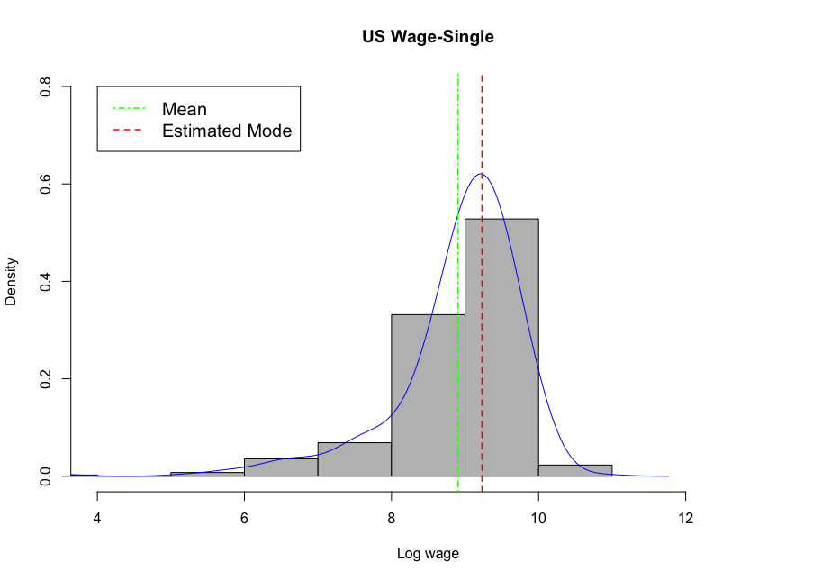
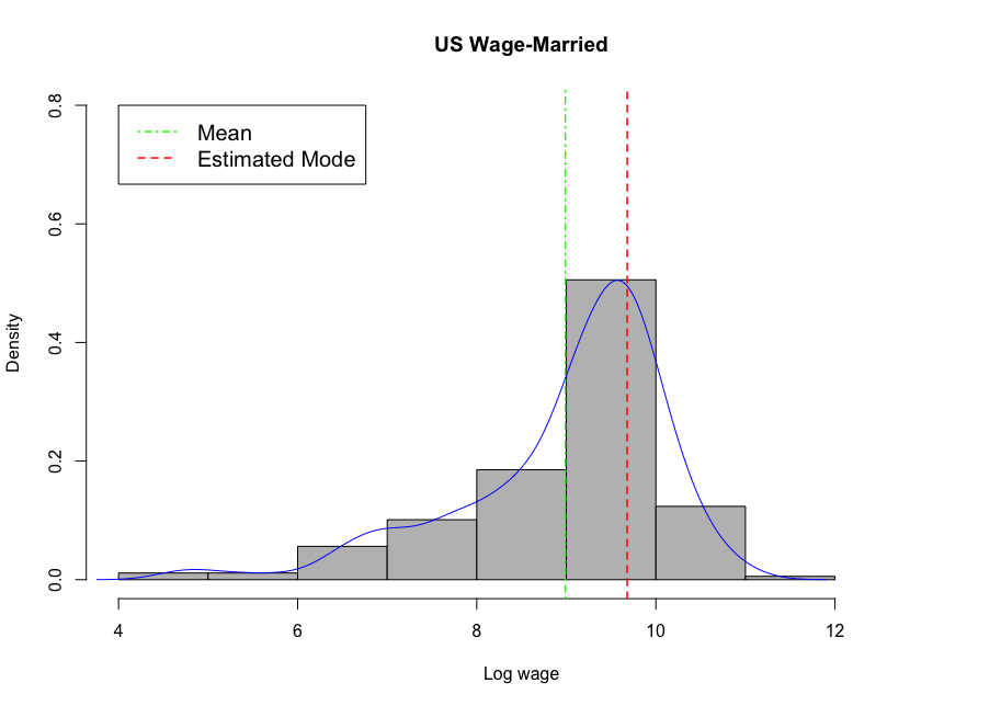
From Figure 1, we have several observations. First, both conditional distributions are skewed, and as argued in Kemp and Santos-Silva, (2012), the mode would be a more intuitive measure of central tendency for such skewed data. Second, our modal estimator provides accurate estimations of conditional modes for both groups. We also present the confidence intervals for the difference of the modes of these two groups (the mode wage of single people minus the mode wage of married people) in Table 5. Since is not contained in both 95% and 99% confidence intervals, we conclude that the difference of the conditional modes between the two groups is statistically significant under those two nominal levels. Therefore, the marital status can possibly be a significant factor contributing to the mode of people’s wage which can be of social interest worth further research.
5 Extension to the increasing dimension case
In this section, we extend the theoretical analysis to the case where the dimension of the covariate vector is allowed to increase with the sample size , i.e., . Such situations arise when we approximate conditional quantile function by a linear combination of basis functions and the approximation error is negligible (in fact, the theory of this section holds as long as the approximation error is at most of the order as the remainder term in the Bahadur representation; see Lemma 16 in Appendix). In this case, is generated as basis functions of a fixed dimensional genuine covariate , i.e., , where vector includes transformations of that have good approximation properties such as Fourier series, splines, and wavelets; cf. Belloni et al., (2015, 2019). It is then of interest to draw simultaneous confidence intervals for the conditional mode along with values of which has fixed dimension although the dimension of increases with .
We first modify Assumption 1 to accommodate the case where . In what follows, constants refer to nonrandom numbers independent of .
Assumption 3.
(i) There exists a constant such that for all ; (ii) There exists such that for all ; (iii) There exists a positive constant such that . The Gram matrix is positive definite with smallest eigenvalue and largest eigenvalue for some constants and ; (iv) Conditions (iv)–(vii) in Assumption 1 hold; (v) For any , there exists a positive constant (that may depend on ) such that ; (vi) for some .
Condition (i) requires the design points of interest to be of the same order . We assume condition (i) to state the results in a concise way, but the order can be relaxed as long as and are of the same order. The modified condition (ii) is assumed to avoid boundary problems of when the dimension increases. We also assume that is bounded by to avoid some technicalities. In particular, under series approximation framework, this assumption is satisfied when is generated from basis functions such as Fourier series, B-splines and wavelet series; cf. Belloni et al., (2015). The condition on the Gram matrix is satisfied under mild conditions on the distribution of the genuine covariate and basis functions; cf. Belloni et al., (2019). Condition (v) is a global identification condition on that is needed to verify the uniform consistency of . If is fixed, then Condition (v) follows automatically as is continuous under Assumption 1 (see the proof of Lemma 8), but if , then and depend on , so that we require Condition (v). Condition (vi) is used to guarantee the Bahadur representation of ; cf. Theorem 2 in Belloni et al., (2019).
Redefine as with
Further, redefine the matrices , , and as in Section 3.3.1 corresponding to the new definition of . For simplicity, we focus here on the studentized case where for . The reason to work with instead of is to better control the residual term in the proof of high dimensional Gaussian approximation result. Normalization by ensures that the norm of is bounded on . The Gaussian approximation with reads as follows.
Theorem 4 (Gaussian approximation when ).
Suppose that ; then Condition (13) reduces to
If we take , then the condition on reduces to . As before, this condition can be relaxed by assuming additional smoothness conditions on the conditional density and using higher order kernels. Similar conditions on appear in the analysis of resampling methods for quantile regression under increasing dimensions; see, e.g., Theorem 5 in Belloni et al., (2019), where .
We now establish the validity of the pivotal bootstrap. The theory for the nonparametric bootstrap can be shown similarly but we omit the details due to the space limit. Redefine with
Let be as in (9) corresponding to the new definition of , and let .
Theorem 5 (Validity of pivotal bootstrap when ).
Remark 7.
The pivotal bootstrap above is the same as the one under the fixed dimension case as the extra normalization by is canceled by the multiplication by (we introduced normalization by to facilitate the proof).
6 Summary
In this paper, we study a novel pivotal bootstrap and the nonparametric bootstrap for simultaneous inference on conditional modes based on a kernel-smoothed Koenker-Bassett quantile estimator. Our bootstrap inference framework allows for simultaneous inference on multiple linear functions of different conditional modes. We establish the validity of the bootstrap inference in both fixed dimension and increasing dimension settings. The numerical results provide strong support of our theoretical results. Several interesting extensions remain, including the extension to time series or longitudinal data. In such settings, we need to modify the bootstraps and develop new technical tools to deal with dependent data. These are beyond the scope of the current paper and left for future research.
Supplemental materials
The supplemental materials contain the wage dataset, R codes and an appendix containing all the proofs, additional simulation results, discussion of model misspecification and quantile crossing, and additional details of the numerical implementation.
The Appendix is organized as follows. We present the proofs of the theoretical results in the main text in Appendices A–D. We provide additional simulation results in Appendix E. We discuss the model misspecification and quantile crossing issues in Appendix F. We provide more implementation details in Appendix G. We present more details of the wage dataset in Appendix H.
Appendix A Auxiliary results for Section 3.3
Proposition 3 (Limit distribution of maximal deviation).
Proposition 3 suggests that we can use the Gumbel approximation to construct simultaneous confidence intervals. The proof shows that if , then is diagonal so that can be approximated by the maximum in absolute value of independent random variables, which can be further approximated (after normalization) by the Gumbel distribution by extreme value theory. Compared with the pivotal bootstrap discussed in Section 3.3.2, the Gumbel approximation leads to analytical critical values, so from a computational perspective, using the Gumbel limit seems more attractive. However, the justification of the Gumbel approximation relies on a nontrivial spacing assumption on ’s (which the pivotal bootstrap does not). More importantly, convergence of normal suprema is known to be extremely slow (Hall,, 1991), so simultaneous confidence intervals constructed from the Gumbel approximation may not have desirable coverage accuracy.
The following lemma is useful to establish the coverage guarantee of our confidence intervals (see Example 3 for more discussion).
Lemma 1.
Let be sequences of random variables defined on a probability space such that (i) is measurable relative to a sub--field (that may depend on ); (ii) and ; (iii) the distribution function of is continuous for each ( need not have a limit distribution). Let denote the conditional -quantile of given . Then .
The proofs of the above two auxiliary results can be found in Appendix C.3.4.
Appendix B Technical tools
In this section, we collect technical tools that will be used in the subsequent proofs. For a probability measure on a measurable space and a class of measurable functions on such that , let denote the -covering number for with respect to the -seminorm . The class is said to be pointwise measurable if there exists a countable subclass such that for every there exists a sequence with pointwise. A function is said to be an envelope for if for all . See Section 2.1 in van der Vaart and Wellner, (1996) for details. For a vector-valued function defined over a set , we define . The norm for a random variable is defined as .
Lemma 2 (Local maximal inequality).
Let be i.i.d. random variables taking values in a measurable space , and let be a pointwise measurable class of (measurable) real-valued functions on with measurable envelope . Suppose that is VC type, i.e., there exist constants and such that
where is taken over all finitely discrete distributions on . Furthermore, suppose that , and let be any positive constant such that . Define . Then
where is a universal constant.
Proof.
See Corollary 5.1 in Chernozhukov et al., (2014). ∎
The following anti-concentration inequality for Gaussian measures (called Nazarov’s inequality in Chernozhukov et al., 2017a ), together with the Gaussian comparison inequality, will play crucial roles in proving the validity of the pivotal bootstrap.
Lemma 3 (Nazarov’s inequality).
Let be a centered Gaussian vector in such that for all and some constant . Then for every and ,
Proof.
See Lemma A.1 in Chernozhukov et al., 2017a ; see also Chernozhukov et al., 2017b . ∎
Lemma 4 (Gaussian comparison).
Let and be centered Gaussian random vectors in with covariance matrices and , respectively, and let . Suppose that for some constant . Then
where is a constant that depends only on .
Proof.
Implicit in the proof Theorem 4.1 in Chernozhukov et al., 2017a . ∎
Appendix C Proofs for Section 3
C.1 Uniform Convergence Rates
We first establish uniform convergence rates of . The following Bahadur representation of the linear quantile regression estimator will be used in the subsequent proofs.
Lemma 5 (Bahadur representation of ).
Under Assumption 1, we have
uniformly in , where i.i.d. that are independent of . In addition, we have
Proof.
Remark 8.
Inspection of the proof shows that where is the conditional distribution function of given .
We first prove the following technical lemma.
Lemma 6.
If Assumption 1 holds, then for , we have
Proof.
Since is supported in , for sufficiently large ,
Consider the function class (which depends on since does). It suffices to show that
To this end, we will apply Lemma 2. The function class is a subset of the pointwise product of the following two function classes (that are independent of ): and . The former function class has envelope and the latter function class has envelope where are some constants independent of . The function class is a subset of a vector space of dimension , so that it is a VC subgraph class with VC index at most (cf. Lemma 2.6.15 in van der Vaart and Wellner, (1996)). Next, since is of bounded variation (i.e., it can be written as the difference of two bounded nondecreasing functions) and the function class is a VC subgraph class (as it is a vector space of dimension ), the function class is VC type in view of Lemma 2.6.18 in van der Vaart and Wellner, (1996). Conclude that, for , there exist positive constants independent of such that
where is taken over all finitely discrete distributions on .
It is not difficult to verify that, by independence between and ,
In addition, (as ). Conclude from Lemma 2 that
This completes the proof. ∎
The following lemma derives uniform convergence rates of .
Lemma 7 (Uniform convergence rates ).
Under Assumption 1, we have
Proof.
Next, consider . We note that
We have for and for by Taylor expansion (recall that is four-times continuously differentiable). Observe that, by Lemma 5 and change of variables,
Replacing by in the first term on the right hand side results in an error of order ; this can be verified by a similar argument to the proof of the preceding lemma. Thus, it remains to bound
where we have used the fact that integrates to . Here, by integration by parts,
Thus, from Lemma 6, we have . This completes the proof. ∎
Remark 9 (Bias of at ).
The bias of can be improved to at by and symmetry of .
Remark 10 (Expansion of ).
Inspection of the proof shows that
| (A3.14) |
uniformly in . Recall that .
C.2 Proofs for Section 3.2
We first prove the uniform consistency of .
Lemma 8 (Uniform consistency of ).
Under Assumption 1, we have .
Proof.
We divide the proof into two steps.
Step 1. We will verify that for any ,
This follows from the following two claims: (i) is jointly continuous in , (ii) is compact in and the observation that is the unique minimizer of , i.e., . Since is continuous in for any fixed under Assumption 1 and also linear (thus convex) in by the linear quantile assumption, Theorem 10.7 in Rockafellar, (1970) implies that is jointly continuous in ). Now, by Berge’s maximum theorem (cf. Theorem 17.31 in Aliprantis and Border, (2006): see also their Lemma 17.6), we see that is continuous in . The preceding discussion also implies that is jointly continuous in . Combining the continuity of and the definition of , we can verify is closed and bounded and therefore compact. Thus, we have verified claims (i) and (ii) and the conclusion of this step follows.
Step 2. We will prove the uniform consistency of . Consider the event . Observe that
The first and third terms on the right hand side are by Lemma 7, while the second term is nonpositive by the definition of . This implies that . The uniform consistency of follows from the fact that the event is included in . ∎
The uniform consistency guarantees that the first order condition for holds for all with probability approaching one, i.e.,
| (A3.15) |
Recall that . Now, we derive an asymptotic linear representation for .
Lemma 9 (Asymptotic linear representation of ).
Under Assumption 1, the following expansion holds uniformly in :
In addition, the first term on the right hand side is uniformly in .
Proof.
From the first order condition (A3.15) coupled with the Taylor expansion, we have
where lies between and . This yields that
The rest of the proof is divided into two steps.
Step 1. We will show that . Observe that uniformly in by Lemma 6, uniformly in by the uniform consistency of , and the map is bounded away from zero on . Thus, we have
However, since , the right hand side on the above equation is by Lemma 6.
Step 2. We wish to derive the conclusion of the lemma. From the preceding discussion, we see that uniformly in , so that
uniformly in . The conclusion of the lemma follows from combining the expansion (A3.14). ∎
We are now in position to prove Proposition 1.
Proof of Proposition 1.
We note that, uniformly in ,
This completes the proof. ∎
C.3 Proofs for Section 3.3
C.3.1 Proof of Theorem 1
We divide the proof into two steps.
Step 1. We will show that
| (A3.16) |
To this end, we verify Conditions (M.1), (M.2), and (E.2) in Proposition 2.1 of Chernozhukov et al., 2017a .
Condition (M.1): For , by definition and Assumption 2,
which is bounded away from zero uniformly over .
Condition (M.2): For ,
Under our assumption, and . In addition,
Likewise, we have .
Condition (E.2): Similarly to the previous case (but bounding by ), we can show that
Thus, we can apply Proposition 2.1 in Chernozhukov et al., 2017a , and the conclusion of this step follows as soon as
but this is satisfied under our assumption.
Step 2. Define and . By Proposition 1, we know that , so that
Thus, for any , we have . Now, for any ,
where the and terms are independent of . Likewise, we have
Since for sufficiently slow under our assumption, we obtain the conclusion of the theorem. ∎
C.3.2 Proofs of Theorem 2 and Proposition 2
We start with proving some technical lemmas. We use to denote the operator norm of a matrix.
Lemma 10.
Under Assumption 1, we have
Proof.
It suffices to show that for any (as the dimension is fixed). Observe that
It is routine to show that the first and second terms on the right hand side are and , respectively; cf. the proof of Lemma 7. By Taylor expansion, the last term can be bounded by . Observe that
This completes the proof. ∎
Lemma 11.
Under Assumption 1, we have
Proof.
For simplicity of notation, let and . The difference can be decomposed as
Observe that
where we have used Lemma 7 in the last line.
Finally, observe that
uniformly in . Likewise, we have
uniformly in . Combining these estimates, we obtain the conclusion of the lemma. ∎
Proof.
This follows from the observation that
∎
We are now in position to prove Theorem 2.
Proof of Theorem 2.
Let be an -dimensional random vector such that conditionally on , . We begin with noting that
We first analyze and . In view of the Gaussian comparison inequality (cf. Lemma 4), to show that , it suffices to verify that
| (A3.17) |
Indeed, by Lemma 12 and the assumption (i) of the theorem, we deduce that the bracket on the left is . Thus, (A3.17) holds under our assumption.
To show that , we apply Proposition 2.1 in Chernozhukov et al., 2017a conditionally on (recall that conditionally on , the vectors are independent with mean zero). By construction, is bounded way from uniformly in with probability approaching one. Similarly to the proof of Theorem 1, we can verify that for . Finally,
Hence, applying Proposition 2.1 in Chernozhukov et al., 2017a , we see that as soon as
but this is satisfied under our assumption. This completes the proof. ∎
Proof of Proposition 2.
Theorem 1 implies that
Since the variances of the coordinates of are bounded, we see that by Lemma 2.2.2 in van der Vaart and Wellner, (1996). Hence, we have
Combining Condition (i) in the statement of Theorem 2, we see that
The rest of the proof is analogous to the last part of Theorem 1. We omit the details for brevity. ∎
C.3.3 Proof of Theorem 3
We start with proving the following uniform Bahadur representation for the quantile regression estimator based on the nonparametric bootstrap samples . We define where is the conditional distribution function of given (see Remark 8).
Lemma 13.
Proof.
We will prove the following equivalent form of (A3.18),
| (A3.19) |
where is a multinomial random vector with parameters and (probabilities) . We will divide the proof into two steps. In the following proof, is a generic constant independent of whose value may vary from line to line.
Step 1. In this step, we will show that . To this end, we introduce the following quantities
where we define and is a sequence of constants to be specified.
In view of the proof of Lemma 3 in Belloni et al., (2019), it suffices to show that , and when . We shall bound the three terms in what follows.
The term is the supremum of a multiplier empirical process, and we will apply a multiplier inequality developed in Han and Wellner, (2019). Define the function class
where . Then . We first verify that
| (A3.20) |
This can be proved as follows
For any , by Theorem 2.14.1 in van der Vaart and Wellner, (1996),
This leads to (A3.20).
Now, by Lemma 2.3.6 in van der Vaart and Wellner, (1996), (A3.20) implies the following bound for the symmetrized empirical process
where () are i.i.d. Rademacher random variables independent of the data. Given the above bound, we can apply Corollary 1 in Han and Wellner, (2019) (recall is fixed) to conclude that
This implies that .
We can bound similarly to . Define the function class
so that . Applying Lemma 2, we have
Now we apply Corollary 1 in Han and Wellner, (2019) (with for some arbitrary small in the proof there) to conclude that
which implies that .
For , we proceed as in Lemma 33 of Belloni et al., (2019) to see that
where lies on the line segment between and . We further bound the right-hand side as
These bounds imply the conclusion of this step, in view of the proof of Lemma 3 in Belloni et al., (2019).
Step 2. We finish the proof of the lemma. Define
It suffices to show that for arbitrarily small . We note that, by Step 1, for any arbitrarily slowly, with holds with probability approaching one. Hence, taking such , with probability ,
where . By Step 1, taking sufficiently slowly, we have
To bound , from the proof of Lemma 34 in Belloni et al., (2019),we can deduce that
We further bound the right-hand side as
Hence we have shown that
which finishes the proof. ∎
Define and .
Lemma 14.
Under Assumption 1, we have
Proof.
Recall that . The difference can be decomposed as
We define
We first bound . Define the function class
Then we have . Applying Lemma 2, we have
Hence we have shown that
For , we define the following function class
Then we have
Similarly to the previous case, by using Lemma 2, we can show that
which implies that . Combining the above bounds, we obtain the desired result. ∎
We are now in position to prove Theorem 3.
Proof of Theorem 3.
We begin with noting that, using the Bahadur representation in Lemma 13,we can establish the following asymptotic linear representation for the bootstrap mode estimator by a similar analysis to the proof of Theorem 1 coupled with the multiplier inequality techniques as in the proof of Lemma 13:
| (A3.21) | ||||
where . Hence we have
Now, we divide the rest of the proof into two steps.
Step 1. We will show that
| (A3.22) |
We note that
where and recall .
We first analyze and . In view of the Gaussian comparison inequality (cf. Lemma 4), to show that , it suffices to verify that
| (A3.23) |
Indeed, by Lemma 15 and Condition (i) of the theorem, we can deduce that the bracket on the left hand side is . Thus, (A3.23) holds under our assumption.
To show that , we apply Proposition 2.1 in Chernozhukov et al., 2017a conditionally on (recall that conditionally on , the vectors are independent with mean zero). By construction, is bounded away from zero uniformly over with probability approaching one. Similarly to the proof of Theorem 1, we can verify that for . Finally,
Hence, applying Proposition 2.1 in Chernozhukov et al., 2017a , we see that as soon as
but this is satisfied under our assumption. This completes Step 1.
Step 2. We finish the proof by a similar analysis as Step 2 in the proof of Theorem 1. Define . Combining the analysis before Step 1 and the fact that , we have . Similarly to Step 2 in the proof of Theorem 1, we can show that The rest of the proof is analogous to the last part of Theorem 1. We omit the details for brevity. ∎
C.3.4 Proofs for Appendix A
Proof of Proposition 3.
Proof of Lemma 1.
Let denote the -quantile of . By assumption, we may choose a sequence such that
The latter follows from the fact that the Ky Fan metric metrizes convergence in probability. Define the event . On this event,
so that . Thus,
Likewise, on the event ,
so that . Arguing as in the previous case, we see that . This completes the proof.
∎
Appendix D Proofs for Section 5
Recall that is the unit sphere in , i.e., . Also recall that in Section 5, we allow .
D.1 Proof of Theorem 4
Overall, the proof is analogous to that of Theorem 1. The following Banadur representation is taken from Belloni et al., (2019).
Lemma 16.
Proof.
See Theorems 1 and 2 in Belloni et al., (2019). ∎
The rates of convergence of change as follows.
Lemma 17.
Under the conditions of Theorem 4, we have
Proof.
We divide the proof into two steps.
Step 1. We will show that
for . The proof is analogous to that of Lemma 6, so we only point out required modifications. The envelope function should be modified to for some constant , and note that the VC constant is of order . Observe that
and (as ). Applying Lemma 2 leads to the above rates.
Step 2. We will show the conclusion of the lemma. This part is analogous to the proof of Lemma 7, so we only point out required modifications. The follows from Lemma 16 and Taylor expansion. For , combining Lemma 16, change of variables, and Taylor expansion, we can bound by
Replacing by in the first term on the right hand side results in an error of order . Given Step 1, the rest of the proof is completely analogous to the last part of the proof of Lemma 7. ∎
Remark 11 (Expansion of ).
Inspection of the proof shows that
uniformly in , and the uniform rate over of the first term on the right hand side is .
Recall the definition of . In view of the proof of Lemma 8, the following lemma follows relatively directly from Lemma 17.
Lemma 18.
Under the conditions of Theorem 4, the following asymptotic linear representation holds uniformly in :
where i.i.d. independent of . In addition, we have
We are now in position to prove Theorem 4.
Proof of Theorem 4.
As before, we split the proof into two parts.
Step 1. We will apply Proposition 2.1 in Chernozhukov et al., 2017a to . To this end, we will check Conditions (M.1), (M.2), and (E.1) of Chernozhukov et al., 2017a . Condition (M.1) follows automatically, so we will verify Conditions (M.2) and (E.1).
Condition (M.2). Recall that for all . Observe that
where we used the fact that
This implies that . Likewise, .
Condition (E.2). Since , we have .
Thus, applying Proposition 2.1 in Chernozhukov et al., 2017a , we have
provided that
which is satisfied under our assumption.
D.2 Proof of Theorem 5
Define with
Further, define , with , and .
The following operator norm bound is in parallel to Lemma 10 for the fixed dimensional case.
Lemma 19.
Under the conditions of Theorem 5, we have
Proof.
Observe that the left hand side can be bounded by
where . By Taylor expansion and , we see that . Next, applying the local maximal inequality (Lemma 2) combined with the fact that , we can show that . Finally, the term is bounded by
where we used the observation that is bounded in . Conclude that . ∎
Similarly, we have the following lemma in parallel to Lemma 11.
Lemma 20.
Under Assumption 3, we have
Proof.
The proof is analogous to the proof of Lemma 11, given that and we added normalization by in the definition of . The only missing part is a bound on
but Rudelson’s inequality yields that the above term is ; cf. Rudelson, (1999).
∎
We are now in position to prove Theorem 5.
Proof of Theorem 5.
Observe that
| (A4.25) |
where . The first term on the right hand side of (A4.25) is bounded by
where conditionally on . For , we can apply Proposition 2.1 in Chernozhukov et al., 2017a conditionally on . Similarly to the last part of the proof of Theorem 2, we can show that if
which is satisfied under our assumption. We can analyze and as in the proof of Theorem 2 and show that if and , which is satisfied under our assumption.
Appendix E Additional simulation results
E.1 Nonparametric bootstrap pointwise confidence intervals
In this section, we present simulation results for the nonparametric bootstrap. Due to the heavy computational burden of the nonparametric bootstrap, we only consider pointwise confidence intervals in the simulation. We consider the , and models as in Section 4.1.2, together with the same subsample sizes, , and , and repetition number . The results are presented in Tables A1–A3.
| Design point | Sample size | Coverage probability | Median length | Interquartile range | |||
|---|---|---|---|---|---|---|---|
| 95% | 99% | 95% | 99% | 95% | 99% | ||
| =0.3 | 92.4% | 97.6% | 0.80 | 1.14 | 0.38 | 0.52 | |
| 93.2% | 98.8% | 0.69 | 0.95 | 0.29 | 0.39 | ||
| 92% | 99.2% | 0.57 | 0.79 | 0.25 | 0.33 | ||
| =0.5 | 92.4% | 98.4% | 0.91 | 1.25 | 0.40 | 0.57 | |
| 93.4% | 98.2% | 0.76 | 1.05 | 0.30 | 0.44 | ||
| 93.4% | 98% | 0.64 | 0.88 | 0.22 | 0.32 | ||
| =0.7 | 92.4% | 98.6% | 1.10 | 1.57 | 0.54 | 0.80 | |
| 91.4% | 97.6% | 0.91 | 1.26 | 0.40 | 0.58 | ||
| 93.8% | 97.6% | 0.79 | 1.07 | 0.27 | 0.40 | ||
| Design point | Sample size | Coverage probability | Median length | Interquartile range | |||
|---|---|---|---|---|---|---|---|
| 95% | 99% | 95% | 99% | 95% | 99% | ||
| =0.3 | 87.8% | 95.8% | 2.85 | 4.31 | 2.70 | 4.06 | |
| 86.2% | 94.4% | 1.86 | 3.27 | 2.05 | 3.61 | ||
| 89.2% | 95.4% | 1.47 | 2.69 | 2.07 | 3.36 | ||
| =0.5 | 85% | 95.2% | 3.28 | 5.05 | 2.86 | 4.14 | |
| 88% | 95.8% | 2.03 | 3.57 | 2.39 | 3.99 | ||
| 84.4% | 92.6% | 1.55 | 2.76 | 1.99 | 3.49 | ||
| =0.7 | 82% | 92.8% | 4.51 | 6.64 | 4.27 | 6.69 | |
| 86.2% | 96% | 2.76 | 5.39 | 3.10 | 4.43 | ||
| 83.6% | 94.4% | 1.75 | 3.13 | 2.07 | 3.95 | ||
| Design point | Sample size | Coverage probability | Median length | Interquartile range | |||
|---|---|---|---|---|---|---|---|
| 95% | 99% | 95% | 99% | 95% | 99% | ||
| =0.7 | 94.8% | 99% | 1.05 | 1.62 | 1.55 | 2.62 | |
| 92.2% | 98.4% | 0.78 | 1.27 | 1.01 | 1.91 | ||
| 94.8% | 98.8% | 0.67 | 1.08 | 0.92 | 1.32 | ||
| =0.9 | 94% | 99.4% | 1.11 | 1.59 | 1.25 | 1.77 | |
| 94.0% | 98% | 0.84 | 1.42 | 1.18 | 1.57 | ||
| 94.8% | 98% | 0.60 | 1.04 | 0.86 | 1.25 | ||
| =1.1 | 94% | 99% | 0.80 | 1.49 | 1.05 | 1.17 | |
| 95.2% | 99.2% | 0.56 | 1.08 | 0.80 | 1.14 | ||
| 92.8% | 97.8% | 0.36 | 0.60 | 0.39 | 0.74 | ||
From the simulation results, the nonparametric bootstrap confidence intervals achieve close to nominal coverage probabilities under large sample sizes for the lmNormal and Nonlinear models. For the lmLognormal model, the nonparametric bootstrap confidence intervals have lower coverage probabilities than the nominal level. This may be due to the slow convergence rate of the bootstrap approximation to the sampling distribution under such a data generating process. Compared with the pivotal bootstrap confidence intervals in the other two models, the nonparametric bootstrap provides shorter and more stable confidence intervals, i.e., less variable interval lengths, in the lmNormal model while the pivotal bootstrap performs better in the Nonlinear model.
To further demonstrate the computational advantage of the pivotal bootstrap over the nonparametric bootstrap, we report the average running time of these two bootstraps in the Nonlinear model with design point (results in other scenarios are similar). The simulation results are obtained in the R environment with 28 Intel Xeon processors and 240 Gbytes RAM over Red Hat OpenStack Platform. We measure the average running time in seconds and report the results in Table A4. From the table, we can see that the pivotal bootstrap requires substantially less computational time than the nonparametric bootstrap as predicted in Remark 6 in the main text.
| Design point | Sample size | Pivotal bootstrap | Nonparametric bootstrap |
|---|---|---|---|
| =0.9 | 1.02 | 22.23 | |
| 1.43 | 33.79 | ||
| 2.27 | 58.08 |
E.2 Mean squared error comparison with existing modal estimators
In the following, we present the mean squared error of our modal estimator , which is defined by
where is the true conditional mode and is our modal estimator in the -th repetition. We compare our method with existing methods by Ota et al., (2019), Kemp and Santos-Silva, (2012) and Yao and Li, (2014). We consider the , and models as in Section 4.1.2. The same subsample sizes, , and , and repetition number are considered. The results are presented in Tables A5–A7. The KS-YL estimator refers to the linear modal estimator studied by Kemp and Santos-Silva, (2012) and Yao and Li, (2014).
| Design point | Sample size | Our estimator | Ota et al., (2019) | KS-YL estimator |
|---|---|---|---|---|
| =0.3 | 0.020 | 0.063 | 0.207 | |
| 0.018 | 0.043 | 0.208 | ||
| 0.010 | 0.032 | 0.275 | ||
| =0.5 | 0.026 | 0.091 | 0.712 | |
| 0.017 | 0.063 | 0.713 | ||
| 0.012 | 0.047 | 0.928 | ||
| =0.7 | 0.109 | 0.167 | 1.559 | |
| 0.026 | 0.128 | 1.840 | ||
| 0.024 | 0.103 | 1.954 |
| Design point | Sample size | Our estimator | Ota et al., (2019) | KS-YL estimator |
|---|---|---|---|---|
| =0.3 | 0.286 | 0.329 | 0.146 | |
| 0.162 | 0.296 | 0.124 | ||
| 0.118 | 0.259 | 0.066 | ||
| =0.5 | 0.421 | 0.508 | 0.204 | |
| 0.219 | 0.466 | 0.160 | ||
| 0.151 | 0.410 | 0.094 | ||
| =0.7 | 0.845 | 0.774 | 0.407 | |
| 0.491 | 0.657 | 0.269 | ||
| 0.217 | 0.605 | 0.224 |
| Design point | Sample size | Our estimator | Ota et al., (2019) | KS-YL estimator |
|---|---|---|---|---|
| =0.3 | 0.0090 | 0.0023 | 0.051 | |
| 0.0071 | 0.00082 | 0.041 | ||
| 0.0044 | 0.00045 | 0.031 | ||
| =0.5 | 0.016 | 0.0052 | 0.075 | |
| 0.010 | 0.0046 | 0.063 | ||
| 0.0086 | 0.0043 | 0.049 | ||
| =0.7 | 0.026 | 0.025 | 0.074 | |
| 0.017 | 0.023 | 0.068 | ||
| 0.012 | 0.022 | 0.052 |
From the simulation results, while no method dominates in all the three scenarios, the proposed modal estimator performs reasonably well uniformly in all the settings. In particular, our estimator and Ota et al., (2019)’s estimator outperform the KS-YL linear modal estimator in the Nonlinear model as expected.
E.3 Simulation results for the pivotal bootstrap testing
In this section, we consider testing significance of a covariate on the conditional mode. Suppose covariate where is continuous and is binary (0 or 1). We want to test the null hypothesis versus the alternative hypothesis , where is the conditional mode of given and . We will generate according to and . For the outcome , two generation schemes are considered: (1) and (2) , where we take and in both models. The corresponding mode functions are and , respectively. Therefore, the two generation schemes correspond to being true and false respectively which allows us to evaluate both power and size of our bootstrap testing procedure. We will take or in the simulation. In the current setup, the limiting Gaussian distribution given by Theorem 1 is one dimensional and the corresponding variance can be calculated explicitly based on the above setup. Therefore, an oracle test procedure can be constructed by using the quantiles of the corresponding limiting Gaussian distribution to define the test rejection region. We will compare the performance of our bootstrap testing with this benchmark oracle testing.
We conduct hypothesis testing of nominal level and for taking value at 0.3, 0.5 and 0.7. For each value of , three different sample sizes from 500 to 2000 are considered. We report the empirical size and power of both bootstrap testing and oracle testing based on 500 simulations in Tables A8 and A9.
| Bootstrap testing | Oracle testing | ||||||||
|---|---|---|---|---|---|---|---|---|---|
| Design Point | Sample size | Size | Power | Size | Power | ||||
| 0.05 | 0.01 | 0.05 | 0.01 | 0.05 | 0.01 | 0.05 | 0.01 | ||
| 0 | 0 | 0.622 | 0.348 | 0.012 | 0 | 1 | 0.996 | ||
| 0.006 | 0.002 | 0.814 | 0.628 | 0.022 | 0.004 | 1 | 1 | ||
| 0 | 0 | 0.932 | 0.874 | 0.032 | 0.002 | 1 | 1 | ||
| 0.004 | 0 | 0.55 | 0.322 | 0.016 | 0.002 | 0.994 | 0.984 | ||
| 0.004 | 0 | 0.794 | 0.608 | 0.048 | 0.002 | 1 | 0.996 | ||
| 0.004 | 0 | 0.928 | 0.84 | 0.022 | 0.006 | 1 | 1 | ||
| 0.002 | 0 | 0.596 | 0.408 | 0.012 | 0.02 | 0.998 | 0.994 | ||
| 0 | 0 | 0.816 | 0.644 | 0.024 | 0.006 | 0.998 | 0.996 | ||
| 0.004 | 0 | 0.928 | 0.842 | 0.038 | 0.006 | 1 | 1 | ||
| Design point | Sample size | Bootstrap testing | Oracle testing | ||
|---|---|---|---|---|---|
| 0.05 | 0.01 | 0.05 | 0.01 | ||
| 0.39 | 0.176 | 0.978 | 0.894 | ||
| 0.66 | 0.406 | 0.992 | 0.98 | ||
| 0.858 | 0.696 | 1 | 1 | ||
| 0.392 | 0.18 | 0.962 | 0.846 | ||
| 0.628 | 0.396 | 0.992 | 0.968 | ||
| 0.874 | 0.706 | 1 | 0.998 | ||
| 0.416 | 0.21 | 0.976 | 0.894 | ||
| 0.66 | 0.432 | 0.996 | 0.982 | ||
| 0.872 | 0.708 | 1 | 0.998 | ||
From the tables, the Type \@slowromancapi@ errors are well preserved for both tests at three design points while the bootstrap testing committed slightly fewer Type \@slowromancapi@ errors. We can see the decrease of power of both bootstrap testing and oracle testing under the same design point () and subsample size () as gets smaller. For a fixed design point, the power of both tests approaches with the increasing subsample size which supports our theory. In particular, the good performance of the oracle testing justifies our normal approximation theory. The performance of the proposed bootstrap testing is inferior to the oracle testing under the same design point and subsample size. This may due to several reasons including the bootstrap approximation error and the bias in the estimation of the nuisance parameters. However, the performance of bootstrap testing is reasonable when the sample size is sufficiently large which agrees with our asymptotic theory.
We also remark that we here test the significance of the covariates for the conditional mode by testing the change of the conditional mode due to the change of design points, instead of testing the corresponding coefficient in the quantile regression slope vector. This is due to the following observation. Although we assume a linear quantile model, it does not imply a direct modeling on the conditional mode function. That is, the conditional mode depends on the covariates in an implicit way under our quantile-based mode regression, i.e. under our modeling, the mode function is where the coordinates of are functions of that may have arbitrary forms (as long as they satisfy some natural restrictions resulted from quantile functions). It is possible that one coefficient of the is nonzero while the corresponding covariate does not contribute to the conditional mode function. This is in contrast to the linear modal regression where the mode function is assumed to be where is a constant vector (independent of ) and therefore testing the significance of the covariates is equivalent to testing the coefficients in being or not.
E.4 Pivotal bootstrap confidence intervals using oracle information
In this section, we provide simulation results of pivotal bootstrap inference using oracle model information, i.e., we estimate the nuisance parameters in the influence function based on the underlying true density or conditional quantile function. We reexamine the setups in Section 4.1.2 and the corresponding results for pointwise confidence intervals are presented in Tables A10 to A12 and Table A13 for approximate confidence bands.
| Design point | Sample size | Coverage probability | Median length | Interquartile range | |||
|---|---|---|---|---|---|---|---|
| 95% | 99% | 95% | 99% | 95% | 99% | ||
| =0.3 | 95.4% | 99.6% | 0.94 | 1.24 | 0.16 | 0.19 | |
| 95% | 99.2% | 0.79 | 1.02 | 0.13 | 0.14 | ||
| 96.6% | 99% | 0.64 | 0.85 | 0.08 | 0.10 | ||
| =0.5 | 95.2% | 99.2% | 1.04 | 1.38 | 0.24 | 0.32 | |
| 94.6% | 98.6% | 0.86 | 1.14 | 0.15 | 0.20 | ||
| 95% | 99.2% | 0.71 | 0.94 | 0.11 | 0.13 | ||
| =0.7 | 96.6% | 98.8% | 1.29 | 1.70 | 0.37 | 0.41 | |
| 96% | 99.4% | 1.06 | 1.42 | 0.22 | 0.27 | ||
| 95.6% | 99.6% | 0.88 | 1.16 | 0.16 | 0.21 | ||
| Design point | Sample size | Coverage probability | Median length | Interquartile range | |||
|---|---|---|---|---|---|---|---|
| 95% | 99% | 95% | 99% | 95% | 99% | ||
| =0.3 | 77% | 80.6% | 1.44 | 1.86 | 0.91 | 1.20 | |
| 94% | 96% | 1.34 | 1.75 | 0.52 | 0.63 | ||
| 96.4% | 99.8% | 1.01 | 1.33 | 0.28 | 0.35 | ||
| =0.5 | 83.4% | 84.8% | 2.07 | 2.67 | 1.31 | 1.77 | |
| 96% | 97.8% | 1.85 | 2.43 | 0.79 | 1.00 | ||
| 97.4% | 99.8% | 1.52 | 2.02 | 0.54 | 0.69 | ||
| =0.7 | 76.6% | 81% | 2.33 | 3.19 | 1.65 | 2.26 | |
| 93.4% | 94.8% | 2.25 | 3.03 | 1.36 | 1.61 | ||
| 96.2% | 98.6% | 1.84 | 2.43 | 0.76 | 0.92 | ||
| Design point | Sample size | Coverage probability | Median length | Interquartile range | |||
|---|---|---|---|---|---|---|---|
| 95% | 99% | 95% | 99% | 95% | 99% | ||
| =0.7 | 92.4% | 97.4% | 0.58 | 0.73 | 0.48 | 0.47 | |
| 96% | 98.8% | 0.45 | 0.59 | 0.45 | 0.49 | ||
| 97% | 99% | 0.35 | 0.46 | 0.22 | 0.29 | ||
| =0.9 | 94.4% | 97.2% | 0.62 | 0.81 | 0.46 | 0.57 | |
| 94.8% | 97.6% | 0.50 | 0.66 | 0.24 | 0.32 | ||
| 96% | 98.8% | 0.45 | 0.58 | 0.19 | 0.24 | ||
| =1.1 | 93.2% | 96.8% | 0.53 | 0.70 | 0.18 | 0.26 | |
| 94.8% | 97.6% | 0.46 | 0.59 | 0.17 | 0.21 | ||
| 94% | 98% | 0.37 | 0.48 | 0.10 | 0.14 | ||
| Models | Sample size | Coverage probability | Median length | ||
|---|---|---|---|---|---|
| 95% | 99% | 95% | 99% | ||
| lmNormal | 94.8% | 98.6% | 1.14 | 1.48 | |
| 94.6% | 98.8% | 0.97 | 1.22 | ||
| 93.4% | 98.8% | 0.79 | 1.02 | ||
| lmLognormal | 82.6% | 84.2% | 2.39 | 3.06 | |
| 95.2% | 97.1% | 2.03 | 2.65 | ||
| 97.6% | 99.4% | 1.73 | 2.18 | ||
| Nonlinear | 94.6% | 97.6% | 1.12 | 1.23 | |
| 96% | 97.8% | 0.82 | 0.98 | ||
| 94.2% | 98% | 0.49 | 0.59 | ||
From the simulation results, the oracle confidence intervals achieve close to nominal level coverage probabilities when the sample size is sufficiently large, which supports our theoretical results.
Appendix F Additional discussion: model misspecification and quantile crossing
In theory, the quantile crossing problem does not happen since we assume that
See Condition (v) in Assumption 1. This implies the quantile function is strictly increasing in the quantile index . Further, under our assumption, is uniformly consistent over and (see Lemma 7 in Appendix), so that the estimated conditional quantile function is strictly increasing on with probability approaching one.
Of course, the quantile crossing problem may happen in the finite sample even if the model is correctly specified (Koenker 2005). Several methods have been proposed to deal with the quantile crossing problem in the literature, cf. He (1997), Chernozhukov et al. (2009) and Bondell et al. (2010). We can apply any of such monotonization methods to the estimated conditional quantile function to prevent quantile crossing; our theoretical results continue to hold for such a monotonized conditional quantile estimate, as the monotonized estimate agrees with the vanilla conditional quantile estimate with probability approaching one.
Under model misspecification, the fitted linear quantile function can be interpreted as the best linear approximation to the quantile function under some quadratic discrepancy measure cf. section 2.9 in Koenker (2005) and Angrist et al. (2006). Thus, our can be interpreted as a minimization point of the derivative of the best linear approximation. Significant number of quantile crossings also implies the misspecification of the model (Koenker (2005)). If this happens, we suggest using the series approximation approach of our method as discussed in Section 5.
Appendix G More implementation details of Section 4.1
In this section, we provide more implementation details of estimating in the simulation. We use the following kernel estimator for (recall that ):
where is the observed value of in the -th data point. We use the Gaussian kernel for and the Epanechnikov kernel for in the simulation. We use the following bandwidths for covariate and in our simulation, respectively:
| (A7.26) |
where is the corresponding sample standard deviation and . To select in a data-driven approach, we propose the following procedure. The procedure is motivated by the -based bandwidth selector in Bissantz et al., (2007).
-
Step 1.
Choose a proper grid with values for .
-
Step 2.
Generate a dataset of size and then compute by taking () and denote the resulting estimator by . Compute (). Choose for some . Repeat the computation of for times to get and denote the mode of s by .
-
Step 3.
Choose a subgrid centering at . Then we proceed as Step 2 and output the final selected .
In fact, we may iterate the above procedure for more times by using a further subgrid based on the output of Step 3. However, we find the above three-step algorithm works reasonably well in our numerical experiments. In our simulation of pointwise confidence intervals, we take as a equally spaced grid on with ; ( for lmNormal and for lmLogNormal and Nonlinear); and of length . To relieve the computational burden, for each model we only select once for a particular design point at sample size . The selected values of for pointwise confidence intervals are reported in Tables A14 and A15. For the simulation of confidence bands, we use a common for all the different design points in the considered models to reduce the computational burden and the corresponding values are reported in Table A16. Based on our numerical experience, we recommend a slightly larger than the pointwisely selected for the confidence bands if a common is used. In practice, we may use pointwisely selected for different design points when constructing confidence bands. For the practical use, in Step 2 may be taken as the bootstrap subsamples.
| Models | |||
|---|---|---|---|
| lmNormal | 0.75 | 0.85 | 0.95 |
| lmLogormal | 0.35 | 0.45 | 0.55 |
| Models | |||
|---|---|---|---|
| Nonlinear | 0.55 | 0.65 | 0.75 |
| Models | lmNormal | lmLognormal | Nonlinear |
|---|---|---|---|
| 1.00 | 0.60 | 0.80 |
Appendix H More details on the U.S. wage dataset
The data are extracted from U.S. 1980 1% metro sample from the Integrated Public Use Microdata Series (IPUMS) website (Ruggles et al.,, 2020). We first collect data of black and white people aged 30 - 60 with at least kindergarten level of education (nursery school is excluded), with positive annual earnings in the year preceding the census. Individuals with missing values for age, education and earnings are also excluded from the sample. Then we randomly sample people from the single and married groups, respectively and combine the resulting data as the final U.S. wage dataset.
The wage variable (wage) is the log annual wage, calculated as the log of the reported annual income from work in the previous year. The education variable (edu) corresponds to the highest grade of school completed starting from which indicates the kindergarten level. For the marital status variable (marital_status), 0 stands for ”being single” and 1 stands for ”being married”. For the race variable (race), 1 corresponds to white people and 2 corresponds to black people. For the sex variable (sex), 1 corresponds to male and 2 correspond to female.
References
- Aliprantis and Border, (2006) Aliprantis, C. D. and Border, K. C. (2006). Infinite Dimensional Analysis: a Hitchhiker’s Guide. Springer, Berlin; London.
- Autor et al., (2008) Autor, D. H., Katz, L. F., and Kearney, M. S. (2008). Trends in us wage inequality: Revising the revisionists. The Review of Economics and Statistics, 90(2):300–323.
- Bamford et al., (2008) Bamford, S. P., Rojas, A. L., Nichol, R. C., Miller, C. J., Wasserman, L., Genovese, C. R., and Freeman, P. E. (2008). Revealing components of the galaxy population through non-parametric techniques. Monthly Notices of the Royal Astronomical Society, 391(2):607–616.
- Belloni et al., (2019) Belloni, A., Chernozhukov, V., Chetverikov, D., and Fernández-Val, I. (2019). Conditional quantile processes based on series or many regressors. Journal of Econometrics, 213(1):4 – 29.
- Belloni et al., (2015) Belloni, A., Chernozhukov, V., Chetverikov, D., and Kato, K. (2015). Some new asymptotic theory for least squares series: Pointwise and uniform results. Journal of Econometrics, 186:345–366.
- Bissantz et al., (2007) Bissantz, N., Dümbgen, L., Holzmann, H., and Munk, A. (2007). Non-parametric confidence bands in deconvolution density estimation. Journal of the Royal Statistical Society: Series B (Statistical Methodology), 69(3):483–506.
- Bound and Krueger, (1991) Bound, J. and Krueger, A. B. (1991). The extent of measurement error in longitudinal earnings data: Do two wrongs make a right? Journal of Labor Economics, 9(1):1–24.
- Buchinsky, (1994) Buchinsky, M. (1994). Changes in the U.S. wage structure 1963-1987: Application of quantile regression. Econometrica, 62(2):405–458.
- Chacón, (2018) Chacón, J. (2018). The modal age of statistics. arXiv:1807.02789.
- Chen and Kato, (2020) Chen, X. and Kato, K. (2020). Jackknife multiplier bootstrap: finite sample approximations to the u-process supremum with applications. Probability Theory and Related Fields, 176(3):1097–1163.
- Chen, (2018) Chen, Y.-C. (2018). Modal regression using kernel density estimation: A review. Wiley Interdisciplinary Reviews: Computational Statistics, 10(4):e1431.
- Chen et al., (2016) Chen, Y.-C., Genovese, C. R., Tibshirani, R. J., and Wasserman, L. (2016). Nonparametric modal regression. The Annals of Statistics, 44(2):489–514.
- Cheng, (1995) Cheng, Y. (1995). Mean shift, mode seeking, and clustering. IEEE Transactions on Pattern Analysis and Machine Intelligence, 17(8):790–799.
- Chernozhukov et al., (2014) Chernozhukov, V., Chetverikov, D., and Kato, K. (2014). Gaussian approximation of suprema of empirical processes. The Annals of Statistics, 42(4):1564–1597.
- Chernozhukov et al., (2016) Chernozhukov, V., Chetverikov, D., and Kato, K. (2016). Empirical and multiplier bootstraps for suprema of empirical processes of increasing complexity, and related gaussian couplings. Stochastic Processes and their Applications, 126(12):3632–3651.
- (16) Chernozhukov, V., Chetverikov, D., and Kato, K. (2017a). Central limit theorems and bootstrap in high dimensions. The Annals of Probability, 45(4):2309–2352.
- (17) Chernozhukov, V., Chetverikov, D., and Kato, K. (2017b). Detailed proof of nazarov’s inequality. arXiv:1711.10696.
- Chernozhukov et al., (2009) Chernozhukov, V., Hansen, C., and Jansson, M. (2009). Finite sample inference for quantile regression models. Journal of Econometrics, 152:93–103.
- Deng and Zhang, (2017) Deng, H. and Zhang, C.-H. (2017). Beyond gaussian approximation: Bootstrap for maxima of sums of independent random vectors. arXiv preprint arXiv:1705.09528.
- Einbeck and Tutz, (2006) Einbeck, J. and Tutz, G. (2006). Modelling beyond regression functions: an application of multimodal regression to speed–flow data. Journal of the Royal Statistical Society: Series C (Applied Statistics), 55(4):461–475.
- Feng et al., (2020) Feng, Y., Fan, J., and Suykens, J. A. (2020). A statistical learning approach to modal regression. Journal of Machine Learning Research, 21(2):1–35.
- Gutenbrunner and Jurecková, (1992) Gutenbrunner, C. and Jurecková, J. (1992). Regression rank scores and regression quantiles. The Annals of Statistics, pages 305–330.
- Hall, (1991) Hall, P. (1991). On convergence rates of suprema. Probability Theory and Related Fields, 89(4):447–455.
- Han and Wellner, (2019) Han, Q. and Wellner, J. A. (2019). Convergence rates of least squares regression estimators with heavy-tailed errors. Annals of Statistics, 47(4):2286–2319.
- He, (2017) He, X. (2017). Resampling methods. In Handbook of quantile regression, pages 7–19. Chapman and Hall/CRC.
- He and Shao, (1996) He, X. and Shao, Q.-M. (1996). A general bahadur representation of m-estimators and its application to linear regression with nonstochastic designs. The Annals of Statistics, 24(6):2608–2630.
- Heckman et al., (2001) Heckman, D. S., Geiser, D. M., Eidell, B. R., Stauffer, R. L., Kardos, N. L., and Hedges, S. B. (2001). Molecular evidence for the early colonization of land by fungi and plants. Science, 293(5532):1129–1133.
- Hedges and Shah, (2003) Hedges, S. B. and Shah, P. (2003). Comparison of mode estimation methods and application in molecular clock analysis. BMC Bioinformatics, 4(1):31.
- Ho et al., (2017) Ho, C., Damien, P., and Walker, S. (2017). Bayesian mode regression using mixtures of triangular densities. Journal of Econometrics, 197(2):273–283.
- Hu and Schennach, (2008) Hu, Y. and Schennach, S. M. (2008). Instrumental variable treatment of nonclassical measurement error models. Econometrica, 76(1):195–216.
- Kemp and Santos-Silva, (2012) Kemp, G. C. and Santos-Silva, J. (2012). Regression towards the mode. Journal of Econometrics, 170(1):92–101.
- Khardani and Yao, (2017) Khardani, S. and Yao, A. (2017). Non linear parametric mode regression. Communications in Statistics-Theory and Methods, 46(6):3006–3024.
- Koenker, (2005) Koenker, R. (2005). Quantile Regression. Econometric Society Monographs. Cambridge University Press.
- Koenker, (2017) Koenker, R. (2017). Quantile regression: 40 years on. Annual Review of Economics, 9:155–176.
- Koenker and Bassett, (1978) Koenker, R. and Bassett, G. (1978). Regression quantiles. Econometrica, 46(1):33–50.
- Krief, (2017) Krief, J. M. (2017). Semi-linear mode regression. The Econometrics Journal, 20(2):149–167.
- Leadbetter et al., (1983) Leadbetter, M., Lindgren, G., and Rootzén, H. (1983). Extremes and Related Properties of Random Sequences and Processes. Springer.
- Lee, (1989) Lee, M.-J. (1989). Mode regression. Journal of Econometrics, 42(3):337–349.
- Lee, (1993) Lee, M.-J. (1993). Quadratic mode regression. Journal of Econometrics, 57(1-3):1–19.
- Lee and Kim, (1998) Lee, M.-J. and Kim, H. (1998). Semiparametric econometric estimators for a truncated regression model: A review with an extension. Statistica Neerlandica, 52(2):200–225.
- Manski, (1991) Manski, C. F. (1991). Regression. Journal of Economic Literature, 29(1):34–50.
- Ota et al., (2019) Ota, H., Kato, K., and Hara, S. (2019). Quantile regression approach to conditional mode estimation. Electronic Journal of Statistics, 13(2):3120–3160.
- Parzen et al., (1994) Parzen, M. I., Wei, L. J., and Ying, Z. (1994). A resampling method based on pivotal estimating equations. Biometrika, 81:341–350.
- Politis et al., (1999) Politis, D., Romano, J., and Wolf, M. (1999). Subsampling. Springer.
- Powell, (1986) Powell, J. L. (1986). Censored regression quantiles. Journal of Econometrics, 32(1):143–155.
- Raab and Steger, (1998) Raab, M. and Steger, A. (1998). ”balls into bins” - a simple and tight analysis. In Proceedings of the Second International Workshop on Randomization and Approximation Techniques in Computer Science, RANDOM ’98, page 159–170, Berlin, Heidelberg. Springer-Verlag.
- Rockafellar, (1970) Rockafellar, R. T. (1970). Convex Analysis. Princeton Mathematical Series. Princeton University Press, Princeton, N. J.
- Rudelson, (1999) Rudelson, M. (1999). Random vectors in the isotropic position. Journal of Functional Analysis, 164:60–72.
- Ruggles et al., (2020) Ruggles, S., Flood, S., Goeken, R., Grover, J., Meyer, E., Pacas, J., and Sobek, M. (2020). Ipums usa: Version 10.0 [dataset]. minneapolis, mn: Ipums; 2020.
- Ruppert and Carroll, (1980) Ruppert, D. and Carroll, R. J. (1980). Trimmed least squares estimation in the linear model. Journal of the American Statistical Association, 75(372):828–838.
- Sager and Thisted, (1982) Sager, T. W. and Thisted, R. A. (1982). Maximum likelihood estimation of isotonic modal regression. Ann. Statist., 10(3):690–707.
- Sasaki et al., (2016) Sasaki, H., Ono, Y., and Sugiyama, M. (2016). Modal regression via direct log-density derivative estimation. In International Conference on Neural Information Processing, pages 108–116.
- van der Vaart, (2000) van der Vaart, A. W. (2000). Asymptotic Statistics, volume 3. Cambridge University Press.
- van der Vaart and Wellner, (1996) van der Vaart, A. W. and Wellner, J. A. (1996). Weak convergence and empirical processes: with applications to statistics. Springer.
- Wang et al., (2017) Wang, X., Chen, H., Cai, W., Shen, D., and Huang, H. (2017). Regularized modal regression with applications in cognitive impairment prediction. In Advances in Neural Information Processing Systems 30, pages 1448–1458.
- Western and Rosenfeld, (2011) Western, B. and Rosenfeld, J. (2011). Unions, norms, and the rise in us wage inequality. American Sociological Review, 76(4):513–537.
- Williams, (2012) Williams, R. (2012). Using the margins command to estimate and interpret adjusted predictions and marginal effects. The Stata Journal, 12(2):308–331.
- Yao and Li, (2014) Yao, W. and Li, L. (2014). A new regression model: modal linear regression. Scandinavian Journal of Statistics, 41(3):656–671.
- Yao et al., (2012) Yao, W., Lindsay, B., and Li, R. (2012). Local modal regression. Journal of Nonparametric Statistics, 24(3):647–663.
- Yao and Xiang, (2016) Yao, W. and Xiang, S. (2016). Nonparametric and varying coefficient modal regression. arXiv preprint arXiv:1602.06609.