Ranking Papers by their Short-Term Scientific Impact^∗

Abstract

The constantly increasing rate at which scientific papers are published makes it difficult for researchers to identify papers that currently impact the research field of their interest. Hence, approaches to effectively identify papers of high impact have attracted great attention in the past. In this work, we present a method that seeks to rank papers based on their estimated short-term impact, as measured by the number of citations received in the near future. Similar to previous work, our method models a researcher as she explores the paper citation network. The key aspect is that we incorporate an attention-based mechanism, akin to a time-restricted version of preferential attachment, to explicitly capture a researcher’s preference to read papers which received a lot of attention recently. A detailed experimental evaluation on four real citation datasets across disciplines, shows that our approach is more effective than previous work in ranking papers based on their short-term impact.

I Introduction

Quantifying the importance of scientific publications, colloquially called papers, is an important research problem with various applications. For example, a student that wants to familiarize herself with a research area, may look for seminal papers in the field. A hiring committee may assess an applicant based on the aggregate impact of his publication record. As the number of papers published grows at an increasing rate [2, 3], discerning the important papers, especially among the recent publications, becomes a hard task.

Conventionally, the importance of a paper is bestowed upon itself by its peers, the subsequent papers that continue the line of research and acknowledge its contribution by citing it. Therefore, the scientific impact of a paper depends on the network of citations. In this work, we focus on the short-term impact (STI) of a paper, quantified by the number of citations it acquires in the near future (referred to as “new citations” [4], or “future citation counts” [5]). Specifically, we address the research problem of ranking papers via their expected short-term impact.

Existing work typically assigns to each paper a proxy score estimating its expected short-term impact. These scores are determined by a stochastic process, akin to PageRank [6], modelling the impact flow in the citation network. The important concern here is to account for the age bias inherent in citation networks  [7, 8, 9, 10]: as papers can only cite past work, recent publications are at a disadvantage having less opportunity to accumulate citations. A popular way to address this is by introducing time-awareness into the stochastic process, by favoring either recent papers or recent citations [4, 11, 5]. Nonetheless, it has been shown [12] that these methods still leave enough space for further improvements.

In this paper, we argue that there is an additional, previously unexplored mechanism that governs where future citations end up. We posit that recent citations strongly influence the short-term impact, in that the level of attention papers currently enjoy will not change significantly in the very near future. We investigate this hypothesis and find that it holds to a certain degree across different citation networks. Hence, we introduce an attention-based mechanism, reminiscent of a time-restricted version of preferential attachment [13], that models the fact that recently cited papers continue getting cited in the short-term.

The proposed paper ranking method, called AttRank, describes an iterative process simulating a researcher reading existing literature. At each step in the process, the researcher has studied some paper and decides what to read next among three options: (a) pick a reference from the current paper, (b) pick a recent paper, and (c) pick a currently popular paper. The first option models the impact flow of impact from citations, the second option mitigates age bias, while the third option models the aforementioned attention-based mechanism of network growth. We can guarantee that, if the probabilities are properly configured, this process will always converge (see Theorem 3). This converged AttRank score of each paper acts as a proxy to its unknown short-term impact. Hence, to estimate their STI ranking we rank papers in decreasing order of their AttRank score.

To evaluate AttRank’s effectiveness in identifying papers with high short-term impact, we perform an extensive experimental evaluation, on four citation networks from various scientific disciplines. We measure effectiveness as the ranking accuracy with respect to the ground truth STI ranking. We investigate the importance of the attention mechanism in achieving high effectiveness. We also compare AttRank against several state-of-the-art methods, which are carefully tuned for each experimental setting. Our findings indicate that across almost all settings, AttRank outperforms prior work.

The contributions of this work are as follows:

• We study the problem of ranking papers by their short-term impact (STI), and observe that among the top ranking papers we not only find papers published recently, but also papers that have just recently become popular.

• We propose a popularity-based model of growth for the citation network that seeks to explain the aforementioned observation. We then introduce paper ranking method, called AttRank, that materializes this model.

• We perform an extensive experimental evaluation that highlights the importance of the popularity-based growth mechanism in achieving superior performance against state-of-the-art methods. Specifically, we find that AttRank achieves higher positive correlations to STI rankings, by up to $0.077$ units compared to its competitors, and higher nDCG values, by up to $0.098$ units.

• AttRank’s implementation is scalable and can be executed on very large citation networks. It will be made publicly available under the GNU/GPL license.

Outline. The remaining of this paper is structured as follows. In Section II, we introduce the problem and related concepts. In Section III, we investigate the attention-based mechanism and introduce our method, AttRank. Then, in Section IV, we experimentally evaluate AttRank’s effectiveness in comparison to the state-of-the-art paper ranking methods. In Section V, we discuss related work. We conclude our contribution in Section VI.

II Background

Citation Network. We represent a collection of papers as a directed graph, which we call the citation network. Each node in this graph corresponds to a paper, while each directed edge corresponds to a citation.

A citation network can be represented by its citation matrix ${\bm{C}}$, where entry ${C}_{i,j}=1$, iff paper $j$ cites paper $i$, and ${C}_{i,j}=0$, otherwise. We follow the convention that paper ids indicate the order in which they are published; i.e., paper $i$ was published before $j$ iff $i<j$.

To distinguish between different states of the citation network as it evolves over time, we use the superscript parenthesis notation $(t)$ to refer to a state where only papers with id up to $t$ have been published. For example, ${\bm{C}}^{(t)}$ is the $t\times t$ citation matrix for the first $t$ papers. Because of how the citation matrix evolves, ${\bm{C}}^{(t)}$ is a submatrix of ${\bm{C}}^{(t^{\prime})}$ when $t<t^{\prime}$. We use the subscript bracket notation $[n]$ to refer to a submatrix containing the first $n$ rows and columns, or to a subvector containing the first $n$ entries; $[-n]$ denotes the last $n$ rows/columns/entries. For example, the previous observation can be expressed as ${\bm{C}}_{[n]}^{(t)}={\bm{C}}_{[n]}^{(t^{\prime})}$ for any $n\leq t<t^{\prime}$.

PageRank. PageRank [6] measures the importance of a node in a network, by defining a random walk with jumps process. In the context of citation networks, the process simulates a “random researcher”, who starts their work by reading a paper. Then, with probability $\alpha$, they pick another paper to read from the reference list, or, with probability $1-\alpha$, choose any other paper in the network at random.

Given a citation matrix ${\bm{C}}$, define the stochastic matrix ${\bm{S}}$ as follows. Let $k_{i}$ denote the number of papers referenced by $i$. Then, ${S}_{i,j}=\frac{1}{k_{j}}$, iff paper $j$ cites paper $i$, ${S}_{i,j}=0$, iff $j$ does not cite $i$ but cites at least one other paper, and ${S}_{i,j}=\frac{1}{n}$, iff paper $p_{j}$ cites no paper (i.e., is a dangling node), where $n$ is the number of papers.

Let ${\bm{u}}$ denote the teleport vector, such that $|{\bm{u}}|\equiv\sum_{i}{u}_{i}=1$ and $\forall i$ ${u}_{i}\geq 0$; typically, ${\bm{u}}$ is defined to indicate uniform teleport probabilities, i.e., $\forall i$ ${u}_{i}=1/n$. Let $\alpha\in[0,1)$ denote the random jump probability. Then the PageRank vector ${\bm{v}}$ is defined by this equation:

$${\bm{v}}=\alpha{\bm{S}}{\bm{v}}+(1-\alpha){\bm{u}}.$$ (1)

We say that ${\bm{v}}$ is the PageRank vector of matrix ${\bm{S}}$ with respect to teleport vector ${\bm{u}}$. The PageRank vector is given by the following closed-form formula:

$${\bm{v}}=(1-\alpha){\bm{u}}+(1-\alpha)\sum_{x=1}^{\infty}\alpha^{x}{\bm{S}}^{x}{\bm{u}}=(1-\alpha)\sum_{x=0}^{\infty}\alpha^{x}{\bm{S}}^{x}{\bm{u}},$$ (2)

where the convention ${\bm{A}}^{0}\equiv{\bm{I}}$ is used in the last equality. If we define ${\bm{M}}=(1-\alpha)\sum_{x=0}^{\infty}\alpha^{x}{\bm{S}}^{x}$, then we observe the linear relationship between the PageRank and the teleport vectors: ${\bm{v}}={\bm{M}}{\bm{u}}$.

Computing the PageRank vector is not done by computing matrix ${\bm{M}}$, but by iteratively estimating ${\bm{v}}$ via Equation 1. Starting from some random values for ${\bm{v}}$, satisfying $|{\bm{v}}|=1$ and $\forall i$ ${v}_{i}\geq 0$, at each step we update the PageRank vector as ${\bm{v}}\leftarrow\alpha{\bm{S}}{\bm{v}}+(1-\alpha){\bm{u}}$. In other words, for a given ${\bm{u}}$, we have a convenient method to estimate ${\bm{M}}{\bm{u}}$.

Short-Term Impact. Using node centrality metrics, such as the PageRank or simply the number of citations, to capture the impact of a paper can introduce biases, e.g., against recent papers, and may render important papers harder to distinguish [8, 7, 9]. This is due to the inherent characteristics of citation networks: the references of a paper are fixed, and there is a delay between a paper’s publication and its first citation, known as citation lag [14]. This phenomenon is best portrayed in Figure 1(a), where it is shown that, for different citation networks (introduced in Section IV-A), the bulk of citations comes a few years after the paper is published. In contrast, the short-term impact [12], also called the number/count of new/future citations [4, 5], of a paper looks into a future state of the citation network and reflects the level of attention (in terms of citations) a paper will receive in the near future.

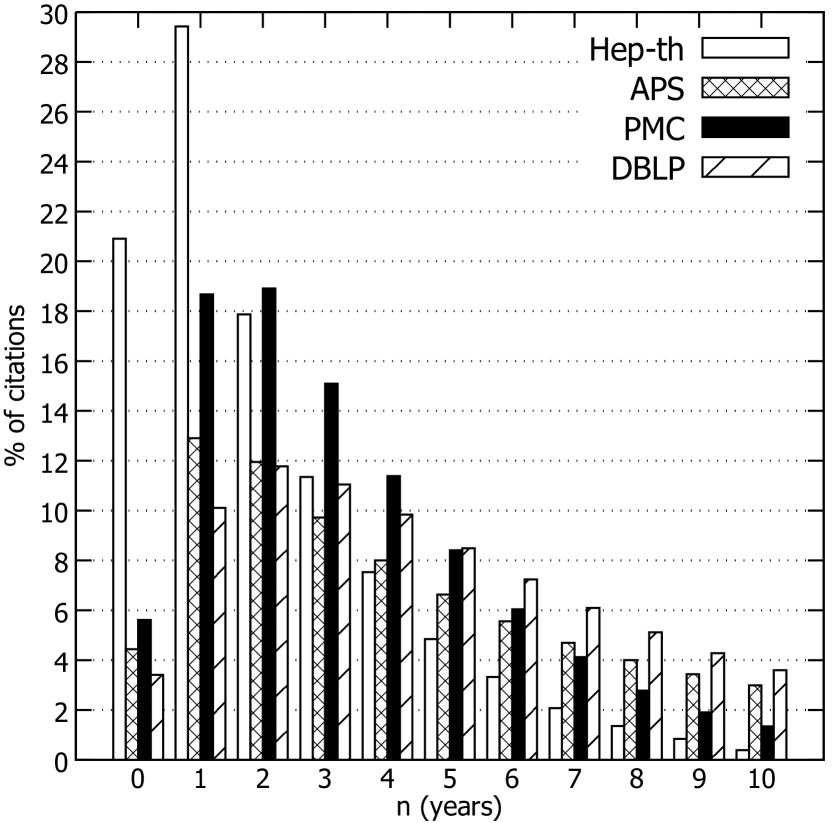
(a)

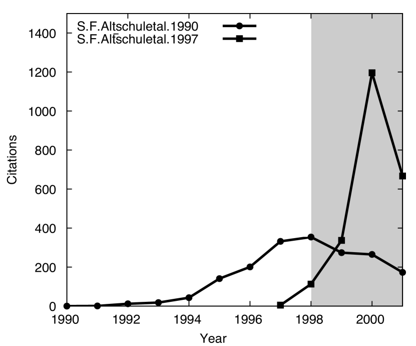
(b)

Figure 1: (a) Empirical distribution of the fraction of total citations received by papers $n$ years after their publication ($n\leq 10$), from four citation networks (see Section IV-A) (b) A comparative yearly citation count of two papers.

As a motivating example for the importance of short-term impact, examine the case of two seminal papers in the bioinformatics literature. The first, published in 1990, introduces the initial version of the popular BLAST alignment algorithm, while the second, published in 1997, presents an improved alignment algorithm by the same team. Figure 1(b) comparatively illustrates their yearly citation counts. Now, consider a bioinformatics researcher living in the year 1998. At that point in time, the older paper has a higher citation count. However, the newer paper is clearly more popular as it has a greater short-term impact, evidenced by the number of citations it collects in the next three years (highlighted in the figure). The 1998 researcher would benefit from being able to identify the newer paper as potentially having a higher short-term impact.

Consider the state of the citation matrix at present time $n$. Given a time horizon of $\tau$, the short-term impact (STI) ${f}_{i}$ of a paper $i$ (where $i\leq n$) is defined as the number of future citations, i.e., those it would receive in the time period $(n,n+\tau]$:

$${f}_{i}=\sum_{j=n+1}^{n+\tau}{C}^{(n+\tau)}_{i,j}.$$

Some observations are in order. First, the time horizon $\tau$ is a user-defined parameter that specifies how long in the future one should wait for citations to accumulate. An appropriate value may depend on the typical duration of the research cycle (preparation, peer-reviewing, and publishing) specific to each scientific discipline. Second, it is important to emphasize that STI can only be computed in retrospect; at current time $t_{N}$, the future citations are not yet observed. Thus, any method that seeks to identify papers with high STI has to employ a mechanism to account for the unobserved future citations.

With these remarks in mind and similar to prior work [4, 5, 12], we study the following problem.

Problem 1.

Given the state ${\bm{C}}^{(n)}$ of the citation network at current time $n$, return a ranking of papers such that it matches their ranking by short-term impact ${\bm{f}}$ for a given time horizon $\tau$.

III Approach

We first overview our approach presenting insight about how to rank based on STI. Then, we describe a useful tool, which we later exploit.

III-A Overview

To rank by short term impact without knowing the future, one needs to introduce assumptions about how the citation network evolves. In this work, we assume that the PageRank vector at time $t\geq n$ indicates the chance the papers will get cited at future time $t+1$. This defines a mechanism, where a random researcher explores literature. While reading a paper, the researcher may choose with probability $\alpha$ to further read one of the paper’s references, or pick another paper at random from some prior (teleport) probability. So the probability of a paper $i$ receiving a citation from a random researcher at time $t+1$ is proportional to their PageRank ${v}^{(t)}_{i}$ at time $t$, which satisfies:

$${\bm{v}}^{(t)}=\alpha{\bm{S}}^{(t)}{\bm{v}}^{(t)}+(1-\alpha){\bm{u}}^{(t)},$$

where ${\bm{S}}^{(t)}$ is the stochastic matrix and ${\bm{u}}^{(t)}$ is the teleport vector at $t$.

The short-term impact of a paper is the sum of citations it will receive at each time $t$ between $n+1$ and $n+\tau$. Let us further assume that each paper in the future (after current time $n$) makes the same number of citations. So, under our assumptions, the number of future citations ${f}_{i}$ a paper $i$ receives is proportional to:

$${f}_{i}\propto\sum_{t=0}^{\tau-1}{v}_{i}^{(n+t)}.$$

For the purposes of ranking, the scale of individual ${f}_{i}$ does not matter. Therefore, to rank by STI we would like to estimate the following vector:

$${\bm{y}}=\sum_{t=0}^{\tau-1}{\bm{v}}_{[n]}^{(n+t)},$$ (3)

i.e., the sum at each future timestamp of the PageRank of the present $n$ papers.

In Equation 3, each PageRank vector ${\bm{v}}_{[n]}^{(n+t)}$ is a random vector under the aforementioned citation network growth process, and its value depends on the values of the PageRank vector at previous times. Therefore, one way to estimate the mean of ${\bm{y}}$ is with Markov Chain Monte Carlo methods to draw samples from the probability distribution of ${\bm{y}}$. This however is costly, as each sample requires the computation of $\tau$ PageRank vectors for a large citation network with at least $n$ nodes.

We propose a different approach. We start by assuming that the future citation matrix and thus ${\bm{S}}^{(n+\tau)}$ is known. Conditional to ${\bm{S}}^{(n+\tau)}$, the PageRank vector ${\bm{v}}_{[n]}^{(n+t)}$ become independent. We then apply a mechanism to rewrite Equation 3 so that it can be computed with a single PageRank computation. This rewriting now has quantities derived from the ${\bm{S}}^{(n+\tau)}$ matrix. At the final step, we estimate these quantities from the current (at time $n$) state of the network, and compute the rewritten Equation 3.

We next describe the mechanism that allows us to rewrite Equation 3 as a single PageRank computation.

III-B The Contraction Mechanism

Consider a network of $n+1$ nodes, where the $(n+1)$-th node has no incoming edges. Its stochastic matrix ${\bm{S}}$ can be written as the following block matrix:

$${\bm{S}}=\begin{pmatrix}{\bm{S}}_{[n]}&{S}_{[n],n+1}\\ {\bm{0}}^{\intercal}&0\end{pmatrix},$$

where ${\bm{S}}_{[n]}$ is the submatrix of ${\bm{S}}$ that contains the first $n$ rows and columns, vector ${S}_{[n],n+1}$ is the first $n$ rows of the $(n+1)$ column of ${\bm{S}}$ and indicates the outgoing connections of node $n+1$, and ${\bm{0}}$ is the zero vector (here of size $n$).

Contraction provides the means to compute the PageRank vector for stochastic matrix ${\bm{S}}$ by contracting node $n+1$ and computing a PageRank vector for ${\bm{S}}_{[n]}$. To account for the contribution from node $n+1$ to its connections, the teleport probabilities to them are appropriately adjusted.

Theorem 1.

Let ${\bm{v}}=({\bm{v}}_{[n]}\ {v}_{n+1})^{\intercal}$ denote the PageRank vector for stochastic matrix ${\bm{S}}=\begin{pmatrix}{\bm{S}}_{[n]}&{S}_{[n],n+1}\\ {\bm{0}}^{\intercal}&0\end{pmatrix}$ with respect to teleport vector ${\bm{u}}=({\bm{u}}_{[n]}\ {u}_{n+1})^{\intercal}$. Define the adjusted teleport vector $\mathring{{\bm{u}}}_{[n]}={\bm{u}}_{[n]}+\alpha{u}_{n+1}{S}_{[n],n+1}$. Then, the normalized ${\bm{v}}_{[n]}$ is the PageRank for matrix ${\bm{S}}_{[n]}$ with respect to the normalized $\mathring{{\bm{u}}}_{[n]}$, i.e., it holds that:

$$\frac{1}{|{\bm{v}}_{[n]}|}{\bm{v}}_{[n]}=\frac{\alpha}{|{\bm{v}}_{[n]}|}{\bm{S}}_{[n]}{\bm{v}}_{[n]}+\frac{1-\alpha}{|\mathring{{\bm{u}}}_{[n]}|}\mathring{{\bm{u}}}_{[n]}.$$

Moreover, ${v}_{n+1}=(1-\alpha){u}_{n+1}$ and $|{\bm{v}}_{[n]}|=|\mathring{{\bm{u}}}_{[n]}|=1-{v}_{n+1}$.

Proof.

Observe that the $x$-th power ($x\geq 1$) of ${\bm{S}}$ is given by:

$${\bm{S}}^{x}=\begin{pmatrix}{\bm{S}}_{[n]}^{x}&{\bm{S}}_{[n]}^{x-1}{S}_{[n],n+1}\\ {\bm{0}}^{\intercal}&0\end{pmatrix}.$$

From Equation 2, we have:

$$\begin{pmatrix}{\bm{v}}_{[n]}\\ {v}_{n+1}\end{pmatrix}= \ (1-\alpha)\begin{pmatrix}{\bm{u}}_{[n]}\\ {u}_{n+1}\end{pmatrix}$$

$$+ \ (1-\alpha)\sum_{x=1}^{\infty}\alpha^{x}\begin{pmatrix}{\bm{S}}_{[n]}^{x}&{\bm{S}}_{[n]}^{x-1}{S}_{[n],n+1}\\ {\bm{0}}^{\intercal}&0\end{pmatrix}\begin{pmatrix}{\bm{u}}_{[n]}\\ {u}_{n+1}\end{pmatrix}.$$

From the bottom row, we immediately get ${v}_{n+1}=(1-\alpha){u}_{n+1}$, while $|{\bm{v}}_{[n]}|=1-{v}_{n+1}$.

We expand the top row to derive:

$${\bm{v}}_{[n]}= \ (1-\alpha){\bm{u}}_{[n]}+(1-\alpha)\sum_{x=1}^{\infty}\alpha^{x}{\bm{S}}_{[n]}^{x}{\bm{u}}_{[n]}$$

$$\ +(1-\alpha)\sum_{x=1}^{\infty}\alpha^{x}{u}_{n+1}{\bm{S}}_{[n]}^{x-1}{S}_{[n],n+1}$$

$$= \ (1-\alpha){\bm{u}}_{[n]}+(1-\alpha)\sum_{x=1}^{\infty}\alpha^{x}{\bm{S}}_{[n]}^{x}{\bm{u}}_{[n]}$$

$$\ +(1-\alpha)\alpha{u}_{n+1}{S}_{[n],n+1}$$

$$\ +(1-\alpha)\alpha\sum_{x=1}^{\infty}\alpha^{x}{u}_{n+1}{\bm{S}}_{[n]}^{x}{S}_{[n],n+1}$$

$$= \ (1-\alpha)({\bm{u}}_{[n]}+\alpha{u}_{n+1}{S}_{[n],n+1})$$

$$\ +(1-\alpha)\sum_{x=1}^{\infty}\alpha^{x}{\bm{S}}_{[n]}^{x}({\bm{u}}_{[n]}+\alpha{u}_{n+1}{S}_{[n],n+1})$$

$$= \ (1-\alpha)\mathring{{\bm{u}}}_{[n]}+(1-\alpha)\sum_{x=1}^{\infty}\alpha^{x}{\bm{S}}_{[n]}^{x}\mathring{{\bm{u}}}_{[n]}.$$

By introducing ${\bm{M}}_{[n]}=(1-\alpha)\sum_{x=0}^{\infty}\alpha^{x}{\bm{S}}_{[n]}^{x}$, the previous equation is written as ${\bm{v}}_{[n]}={\bm{M}}_{[n]}\mathring{{\bm{u}}}_{[n]}$. Multiplying by $1/|\mathring{{\bm{u}}}_{[n]}|$ we get that $\frac{1}{|\mathring{{\bm{u}}}_{[n]}|}{\bm{v}}_{[n]}$ is the PageRank vector for ${\bm{S}}_{[n]}$ with respect to normalized $\mathring{{\bm{u}}}_{[n]}$. It remains to show that $|\mathring{{\bm{u}}}_{[n]}|=|{\bm{v}}_{[n]}|$, which holds because:

$$|\mathring{{\bm{u}}}_{[n]}|= \ |{\bm{u}}_{[n]}|+\alpha{u}_{n+1}\sum_{i=1}^{n}{S}_{i,n+1}=1-{u}_{n+1}+\alpha{u}_{n+1}$$

$$= \ 1-(1-\alpha){u}_{n+1}=1-{v}_{n+1}=|{\bm{v}}_{[n]}|.$$

∎

Contraction can be applied recursively to networks containing multiple nodes that have no incoming edges. Consider a network of $n+m$ nodes, represented by its stochastic matrix ${\bm{S}}$, where its $m$ last nodes have no incoming edges. Given some teleport vector ${\bm{u}}$ and random jump probability $\alpha$, let ${\bm{v}}$ denote the PageRank vector that satisfies ${\bm{v}}=(1-\alpha)\sum_{x=0}^{\infty}\alpha^{x}{\bm{S}}^{x}{\bm{u}}$. The PageRank scores ${\bm{v}}_{[n]}$ of the first $n$ nodes can be computed directly from the PageRank on the stochastic matrix ${\bm{S}}_{[n]}$ with respect to an adjusted teleport vector $\mathring{{\bm{u}}}$, as indicated by the following theorem.

Theorem 2.

Let ${\bm{v}}$ denote the PageRank vector for stochastic matrix ${\bm{S}}=\begin{pmatrix}{\bm{S}}_{[n]}&{\bm{S}}_{[n],[-m]}\\ {\bm{0}}_{(m\times n)}&{\bm{0}}_{(m\times m)}\end{pmatrix}$ with respect to teleport vector ${\bm{u}}$ and random jump probability $\alpha$. Define the adjusted teleport vector $\mathring{{\bm{u}}}_{[n]}={\bm{u}}_{[n]}+\alpha\sum_{i=1}^{m}{u}_{n+i}{S}_{[n],n+i}$. Then it holds that:

$$\frac{1}{|{\bm{v}}_{[n]}|}{\bm{v}}_{[n]}=\frac{\alpha}{|{\bm{v}}_{[n]}|}{\bm{S}}_{[n]}{\bm{v}}_{[n]}+\frac{1-\alpha}{|\mathring{{\bm{u}}}_{[n]}|}\mathring{{\bm{u}}}_{[n]},$$

where $|\mathring{{\bm{u}}}_{[n]}|=|{\bm{v}}_{[n]}|=1-(1-\alpha)\sum_{i=1}^{m}{u}_{n+i}$.

Proof.

Follows from applying Theorem 1 $m$ times. At the first iteration, the adjusted teleport vector is:

$${\bm{u}}_{[n+m-1]}^{(n+m-1)}={\bm{u}}_{[n+m-1]}+\alpha{u}_{n+m}{S}_{[n+m-1],n+m}.$$

At the second iteration:

$${\bm{u}}_{[n+m-2]}^{(n+m-2)}=\ {\bm{u}}_{[n+m-2]}^{(n+m-1)}+\alpha{u}_{n+m-1}{S}_{[n+m-2],n+m-1}$$

$$=\ {\bm{u}}_{[n+m-2]}+\alpha{u}_{n+m}{S}_{[n+m-2],n+m}$$

$$+\alpha{u}_{n+m-1}{S}_{[n+m-2],n+m-1}$$

$$=\ {\bm{u}}_{[n+m-2]}+\alpha\sum_{i=m-1}^{m}{u}_{n+i}{S}_{[n+m-2],n+i}.$$

At the $m$-th iteration, we get ${\bm{u}}_{[n]}^{(n)}=\mathring{{\bm{u}}}_{[n]}$.

Moreover, for each $i$, such that $1\leq i\leq m$, we have ${v}_{n+i}=(1-\alpha){u}_{n+i}$, which means $|{\bm{v}}_{[n]}|=1-\sum_{i=1}^{m}{v}_{n+i}=1-(1-\alpha)\sum_{i=1}^{m}{u}_{n+i}$.

Finally, for each $i$, it holds that $\sum_{j=1}^{n+i}{S}_{j,n+i}=\sum_{j=1}^{n}{S}_{j,n+i}=1$, since node $n+i$ has outgoing edges only to nodes with id not greater than $n$. As a consequence, $|\mathring{{\bm{u}}}_{[n]}|=|{\bm{v}}_{[n]}|$. ∎

In other words, to compute the PageRank w.r.t. ${\bm{S}}$ for the first $n$ nodes, we can use an adjusted teleport vector $\mathring{{\bm{u}}}_{[n]}$ (after normalization) to compute the PageRank w.r.t. ${\bm{S}}_{[n]}$, and then scale the result by $|\mathring{{\bm{u}}}_{[n]}|$.

III-C The AttRank Method

We will apply the contraction idea to compute each future PageRank vector ${\bm{v}}_{[n]}^{(n+t)}$ as a PageRank vector of the current stochastic matrix ${\bm{S}}^{(n)}$, assuming that its future state ${\bm{S}}^{(n+t)}$ is known. Note that to apply the contraction idea, we need to restrict each future paper $i$ to cite no other future paper $j$ ($n<j<i$), i.e., citations only come for papers already published until current time $n$. This restriction only affects the PageRank values of the future papers, which however we do not need to rank.

Note that for any time $n+t$ where $t>0$, the first $n$ rows and columns of the stochastic matrix ${\bm{S}}^{(n+t)}$ remain constant, and we denote ${\bm{S}}\equiv{\bm{S}}_{[n]}^{(n+t)}$. From Theorem 2 we have:

$$\frac{1}{|{\bm{v}}_{[n]}^{(n+t)}|}{\bm{v}}_{[n]}^{(n+t)}=\frac{\alpha}{|{\bm{v}}_{[n]}^{(n+t)}|}{\bm{S}}{\bm{v}}+\frac{1-\alpha}{|{\bm{v}}_{[n]}^{(n+t)}|}\mathring{{\bm{u}}}_{[n]}^{(n+t)}.$$

Defining ${\bm{M}}=(1-\alpha)\sum_{x=0}^{\infty}\alpha^{x}{\bm{S}}^{x}$, we rewrite the previous equation in the closed form of Equation 2:

$${\bm{v}}_{[n]}^{(n+t)}={\bm{M}}\mathring{{\bm{u}}}_{[n]}^{(n+t)}.$$

From the definition of STI, we derive:

$${\bm{y}}=\sum_{t=0}^{\tau-1}{\bm{v}}_{[n]}^{(n+t)}={\bm{M}}\sum_{t=0}^{\tau-1}\mathring{{\bm{u}}}_{[n]}^{(n+t)},$$

where $\mathring{{\bm{u}}}_{[n]}^{(n+t)}={\bm{u}}_{[n]}^{(n+t)}+\alpha\sum_{i=1}^{m}{u}_{n+i}^{(n+t)}{S}_{[n],n+i}^{(n+t)}$.

For convenience, we further assume that the teleport vector for the first $n$ papers is the same at each time $n+t$, and we denote it as ${\bm{u}}\equiv{\bm{u}}_{[n]}^{(n+t)}$. We thus split the adjusted teleport vectors into a non-time-dependent component and a time-dependent component: $\mathring{{\bm{u}}}_{[n]}^{(n+t)}={\bm{u}}+{\bm{w}}_{[n]}^{(n+t)}$. Summing the time-dependent components for $0\leq t\leq\tau-1$, we introduce:

$${\bm{w}}\equiv\sum_{t=0}^{\tau-1}{\bm{w}}_{[n]}^{(n+t)}=\alpha\sum_{t=0}^{\tau-1}\sum_{i=1}^{t}{u}_{n+i}{S}^{(n+t)}_{[n],n+i}.$$

Then, the STI can be expressed as:

$${\bm{y}}={\bm{M}}(\tau{\bm{u}}+{\bm{w}}),$$

meaning that $\hat{{\bm{y}}}\equiv\frac{{\bm{y}}}{|{\bm{y}}|}$ can be computed as the PageRank vector of matrix ${\bm{S}}$ with respect to teleport vector $\frac{\tau}{|{\bm{y}}|}{\bm{u}}+\frac{1}{|{\bm{y}}|}{\bm{w}}$. Introducing coefficients $\alpha,\beta,\gamma\in[0,1]$, such that $\alpha+\beta+\gamma=1$, we can write STI in a general form:

$$\hat{\bm{y}}=\alpha{\bm{S}}\hat{\bm{y}}+\beta\hat{\bm{w}}+\gamma\hat{\bm{u}},$$ (4)

where $\hat{\bm{w}}$ and $\hat{\bm{u}}$ are the normalized vectors of ${\bm{w}}$ and ${\bm{u}}$, respectively.

Attention. Because the time-dependent vector ${\bm{w}}$ is determined by quantities of future states ${\bm{S}}^{(n+t)}$, we need to estimate it from the known current state ${\bm{S}}$. A simple way is instead of going $\tau$ time steps in the future, to go $y$ time steps in the past. Assuming teleport probabilities ${u}_{n+t}$ for future papers are equal, we estimate:

$$\tilde{\bm{w}}\propto\sum_{t=0}^{y-1}\sum_{i=0}^{t}{S}_{[n],n-i}=\sum_{i=0}^{y-1}(y-i){S}_{[n],n-i}.$$ (5)

We call this estimated vector $\tilde{\bm{w}}$ the attention vector, because for each paper $i$, it computes a weighted count of its citations from the $y$ most recent papers, i.e., its recent attention $\tilde{w}_{i}\propto y{S}_{i,n}+(y-1){S}_{i,n-1}+\dots+{S}_{i,n-y+1}$.

Note that if ${\bm{u}}$ represents the regular teleport probability vector, the attention vector ${\bm{w}}$ introduces yet another teleport probability, suggesting that researchers tend to to read and cite currently trending papers. i.e., papers that have recently received significant attention from the scientific community. To investigate this hypothesis, we explore four citation networks (as per the default experimental configuration discussed in Section IV-A), and count how many top-$100$ papers were recently popular, based on STI (i.e., were among the top cited in the past $5$ years). As we see in Table I, roughly half of the top-$100$ papers were, indeed, recently popular. This observation validates our assumption that the level of attention a paper has recently attracted is indicative of its ability to attract citations in the short-term.

TABLE I: Recently popular papers in top-$100$ (accord. to STI)

Dataset	hep-th	APS	PMC	DBLP
Recently Popular	$41$	$54$	$54$	$63$

Attention, however, is not the only mechanism that governs which papers researchers read. Naturally, researchers may read a paper cited in the reference list of another paper. Moreover, similar to previous work [4, 11], we assume that researchers also read recently published papers. Specifically, we capture the recency of a paper $i$ using a score that decays exponentially based on the paper’s age:

$${u}_{i}=ce^{\eta\cdot(n-i)},$$ (6)

where $n$ is the current time, $i<n$ denotes the publication time of paper $i$, hyperparameter $\eta$ is a negative constant (as $n-i\geq 0$), and $c$ is normalization constant so that $|{\bm{u}}|=1$. To calculate a proper $\eta$ value, a similar procedure like the one used in [11] can be followed (see also Section IV-B).

AttRank. We refer to the ranking approach based on Equations 4, 5, and 6 as AttRank. Note that Eq. 4 combines three mechanisms. Specifically, we assume that a researcher may read a paper for one of the following reasons: the paper gathered attention recently, the paper was recently published, or the paper was found in another paper’s reference list. We model this behavior with the following random process. A researcher, after reading paper $i$, chooses to read any other paper from $i$’s reference list, with probability $\alpha$. With probability $\beta$ she chooses a paper based on its attention. This behavior essentially makes recently rich papers even richer, and is reminiscent of a time-restricted preferential attachment mechanism of the Barabási-Albert model of network growth [13]. Finally, with probability $\gamma$ she chooses any paper with a preference towards recently published ones.

Two special values for coefficient $\beta$ are worth mentioning. First, observe that when $\beta=0$, a setting we call NO-ATT (for no attention), the model becomes similar to time-aware methods that address the inherent bias against new papers in citation networks (see also Section V, and [12] for a thorough coverage of such approaches). Note that additionally setting $\eta=0$ in Eq. 6 recovers PageRank. Second, when $\beta=1$, a setting we call ATT-ONLY (for attention only), AttRank is solely based on the attention mechanism, assuming that the recent citation patterns will persist exactly in the near future. To the best of our knowledge, ATT-ONLY has not been considered in the literature as a means to estimate the short-term impact of a paper. As we show in Section IV, attention alone is a powerful mechanism, often more effective than existing approaches. However, $\beta=1$ is never the optimal setting; it is always better to consider attention in combination with the other two citation mechanisms.

Equation 4 describes an iterative process for estimating STI vector: starting with a random value, at each step update the vector with the right hand side of the equation. This process is repeated until the values converge. The following theorem, ensures that convergence is achievable.

Theorem 3.

The iterative process defined by Eq. 4 converges.

Proof.

We can rewrite Equation 4 in matrix form as:

$$\hat{\bm{y}}={\bm{R}}\hat{\bm{y}}$$ (7)

where ${\bm{R}}$ is a matrix satisfying:

$${R}_{i,j}=\alpha{S}_{i,j}+\beta\hat{w}_{i}+\gamma\hat{u}_{i}$$ (8)

In other words, matrix ${\bm{R}}$ is a modified citation matrix, artificially expanded with directed edges from any node to any other in the network. It is easy to see that it is a stochastic matrix where each column sums to 1. Moreover, it satisfies the conditions of irreducibility and aperiodicity [15] and thus the iterative process is guaranteed to converge. ∎

IV Evaluation

This section presents a thorough experimental evaluation of our approach for ranking papers based on their short-term impact. Specifically, Section IV-A discusses the experimental setup and evaluation approach taken. Section IV-B investigates the effectiveness of our proposed method and the importance of the attention-based mechanism. Section IV-C compares AttRank with existing approaches from the literature. Finally, Section IV-D discusses the convergence rate of AttRank.

IV-A Experimental Setup

Datasets. We consider four datasets in our experiments:

1. arXiv’s high energy physics (hep-th) collection, which was provided by the 2003 KDD cup. This collection consists of approximately 27,000 papers with 350,000 references, written by 12,000 authors from 1992 to 2003.

2. A collection of papers provided by the American Physical Society (APS), which contains about 500,000 papers with 6 million references, written by about 389,000 authors from 1893 to 2014.

3. A collection of open access papers from pubmed central (PMC), which consists of about 1 million papers with 665,000 references, written by 5 million authors, from 1896 to 2016.

4. A collection of about $3$ million papers and $25$ million references, written by more than $1.7$ million authors, from the computer science domain (DBLP), published from 1936 to 2018.

Evaluation Methodology. To evaluate the effectiveness of AttRank in ranking papers based on their short-term impact, we construct a current and a future state of the citation network. We partition each dataset according to time in two parts, each having equal number of papers. We use the older half to construct the current state of the citation network, denoted as ${\bm{C}}^{(n)}$. All ranking methods will be based on this network acting as the “training” subset. We use parts of the newer half to construct the future state of the network, denoted as ${\bm{C}}^{(n+\tau)}$. All ranking methods will be evaluated based on this network acting as the “test” subset.

Specifically, the future state is constructed as follows. We vary the size, in terms of number of papers, of the future state relative to the size of the current state. Thus we do not vary the time horizon $\tau$ directly, but rather the test ratio, which is the relative size of the future with respect to the current network. We consider values for the test ratio among $\{1.2,1.4,1.6,1.8,2.0\}$, where $2.0$ corresponds to using all citations in the dataset to define the future state. In some experiments we fix the test ratio to a default value of $1.6$, meaning that the future state contains $30$% more papers than the current state. Table II presents, for each dataset, the length in years of the time horizon that corresponds to each test ratio value. Note, that the relationship between test ratio and $\tau$ is not linear, due to the non-constant number of published papers per year and the fact that most datasets contain incomplete entries for the last year they include.

TABLE II: Correspondence of the Test Ratio to the Time Horizon

Test	Time Horizon $\tau$ (in years)
Ratio	hep-th	APS	PMC	DBLP
1.2	1	4	1	1
1.4	2	7	2	3
1.6	3	10	2	4
1.8	4	13	3	6
2.0	5	16	3	7

Given the future state of the citation network, we can compute the STI of each paper as per its definition (see Section II). Similar to previous approaches in the literature [11, 4, 5, 12], the ranking of papers based on their STI forms the ground truth. Any paper ranking method is oblivious of the future state ${\bm{C}}^{(n+\tau)}$ of the citation network, and hence the ground truth, and only uses the current state ${\bm{C}}^{(n)}$ to derive a ranking. To quantify the effectiveness of a method, we compare its produced ranking to the ground truth, using the following two measures:

• Spearman’s $\rho$ [16] is a non-parametric measure of rank correlation. It is based on the $L1$ distance of the ranks of items in two ranked lists and provides a quantitative measure to compare how similar these lists are. Its values range from $-1$ to $1$ with $1$ denoting perfect correlation, $-1$ denoting perfect negative correlation and $0$ denoting no correlation.

• Normalized Discounted Cumulative Gain at rank $k$ (nDCG@$k$) is a rank-order sensitive metric. The discounted cumulative gain (DCG) at rank $k$ of a paper is computed as $\text{DCG}@k=\sum_{i=1}^{k}{\frac{rel(i)}{\log_{2}(i+1)}}$, where $rel(i)$ is the ground truth score, i.e., the short-term impact, of the paper that appears at the $i$-th position on the method’s ranking. The nDCG@$k$ is the paper’s DCG divided by the ideal DCG, achieved when the method’s ranking coincides with the ground truth. In our evaluation, we consider values of $k$ among $\{5,10,50,100,500\}$, with $k=50$ being used as a default value.

Spearman’s $\rho$ calculates an overall similarity of the given ranking with the ground truth ranking. In contrast, nDCG@$k$ measures the agreement of the two rankings on the top-ranking papers.

IV-B Ranking Effectiveness

TABLE III: AttRank’s parameterization space.

Parameter	min	max	step
$\alpha$	0.0	0.5	0.1
$\beta$	0.0	1.0	0.1
$\gamma$	0.0	0.9	0.1
$y$	1	5	1

In this section, we investigate AttRank’s effectiveness for the default experimental setting (test ratio equal to $1.6$), while varying its parameters, $\alpha,\beta,\gamma$, and the number $y$ of past years used to calculate the attention of a paper. The range of values tested are shown in Table III. For each metric, we discuss AttRank’s parameterization that achieves the best ranking effectiveness.

First, however, we discuss how we set the value of the exponential factor $\gamma$ of Equation 6. We follow a similar approach as the one used in [11]. For each dataset, we use an exponential function of the form $e^{\widetilde{\gamma}y}$, to fit the tail of the distribution of the random variable $Y$ that models the probability of an article being cited $n$ years after its publication. Figure 1(a) illustrates the empirical probability distribution for each dataset. The factor $\widetilde{\gamma}$ of the fitting function is used as the $\gamma$ value. Following this procedure, we calculate $\gamma=-0.48$ for hep-th, $\gamma=-0.12$ for APS and $\gamma=-0.16$ for PMC and DBLP.

IV-B1 Effectiveness in terms of Correlation

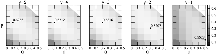
(a) Correlation on the DBLP dataset.

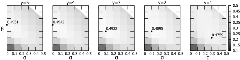
(b) Correlation on the PMC dataset.

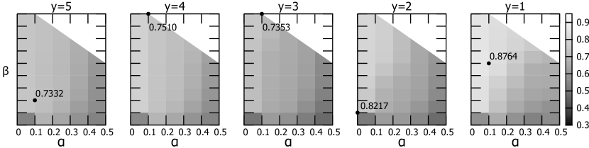
(c) nDCG@50 on the DBLP dataset.

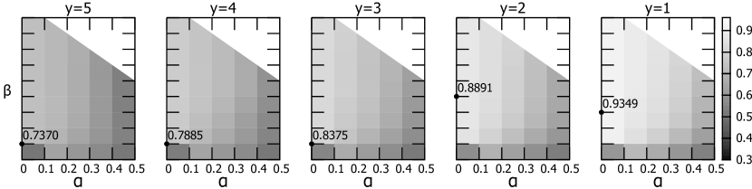
(d) nDCG@50 on the PMC dataset.

Figure 2: Heatmaps depicting the effect of the parameterization of AttRank to its effectiveness in terms of the correlation and nDCG@50 metrics, for the DBLP and PMC datasets. The best value achieved for each metric is also depicted.

In this experiment, we measure the ranking effectiveness of AttRank, in terms of Spearman’s $\rho$ to the ground truth ranking by STI. We can visualize the effectiveness of each tested parameterization as a heatmap over the $\alpha$–$\beta$ space for different values of $y$. Indicatively, we show the heatmaps, for the various parameter settings on DBLP and PMC in in Figures 2(a) and 2(b), respectively. The heatmaps show the results varying parameters $\alpha$, and $\beta$; parameter $\gamma$ is implied since $\alpha+\beta+\gamma=1$. We expect that as $\alpha$ increases, AttRank simulates researchers that predominantly prefer reading papers from reference lists and rarely choose papers based on their age, or on whether they have been recently popular. Thus, as $\alpha$ increases, AttRank gradually reduces to simple PageRank, with a small probability of random jumps. Since references are made only to papers published in the past, researchers increasingly arrive at older papers when following references with high probability. As a result, for large $\alpha$ values, AttRank promotes older papers and, thus, its correlation to the ground truth is expected to drop. Most importantly, the heatmaps validate the role of the attention scores, since for $\beta=0$ (NO-ATT) we observe significantly lower correlations (notice the darker color on the bottom left corner of the heatmaps). Similarly, lower correlations were observed when $\beta=1$ (ATT-ONLY).

From the produced correlation scores, we firstly gather that AttRank correlates at least moderately to the ground truth ranking for all datasets in its best setting (i.e., $\rho>0.49$). Further, we observe that the optimal value for the number of past years $y$, used to calculate the attention score is $y=3$ and $y=4$ on DBLP and PMC, respectively, while it’s $y=3$ on APS, and $y=1$ on hep-th.

Interestingly, the first three datasets follow relatively similar citation patterns (see Figure 1(a)), with papers having a citation peak at $2-3$ years after their publication, while hep-th shows quicker citation peaks. Intuitively then, it makes sense to use a smaller value of $y$ to calculate attention scores for hep-th. Since its research trends may change faster, a larger time window to calculate the attention would reflect past research trends, and not current ones. On APS, PMC, and DBLP, in contrast, papers gather citations at a slower rate, thus a larger $y$ value is more likely to reflect current research preferences.

Based on these experiments, we also identify the optimal parameterization that achieves maximum correlation per dataset. We find the best settings of {$\alpha$,$\beta$,$\gamma$,$y$} at {$0.3,0.4,0.3,1$} for hep-th ($\rho=0.6519$), {$0.3,0.3,0.4,3$} for APS ($\rho=0.6295$), {$0.0,0.4,0.6,4$} for PMC ($\rho=0.494$), and {$0.2,0.4,0.4,3$} for DBLP ($\rho=0.6316$). To illustrate the significance of the attention mechanism, compare these results to the maximum values for $\beta=0$ (NO-ATT). These are $0.56$, $0.581$, $0.411$, and $0.529$ for hep-th, APS, PMC, and DBLP, respectively. Accordingly, for $\beta=1$, these values are $0.615$, $0.537$, $0.444$, $0.571$.

IV-B2 Effectiveness in terms of nDCG@50

We repeat the effectiveness analysis, this time considering the nDCG@50 metric. Indicatively, we present the heatmaps for DBLP and PMC in Figures 2(c) and 2(d), respectively. An interesting observation is that with regards to only capturing the papers with the highest short-term impact, smaller time windows on which the attention scores are calculated seem to be more suitable. We observe that as $y$ increases, the overall nDCG values decrease (notice the darker hues when $y$ increases). We expect that by further increasing $y$, the nDCG would further drop. This is because by increasing the time window on which we calculate the attention we, re-introduce the inherent age bias of citation networks, and the papers with the highest attention scores no longer reflect current research trends. The same observation holds for increased values of $\alpha$ when $y>1$. As $\alpha$ increases, the PageRank component dominates AttRank, giving advantage to older papers that are not necessarily at the current focal point of research. This observation is evident from the darker hues on the heatmaps for values of $\alpha$ close to $0.5$.

Finally, we determine the parameterization that achieves the best nDCG@$50$ per dataset. We find the best settings of parameters {$\alpha$,$\beta$,$\gamma$,$y$} at {$0.0$,$0.4$,$0.6$,$1$} for hep-th ($nDCG=0.8930$), {$0.3$,$0.5$,$0.2$,$3$} for APS ($nDCG=0.7293$), {$0.0$,$0.3$,$0.7$,$1$} for PMC ($nDCG=0.9349$) and {$0.1$, $0.5$, $0.4$, $1$} for DBLP ($nDCG=0.8764$). As before, we observe that the attention vector plays a non-negligible role in achieving the maximum nDCG on all datasets (i.e., $\beta>0$). Indicatively, the maximum nDCG@$50$ values for $\beta=0$ are $0.653$, $0.635$, $0.6$, and $0.683$ for hep-th, APS, PMC, and DBLP, respectively. Accordingly, for $\beta=1$ these values are $0.89$, $0.71$, $0.930$, $0.862$.

IV-C Comparative Evaluation

In this section, we compare AttRank to existing approaches for impact-based paper ranking. Based on a recent experimental evaluation [12], we select the five methods found to be most effective in ranking by short-term impact.

• CiteRank (CR). This PageRank-based method calculates the “traffic” towards papers by researchers that prefer reading recently published papers when performing random jumps [4]. It uses parameters $\alpha\in(0,1)$ and $\tau_{dir}\in(0,\infty)$, where $\alpha$ models the probability with which researchers follow references from papers they read and $\tau_{dir}$ models an aging factor, which determines the papers which random researchers are more likely to select when performing random jumps. In the original work, their optimal settings are found for $\{\alpha,\tau_{dir}\}$ set to $\{0.48,1\}$, $\{0.5,2.6\}$,$\{0.31,1.6\}$,$\{0.55,8\}$.

• FutureRank (FR). This method is based on PageRank and HITS [17]. It applies mutual reinforcement from papers to authors and vice versa, while additionally using time-based weights to promote recently published papers [11]. It uses four parameters: $\alpha,\beta,\gamma\in(0,1)$, and $\rho\in(-\infty,0)$. Parameter $\alpha$ is taken from PageRank, $\beta$ is the coefficient of an author-based score vector, and $\gamma$ is the coefficient of time-based weights. These weights depend on $\rho$, which modifies an exponentially decreasing function. In the original work the optimal settings of $\{\alpha,\beta,\gamma,\rho\}$ are $\{0.4,0.1,0.5,-0.62\}$, and $\{0.19,0.02,0.79,-0.62\}$.

• Retained Adjacency Matrix (RAM). This citation count variant uses a citation age-weighted adjacency matrix [5]. It uses a parameter $\gamma\in(0,1)$ as the base of an exponential function, to modify citation weights, based on their age. The authors find $\gamma\in\{0.3,0.6,0.71\}$ as as the optimal settings.

• Effective Contagion Matrix (ECM). This method, based on Katz centrality, operates over a citation age-weighted adjacency matrix [5] and calculates weights of citation chains. It uses parameters, $\alpha,\gamma\in(0,1)$, where $\gamma$ is taken from RAM, and $\alpha$ is used to decrese citation chain weights as they increase in length. In the original work, the authors find the best settings of $\{\alpha,\gamma\}$ to be $\{0.1,0.3\}$ or $\{0.007,0.71\}$.

• WSDM cup’s 2016 winner (WSDM). We consider the winning solution [18] of a scholarly article ranking challenge. This method uses three bipartite networks (papers-authors, papers-papers, and papers-venues). It calculates paper scores by aggregating scores propagated to papers by other papers, by their authors, and their venues, additionally using scores based on paper in- and out-degrees. Paper scores are calculated iteratively, based on a fixed small number of iterations. The method uses parameters $\alpha,\beta\in\mathbb{R}$, as coefficients of each paper’s in- and out-degree, to calculate paper scores, and the number of iterations, $i$. The authors use $\{\alpha,\beta\}=\{1.7,3\}$ in their work and set $i\in\{4,5\}$.

TABLE IV: Parameterization space of competitors.

Method	Parameter	min	max	step
CR	$\alpha$	0.1	0.7	0.2
	$\tau_{dir}$	2	10	2
FR	$\alpha$	0.1	0.5	0.1
	$\beta$	0.0	0.9	0.1
	$\gamma$	0.0	0.9	0.1
	$\rho$	-0.82	-0.42	0.2
RAM	$\gamma$	0.1	0.9	0.1
ECM	$\alpha$	0.1	0.5	0.1
	$\gamma$	0.1	0.5	0.1
WSDM	$\alpha$	1.1	2.3	0.3
	$\beta$	1	5	1
	$i$	4	5	1

The optimal parameterization for the competitors is presented in each work. However, these suggested values result from the use of particular datasets and specific experimental settings, which differ among works. Therefore, in our evaluation, we extensively tuned all competitors, to ensure a fair comparison of their effectiveness in ranking based on STI. Table IV presents the examined parameter sets. In total, we used $20$ different settings for CR, $120$ settings for FR, $9$ settings for RAM, $25$ settings for ECM, and $50$ settings for WSDM. Note, that since WSDM requires venue data, we ran this method only on the PMC and DBLP datasets, for which this data was available. Further, we ran all iterative methods until the convergence error drops below $10^{-12}$, to ensure that all scores approach their final values and further iterations are not expected to change the ranking of papers.

In addition to these existing approaches, we also consider two variants of AttRank that better demonstrate the effect of the attention mechanism. The first, denoted as NO-ATT, removes the attention mechanism in AttRank, i.e., sets $\beta=0$. Conversely, the second, denoted ATT-ONLY, considers only the attention mechanism in AttRank, i.e., sets $\beta=1$.

Figure 3: Effectiveness of all methods in terms of correlation. The x-axis represents the varying test ratio.

IV-C1 Effectiveness in terms of Correlation

In this experiment, we measure the correlation of each method’s ranking to that of the ground truth. We vary the test ratio of the size of networks according to Section IV-A. For each dataset and test ratio, we choose the parameterization with the best correlation. Figure 3 presents the results.

We observe that AttRank’s ranking better correlates to the ground truth ranking, compared to all competitors on all settings for the hep-th, APS, and DBLP datasets. In particular, AttRank increases correlation by up to $0.055$ units on hep-th, by up to $0.057$ on APS, and by up to $0.079$ on DBLP with respect to the best competitor. Further, on most settings AttRank correlates better to the ground truth ranking on PMC, by up to $0.027$, compared to the best competitor, while marginally losing to FR on two settings (the correlation values observed differ by $<0.01$). It is worth highlighting that FR achieves such a good correlation only for PMC; in the other datasets, it is outperformed by other existing methods. In contrast, AttRank is robust across datasets and settings with a large correlation gain over all competitors (except FR in PMC).

Our method’s performance can be attributed to the fact that, compared to the time-aware competitors, it does not simply promote papers recently cited, or recently published. Instead, because of the attention mechanism, it heavily promotes well-cited, recent papers, compared to lesser cited recent papers. As discussed in Section III, recently popular papers indeed remain popular. Moreover, our method promotes older papers that are still heavily cited. The importance of the attention mechanism is illustrated by the fact that in two datasets ATT-ONLY outperforms existing methods. Turning off attention completely, i.e, the NO-ATT method, results in subpar performance, except in one dataset. Most importantly, in all cases, the effectiveness is increased when the attention mechanism is balanced with the other mechanisms in AttRank.

Figure 4: Effectiveness of all methods in terms of nDCG@50. The x-axis represents the varying test ratio.

IV-C2 Effectiveness in terms of nDCG

In this section, we measure the nDCG achieved by each method with regards to the ground truth. We conduct two experiments: in the first, we set $k=50$ as the cut-off rank when computing nDCG, varying the test ratio. In the second experiment we use the default test ratio (at $1.6$) and measure nDCG varying $k$.

Figure 4 presents the results varying the test ratio. For each setting, we select the parameterization of each method that gives the best nDCG@$50$ value. In general, as we look further into the future, i.e., increase the test ratio, the ranking accuracy of all methods drops; the effect is more pronounced in the APS dataset, and less in hep-th. In all cases, AttRank outperforms all competitors, except for one setting on DBLP (for $n=1.2$, it marginally loses to ECM, with a difference of $<0.001$). In particular, our method improves nDCG@$50$ by up to $0.017$ units on hepth, $0.018$ on APS, $0.0156$ on PMC, and $0.0173$ on DBLP, compared to the best existing method. It is worth mentioning that the best existing method varies across datasets, being either RAM or ECM.

Figure 5 presents the results varying $k$ for a test ratio of $1.6$. For each setting, we select the parameterization of each method that gives the best nDCG@$k$ value. In general we observe that AttRank is at least on par, and mostly outperforms all rivals on all datasets, with the sole exception of nDCG@$5$ on APS (the measured difference compared to the best competitor is $0.015$). Specifically, AttRank achieves a higher nDCG value of up to $0.017$ units on hep-th, up to $0.013$ units on APS (except nDCG@$5$), up to $0.0019$ on PMC, and up to $0.01$ units on DBLP. Additionally, for small values of $k$ ($k=\{5,10\}$) AttRank achieves nDCG values close to $1$ on two out of four datasets (hep-th and PMC). The best competitors are again RAM and ECM, depending on the dataset.

Regarding the special cases of AttRank, we observe in both Figures 4 and 5, that excluding attention (NO-ATT) results in a significant drop in nDCG. On the other hand, attention alone (ATT-ONLY) outperforms most existing methods except in APS. As also observed in the case of Figure 3, carefully balancing the mechanisms in AttRank leads to a considerable improvement in ranking accuracy.

Figure 5: Effectiveness of all methods in terms of nDCG@$k$ on the default test ratio. The x-axis represents the varying value of $k$.

IV-D Convergence of AttRank

AttRank involves an iterative process, similar to PageRank, to compute scores for papers. Specifically, we can view AttRank as a PageRank variant, where the random jump vector is replaced by two vectors, the attention-based vector and the publication age-based vector, and thus PageRank’s random jump probability $1-\alpha$ is divided among $\beta,\gamma$ in AttRank. The convergence of AttRank is thus affected by the same factors as PageRank’s; an in-depth discussion of PageRank’s convergence properties can be found in [15]. The most important property is that as $\alpha\to 1$, the convergence rate decreases and more iterations are required.

Following the discussion in Section IV, however, large values of parameter $\alpha$ do not favor ranking based on short-term impact, and AttRank’s optimal effectiveness is always achieved for $\alpha\leq 0.5$. Additionally, as $\alpha\to 0$, AttRank tends to depend increasingly on the sum of the attention- and time-based vectors. Thus, the number of iterations required for convergence decreases, with the limit case $\alpha=0$ requiring a single iteration (i.e., the calculation of the attention- and time-based vectors).

Overall, AttRank is expected to converge faster than PageRank and other variants (PageRank has been used with $\alpha=0.5$ on citation networks [7, 19]). In our experiments, AttRank converges in less than $30$ iterations for hep-th, APS, and DBLP, and less than $20$ iterations for PMC, for $\alpha=0.5$ and a convergence error of $\epsilon\leq 10^{-12}$, with the number of iterations decreasing for smaller values of $\alpha$. Compare this to the maximum required iterations for CR, which are $51$, $46$, $26$, and $47$, for hep-th, APS, PMC, and DBLP, respectively, for $\alpha=0.5$. The corresponding numbers for FR (which did not, in practice, converge under all possible settings) are $35$, $30$, $26$, and $23$, for hep-th, APS, PMC, and DBLP, respectively, and for $\alpha=0.5$.

V Related work

In recent years, various methods have been proposed for quantifying the scientific impact of papers. In the following, we review the most important work, focusing on methods to rank papers by their expected short-term impact. For a thorough coverage of this research area refer to [20, 12].

Basic Centrality Variants. A large number of methods are PageRank adaptations tailored to better simulate the way a random researcher traverses the citation network while reading papers (e.g., [21, 22, 23, 7]). While such approaches modify the random researcher’s behaviour in intuitive ways (e.g., she prefers reading cited papers that are similar to the one she currently reads), they do not address age bias, an important intrinsic issue in citation networks.

Time-Aware Methods. To alleviate age bias, a number of time-aware methods were proposed. These methods introduce time-based weights in the various centrality metric calculations, to favor either recent publications (e.g., [9, 24, 4, 11] or recent citations (e.g., [5]), or citations received shortly after the publication of an article (e.g., [25, 26]).

Although the aforementioned practice has been applied to citation count variants [25, 26, 5] or to Katz centrality [5], most works introduce time-awareness to PageRank adaptations. This is achieved by modifying either the adjacency matrix [9, 24] and/or landing probabilities in the PageRank formula (e.g., [4, 11, 8, 24]). In the former case, the intuition is that the random researcher avoids following references to old papers (with respect to the current time or to the publication year of the citing paper). In the latter case, the random researcher prefers selecting new papers during random jumps.

Time-awareness is shown to improve the accuracy when ranking by short-term impact. However, it fails to differentiate among recent papers favoring all equally. In reality, some papers are fitter than others and will attract more attention. To address this issue, literature proposes using additional information besides the citation network, such as paper metadata and other networks.

Metadata. An interesting approach is to incorporate paper metadata (e.g., information about authors, venues) into the ranking method. Scores based on these metadata can be derived either through simple statistics calculated on paper scores (e.g., average paper scores for authors or venues), or from well-established measures such as the Journal Impact Factor [29], or the Eigenfactor [30]. The majority of approaches in this category incorporates paper metadata in PageRank-like models, to modify citation/transition matrices (e.g., [25]), or both citation/transition matrices and random jump probabilities [8, 27]. An alternative to the above approaches is presented in [9] which calculates the scores of recent papers, for which only limited citation information is currently available, solely based on metadata, while using a time-aware PageRank model for the rest.

Multiple Networks. Another way to incorporate additional information is to define iterative processes on multiple interconnected networks (e.g., author-paper, venue-paper networks) in addition to the basic citation network. We can broadly discern two approaches: the first is based on mutual reinforcement, an idea originating from HITS [17]. Methods following this approach (e.g., [11, 31]) perform calculations on bipartite graphs where nodes on either side of the graph mutually reinforce each other (e.g., paper scores are used to calculate author scores and vice versa), in addition to calculations on homogeneous networks (e.g. paper-paper, author-author). In the second approach, a single graph spanning heterogeneous nodes is used for all calculations [32, 33] and scores are propagated between all types of nodes during an iterative process.

Ensemble Techniques. A popular approach for improving ranking accuracy is to consider ensembles that combine the rankings from multiple methods. The majority of the 2016 WSDM Cup paper ranking methods (e.g. [18, 35, 36]) and their extensions (like [28]) fall in this category. They combine several types of scores like in- and out-degrees, simple and time-aware PageRank scores, metadata-based scores etc., calculated on different graphs (citation network, co-authorship network, etc). For instance, the winning solution of the cup [18] (see Section IV), combines various scores derived from in- and out-degrees with scores propagated from venues, papers, and authors.

Paper Citation Prediction. A separate line of work is concerned with modeling the arrivals of citations for individual papers to predict their long-term impact. Early approaches [37, 38] model the problem as a time series prediction task. Following the seminal work of [39], subsequent works model the arrival of citations using non-homogeneous Poisson [40] or Hawkes [41] processes.

This line of work is ill-suited for ranking by short-term impact for two reasons. First, it has a different goal, predicting the citation trajectory of individual papers, and as such it optimizes for the prediction error with respect to the actual citation trajectories. Second, the training process is prone to overfitting [42], and requires a long history ($\geq 5$ years) of observed citations for each paper. In constrast, the majority of the top ranking papers by short-term impact are recent publications. For example, in the default experimental configuration of the PMC dataset (see Section IV-A) $79\%$ of the top-$100$ papers are published in the last $5$ years.

Discussion. The time-awareness mechanism is not sufficient for distinguishing the short-term impact of papers. As explained, recent work focuses on using additional data sources (venues, co-authorship networks, etc.) to build better informed models. However, an important limitation of this strategy is that this data is not readily available, fragmented in different datasets, not easy to collect, integrate and clean, and is often incomplete. In contrast, our approach is to rely solely on the properties of the underlying citation network, and try to better model the process with which the network evolves.

VI Conclusion

In this work, we present AttRank, a method that effectively ranks papers based on their expected short-term impact. The key idea is to carefully utilize the recent attention a paper has received. Specifically, our method models the process of a random researcher reading papers from the literature, and incorporates an attention mechanism to identify popular papers that are likely to continue receiving citations, as well as a time-based mechanism to promote recently published papers that have not yet received sufficient citations.

We studied the effectiveness of our approach in terms of Spearman’s rank correlation and nDCG compared to the ground truth rankings compiled from the short-term impact of papers across four different citation networks. Our findings demonstrate that our method outperforms existing methods in terms of both metrics. Moreover, they validate the introduction of the attention-based mechanism. The effectiveness of our approach degrades when the attention-based mechanism is completely removed, or when used in isolation.

References

- [1] I. Kanellos, T. Vergoulis, D. Sacharidis, T. Dalamagas, and Y. Vassiliou, “Ranking papers by their short-term scientific impact,” in 2021 IEEE 37th International Conference on Data Engineering (ICDE). IEEE, 2021.
- [2] P. Larsen and M. Von Ins, “The rate of growth in scientific publication and the decline in coverage provided by science citation index,” Scientometrics, vol. 84, no. 3, pp. 575–603, 2010.
- [3] L. Bornmann and R. Mutz, “Growth rates of modern science: a bibliometric analysis based on the number of publications and cited references,” Journal of the Association for Information Science and Technology, vol. 66, no. 11, pp. 2215–2222, 2015.
- [4] D. Walker, H. Xie, K.-K. Yan, and S. Maslov, “Ranking scientific publications using a model of network traffic,” Journal of Statistical Mechanics: Theory and Experiment, vol. 2007, no. 06, p. P06010, 2007.
- [5] R. Ghosh, T.-T. Kuo, C.-N. Hsu, S.-D. Lin, and K. Lerman, “Time-aware ranking in dynamic citation networks,” in Data Mining Workshops (ICDMW), 2011 IEEE 11th International Conference on. IEEE, 2011, pp. 373–380.
- [6] L. Page, S. Brin, R. Motwani, and T. Winograd, “The pagerank citation ranking: Bringing order to the web.” Stanford InfoLab, Tech. Rep., 1999.
- [7] P. Chen, H. Xie, S. Maslov, and S. Redner, “Finding scientific gems with google’s pagerank algorithm,” Journal of Informetrics, vol. 1, no. 1, pp. 8–15, 2007.
- [8] W.-S. Hwang, S.-M. Chae, S.-W. Kim, and G. Woo, “Yet another paper ranking algorithm advocating recent publications,” in Proceedings of the 19th international conference on World wide web. ACM, 2010, pp. 1117–1118.
- [9] P. S. Yu, X. Li, and B. Liu, “Adding the temporal dimension to search-a case study in publication search,” in Web Intelligence, 2005. Proceedings. The 2005 IEEE/WIC/ACM International Conference on. IEEE, 2005, pp. 543–549.
- [10] H. Liao, M. S. Mariani, M. Medo, Y.-C. Zhang, and M.-Y. Zhou, “Ranking in evolving complex networks,” Physics Reports, vol. 689, pp. 1–54, 2017.
- [11] H. Sayyadi and L. Getoor, “Futurerank: Ranking scientific articles by predicting their future pagerank,” in Proceedings of the 2009 SIAM International Conference on Data Mining. SIAM, 2009, pp. 533–544.
- [12] I. Kanellos, T. Vergoulis, D. Sacharidis, T. Dalamagas, and Y. Vassiliou, “Impact-based ranking of scientific publications: A survey and experimental evaluation,” Transactions on Knowledge and Data Engineering, to appear.
- [13] A.-L. Barabási, “Network science book,” Boston, MA: Center for Complex Network, Northeastern University. Available online at: http://barabasi.com/networksciencebook, 2014.
- [14] V. P. Diodato and P. Gellatly, Dictionary of Bibliometrics (Haworth Library and Information Science). Routledge, 1994.
- [15] A. N. Langville and C. D. Meyer, Google’s PageRank and beyond: The science of search engine rankings. Princeton University Press, 2011.
- [16] C. Spearman, “The proof and measurement of association between two things,” The American journal of psychology, vol. 15, no. 1, pp. 72–101, 1904.
- [17] J. M. Kleinberg, “Authoritative sources in a hyperlinked environment,” Journal of the ACM (JACM), vol. 46, no. 5, pp. 604–632, 1999.
- [18] M. Feng, K. Chan, H. Chen, M. Tsai, M. Yeh, and S. Lin, “An efficient solution to reinforce paper ranking using author/venue/citation information-the winner’s solution for wsdm cup 2016,” WSDM Cup, 2016.
- [19] N. Ma, J. Guan, and Y. Zhao, “Bringing pagerank to the citation analysis,” Information Processing & Management, vol. 44, no. 2, pp. 800–810, 2008.
- [20] X. Bai, H. Liu, F. Zhang, Z. Ning, X. Kong, I. Lee, and F. Xia, “An overview on evaluating and predicting scholarly article impact,” Information, vol. 8, no. 3, p. 73, 2017.
- [21] L. Yao, T. Wei, A. Zeng, Y. Fan, and Z. Di, “Ranking scientific publications: the effect of nonlinearity,” Scientific reports, vol. 4, 2014.
- [22] J. Zhou, A. Zeng, Y. Fan, and Z. Di, “Ranking scientific publications with similarity-preferential mechanism,” Scientometrics, vol. 106, no. 2, pp. 805–816, 2016.
- [23] A. Sidiropoulos and Y. Manolopoulos, “Generalized comparison of graph-based ranking algorithms for publications and authors,” Journal of Systems and Software, vol. 79, no. 12, pp. 1679–1700, 2006.
- [24] M. Dunaiski and W. Visser, “Comparing paper ranking algorithms,” in Proceedings of the South African Institute for Computer Scientists and Information Technologists Conference. ACM, 2012, pp. 21–30.
- [25] E. Yan and Y. Ding, “Weighted citation: An indicator of an article’s prestige,” Journal of the Association for Information Science and Technology, vol. 61, no. 8, pp. 1635–1643, 2010.
- [26] F. Zhang and S. Wu, “Ranking scientific papers and venues in heterogeneous academic networks by mutual reinforcement,” in Proceedings of the 18th ACM/IEEE on Joint Conference on Digital Libraries. ACM, 2018, pp. 127–130.
- [27] H. Chin-Chi, C. Kuan-Hou, F. Ming-Han, W. Yueh-Hua, C. Huan-Yuan, Y. Sz-Han, C. Chun-Wei, T. Ming-Feng, Y. Mi-Yen, and L. Shou-De, “Time-aware weighted pagerank for paper ranking in academic graphs,” WSDM Cup, 2016.
- [28] S. Ma, C. Gong, R. Hu, D. Luo, C. Hu, and J. Huai, “Query independent scholarly article ranking,” in 2018 IEEE 34th International Conference on Data Engineering (ICDE). IEEE, 2018, pp. 953–964.
- [29] E. Garfield, “The history and meaning of the journal impact factor,” Jama, vol. 295, no. 1, pp. 90–93, 2006.
- [30] C. T. Bergstrom, J. D. West, and M. A. Wiseman, “The eigenfactor™ metrics,” The Journal of Neuroscience, vol. 28, no. 45, pp. 11 433–11 434, 2008.
- [31] Y. Wang, Y. Tong, and M. Zeng, “Ranking scientific articles by exploiting citations, authors, journals, and time information,” in AAAI, 2013.
- [32] Z. Nie, Y. Zhang, J.-R. Wen, and W.-Y. Ma, “Object-level ranking: bringing order to web objects,” in Proceedings of the 14th international conference on World Wide Web. ACM, 2005, pp. 567–574.
- [33] X. Jiang, X. Sun, and H. Zhuge, “Towards an effective and unbiased ranking of scientific literature through mutual reinforcement,” in Proceedings of the 21st ACM international conference on Information and knowledge management. ACM, 2012, pp. 714–723.
- [34] A. D. Wade, K. Wang, Y. Sun, and A. Gulli, “Wsdm cup 2016: Entity ranking challenge,” in Proceedings of the ninth ACM international conference on web search and data mining. ACM, 2016, pp. 593–594.
- [35] S. Chang, S. Go, Y. Wu, Y. Lee, C. Lai, S. Yu, C. Chen, H. Chen, M. Tsai, M. Yeh, and S. Lin, “An ensemble of ranking strategies for static rank prediction in a large heterogeneous graph,” WSDM Cup, 2016.
- [36] I. Wesley-Smith, C. T. Bergstrom, and J. D. West, “Static ranking of scholarly papers using article-level eigenfactor (alef),” arXiv preprint arXiv:1606.08534, 2016.
- [37] R. Yan, J. Tang, X. Liu, D. Shan, and X. Li, “Citation count prediction: learning to estimate future citations for literature,” in Proceedings of the 20th ACM international conference on Information and knowledge management. ACM, 2011, pp. 1247–1252.
- [38] F. Davletov, A. S. Aydin, and A. Cakmak, “High impact academic paper prediction using temporal and topological features,” in Proceedings of the 23rd ACM International Conference on Conference on Information and Knowledge Management, CIKM 2014, Shanghai, China, November 3-7, 2014. ACM, 2014, pp. 491–498.
- [39] D. Wang, C. Song, and A.-L. Barabási, “Quantifying long-term scientific impact,” Science, vol. 342, no. 6154, pp. 127–132, 2013.
- [40] H. Shen, D. Wang, C. Song, and A.-L. Barabási, “Modeling and predicting popularity dynamics via reinforced poisson processes,” in Twenty-eighth AAAI conference on artificial intelligence, 2014.
- [41] S. Xiao, J. Yan, C. Li, B. Jin, X. Wang, X. Yang, S. M. Chu, and H. Zha, “On modeling and predicting individual paper citation count over time,” in Proceedings of the Twenty-Fifth International Joint Conference on Artificial Intelligence, IJCAI 2016, New York, NY, USA, 9-15 July 2016. IJCAI/AAAI Press, 2016, pp. 2676–2682.
- [42] J. Wang, Y. Mei, and D. Hicks, “Comment on “quantifying long-term scientific impact”,” Science, vol. 345, no. 6193, pp. 149–149, 2014.