Exciton topology and condensation in a model quantum spin Hall insulator

Abstract

We study by a consistent mean-field scheme the role on the single- and two-particle properties of a local electron-electron repulsion in the Bernevig, Hughes and Zhang model of a quantum spin Hall insulator. We find that the interaction fosters the intrusion between the topological and non-topological insulators of a new insulating and magnetoelectric phase that breaks spontaneously inversion and time reversal symmetries, but not their product. The approach to this phase from both topological and non-topological sides is signalled by the softening of two exciton branches, i.e., whose binding energy reaches the gap value, that possess, in most cases, finite and opposite Chern numbers, thus allowing this phase being regarded as a condensate of topological excitons. We also discuss how those excitons, and especially their surface counterparts, may influence the physical observables.

I Introduction

The physics of excitons in topological insulators has attracted considerable interest in the last decade, see, not as an exhaustive list, Refs. Seradjeh et al., 2009; Pikulin and Hyart, 2014; Budich et al., 2014; Fuhrman et al., 2015; Park et al., 2016; Knolle and Cooper, 2017; Du et al., 2017; Kung et al., 2019, recently renewed Varsano et al. (2020) by the evidence of a quantum spin Hall effect in two-dimensional transition metal dichalcogenides Qian et al. (2014); Tang et al. (2017); Peng et al. (2017).
More precisely, a consistent part of the research activity has focused into the possibility of an exciton condensation in thin samples of topological insulators Seradjeh et al. (2009); Efimkin et al. (2012); Marchand and Franz (2012); Mink et al. (2012); Pikulin and Hyart (2014); Budich et al. (2014); Du et al. (2017), much in the spirit of what was proposed Lozovik and Sokolik (2008); Min et al. (2008) and observed Liu et al. (2017) in bilayer graphene.
In addition, the puzzling properties of the purported topological Kondo insulator SmB₆ Laurita et al. (2016); Stankiewicz et al. (2019); Hartstein et al. (2018) prompted interest in the excitons of such material Fuhrman et al. (2015); Kapilevich et al. (2015); Arab et al. (2016); Park et al. (2016); Knolle and Cooper (2017); Akintola et al. (2018) as partly responsible for its anomalous behaviour.

Even though evidences of excitons exist also in the three-dimensional topological insulator Bi₂Se₃ Kung et al. (2019), besides those in the still controversial SmB₆, a systematic study in model topological insulators is largely lacking. Garate and Franz (2011); Kapilevich et al. (2015); Chen and Shindou (2017); Allocca et al. (2018) Our aim here is to partly fill this gap. Specifically, we consider the prototypical model of a Quantum Spin Hall Insulator (QSHI) introduced by Bernevig, Hughes and Zhang Bernevig et al. (2006), and add a local interaction compatible with the symmetries, which, e.g., allow for a dipole-dipole term. We deal with such an interaction in a conserving mean-field scheme. Namely, we assume the Hartree-Fock expression of the self-energy functional to compute the single-particle Green’s function. Next, we calculate the excitons by solving the Bethe-Salpeter equations for the response functions, using as irreducible vertex the functional derivative of the Hartree-Fock self-energy functional with respect to the Green’s function; what is often called random phase approximation plus exchange. Altmeyer et al. (2016)
Our main result is that, starting from the non-interacting QSHI, branches of excitons that transform into each other under time reversal detach from the continuum of particle-hole excitations, and gradually soften upon increasing interaction strength. When the latter exceeds a critical value, those excitons become massless, and thus condense through a second order critical point, which coincides with that obtained directly through the Hartree-Fock calculation not forcing any symmetry. Such symmetry broken phase is still insulating, and displays magnetoelectric effects. Upon further increasing interaction, it eventually gives in to the non-topological symmetry invariant insulator via another second order transition. None of those transitions is accompanied by any gap closing; therefore uncovering a path between the QSHI and the trivial insulator that does not cross any gapless pointHughes et al. (2011); Ezawa et al. (2013); Xue and MacDonald (2018), thanks to the interaction-driven spontaneous breakdown of time reversal symmetry.
We also find that, approaching the excitonic insulator from the QSHI, the excitons themselves may acquire a non trivial topology signalled by a non-zero Chern number, suggestive of the existence of chiral exciton edge modes. In addition, we have evidences that, in open boundary geometries, exciton condensation occurs at the surface earlier than in the bulk, which also foresees the existence of non-chiral surface excitons that go soft before the bulk ones. Shitade et al. (2009); Medhi et al. (2012); Amaricci et al. (2017)
Our findings may have observable consequences that we discuss, some of which not in disagreement with existing experimental evidences.

This work is organised as follows. In section II we introduce the interacting model Hamiltonian, while the conserving Hartree-Fock approximation that we use to deal with interaction is discussed in sections III and IV. The results of the calculations are presented in section V, specifically: in V.1 the Hartree-Fock phase diagram; in V.2 the excitons in the quantum spin Hall insulating phase; and, finally, in V.3 the magnetoelectric effect in the excitonic insulator. Section VI is devoted to concluding remarks.

II The model Hamiltonian

We shall consider the model introduced by Bernevig, Hughes and Zhang, after them named BHZ model, to describe the QSHI phase in HgTe quantum wells Bernevig et al. (2006). The BHZ model involves two spinful Wannier orbitals per unit cell, which transform like $s$-orbitals, $\ket{s\,\sigma}$, where $\sigma=\uparrow,\downarrow$ refers to the projection of the spin along the $z$-axis, and like the $J=3/2$, $J_{z}=\pm 3/2$ spin-orbit coupled combinations of $p$-orbitals, i.e.,

$$\ket{p_{x}+ip_{y}\uparrow} =\ket{p_{+1}\uparrow}\equiv\ket{p\uparrow}\,,$$ (1)

$$\ket{p_{x}-ip_{y}\downarrow} =\ket{p_{-1}\downarrow}\equiv\ket{p\downarrow}\,.$$

We introduce two sets of Pauli matrices, $\sigma_{a}$ and $\tau_{a}$, $a=0,\dots,3$, with $a=0$ denoting the identity, which act, respectively, in the spin, $\uparrow$ and $\downarrow$, and orbital, $s$ and $p$, spaces.
With those definitions, the BHZ tight-binding Hamiltonian on a square lattice includes all onsite potentials and nearest neighbour hopping terms that are compatible with inversion, time reversal and $\text{C}_{4}$ symmetryRothe et al. (2010), and reads

$$\mathcal{H}_{0}=\sum_{\mathbf{k}}{\boldsymbol{\Psi}}^{\dagger}_{\mathbf{k}}\,\hat{H}_{0}(\mathbf{k})\,{\boldsymbol{\Psi}}^{\phantom{\dagger}}_{\mathbf{k}}=\sum_{ij}{\boldsymbol{\Psi}}^{\dagger}_{i}\,\hat{H}_{0}(\mathbf{R}_{i}-\mathbf{R}_{j})\,{\boldsymbol{\Psi}}^{\phantom{\dagger}}_{j},$$ (2)

at density corresponding to two electrons per site, where

$${\boldsymbol{\Psi}}^{\phantom{\dagger}}_{\mathbf{k}} =\begin{pmatrix}s^{\phantom{\dagger}}_{\mathbf{k}\uparrow}\\ s^{\phantom{\dagger}}_{\mathbf{k}\downarrow}\\ p^{\phantom{\dagger}}_{\mathbf{k}\uparrow}\\ p^{\phantom{\dagger}}_{\mathbf{k}\downarrow}\end{pmatrix}\,, {\boldsymbol{\Psi}}^{\phantom{\dagger}}_{i} =\begin{pmatrix}s^{\phantom{\dagger}}_{i\uparrow}\\ s^{\phantom{\dagger}}_{i\downarrow}\\ p^{\phantom{\dagger}}_{i\uparrow}\\ p^{\phantom{\dagger}}_{i\downarrow}\end{pmatrix}\,,$$ (3)

are four component spinors in momentum, ${\boldsymbol{\Psi}}_{\mathbf{k}}$, and real, ${\boldsymbol{\Psi}}_{i}$, space, with $i$ labelling the unit cell at position $\mathbf{R}_{i}$. $\hat{H}_{0}(\mathbf{k})$ is the $4\times 4$ matrix

$$\hat{H}_{0}(\mathbf{k}) =\big{(}M-t\,{\epsilon}_{\mathbf{k}}\big{)}\,\sigma_{0}\otimes\tau_{3}-t^{\prime}\,{\epsilon}_{\mathbf{k}}\,\sigma_{0}\otimes\tau_{0}$$ (4)

$$\quad+\lambda\,\sin k_{x}\;\sigma_{3}\otimes\tau_{1}-\lambda\,\sin k_{y}\;\sigma_{0}\otimes\tau_{2}\,,$$

with $\mathbf{k}=\big{(}k_{x},k_{y}\big{)}$ and ${\epsilon}_{\mathbf{k}}=\big{(}\cos k_{x}+\cos k_{y}\big{)}$ while $\hat{H}_{0}(\mathbf{R}_{i}-\mathbf{R}_{j})$ its Fourier transform in real space. The parameters $t^{\prime}-t$, $t^{\prime}+t$ and $\lambda$ correspond, respectively, to the $s-s$, $p-p$ and $s-p$ nearest neighbour hybridisation amplitudes. Finally, $M$ describes an onsite energy difference between the two orbitals.
Hereafter, we shall analyse the Hamiltonian (4) for $M>0$, $t^{\prime}=0.5\,t$ and $\lambda=0.3\,t$. The precise values of the latter two is not crucial to the physics of the model. What really matters is the relative magnitude of $M$ and $t$, and the finiteness of $\lambda$. Therefore, for sake of simplicity, we shall set $t=1$ as the unit of energy.
The band structure can be easily calculated and yields two bands, each degenerate with respect to the spin label $\sigma$; a conduction and a valence band, with dispersion ${\epsilon}_{c}(\mathbf{k})$ and ${\epsilon}_{v}(\mathbf{k})$, respectively, which read

$${\epsilon}_{c}(\mathbf{k}) =-t^{\prime}\,{\epsilon}_{\mathbf{k}}+E_{\mathbf{k}}\,, {\epsilon}_{v}(\mathbf{k}) =-t^{\prime}\,{\epsilon}_{\mathbf{k}}-E_{\mathbf{k}}\,,$$ (5)

where

$$E_{\mathbf{k}} =\sqrt{\;\big{(}M-{\epsilon}_{\mathbf{k}}\big{)}^{2}+\lambda^{2}\,\sin^{2}k_{x}+\lambda^{2}\,\sin^{2}k_{y}\;}\;.$$ (6)

With our choice of parameters, these bands describe a direct gap semiconductor for any $M\not=2$. At the high symmetry points in the Brillouin Zone (BZ), the bands have a defined orbital character, i.e., a defined parity under inversion. Specifically, at ${\boldsymbol{\Gamma}}=(0,0)$,

$${\epsilon}_{c}({\boldsymbol{\Gamma}})=-2t^{\prime}+\big{|}M-2\big{|}\,,\quad{\epsilon}_{v}({\boldsymbol{\Gamma}})=-2t^{\prime}-\big{|}M-2\big{|}\,,$$ (7)

valence and conduction bands have, respectively, $s$ and $p$ orbital character if $M<2$, and vice versa if $M>2$. On the contrary, at the zone boundary points ${\boldsymbol{M}}=(\pi,\pi)$, ${\boldsymbol{X}}=(\pi,0)$, and ${\boldsymbol{Y}}=(0,\pi)$,

$$\!\!{\epsilon}_{c}({\boldsymbol{M}}) =2t^{\prime}+\big{(}M+2\big{)}\,, {\epsilon}_{v}({\boldsymbol{M}}) =2t^{\prime}-\big{(}M+2\big{)}\,,$$ (8)

$$\!\!{\epsilon}_{c}({\boldsymbol{X}}) ={\epsilon}_{c}({\boldsymbol{Y}})=M\,, {\epsilon}_{v}({\boldsymbol{X}}) ={\epsilon}_{v}({\boldsymbol{Y}})=-M\,,$$

the valence band is $p$ and the conduction one $s$ for any value of $M$. It follows that, if $M<2$, there is an avoided band crossing, due to $\lambda\not=0$, moving from ${\boldsymbol{\Gamma}}$ towards the BZ boundary, while, if $M>2$, each band has predominantly a single orbital character, $s$ the conduction band and $p$ the valence one, see Fig. 1. At $M=2$ the gap closes at ${\boldsymbol{\Gamma}}$, around which the dispersion becomes Dirac-like,

$${\epsilon}_{c}(\mathbf{k}) \simeq+\lambda\,\big{|}{\boldsymbol{k}}\big{|}\,, {\epsilon}_{v}(\mathbf{k}) \simeq-\lambda\,\big{|}{\boldsymbol{k}}\big{|}\,.$$ (9)

The transition between the two insulating phases is known to have topological character Bernevig et al. (2006).

Figure 1: Band structure of the BHZ model in the topological, left panel, and trivial, right panel, regimes. Blue and red colours indicate, respectively, even ($s$ orbital character) and odd ($p$ orbital character) parity under inversion.

We note that the Hamiltonian $\hat{H}_{0}(\mathbf{k})$ commutes with $\sigma_{3}$, i.e., is invariant under $U(1)$ spin rotations around the $z$-axis, as well as under inversion and time reversal, respectively represented by the operators

$$\mathcal{I}:\,\hat{H}_{0}(\mathbf{k}) =\sigma_{0}\otimes\tau_{3}\;\hat{H}_{0}(-\mathbf{k})\;\sigma_{0}\otimes\tau_{3}\,,$$ (10)

$$\mathcal{T}:\,\hat{H}_{0}(\mathbf{k}) =\big{(}-i\sigma_{2}\otimes\tau_{0}\big{)}\;\hat{H}^{*}_{0}(-\mathbf{k})\;\big{(}i\sigma_{2}\otimes\tau_{0}\big{)}\,.$$

In addition, it is invariant under spatial, i.e., not affecting spins, $\text{C}_{4}$ rotations, which correspond to

$$\mathcal{C}_{4} :\,\hat{H}_{0}(\mathbf{k}) =\text{e}^{-i\,\frac{\pi}{2}\,L_{3}}\;\hat{H}_{0}\big{(}\text{C}_{4}(\mathbf{k})\big{)}\;\text{e}^{i\,\frac{\pi}{2}\,L_{3}}\,,$$ (11)

where $\text{C}_{4}(\mathbf{k})=\big{(}k_{y},-k_{x}\big{)}$, and the $z$-component of the angular momentum operator is

$$L_{3}=\sigma_{3}\otimes\frac{\displaystyle\;\tau_{0}-\tau_{3}\;}{\displaystyle\;2\;}\,.$$ (12)

Evidently, since the Hamiltonian is also invariant under spin $U(1)$ rotations, with generator $S_{3}=\sigma_{3}\otimes\tau_{0}/2$, it is also invariant under $\pi/2$ rotations with generator the total angular momentum along $z$, i.e., $J_{3}=L_{3}+S_{3}$, which provides a better definition of $\text{C}_{4}$.
We observe that, if $C_{\sigma}$ is the Chern number of the spin-$\sigma$ valence-band electrons, then invariance under both inversion and time reversal entails a vanishing $\big{(}C_{\uparrow}+C_{\downarrow}\big{)}$, which is proportional to the transverse charge-conductance, but a possibly non zero $\big{(}C_{\uparrow}-C_{\downarrow}\big{)}$, which would correspond to a finite transverse spin-conductance, thus the nontrivial topology of a QSHI. Kane and Mele (2005) Specifically, $\big{(}C_{\uparrow}-C_{\downarrow}\big{)}\not=0$ occurs when $M<2$ Bernevig et al. (2006); Hughes et al. (2011), not surprisingly in view of the avoided band crossings. We emphasise that a robust topological invariant can be defined provided spin $U(1)$ symmetry is preserved.

So far we have discussed the main properties of the non-interacting Hamiltonian (2). However, physically, electrons unavoidably interact with each other. We shall therefore add to the non-interacting Hamiltonian (2) a local Coulomb interaction $U_{\text{int}}$, thus neglecting its long range tail, which includes, besides monopoles terms, also a dipole-dipole interaction $U_{\text{dip}}$, which is here allowed by symmetry. Specifically,

$$U_{\text{int}}=U+U_{\text{dip}}\,,$$ (13)

where

$$U=\sum_{i}\Big{(}U_{s}\,n_{is\uparrow}n_{is\downarrow}+U_{p}\,n_{ip\uparrow}n_{ip\downarrow}+V\,n_{is}n_{ip}\Big{)}\,,$$ (14)

includes monopole terms, while the dipole-dipole interaction, projected onto our basis of single-particle wavefunctions, reads

$$U_{\text{dip}} =\frac{\displaystyle\;J\;}{\displaystyle\;2\;}\sum_{i}\,\bigg{[}\,\Big{(}\,{\boldsymbol{\Psi}}^{\dagger}_{i}\;\sigma_{0}\otimes\tau_{1}\;{\boldsymbol{\Psi}}^{\phantom{\dagger}}_{i}\;\Big{)}^{2}$$ (15)

$$\qquad\qquad\qquad+\Big{(}\,{\boldsymbol{\Psi}}^{\dagger}_{i}\;\sigma_{3}\otimes\tau_{2}\;{\boldsymbol{\Psi}}^{\phantom{\dagger}}_{i}\;\Big{)}^{2}\;\bigg{]}\,.$$

All coupling constants, $U_{s}$, $U_{p}$, $V$ and $J$, are positive, $n_{is\sigma}=s^{\dagger}_{i\sigma}\,s^{\phantom{\dagger}}_{i\sigma}$, $n_{ip\sigma}=p^{\dagger}_{i\sigma}\,p^{\phantom{\dagger}}_{i\sigma}$, and $n_{is(p)}=n_{is(p)\uparrow}+n_{is(p)\downarrow}$. Hereafter, in order to reduce the number of independent parameters and thus simplify the analysis, we shall take $U_{s}=U_{p}=U$. Moreover, the numerical solution will be carried out with the further simplification $U=V$.

We end mentioning that a calculation similar to the one we are going to present has been already performed by Chen and Shindou Chen and Shindou (2017), though in the magnetised BHZ model, which includes just two orbitals, $\ket{s\,\uparrow}$ and, differently from our time-reversal invariant case, see Eq. (1), the $J=3/2$, $J_{z}=+1/2$ orbital $\ket{p_{+}\,\downarrow}$.

III Hartree-Fock approximation

The simplest way to include the effects of a not too strong interaction is through the Hartree-Fock approximation (HF), which amounts to approximate the self-energy functional simply by the Hartree and Fock diagrams. For sake of simplicity, we shall introduce the HF approximation under the assumption of unbroken translational symmetry, so that the lattice total momentum is a good quantum number. Whenever needed, we will mention what changes when translational symmetry is broken.

Within the HF approximation, if

$$\hat{G}_{0}(i{\epsilon},\mathbf{k})^{-1} =i{\epsilon}-\hat{H}_{0}(\mathbf{k})\,,$$ (16)

is the inverse of the non-interacting $4\times 4$ Green’s function matrix at momentum $\mathbf{k}$ and in Matsubara frequencies, $i{\epsilon}$, the interacting Green’s function is

$$\hat{G}(i{\epsilon},\mathbf{k})^{-1} =\hat{G}_{0}(i{\epsilon},\mathbf{k})^{-1}-\hat{\Sigma}_{HF}\big{[}\hat{G}\big{]}\,,$$ (17)

where, in the specific case under consideration, the self-energy within the HF approximation is functional of the local Green’s function

$$\hat{\Sigma}_{HF}\Big{[}\hat{G}(\mathbf{R}_{i},\mathbf{R}_{i})\Big{]}=\sum_{\alpha,a=0}^{3}\,\sigma_{\alpha}\otimes\tau_{a}\;\Gamma^{0}_{\alpha a}\,\Delta_{\alpha a}(\mathbf{R}_{i})\,,$$ (18)

with

$$\Delta_{\alpha a}(\mathbf{R}_{i}) \equiv T\sum_{\epsilon}\,\text{e}^{i{\epsilon}\,0^{+}}\;\text{Tr}\Big{(}\hat{G}(i{\epsilon},\mathbf{R}_{i},\mathbf{R}_{i})\,\sigma_{\alpha}\otimes\tau_{a}\Big{)}$$ (19)

$$=\braket{\,{\boldsymbol{\Psi}}^{\dagger}_{i}\;\sigma_{\alpha}\otimes\tau_{a}\;{\boldsymbol{\Psi}}^{\phantom{\dagger}}_{i}\;}\equiv\braket{\,\text{O}_{\alpha a}(\mathbf{R}_{i})\,}\in\mathbb{R}\;,$$

which become independent of the site coordinates $\mathbf{R}_{i}$ if translational symmetry holds, i.e., $\Delta_{\alpha a}(\mathbf{R}_{i})\to\Delta_{\alpha a}$, $\forall\,\mathbf{R}_{i}$. The Dyson equation (17), together with (18) and (19), yield a self-consistency condition that has to be solved. $\Gamma^{0}_{\alpha a}$ are the irreducible scattering amplitudes in the HF approximation, and, through Eq. (13), their expressions can be readily derived:

$$\Gamma^{0}_{00} =\frac{\displaystyle\;U+2V-2J\;}{\displaystyle\;4\;}\,, \Gamma^{0}_{03} =\frac{\displaystyle\;U-2V+2J\;}{\displaystyle\;4\;}\,,$$ (20)

$$\Gamma^{0}_{01} =-\frac{\displaystyle\;V-4J\;}{\displaystyle\;4\;}\,, \Gamma^{0}_{02} =-\frac{\displaystyle\;V\;}{\displaystyle\;4\;}\,,$$

$$\Gamma^{0}_{10} =\Gamma^{0}_{20}=-\frac{\displaystyle\;U\;}{\displaystyle\;4\;}\,, \Gamma^{0}_{30} =-\frac{\displaystyle\;U+2J\;}{\displaystyle\;4\;}\,,$$

$$\Gamma^{0}_{11} =\Gamma^{0}_{21}=-\frac{\displaystyle\;V+2J\;}{\displaystyle\;4\;}\,, \Gamma^{0}_{31} =-\frac{\displaystyle\;V\;}{\displaystyle\;4\;}\,,$$

$$\Gamma^{0}_{12} =\Gamma^{0}_{22}=-\frac{\displaystyle\;V-2J\;}{\displaystyle\;4\;}\,, \Gamma^{0}_{32} =-\frac{\displaystyle\;V-4J\;}{\displaystyle\;4\;}\,,$$

$$\Gamma^{0}_{13} =\Gamma^{0}_{23}=-\frac{\displaystyle\;U\;}{\displaystyle\;4\;}\,, \Gamma^{0}_{33} =-\frac{\displaystyle\;U-2J\;}{\displaystyle\;4\;}\,.$$

We note that the scattering amplitudes posses the same spin $U(1)$ symmetry of the non-interacting Hamiltonian, namely, $\Gamma^{0}_{1a}=\Gamma^{0}_{2a}\not=\Gamma^{0}_{3a}$, $a=0,\dots,3$.

The expectation values $\Delta_{00}(\mathbf{R}_{i})=\braket{n_{is}+n_{ip}}$ and $\Delta_{03}(\mathbf{R}_{i})=\braket{n_{is}-n_{ip}}$, which measure the local density and orbital polarisation, respectively, are finite already in absence of interaction. In this case, the effects of the scattering amplitudes $\Gamma^{0}_{00}$ and $\Gamma^{0}_{03}$ treated within HF are, respectively, to shift the chemical potential, which we can discard since we work at fixed density, and renormalise upward the value of $M$, thus enlarging the stability region of the non topological phase.
On the contrary, all other expectation values $\Delta_{\alpha a}(\mathbf{R}_{i})$, $(\alpha,a)\not=(0,0),(0,3)$, break one or more symmetries of the non-interacting Hamiltonian, and therefore vanish identically in the non interacting case. They could become finite should interaction be strong enough to lead to spontaneous symmetry breaking. We expect this should primarily occur in those channels whose scattering amplitudes are the most negative ones, being $\Delta_{\alpha a}(\mathbf{R}_{i})$ real by definition. If $V\simeq U$, as we shall assume in the following numerical calculations, the dominant symmetry breaking channels are therefore those with $(\alpha,a)=(3,0),\,(1,1),\,(2,1)$. We emphasise that the dipolar coupling constant $J$ plays an important role in splitting the large degeneracies of the scattering amplitudes in (20) that exist at $J=0$.
Specifically,

$$\Delta_{30}(\mathbf{R}_{i})=\braket{{\boldsymbol{\Psi}}_{i}^{\dagger}\,\sigma_{3}\otimes\tau_{0}\,{\boldsymbol{\Psi}}_{i}^{\phantom{\dagger}}}=\sum_{l=s,p}\,\braket{\,n_{il\uparrow}-n_{il\downarrow}\,}\,,$$ (21)

corresponds to a spontaneous spin polarisation along the $z$-axis, which breaks time reversal symmetry. We shall investigate two possible magnetic orders, $\Delta_{30}(\mathbf{R}_{i})=\Delta_{30}\,\text{e}^{i{\boldsymbol{Q}}\cdot\mathbf{R}_{i}}$, with $\mathbf{Q}=(0,0)$ or $\mathbf{Q}=(\pi,\pi)$, corresponding, respectively, to ferromagnetism or antiferromagnetism. We point out that the latter implies a breakdown of translational symmetry, in which case the Green’s function is not anymore diagonal in $\mathbf{k}$, but depends on it as well as on $\mathbf{k}+\mathbf{Q}$, so it becomes an $8\times 8$ matrix, and Eq. (17) must be modified accordingly.
On the contrary,

$$\Delta_{11}(\mathbf{R}_{i}) =\braket{{\boldsymbol{\Psi}}_{i}^{\dagger}\,\sigma_{1}\otimes\tau_{1}\,{\boldsymbol{\Psi}}_{i}^{\phantom{\dagger}}}$$ (22)

$$=\sum_{\sigma=\uparrow,\downarrow}\braket{s^{\dagger}_{i\sigma}\,p^{\phantom{\dagger}}_{i-\sigma}+p^{\dagger}_{i\sigma}\,s^{\phantom{\dagger}}_{i-\sigma}}\,,$$

$$\Delta_{21}(\mathbf{R}_{i}) =\braket{{\boldsymbol{\Psi}}_{i}^{\dagger}\,\sigma_{2}\otimes\tau_{1}\,{\boldsymbol{\Psi}}_{i}^{\phantom{\dagger}}}$$

$$=-i\,\sum_{\sigma=\uparrow,\downarrow}\,\sigma\,\braket{s^{\dagger}_{i\sigma}\,p^{\phantom{\dagger}}_{i-\sigma}+p^{\dagger}_{i\sigma}\,s^{\phantom{\dagger}}_{i-\sigma}}\,,$$

describe a spin-triplet exciton condensate polarised in the plane. Since the insulator has a direct gap, excitons condense at $\mathbf{Q}={\boldsymbol{0}}$, namely $\Delta_{\alpha 1}(\mathbf{R})=\Delta_{\alpha 1}$, $\forall\,\mathbf{R}$ and $\alpha=1,2$. Moreover, because $\Gamma^{0}_{11}=\Gamma^{0}_{21}$, if we write

$$\Delta_{11} =\Delta\,\cos\phi\,, \Delta_{21} =\Delta\,\sin\phi\,,$$ (23)

we expect to find a solution with the same amplitude $\Delta$ for any value of $\phi$, which reflects the spin $U(1)$ symmetry. At any given $\phi$, such exciton condensation would break spin $U(1)$, inversion and time reversal symmetry.
The emergence of an exciton condensate is therefore accompanied by a spontaneous spin $U(1)$ symmetry breaking. As previously mentioned, such breakdown prevents the existence of the strong topological invariant that characterises the QSHI phase. Specifically, since the $z$-component of the spin is not anymore a good quantum number, the counter propagating edge states of opposite spin are allowed to couple each other, which turns their crossing into an avoided one. Hughes et al. (2011) The boundary thus becomes insulating, spoiling the topological transport properties of the QSHI.
We shall study this phenomenon performing an HF calculation in a ribbon geometry with open boundary conditions (OBC) along $x$, but periodic ones along $y$. Consequently, the non-interacting BHZ Hamiltonian looses translational invariance along the $x$-direction, while keeping it along $y$, so that the Green’s function becomes a $4N_{x}\times 4N_{x}$ matrix for each momentum $k_{y}$, with $N_{x}$ the number of sites along $x$. A further complication is that HF self-energy in Eq. (17) unavoidably depends on the $x$-coordinate of each site, which enlarges the number of self-consistency equations to be fulfilled. However, since those equations can be easily solved iteratively, we can still numerically afford ribbon widths, i.e., values of $N_{x}$, which provide physically sensible results with negligible size effects.
The OBC calculation gives access not only to the states that may form at the boundaries, but also, in the event of a spontaneous symmetry breaking, to the behaviour of the corresponding order parameter moving from the edges towards the bulk interior. In practice, we shall investigate such circumstance only in the region of Hamiltonian parameters when the dominant instability is towards the spin-triplet exciton condensation.

IV Bethe-Salpeter equation

If we start from the QSHI, $M<2$, and adiabatically switch on the interaction (13), we expect that such phase will for a while survive because of the gap, till, for strong enough interaction, it will eventually give up to a different phase. We already mentioned that the first effect of interaction is to renormalise upward $M$, thus pushing the topological insulator towards the transition into the non topological one. Beside that, a repulsive interaction can also bind across gap particle-hole excitations, i.e., create excitons.
A direct way to reveal excitons is through the in-gap poles of linear response functions. Within the HF approximation for the self-energy functional, the linear response functions must be calculated solving the corresponding Bethe-Salpeter (BS) equations using the HF Green’s functions together with the irreducible scattering amplitudes in Eq. (20), which are actually the functional derivatives of $\hat{\Sigma}_{HF}[\hat{G}]$ with respect to $\hat{G}$.
If the interaction is indeed able to stabilise in-gap excitons, their binding energy must increase with increasing interaction strength. It is therefore well possible that the excitons touch zero energy at a critical interaction strength, which would signal an instability towards a different, possibly symmetry-variant phase. Consistency of our approximation requires that such instability should also appear in the unconstrained HF calculation as a transition from the topological insulator to another phase, especially if such transition were continuous. We shall check that is indeed the case.

With our notations, see Eqs. (19) and (20), a generic correlation function will be defined as

$$\chi_{\alpha a;\beta b}(\tau,\mathbf{R}) \equiv-\big{\langle}\,T_{\tau}\Big{(}\,\text{O}_{\alpha a}(\tau,\mathbf{R})\,\text{O}_{\beta b}(0,{\boldsymbol{0}})\,\Big{)}\,\big{\rangle}\,,$$ (24)

where $T_{\tau}$ is the time-ordering operator, and the operators $\text{O}_{\alpha a}(\mathbf{R}_{i})={\boldsymbol{\Psi}}_{i}^{\dagger}\sigma_{\alpha}\otimes\tau_{a}{\boldsymbol{\Psi}}_{i}$ are evolved in imaginary time $\tau$. Spin $U(1)$ symmetry implies that the $z$-component $S_{z}$ of the total spin is conserved. It follows that the only non zero correlation functions $\chi_{\alpha a;\beta b}$ have $\alpha$ and $\beta$ either 0 and 3, corresponding to $S_{z}=0$, or 1 and 2, satisfying

$$\chi_{1a;1b}(\tau,\mathbf{R}) =\chi_{2a;2b}(\tau,\mathbf{R})\,,$$ (25)

$$\chi_{1a;2b}(\tau,\mathbf{R}) =-\chi_{2a;1b}(\tau,\mathbf{R})\,,$$

whose combinations $\chi_{1a;1b}\pm i\,\chi_{1a;2b}$ describe the independent propagation of $S_{z}=\pm 1$ particle-hole excitations.
The Fourier transform $\chi_{\alpha a;\beta b}(i\omega,\mathbf{q})$, in momentum and in Matsubara frequencies, are obtained through the solution of a set of BS equations

$$\chi_{\alpha a;\beta b}(i\omega,\mathbf{q})=\chi^{(0)}_{\alpha a;\beta b}(i\omega,\mathbf{q})$$ (26)

$$\qquad\qquad\quad+\sum_{\gamma c}\,\chi^{(0)}_{\alpha a;\gamma c}(i\omega,\mathbf{q})\;\Gamma^{0}_{\gamma c}\;\chi_{\gamma c;\beta b}(i\omega,\mathbf{q})\,,$$

where

$$\chi^{(0)}_{\alpha a;\beta b}(i\omega,\mathbf{q})=\frac{\displaystyle\;1\;}{\displaystyle\;N\;}\sum_{\mathbf{k}}\,T\sum_{\epsilon}$$ (27)

$$\quad\mathrm{Tr}\bigg{(}\sigma_{\alpha}\otimes\tau_{a}\,\hat{G}(i{\epsilon}+i\omega,\mathbf{k}+\mathbf{q})\,\sigma_{\beta}\otimes\tau_{b}\,\hat{G}(i{\epsilon},\mathbf{k})\bigg{)}\,.$$

In Eq. (27), $N$ is the number of sites, and $\hat{G}(i{\epsilon},\mathbf{k})$ the HF Green’s function matrices.

We shall perform the above calculation at zero temperature without allowing in the HF calculation any symmetry breaking. With this assumption, the HF Green’s function reads

$$\hat{G}(i{\epsilon},\mathbf{k})=\frac{\displaystyle\;(i{\epsilon}+t^{\prime}{\epsilon}_{\mathbf{k}})\;\sigma_{0}\otimes\tau_{0}+\hat{H}_{HF}(\mathbf{k})\;}{\displaystyle\;\;\big{(}i{\epsilon}-{\epsilon}_{c}(\mathbf{k})\big{)}\big{(}i{\epsilon}-{\epsilon}_{v}(\mathbf{k})\big{)}\;\;}\\$$ (28)

where $\hat{H}_{HF}(\mathbf{k})$, ${\epsilon}_{c}(\mathbf{k})$ and ${\epsilon}_{v}(\mathbf{k})$ are those in equations (4) and (5), with $M$ in (4) and (6) replaced by an effective $M_{HF}$ determined through the self-consistency equation

$$M_{HF} =M-\frac{\displaystyle\;2\,\Gamma^{0}_{03}\;}{\displaystyle\;N\;}\sum_{\mathbf{k}}\,\frac{\displaystyle\;\;M_{HF}-{\epsilon}_{\mathbf{k}}\;\;}{\displaystyle\;E_{\mathbf{k}}\;}\;.$$ (29)

For $V\simeq U$, $\Gamma^{0}_{03}<0$ so that, since the sum over $\mathbf{k}$ is positive, $M_{HF}>M$, as anticipated.

In short notations, and after analytic continuation on the real axis from above, $i\omega\to\omega+i\eta$, with $\eta>0$ infinitesimal, the physical response functions are obtained through the set of linear equations

$$\hat{\chi}(\omega,\mathbf{q}) =\bigg{[}\;\mathds{1}-\hat{\chi}^{(0)}(\omega,\mathbf{q})\;\hat{\Gamma}{\,{}^{0}}\;\bigg{]}^{-1}\,\hat{\chi}^{(0)}(\omega,\mathbf{q})\,.$$ (30)

The excitons are in-gap solutions $\omega_{i}(\mathbf{q})$, i.e.,

$$\omega_{i}(\mathbf{q})<\omega_{\text{min}}(\mathbf{q})\equiv\min_{\mathbf{k}}\Big{(}{\epsilon}_{c}(\mathbf{k}+\mathbf{q})-{\epsilon}_{v}(\mathbf{k})\Big{)}\,,$$ (31)

of the equation

$$\text{det}\bigg{[}\;\mathds{1}-\hat{\chi}^{(0)}\big{(}\omega_{i}(\mathbf{q}),\mathbf{q}\big{)}\;\hat{\Gamma}{\,{}^{0}}\;\bigg{]}=0\,,$$ (32)

and have either $z$-component of the spin $S_{z}=0$, if they appear in the channels with $\alpha,\beta=0,3$, or $S_{z}=\pm 1$, in the channels with $\alpha,\beta=1,2$. For $\omega\simeq\omega_{i}(\mathbf{q})$, the response functions can be expanded in Laurent series Chen and Shindou (2017)

$$\hat{\chi}(\mathbf{q},\omega)=\sum_{i}\,\frac{A_{i}(\mathbf{q})}{\omega-\omega_{i}(\mathbf{q})+i\eta}\ket{\psi_{i}(\mathbf{q})}\bra{\psi_{i}(\mathbf{q})}\,+...\,,$$ (33)

where $\ket{\psi_{i}(\mathbf{q})}$ is the exciton wavefunction and $A_{i}(\mathbf{q})$ its spectral weight. This allows computing the exciton Chern number through the integral of the Berry curvature

$$C_{i} =\frac{1}{2\pi}\int d^{2}\mathbf{q}\;\,\Omega_{i}(\mathbf{q})\,,$$ (34)

$$\Omega_{i}(\mathbf{q}) =\text{Im}\,\braket{\,\partial_{x}\psi_{i}(\mathbf{q})\mid\partial_{y}\psi_{i}(\mathbf{q})\,}\,.$$

The curvature is even under inversion and odd under time reversal; if a system is invariant under both, the Chern number thus vanishes by symmetry.
We observe that all the excitons are invariant under inversion, but, while the $S_{z}=0$ ones are also invariant under time reversal, the latter maps onto each other the $S_{z}=+1$ and $S_{z}=-1$ excitons. Accordingly, only the $S_{z}=\pm 1$ excitons can have non-zero Chern numbers, actually opposite for opposite $S_{z}$, while the $S_{z}=0$ excitons are constrained to have trivial topology. We stress that such result, being based only upon symmetry considerations, remains valid for every inversion symmetric QSHI, and not only in the context of the interacting BHZ model.
The exciton Chern number does not seem to be directly related to any quantised observable. Nonetheless, as pointed out in Refs. Mong and Shivamoggi, 2011; Chen and Shindou, 2017, a nonzero $C_{i}$ ensures the presence of chiral exciton modes localised at the edges of the sample, which may have direct experimental consequences.

V Results

In the preceding sections we have introduced a conserving mean-field scheme to consistently calculate both the phase diagram and the linear response functions. Now, we move to present the numerical results obtained by that method at zero temperature and with Hamiltonian parameters $t^{\prime}=0.5$, $\lambda=0.3$, $V=U=U_{s}=U_{p}$ and $J=U/16$, see equations (4), (13), (14) and (15). The value of $J$ is estimated from 1s and 2p hydrogenoic orbitals, which may provide a reasonable estimate of the relative order of magnitude between the dipole interaction and the monopole one.

V.1 Hartree-Fock phase diagram

The HF phase diagram is shown in Fig. 2.

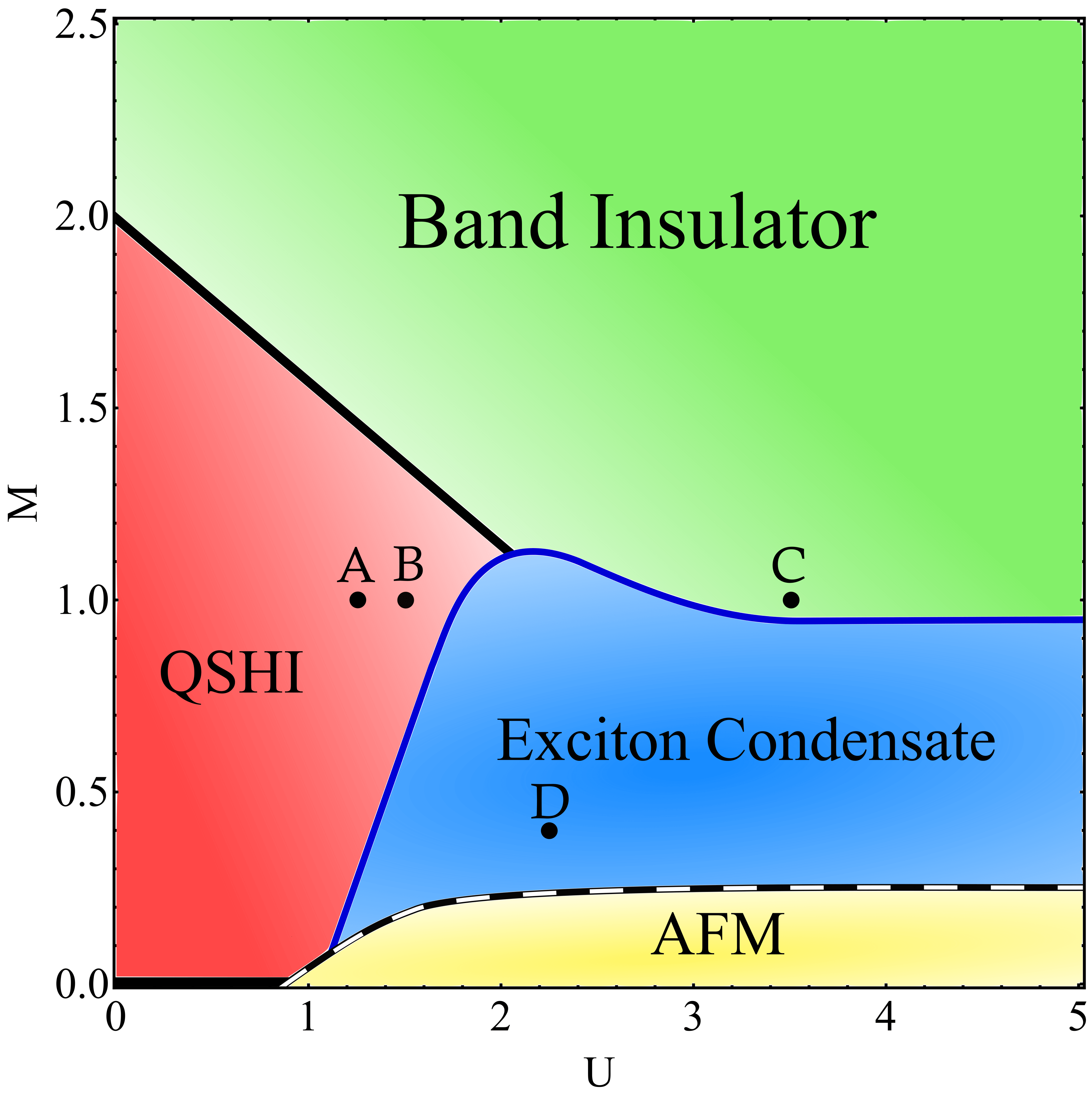
Figure 2: Hartree-Fock phase diagram at $\lambda=0.3$, $t^{\prime}=0.5$, $U_{s}=U_{p}=V=U$ and $J=U/16$. The topological insulator is denoted as QSHI, while the non topological one as Band Insulator. For small value of $M$, antiferromagnetism (AFM) is stabilised upon increasing $U$. For larger values of $M$, $U$ stabilises a symmetry broken phase with Exciton Condensate. The thick black line that separates the QSHI from the Band Insulator, as well as that at $M=0$ extending from $U=0$ to the AFM phase, indicate a gapless metallic phase. The transition between the Exciton Insulator and the QSHI or the Band Insulator is continuous, while the transition into the AFM insulator is first order.

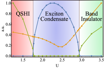
Figure 3: Order parameter $\Delta$ of Eq. (23) (blue), lowest $S_{z}=\pm 1$ exciton energy at $\mathbf{Q}={\boldsymbol{0}}$ (green), and band gap (orange) along the path A to C in Fig. 2 ($M=1$, $U\in[1.25,\,3.5]$), i.e., from the topological to the trivial insulator crossing the exciton insulator. We note that the intermediate phase emerges exactly when the exciton becomes massless, as well as that the band gap never vanishes.

As we previously mentioned, the interaction effectively increases $M$, thus pushing the transition from the topological insulator (QSHI) to the non topological one (Band Insulator) to lower values of $M$ the larger $U$. This is precisely what happens for $M\gtrsim 1.1$: $U$ increases the effective $M_{HF}$, see eq. (29), until $M_{HF}=2$. At this point the gap closes and, for still larger $U$, the QSHI turns into the trivial Band Insulator.
For very small $M\lesssim 0.2$, upon increasing $U$ the QSHI gives in to an antiferromagnetic insulator (AFM), characterised by finite order parameters $\Delta_{30}(\mathbf{R}_{i})=\Delta_{30}\,\text{e}^{i{\boldsymbol{Q}}\cdot\mathbf{R}_{i}}$, see Eq. (21), with $\mathbf{Q}=(\pi,\pi)$, thus magnetised along $z$. HF predicts such transition to be of first order, in accordance to more accurate dynamical mean field theory calculations Amaricci et al. (2018), which also explains why we do not find any precursory softening of $S_{z}=0$ exciton at $\mathbf{Q}$.

More interesting is what happens for $0.2\lesssim M\lesssim 1.1$. Here, increasing the interaction $U$ drives a transition into a phase characterised by the finite order parameter in Eq. (23), thus by a spontaneous symmetry breaking of spin $U(1)$, time reversal and inversion symmetry. The breaking of time reversal allows the system moving from the QSHI to the Band Insulator without any gap closing Hughes et al. (2011); Ezawa et al. (2013); Xue and MacDonald (2018), see Fig. 3. We note that the transition into the symmetry variant phase happens to be continuous, at least within HF. As we mentioned, consistency of our approach implies that this transition must be accompanied by the softening of the excitons whose condensation signals the birth of the symmetry breaking. These excitons are those with $S_{z}=\pm 1$, and indeed get massless on both sides of the transition, see Fig. 3.

The HF numerical results in the ribbon geometry with OBC along $x$ show that electron correlations get effectively enhanced near the boundaries, Shitade et al. (2009); Medhi et al. (2012); Amaricci et al. (2017) unsurprisingly because of the reduced coordination.Borghi et al. (2009) Indeed, the order parameter is rather large at the edges, and, moving away from them, decays exponentially towards its bulk value, as expected in an insulator. Remarkably, even when the bulk is in the QSHI stability region, a finite symmetry breaking order parameter exponentially localised at the surface layer may still develop, see Fig. 4 that refers to the point B in the phase diagram of Fig. (2). In the specific two dimensional BHZ model that we study, such phenomenon is an artefact of the Hartree-Fock approximation, since the spin $U(1)$ symmetry cannot be broken along the one dimensional edges. Nonetheless, the enhanced quantum fluctuations, while preventing a genuine symmetry breaking, should all the same substantially affect the physics at the edges.

Figure 4: Left panel: exciton condensation order parameter $\Delta(x)$ in Eq. (23) as function of the $x$-coordinate in a ribbon geometry with $N_{x}=50$ sites, calculated at point B in Fig. 2 ($M=1$, $U=1.5$). Right panel: The ribbon band structure as function of the momentum $k_{y}$. We note that, even though the condensate is exponentially localised at the edges of the system, still it has a strong effect on the single-particle edge states: a gap opens between the two branches, preventing topological spin transport.

We end the discussion of the Hartree-Fock phase diagram by comparing our results with those obtained by Xue and MacDonald Xue and MacDonald (2018). These authors, too, apply the HF approximation to study the BHZ model but in the continuum limit and in presence of a long range Coulomb interaction. They also find a path between the topological insulator and the trivial one that crosses another insulating phase characterised by spontaneous time reversal symmetry breaking, which, they argue, further breaks $\text{C}_{4}$ symmetry, thus being nematic. The HF band structure that we find in the exciton condensate phase is instead perfectly $\text{C}_{4}$ invariant, which might apparently indicate that our phase and that of Ref. Xue and MacDonald, 2018 are different. In reality, we believe the two phases are just the same phase. Indeed, while it is true that the order parameter (23) is not invariant under the $\text{C}_{4}$ symmetry of Eq. (11) that changes $\phi\to\phi-\pi/2$, such shift can be reabsorbed by a $-90^{\circ}$ spin $U(1)$ rotation. In other words, the order parameter (23) is invariant under a magnetic $\text{C}^{\prime}_{4}$ symmetry of the Hamiltonian, whose generator of $\pi/2$ rotations is $L_{3}-S_{3}$ times the rotation of $\mathbf{k}$. Due to such residual symmetry, the band structure does not show nematicity, as well as the magnetoelectric tensor we shall discuss later in section V.3.

V.2 Excitons and their topological properties

The mechanism that triggers exciton topology is similar to the band inversion in the single-particle case: a topological exciton is composed by particle-hole excitations that have different parity under inversion in different regions of the BZ. In our case study, four possible orbital channels $\tau_{a}$, $a=0,\dots,3$, are allowed, each possessing a well defined parity: $\tau_{1}$ and $\tau_{2}$ odd, while $\tau_{0}$ and $\tau_{3}$ even. In the non-topological insulator, the $S_{z}=\pm 1$ excitons have the same parity character at all inversion invariant $\mathbf{k}$-points, ${\boldsymbol{\Gamma}}$, ${\boldsymbol{M}}$, ${\boldsymbol{X}}$ and ${\boldsymbol{Y}}$, and thus are topologically trivial. On the contrary, in the QSHI, the highly mixed bands entail that all channels have finite weight in the exciton, which may acquire non trivial topology when its symmetry under parity changes among the inversion invariant $\mathbf{k}$-points, thus entailing one or more avoided crossings.

In Fig. 5 we show the Chern number of the lowest energy exciton branch with $S_{z}=-1$ calculated through Eq. (34) with $U_{s}=U_{p}=V=1.5$ as function of $M$ and $J$ along the way from the QSHI to the symmetry broken phase where excitons condense. We observe that the dipole-dipole interaction $J$ favours not only the instability of the $S_{z}=\pm 1$ excitons, but also their non trivial topology, signalled by a non zero Chern number. In Fig. 6 we show for the two points E and F in Fig. 5 the $S_{z}=-1$ exciton bands, $\omega_{i}(\mathbf{q})$, $i=1,2$ along high-symmetry paths in the BZ, together with the continuum of $S_{z}=-1$ particle-hole excitations, bounded from below by $\omega_{\text{min}}(\mathbf{q})$, see Eq. (31). The upper branch is very lightly bound, and almost touch the continuum, unlike the lower branch, whose binding energy is maximum at the ${\boldsymbol{\Gamma}}$ point where, eventually, the condensation will take place. The blue and red colours indicate, respectively, even (+) and odd (-) parity character under inversion. We note that at point F in Fig. 5 both exciton bands have vanishing Chern number, signalled by the same parity character at all inversion-invariant $\mathbf{k}$-points. On the contrary, at point E, close to the transition, the two exciton branches change parity character among the high-symmetry points, and thus acquire finite and opposite Chern numbers, $C=\pm 2$.

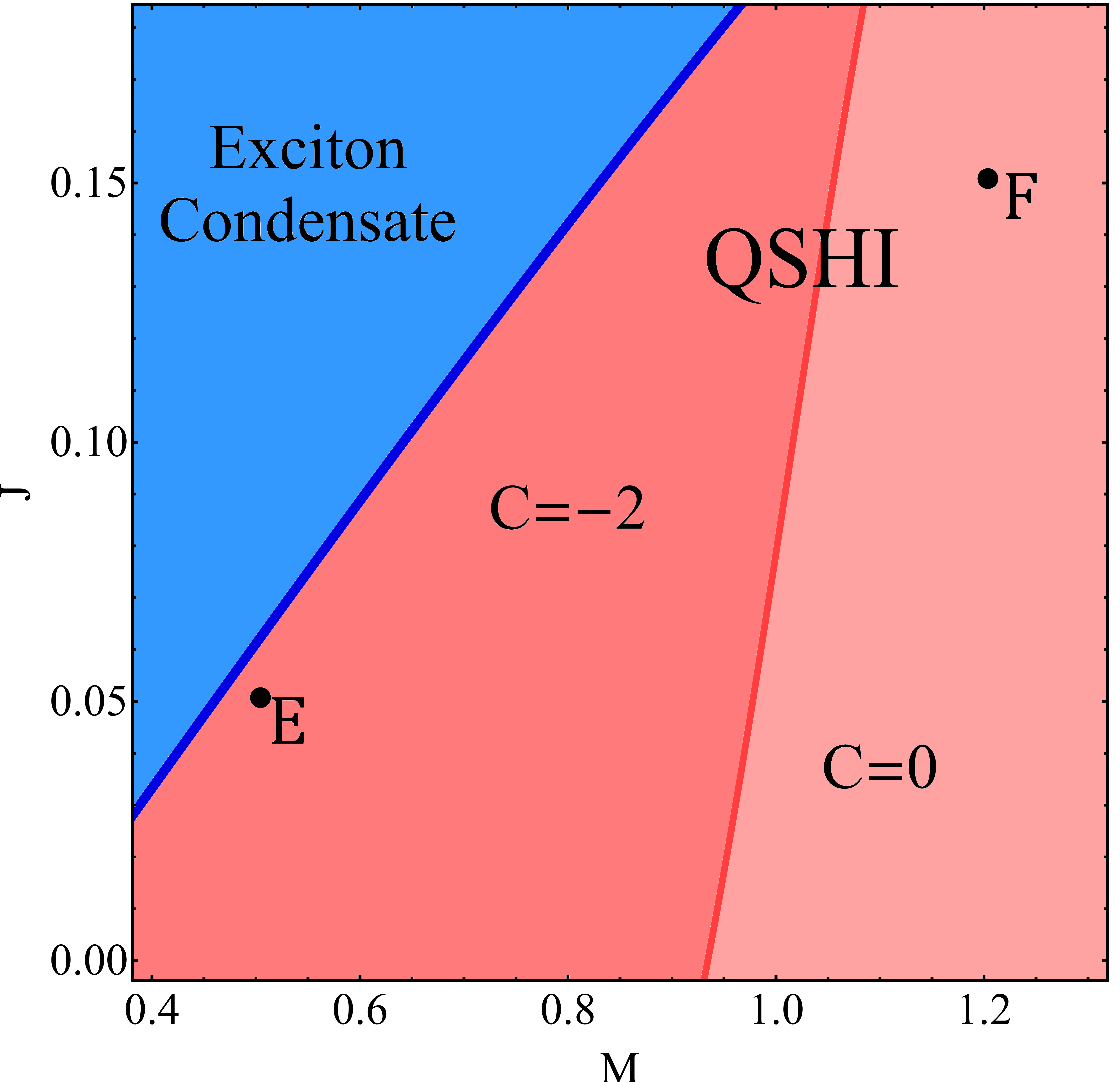
Figure 5: Chern number of the most bound exciton with $S_{z}=-1$ at $\lambda=0.3$, $t^{\prime}=0.5$, $U_{s}=U_{p}=V=1.5$, as function of $M$ and $J$ close to the transition from the QSHI to the symmetry broken phase.

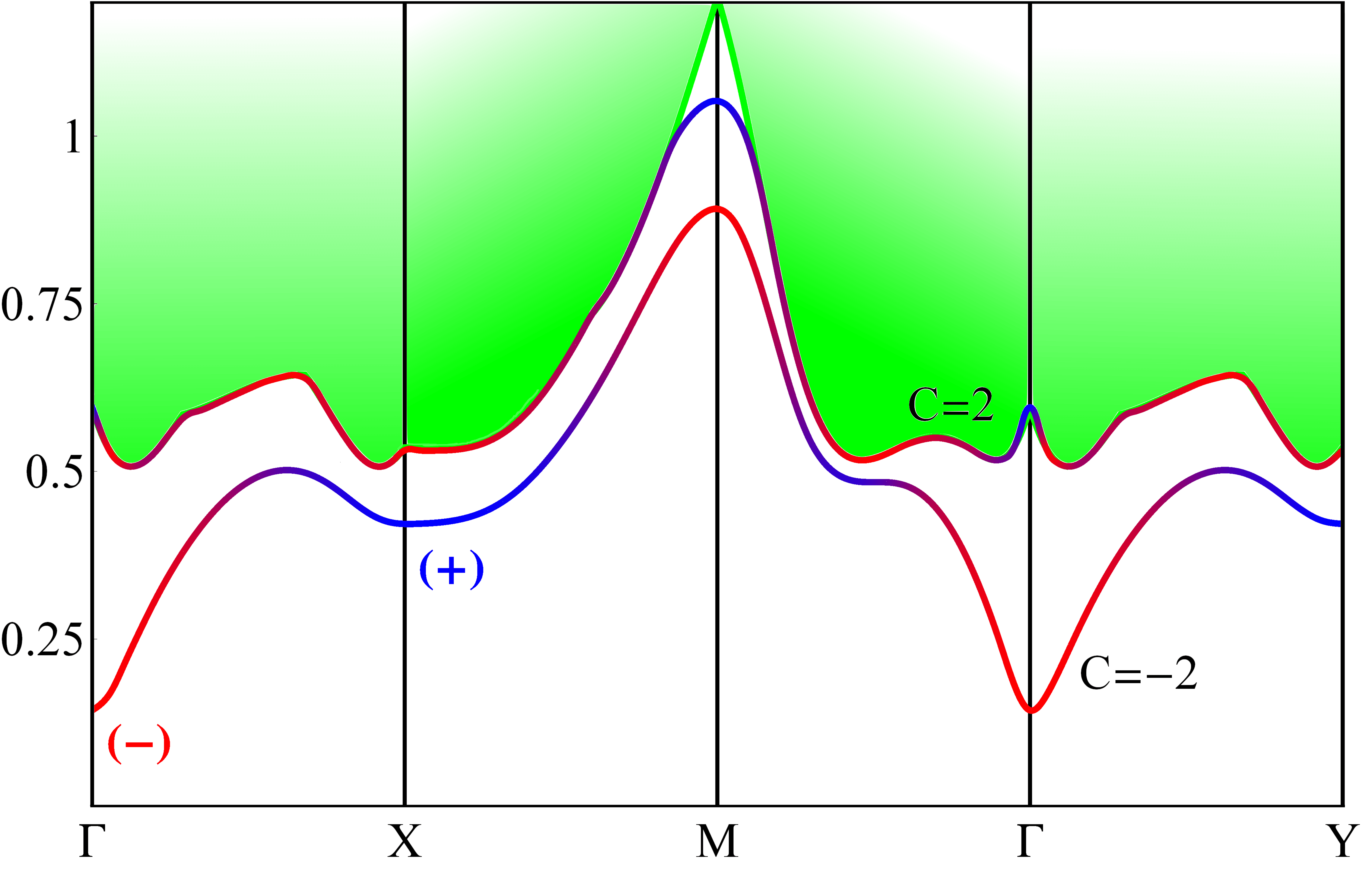
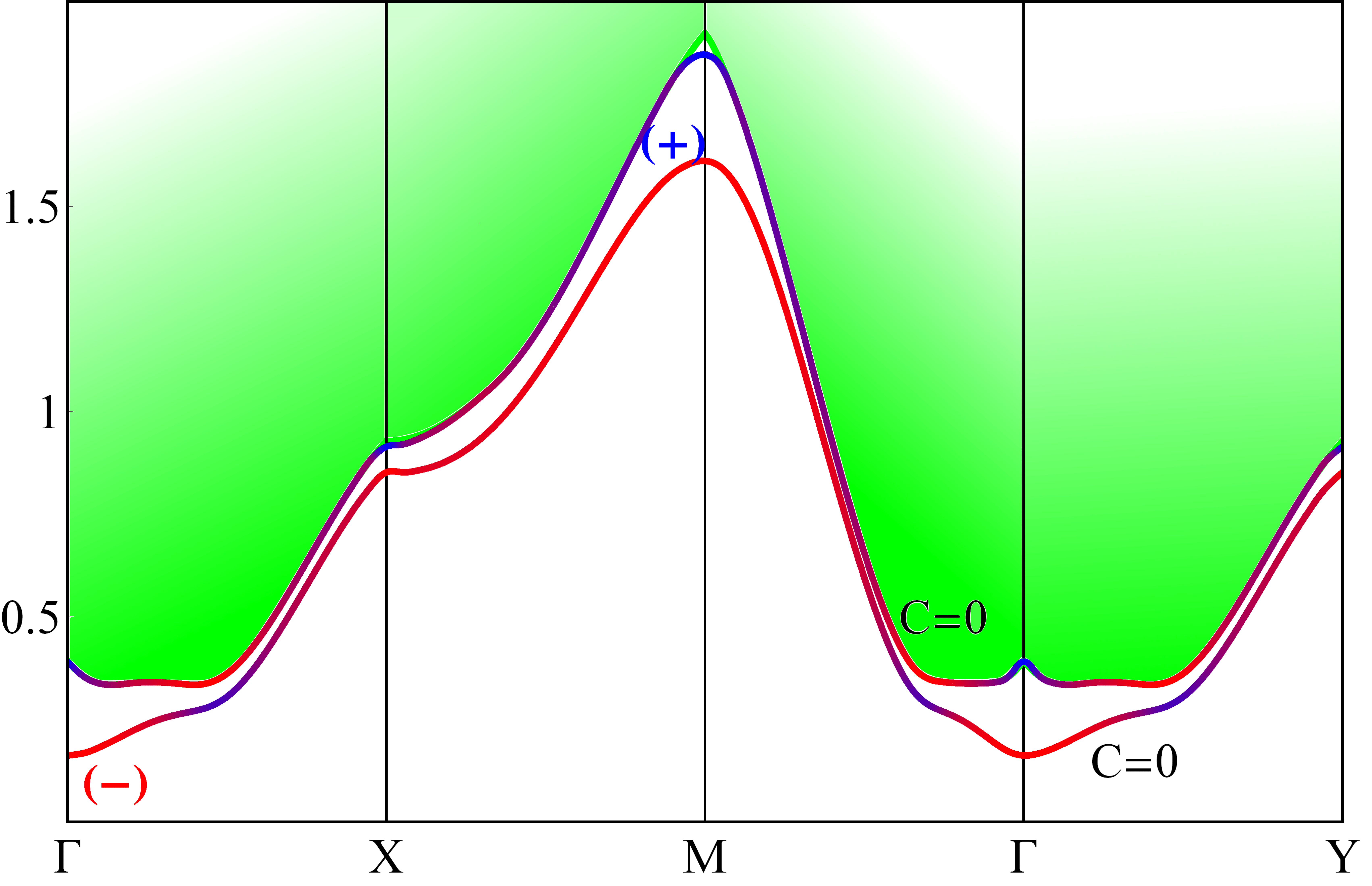
Figure 6: $S_{z}=-1$ exciton dispersion along high-symmetry paths in the Brillouin zone, calculated for the two points E, top panel, and F, bottom panel, in Fig. 5. The green shaded regions are the particle-hole continuum. The blue and red colours of the curves indicate even (+) and odd (-) parity under inversion, while $C$ is the corresponding Chern number.

For completeness, in Fig. 7 we show at the same points E and F of Fig. 5 the dispersion of the $S_{z}=0$ excitons. Since they are invariant under time reversal, we also indicate their symmetry, even (black dots) or odd (yellow dots), which correspond, respectively, to the spin singlet and spin triplet with $S_{z}=0$ components of the exciton.
Comparing Fig. 7 with 6, we note that the $S_{z}=0$ excitons are far less bound than the $S_{z}=-1$ ones. However, it is conceivable that the inclusion of the long range part of the Coulomb interaction could increase the binding energy of the $S_{z}=0$ excitons, even though we believe that the $S_{z}=\pm 1$ excitons will still be lower in energy.

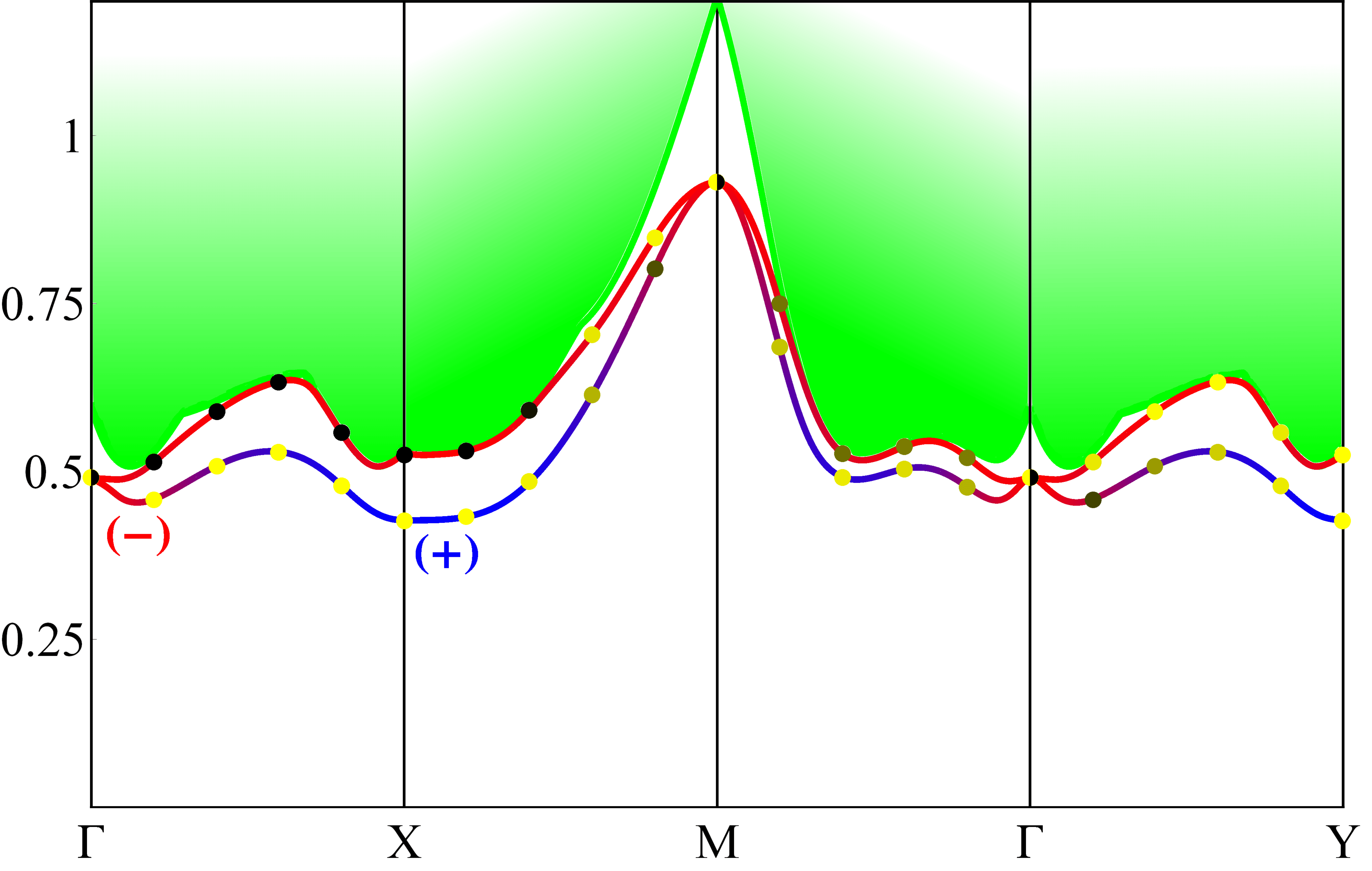
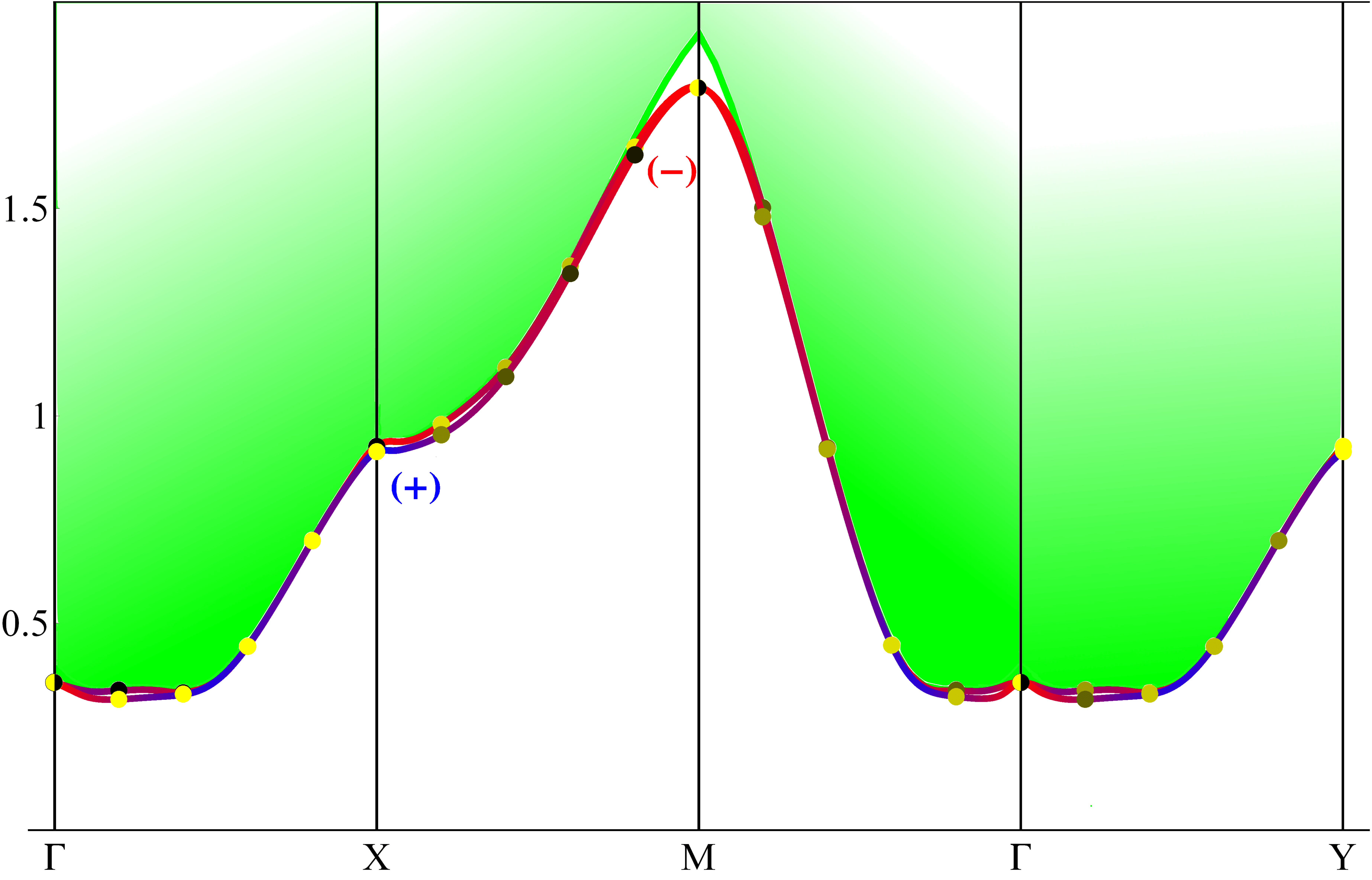
Figure 7: Same as Fig. 6 but for the $S_{z}=0$ excitons. Black and yellow dots indicate that the excitons are, respectively, even and odd under time reversal.

Moving to the sample surface at point E we expect two phenomena to occur. First, chiral exciton edge modes should appear, and connect the two branches with opposite Chern numbers, in analogy with the single particle case, and as thoroughly discussed by the authors of Ref. Chen and Shindou, 2017 in the magnetised BHZ model. In addition, our previous results in the ribbon geometry, showing that the exciton condensate appears on the surface earlier than the bulk, suggest the existence of genuine surface excitons, more bound than their bulk counterparts, definitely in the $S_{z}=\pm 1$ channel, but possibly also in the $S_{z}=0$ one.
Both the chiral exciton edge modes as well as the surface excitons may potentially have important effects on the physical behaviour at the boundaries. First of all, since the most bound ones correspond to coherent $S_{z}=\pm 1$ particle-hole excitations, they may provide efficient decay channels for the single-particle edge modes, which are counter propagating waves with opposite $S_{z}=\pm 1/2$. Experimental evidences of such phenomenon in the purported topological Kondo insulator $\text{Sm}\text{B}_{6}$ have been indeed observed Park et al. (2016); Arab et al. (2016), and previously attributed to scattering off bulk excitons Kapilevich et al. (2015). This is well possible, but should be much less efficient than the scattering off surface exciton modes, which we propose as an alternative explanation. Furthermore, the presence of odd-parity excitons localised at the surface might have direct consequences on the surface optical activity, which could be worth investigating.

V.3 Exciton condensate and magnetoelectricity

Since the order parameter in the phase with exciton condensation breaks spin $U(1)$ symmetry, inversion $\mathcal{I}$ and time reversal $\mathcal{T}$, but not $\mathcal{T}\times\mathcal{I}$, it is eligible to display magnetoelectric effects, which can be experimentally detected.
The free energy density expanded up to second order in the external electric and magnetic fields, both assumed constant in space and time, can be written as

$$F(\mathbf{E},\mathbf{B})=F_{0} -\frac{\displaystyle\;1\;}{\displaystyle\;2\;}\,{\boldsymbol{E}}\cdot\hat{\chi}_{e}\,{\boldsymbol{E}}-\frac{\displaystyle\;1\;}{\displaystyle\;2\;}\,{\boldsymbol{B}}\cdot\hat{\chi}\,{\boldsymbol{B}}$$ (35)

$$\qquad-{\boldsymbol{E}}\cdot\hat{\alpha}\,{\boldsymbol{B}}\,,$$

where $\hat{\chi}_{e}$, $\hat{\chi}$ and $\hat{\alpha}$ are the electric polarisability, magnetic susceptibility, and magnetoelectric tensors, respectively. The magnetization, ${\boldsymbol{M}}$, and polarization, ${\boldsymbol{P}}$, are conjugate variables of the fields, namely

$${\boldsymbol{M}} =-\frac{\partial F}{\partial{\boldsymbol{B}}}=\hat{\chi}\,{\boldsymbol{B}}+\hat{\alpha}\,{\boldsymbol{E}}\,,$$ (36)

$${\boldsymbol{P}} =-\frac{\partial F}{\partial{\boldsymbol{E}}}=\hat{\chi}_{e}\,{\boldsymbol{E}}+\hat{\alpha}\,{\boldsymbol{B}}\,.$$

We observe that, since ${\boldsymbol{E}}$ and ${\boldsymbol{B}}$ have opposite properties under inversion and time reversal, a non-zero $\hat{\alpha}$ is allowed only when both symmetries are broken, but not their product.
Since the exciton condensate Eq. (23) is spin-polarised in the $x\!-\!y$ plane, with azimuthal angle $\phi$, and involves dipole excitations $s\leftrightarrow p_{\pm 1}$, see Eq. (1), we restrict our analysis to fields ${\boldsymbol{E}}$ and ${\boldsymbol{B}}$ that have only $x$ and $y$ components, which allows us discarding the electromagnetic coupling to the electron charge current. Consequently, the magnetoelectric tensor $\hat{\alpha}$ of our interest will be a $2\times 2$ matrix with components $\alpha_{ij}$, $i,j=x,y$.

In the exciton condensed phase, which is insulating, the coupling to the planar electric field is via the polarisation density, namely, in proper units,

$$\delta H_{E} =-\sum_{i}\,{\boldsymbol{\Psi}}_{i}^{\dagger}\,\Big{(}\,E_{x}\,\hat{d}_{x}+E_{y}\,\hat{d}_{y}\,\Big{)}\,{\boldsymbol{\Psi}}^{\phantom{\dagger}}_{i}\,,$$ (37)

with dipole operators

$$\hat{d}_{x} =\sigma_{0}\otimes\tau_{1}\,, \hat{d}_{y} =\sigma_{3}\otimes\tau_{2}\,.$$ (38)

Moreover, as the orbitals $\ket{s\,\sigma}$ have physical total momentum $J_{z}=L_{z}+S_{z}=\pm 1/2$, while $\ket{p\,\sigma}$ have $J_{z}=\pm 3/2$, the in-plane magnetic field only couples to the magnetic moment of the $s$-orbitals. Specifically,

$$\delta H_{B} =-\sum_{i}\,{\boldsymbol{\Psi}}_{i}^{\dagger}\,\Big{(}\,B_{x}\,\hat{m}_{x}+B_{y}\,\hat{m}_{y}\,\Big{)}\,{\boldsymbol{\Psi}}^{\phantom{\dagger}}_{i}\,,$$ (39)

where

$$\hat{m}_{x} =\sigma_{1}\otimes\frac{\tau_{0}+\tau_{3}}{2}\;, \hat{m}_{y} =\sigma_{2}\otimes\frac{\tau_{0}+\tau_{3}}{2}\;.$$ (40)

Since we are interested in the effects of the external fields once the the symmetry has been broken, we performed a non self-consistent calculation with the HF self-energy calculated at ${\boldsymbol{E}}={\boldsymbol{B}}={\boldsymbol{0}}$. The finite magnetoelectric effect in the presence of the exciton condensate is indeed confirmed, see Fig. 8 where we show the components of $\hat{\alpha}$ as function of the azimuthal angle $\phi$ in Eq. (23), and which we find to behave as

$$\hat{\alpha}=\alpha_{0}\begin{pmatrix}-\cos\phi&-\sin\phi\\ -\sin\phi&\cos\phi\end{pmatrix}\,,$$ (41)

where $\alpha_{0}$ is proportional to the amplitude $\Delta$ of the order parameter, see Eq. (23), and thus vanishes when the symmetry is restored.
We remark that the magnetoelectric tensor (41) has the form predicted for the magnetic point group $4^{\prime}$ Rivera (2009), thus not showing signals of the nematic order proposed in Ref. Xue and MacDonald, 2018, as we earlier discussed in section V.1.

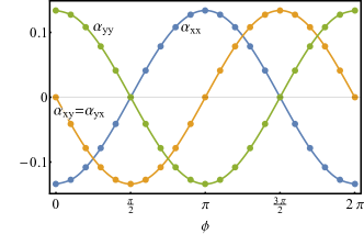
Figure 8: Components of the magnetoelectric tensor $\hat{\alpha}$ calculated at the point D in Fig. 2 ($M=0.5$, $U=2$). The data fit perfectly with the expression in Eq. (41).

VI Conclusions

In this work we have studied within a conserving mean-field scheme the role of a local electron repulsion in the prototype BHZ model of a quantum spin Hall insulator Bernevig et al. (2006), whose symmetries allows, besides the conventional monopole components of Coulomb interaction, also a dipolar one, which we find to play a rather important role.
In absence of interaction, the BHZ model displays, as function of a mass parameter $M>0$, two insulating phases, one topological at $M<M_{c}$, and another non-topological above $M_{c}$, separated by a metal point with Dirac-like dispersion at $M=M_{c}$. The primary effect of Coulomb interaction, namely the level repulsion between occupied and unoccupied states, pushes the critical $M_{c}$ to lower values, thus enlarging the stability region of the non-topological insulator. Besides that, and for intermediate values of $M$, our mean field results predict that interaction makes a new insulating phase to intrude between the topological and non-topological insulators, uncovering a path connecting the latter two that does not cross any metal point. In this phase, inversion symmetry and time reversal are spontaneously broken, though their product is not, implying the existence of magnetoelectric effects. The approach to this phase from both topological and non-topological sides is signalled by the softening of two exciton branches, related to each other by time-reversal and possessing, for $M\lesssim 1$ with the parameters of Fig. 2, finite and opposite Chern numbers. This phase can therefore be legitimately regarded as a condensate of topological excitons.
Since, starting from the quantum spin Hall insulator, the softening of those excitons and their eventual condensation occurs upon increasing the interaction, it is rather natural to expect those phenomena to be enhanced at the surface layers. Indeed, the mean field approach in a ribbon geometry predicts the surface instability to precede the bulk one. Even though a genuine exciton condensation at the surface layer might be prevented by quantum and thermal fluctuations, still it would sensibly affect the physics at the surface. The simplest consequence we may envisage is that the soft surface excitons would provide an efficient decay channel for the chiral single-particle edge modes, as indeed observed in the supposedly three-dimensional topological Kondo insulator $\text{Sm}\text{B}_{6}$ Park et al. (2016); Arab et al. (2016). In addition, we cannot exclude important consequences on the transport properties and optical activity at the surface.
We believe that going beyond the approximations assumed throughout this paper should not significantly alter our main results. RPA plus exchange allows accessing in a simple way collective excitations, though it ignores their mutual interaction. We expect that the latter would surely affect the precise location of the transition points, but not wash out the exciton condensation.
Inclusion of the neglected long range tail of Coulomb interaction would introduce two terms: the standard monopole-monopole charge repulsion, proportional to $1/r$, and a dipole-dipole interaction decaying as $1/r^{3}$. The former is expected to increase the exciton binding energy, though without distinguishing between spin singlet and triplet channels. Therefore, our conclusion that the $S_{z}=\pm 1$ excitons soften earlier than the $S_{z}=0$ ones should remain even in presence of the $1/r$ tail of Coulomb interaction. The dipole-dipole interaction might instead favour an inhomogeneous exciton condensation. However, we suspect that the $1/r^{3}$ decay in two dimensions is not sufficient to stablize domains.
To conclude, we believe that our results, though obtained by a mean field calculation and for a specific model topological insulator, catch sight of still not fully explored effects of electron electron interaction in topological insulators, which might be worth investigating experimentally, as well as theoretically in other models and, eventually, by means of more reliable tools Amaricci et al. (2015, 2016).

References

- Seradjeh et al. (2009) B. Seradjeh, J. E. Moore, and M. Franz, Phys. Rev. Lett. 103, 066402 (2009), URL https://link.aps.org/doi/10.1103/PhysRevLett.103.066402.
- Pikulin and Hyart (2014) D. I. Pikulin and T. Hyart, Phys. Rev. Lett. 112, 176403 (2014), URL https://link.aps.org/doi/10.1103/PhysRevLett.112.176403.
- Budich et al. (2014) J. C. Budich, B. Trauzettel, and P. Michetti, Phys. Rev. Lett. 112, 146405 (2014), URL https://link.aps.org/doi/10.1103/PhysRevLett.112.146405.
- Fuhrman et al. (2015) W. T. Fuhrman, J. Leiner, P. Nikolić, G. E. Granroth, M. B. Stone, M. D. Lumsden, L. DeBeer-Schmitt, P. A. Alekseev, J.-M. Mignot, S. M. Koohpayeh, et al., Phys. Rev. Lett. 114, 036401 (2015), URL https://link.aps.org/doi/10.1103/PhysRevLett.114.036401.
- Park et al. (2016) W. K. Park, L. Sun, A. Noddings, D.-J. Kim, Z. Fisk, and L. H. Greene, Proceedings of the National Academy of Sciences 113, 6599 (2016), ISSN 0027-8424, eprint https://www.pnas.org/content/113/24/6599.full.pdf, URL https://www.pnas.org/content/113/24/6599.
- Knolle and Cooper (2017) J. Knolle and N. R. Cooper, Phys. Rev. Lett. 118, 096604 (2017), URL https://link.aps.org/doi/10.1103/PhysRevLett.118.096604.
- Du et al. (2017) L. Du, X. Li, W. Lou, G. Sullivan, K. Chang, J. Kono, and R.-R. Du, Nature Communications 8, 1971 (2017), URL https://doi.org/10.1038/s41467-017-01988-1.
- Kung et al. (2019) S. Kung, A. Goyal, D. Maslov, X. Wang, A. Lee, A. Kemper, S.-W. Cheong, and G. Blumberg, Proceedings of the National Academy of Sciences 116, 201813514 (2019).
- Varsano et al. (2020) D. Varsano, M. Palummo, E. Molinari, and M. Rontani, Nature Nanotechnology 15, 367 (2020), URL https://doi.org/10.1038/s41565-020-0650-4.
- Qian et al. (2014) X. Qian, J. Liu, L. Fu, and J. Li, Science 346, 1344 (2014), ISSN 0036-8075, eprint https://science.sciencemag.org/content/346/6215/1344.full.pdf, URL https://science.sciencemag.org/content/346/6215/1344.
- Tang et al. (2017) S. Tang, C. Zhang, D. Wong, Z. Pedramrazi, H.-Z. Tsai, C. Jia, B. Moritz, M. Claassen, H. Ryu, S. Kahn, et al., Nature Physics 13, 683 (2017), URL https://doi.org/10.1038/nphys4174.
- Peng et al. (2017) L. Peng, Y. Yuan, G. Li, X. Yang, J.-J. Xian, C.-J. Yi, Y.-G. Shi, and Y.-S. Fu, Nature Communications 8, 659 (2017), URL https://doi.org/10.1038/s41467-017-00745-8.
- Efimkin et al. (2012) D. K. Efimkin, Y. E. Lozovik, and A. A. Sokolik, Phys. Rev. B 86, 115436 (2012), URL https://link.aps.org/doi/10.1103/PhysRevB.86.115436.
- Marchand and Franz (2012) D. J. J. Marchand and M. Franz, Phys. Rev. B 86, 155146 (2012), URL https://link.aps.org/doi/10.1103/PhysRevB.86.155146.
- Mink et al. (2012) M. P. Mink, H. T. C. Stoof, R. A. Duine, M. Polini, and G. Vignale, Phys. Rev. Lett. 108, 186402 (2012), URL https://link.aps.org/doi/10.1103/PhysRevLett.108.186402.
- Lozovik and Sokolik (2008) Y. E. Lozovik and A. A. Sokolik, JETP Letters 87, 55 (2008), URL https://doi.org/10.1134/S002136400801013X.
- Min et al. (2008) H. Min, R. Bistritzer, J.-J. Su, and A. H. MacDonald, Phys. Rev. B 78, 121401(R) (2008), URL https://link.aps.org/doi/10.1103/PhysRevB.78.121401.
- Liu et al. (2017) X. Liu, K. Watanabe, T. Taniguchi, B. I. Halperin, and P. Kim, Nature Physics 13, 746 (2017), URL https://doi.org/10.1038/nphys4116.
- Laurita et al. (2016) N. J. Laurita, C. M. Morris, S. M. Koohpayeh, P. F. S. Rosa, W. A. Phelan, Z. Fisk, T. M. McQueen, and N. P. Armitage, Phys. Rev. B 94, 165154 (2016), URL https://link.aps.org/doi/10.1103/PhysRevB.94.165154.
- Stankiewicz et al. (2019) J. Stankiewicz, M. Evangelisti, P. F. S. Rosa, P. Schlottmann, and Z. Fisk, Phys. Rev. B 99, 045138 (2019), URL https://link.aps.org/doi/10.1103/PhysRevB.99.045138.
- Hartstein et al. (2018) M. Hartstein, W. H. Toews, Y. T. Hsu, B. Zeng, X. Chen, M. C. Hatnean, Q. R. Zhang, S. Nakamura, A. S. Padgett, G. Rodway-Gant, et al., Nature Physics 14, 166 (2018), URL https://doi.org/10.1038/nphys4295.
- Kapilevich et al. (2015) G. A. Kapilevich, P. S. Riseborough, A. X. Gray, M. Gulacsi, T. Durakiewicz, and J. L. Smith, Phys. Rev. B 92, 085133 (2015), URL https://link.aps.org/doi/10.1103/PhysRevB.92.085133.
- Arab et al. (2016) A. Arab, A. X. Gray, S. Nemšák, D. V. Evtushinsky, C. M. Schneider, D.-J. Kim, Z. Fisk, P. F. S. Rosa, T. Durakiewicz, and P. S. Riseborough, Phys. Rev. B 94, 235125 (2016), URL https://link.aps.org/doi/10.1103/PhysRevB.94.235125.
- Akintola et al. (2018) K. Akintola, A. Pal, S. R. Dunsiger, A. C. Y. Fang, M. Potma, S. R. Saha, X. Wang, J. Paglione, and J. E. Sonier, npj Quantum Materials 3 (2018).
- Garate and Franz (2011) I. Garate and M. Franz, Phys. Rev. B 84, 045403 (2011), URL https://link.aps.org/doi/10.1103/PhysRevB.84.045403.
- Chen and Shindou (2017) K. Chen and R. Shindou, Phys. Rev. B 96, 161101(R) (2017), URL https://link.aps.org/doi/10.1103/PhysRevB.96.161101.
- Allocca et al. (2018) A. A. Allocca, D. K. Efimkin, and V. M. Galitski, Phys. Rev. B 98, 045430 (2018), URL https://link.aps.org/doi/10.1103/PhysRevB.98.045430.
- Bernevig et al. (2006) B. A. Bernevig, T. L. Hughes, and S.-C. Zhang, Science 314, 1757 (2006), ISSN 0036-8075, eprint https://science.sciencemag.org/content/314/5806/1757.full.pdf, URL https://science.sciencemag.org/content/314/5806/1757.
- Altmeyer et al. (2016) M. Altmeyer, D. Guterding, P. J. Hirschfeld, T. A. Maier, R. Valentí, and D. J. Scalapino, Phys. Rev. B 94, 214515 (2016), URL https://link.aps.org/doi/10.1103/PhysRevB.94.214515.
- Hughes et al. (2011) T. L. Hughes, E. Prodan, and B. A. Bernevig, Phys. Rev. B 83, 245132 (2011), URL https://link.aps.org/doi/10.1103/PhysRevB.83.245132.
- Ezawa et al. (2013) M. Ezawa, Y. Tanaka, and N. Nagaosa, Scientific Reports 3, 2790 (2013), URL https://doi.org/10.1038/srep02790.
- Xue and MacDonald (2018) F. Xue and A. H. MacDonald, Phys. Rev. Lett. 120, 186802 (2018), URL https://link.aps.org/doi/10.1103/PhysRevLett.120.186802.
- Shitade et al. (2009) A. Shitade, H. Katsura, J. Kuneš, X.-L. Qi, S.-C. Zhang, and N. Nagaosa, Phys. Rev. Lett. 102, 256403 (2009), URL https://link.aps.org/doi/10.1103/PhysRevLett.102.256403.
- Medhi et al. (2012) A. Medhi, V. B. Shenoy, and H. R. Krishnamurthy, Phys. Rev. B 85, 235449 (2012), URL https://link.aps.org/doi/10.1103/PhysRevB.85.235449.
- Amaricci et al. (2017) A. Amaricci, L. Privitera, F. Petocchi, M. Capone, G. Sangiovanni, and B. Trauzettel, Phys. Rev. B 95, 205120 (2017), URL https://link.aps.org/doi/10.1103/PhysRevB.95.205120.
- Rothe et al. (2010) D. G. Rothe, R. W. Reinthaler, C.-X. Liu, L. W. Molenkamp, S.-C. Zhang, and E. M. Hankiewicz, New Journal of Physics 12, 065012 (2010), URL https://iopscience.iop.org/article/10.1088/1367-2630/12/6/065012/meta.
- Kane and Mele (2005) C. L. Kane and E. J. Mele, Phys. Rev. Lett. 95, 226801 (2005), URL https://link.aps.org/doi/10.1103/PhysRevLett.95.226801.
- Mong and Shivamoggi (2011) R. S. K. Mong and V. Shivamoggi, Phys. Rev. B 83, 125109 (2011), URL https://link.aps.org/doi/10.1103/PhysRevB.83.125109.
- Amaricci et al. (2018) A. Amaricci, A. Valli, G. Sangiovanni, B. Trauzettel, and M. Capone, Phys. Rev. B 98, 045133 (2018), URL https://link.aps.org/doi/10.1103/PhysRevB.98.045133.
- Borghi et al. (2009) G. Borghi, M. Fabrizio, and E. Tosatti, Phys. Rev. Lett. 102, 066806 (2009), URL https://link.aps.org/doi/10.1103/PhysRevLett.102.066806.
- Rivera (2009) J. P. Rivera, The European Physical Journal B 71, 299 (2009), URL https://doi.org/10.1140/epjb/e2009-00336-7.
- Amaricci et al. (2015) A. Amaricci, J. C. Budich, M. Capone, B. Trauzettel, and G. Sangiovanni, Phys. Rev. Lett. 114, 185701 (2015), URL https://link.aps.org/doi/10.1103/PhysRevLett.114.185701.
- Amaricci et al. (2016) A. Amaricci, J. C. Budich, M. Capone, B. Trauzettel, and G. Sangiovanni, Phys. Rev. B 93, 235112 (2016), URL https://link.aps.org/doi/10.1103/PhysRevB.93.235112.